
Synergy of Sentinel-1 and Sentinel-2 Imagery for Crop Classification Based on DC-CNN

 and
and
Abstract
:
1. Introduction
- To properly exploit the polarimetric content of S-1 SAR data in crop classification, the outputs of the new polarimetric decomposition conceived in [50] by Mascolo et al., which is adapted for dual-polarimetric SAR data, are extracted from VH-VV S-1 observations. These, along with the VH and VV backscattering coefficients, are combined with MS features, and the best combination strategy was analyzed.
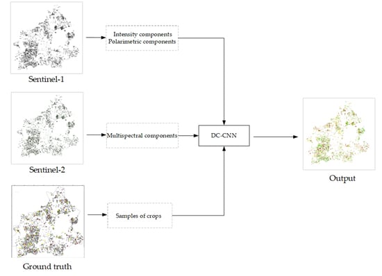
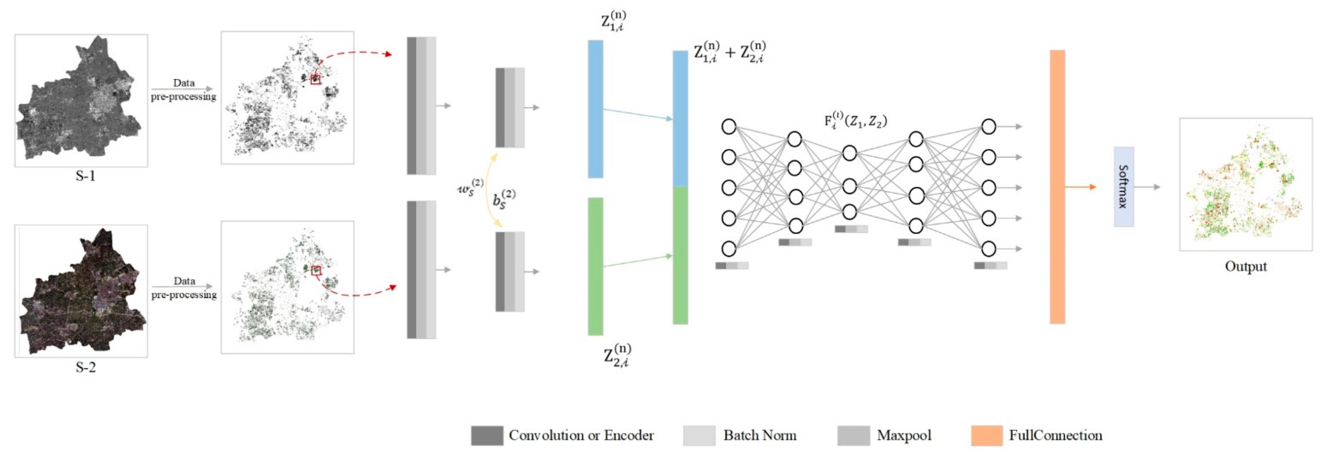
- A dual-channel CNN model, namely DC-CNN, with shared parameters based on multi-source RS data was constructed. Specifically, the features obtained from S-1 and S-2 data were fed into two CNN channels for independent learning, and they were transformed into high-dimensional feature expressions. Furthermore, the sharing of parameters in the convolution layer made the two branches learn cooperatively. The correlation of multi-source features was maximized while maintaining the unique features of each data source.
2. Materials and Methods
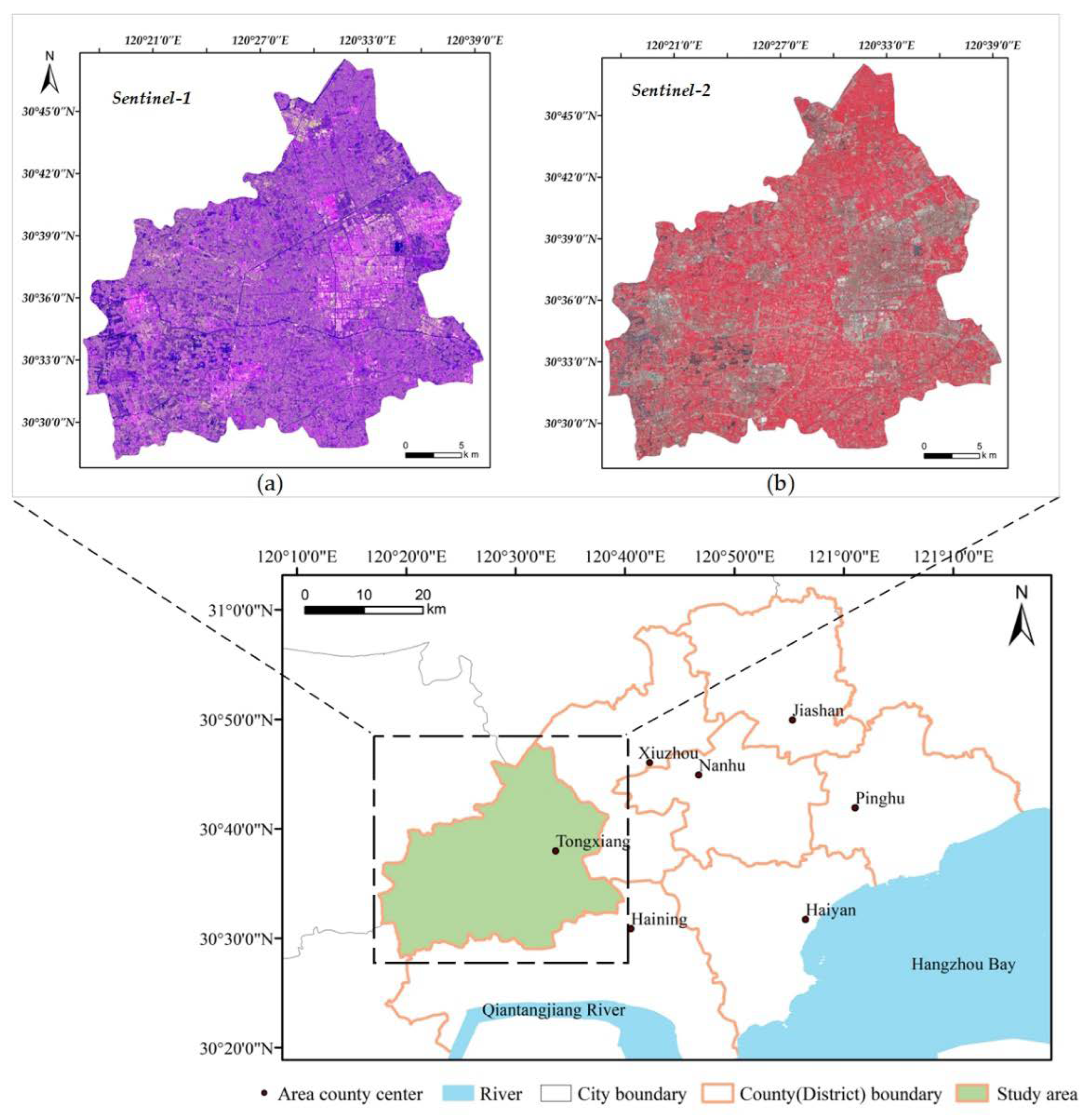
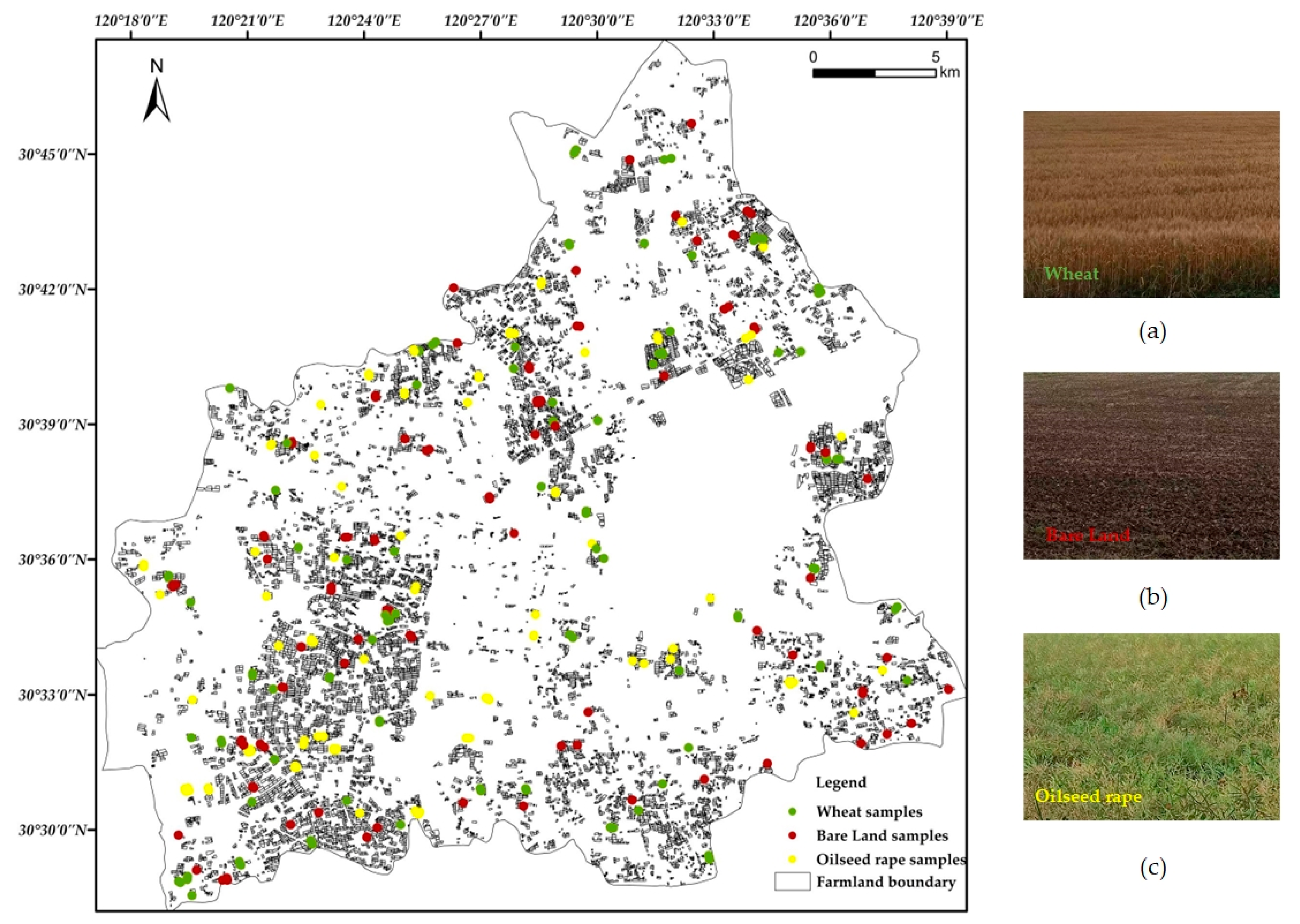
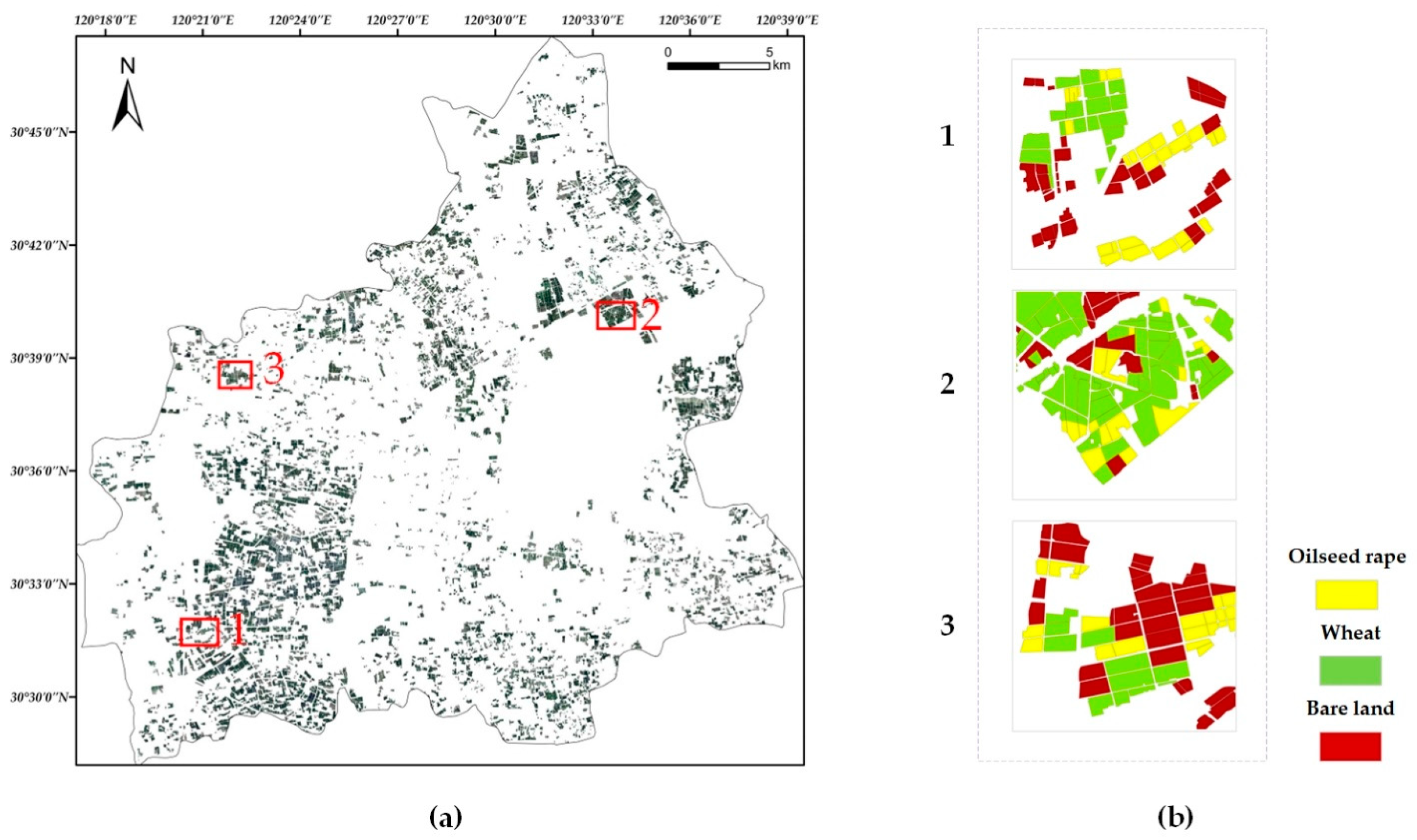
2.1. Study Area
2.2. Data and Preprocessing
2.2.1. Sentinel-1A SAR Data and Preprocessing
2.2.2. Sentinel-2B Data and Preprocessing
2.2.3. Ground-Truth Data and Preprocessing
2.3. Crop Type Classification
2.3.1. Overview
2.3.2. Polarimetric Decomposition and Feature Combination
2.3.3. Framework of DC-CNN
2.3.4. Model Accuracy Evaluation
3. Classification Results
3.1. Implementation Details
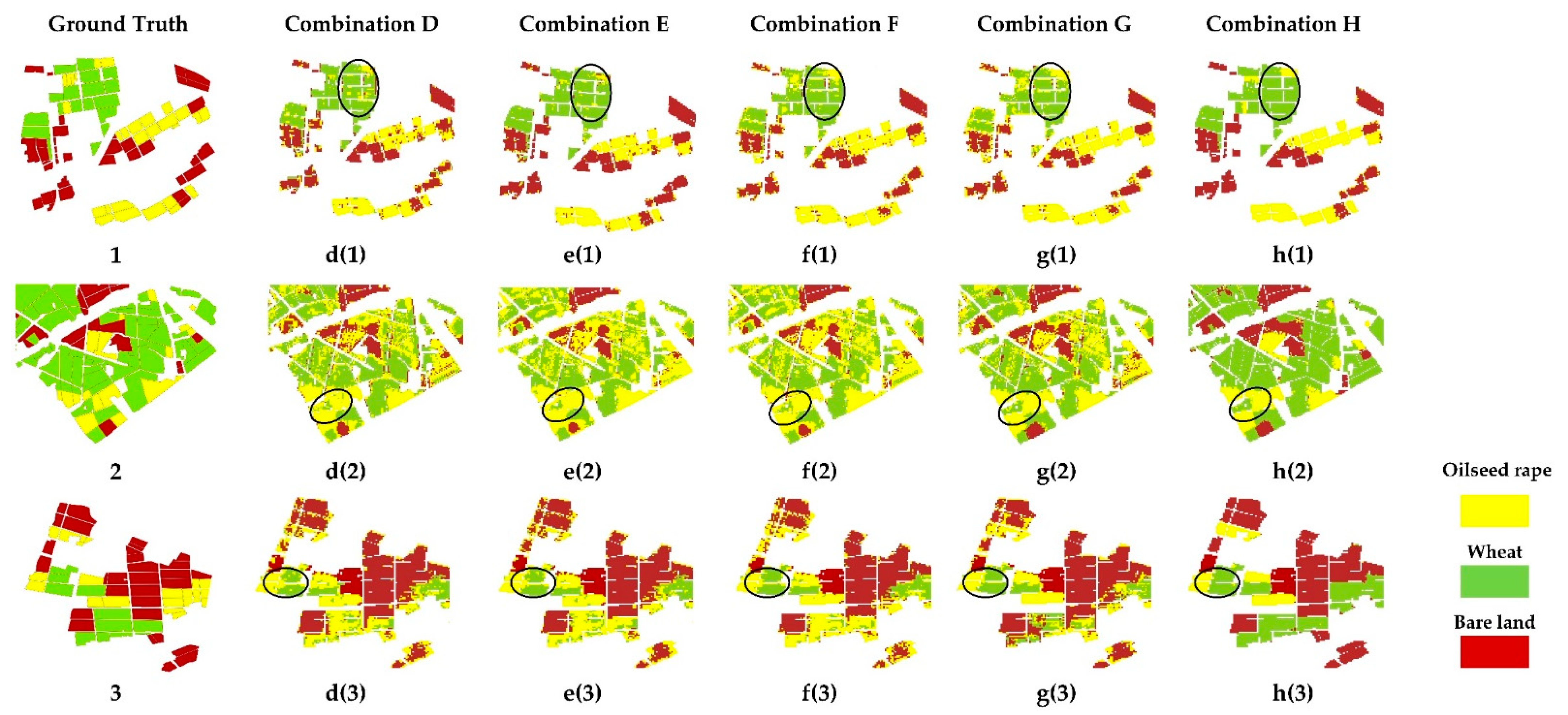
3.2. Comparison of Feature Combinations
3.2.1. Polarimetric Components in a SAR-Only Image
3.2.2. Polarimetric Components in SAR-Optical Images
3.3. Accuracy Comparison with Other Classifiers
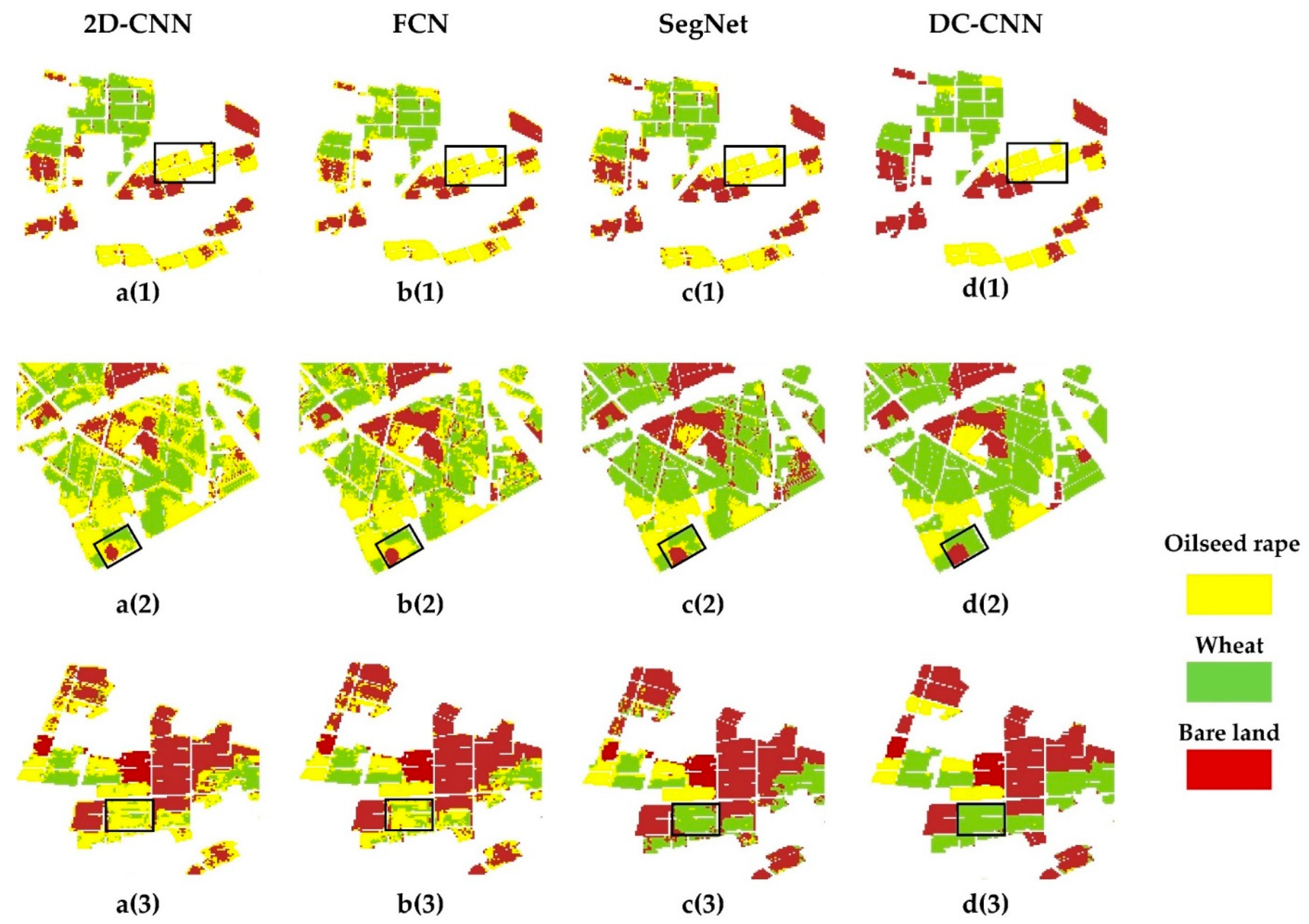
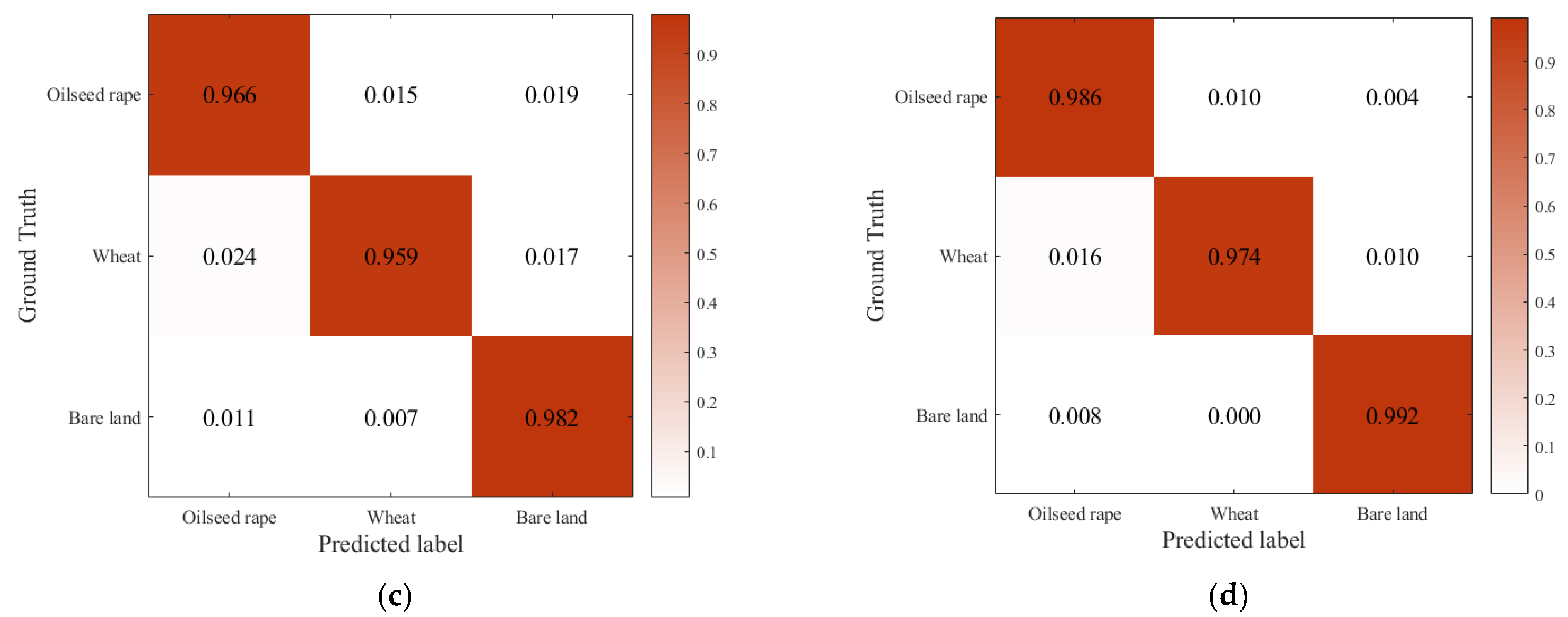
3.3.1. Qualitative Evaluation
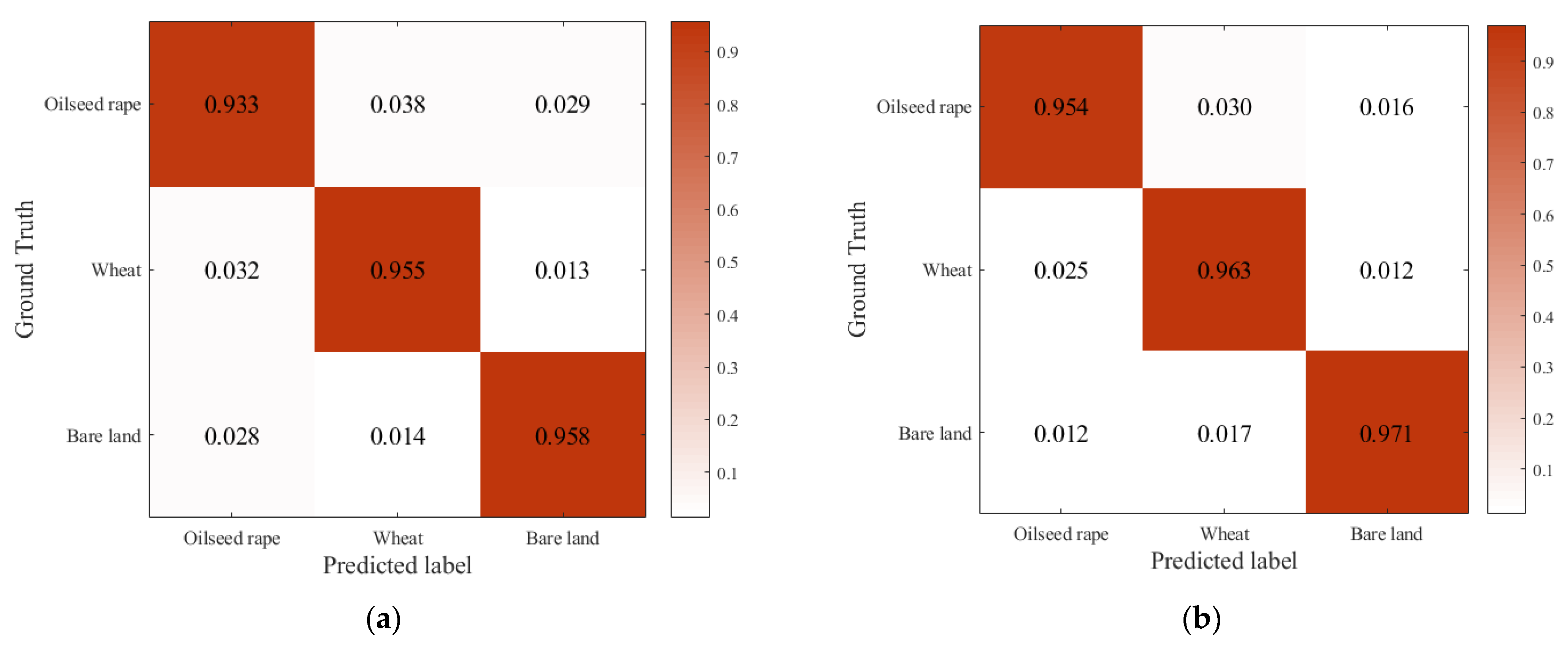
3.3.2. Quantitative Evaluation
4. Discussion
5. Conclusions
Author Contributions
Funding
Data Availability Statement
Acknowledgments
Conflicts of Interest
References
- Li, Z.; Che, G.; Zhang, T. A CNN-Transformer Hybrid Approach for Crop Classification Using Multitemporal Multisensor Images. IEEE J. Sel. Top. Appl. Earth Obs. Remote Sens. 2020, 13, 847–858. [Google Scholar] [CrossRef]
- Yang, S.; Zhang, Q.; Yuan, X.; Chen, Q.; Liu, X. Super pixel-based Classification Using Semantic Information for Polarimetric SAR Imagery. In Proceedings of the 2017 IEEE International Geoscience and Remote Sensing Symposium (IGARSS), Fort Worth, TX, USA, 23–28 July 2017; pp. 3700–3703. [Google Scholar]
- Xie, Y.; Huang, J. Integration of a Crop Growth Model and Deep Learning Methods to Improve Satellite-Based Yield620 Estimation of Winter Wheat in Henan Province, China. Remote Sens. 2021, 13, 4372. [Google Scholar] [CrossRef]
- Ezzahar, J.; Ouaadi, N.; Zribi, M.; Elfarkh, J.; Aouade, G.; Khabba, S.; Er-Raki, S.; Chehbouni, A.; Jarlan, L. Evaluation of Backscattering Models and Support Vector Machine for the Retrieval of Bare Soil Moisture from Sentinel-1 Data. Remote Sens. 2020, 12, 72. [Google Scholar] [CrossRef]
- Martos, V.; Ahmad, A.; Cartujo, P.; Ordoñez, J. Ensuring Agricultural Sustainability through Remote Sensing in the Era of Agriculture. Appl. Sci. 2021, 11, 5911. [Google Scholar] [CrossRef]
- Xie, Q.; Lai, K.; Wang, J.; Lopez-Sanchez, J.M.; Shang, J.; Liao, C.; Zhu, J.; Fu, H.; Peng, X. Crop Monitoring and Classification Using Polarimetric RADARSAT-2 Time-Series Data Across Growing Season: A Case Study in Southwestern Ontario, Canada. Remote Sens. 2021, 13, 1394. [Google Scholar] [CrossRef]
- Seifi Majdar, R.; Ghassemian, H. A Probabilistic SVM Approach for Hyperspectral Image Classification Using Spectral and Texture Features. Int. J. Remote Sens. 2017, 38, 4265–4284. [Google Scholar] [CrossRef]
- Gao, Z.; Guo, D.; Ryu, D.; Western, A.W. Enhancing the Accuracy and Temporal Transferability of Irrigated Cropping Field Classification Using Optical Remote Sensing Imagery. Remote Sens. 2022, 14, 997. [Google Scholar] [CrossRef]
- Sonobe, R.; Yamaya, Y.; Tani, H.; Wang, X.; Kobayashi, N.; Mochizuki, K.I. Mapping Crop Cover Using Multi-temporal Landsat 8 OLI Imagery. Int. J. Remote Sens. 2017, 38, 4348–4361. [Google Scholar] [CrossRef]
- Chen, J.; Liu, Y.H.; Yu, Z.R. Planting Information Extraction of Winter Wheat Based on the Time-Series MODIS-EVI. Chin. Agric. Sci. Bulletin 2011, 27, 446–450. [Google Scholar]
- Tatsumi, K.; Yamashiki, Y.; Torres, M.A.C.; Taipe, C.L.R. Crop Classification of Upland Fields using Random Forest of Time-series Landsat 7 ETM+ data. Comput. Electron. Agric. 2015, 115, 171–179. [Google Scholar] [CrossRef]
- Chabalala, Y.; Adam, E.; Ali, K.A. Machine Learning Classification of Fused Sentinel-1 and Sentinel-2 Image Data towards Mapping Fruit Plantations in Highly Heterogenous Landscapes. Remote Sens. 2022, 14, 2621. [Google Scholar] [CrossRef]
- Ma, X.; Huang, Z.; Zhu, S.; Fang, W.; Wu, Y. Rice Planting Area Identification Based on Multi-Temporal Sentinel-1 SAR Images and an Attention U-Net Model. Remote Sens. 2022, 14, 4573. [Google Scholar] [CrossRef]
- Guo, Z.; Qi, W.; Huang, Y.; Zhao, J.; Yang, H.; Koo, V.-C.; Li, N. Identification of Crop Type Based on C-AENN Using Time Series Sentinel-1A SAR Data. Remote Sens. 2022, 14, 1379. [Google Scholar] [CrossRef]
- Cable, J.W.; Kovacs, J.M.; Jiao, X.; Shang, J. Agricultural Monitoring in Northeastern Ontario, Canada, Using Multi-Temporal Polarimetric RADARSAT-2 Data. Remote Sens. 2014, 6, 2343–2371. [Google Scholar] [CrossRef]
- Xiang, H.; Luo, H.; Liu, G.; Yang, R.; Lei, X. Land Cover Classification in Mountain Areas Based on Sentinel-1A Polarimetric SAR Data and Object-Oriented Method. J. Nat. Resour. 2017, 32, 2136–3148. [Google Scholar]
- Guo, J.; Wei, P.; Zhou, Z.; Bao, S. Crop Classification Method with Differential Characteristics Based on Multi-temporal PolSAR Images. Trans. Chin. Soc. Agric. Mach. 2017, 48, 174–182. [Google Scholar]
- Xie, G.; Niculescu, S. Mapping Crop Types Using Sentinel-2 Data Machine Learning and Monitoring Crop Phenology with Sentinel-1 Backscatter Time Series in Pays de Brest, Brittany, France. Remote Sens. 2022, 14, 4437. [Google Scholar] [CrossRef]
- Orynbaikyzy, A.; Gessner, U.; Conrad, C. Crop Type Classification Using a Combination of Optical and Radar Remote Sensing Data: A Review. Int. J. Remote Sens. 2019, 40, 6553–6595. [Google Scholar] [CrossRef]
- Snevajs, H.; Charvat, K.; Onckelet, V.; Kvapil, J.; Zadrazil, F.; Kubickova, H.; Seidlova, J.; Batrlova, I. Crop Detection Using Time Series of Sentinel-2 and Sentinel-1 and Existing Land Parcel Information Systems. Remote Sens. 2022, 14, 1095. [Google Scholar] [CrossRef]
- Conrad, C.; Fritsch, S.; Zeidler, J.; Rücker, G.; Dech, S. Per-Field Irrigated Crop Classification in Arid CentralAsia Using SPOT and ASTER Data. Remote Sens. 2010, 2, 1035–1056. [Google Scholar] [CrossRef]
- Zhang, L.P.; Shen, H.F. Progress and future of remote sensing data fusion. J. Remote Sens. 2016, 20, 1050–1061. [Google Scholar]
- West, R.D.; Yocky, D.A.; Vander Laan, J.; Anderson, D.Z.; Redman, B.J. Data Fusion of Very High Resolution Hyperspectral and Polarimetric SAR Imagery for Terrain Classification. Technical Report. 2021. Available online: https://www.osti.gov/biblio/1813672 (accessed on 10 July 2021).
- Jia, K.; Li, Q.; Tian, Y.; Wu, B.; Zhang, F.; Meng, J. Crop Classification Using Multi-configuration SAR Data in the North China Plain. Int. J. Remote Sens. 2012, 33, 170–183. [Google Scholar] [CrossRef]
- Orynbaikyzy, A.; Gessner, U.; Conrad, C. Spatial Transferability of Random Forest Models for Crop Type Classification Using Sentinel-1 and Sentinel-2. Remote Sens. 2022, 14, 1493. [Google Scholar] [CrossRef]
- Mcnairn, H.; Champagne, C.; Shang, J.; Holmstrom, D.; Reichert, G. Integration of Optical and Synthetic Aperture Radar (SAR) Imagery for Delivering Operational Annual Crop Inventories. Isprs J. Photogramm. Remote Sens. 2009, 64, 434–449. [Google Scholar] [CrossRef]
- Ren, T.; Xu, H.; Cai, X.; Yu, S.; Qi, J. Smallholder Crop Type Mapping and Rotation Monitoring in Mountainous Areas with Sentinel-1/2 Imagery. Remote Sens. 2022, 14, 566. [Google Scholar] [CrossRef]
- Valero, S.; Arnaud, L.; Planells, M.; Ceschia, E. Synergy of Sentinel-1 and Sentinel-2 Imagery for Early Seasonal Agricultural Crop Mapping. Remote Sens. 2021, 13, 4891. [Google Scholar] [CrossRef]
- Veloso, A.; Mermoz, S.; Bouvet, A.; Le Toan, T.; Planells, M.; Dejoux, J.-F.; Ceschia, E. Understanding the temporal behavior of crops using Sentinel-1 and Sentinel-2-like data for agricultural applications. Remote Sens. Environ. 2017, 199, 415–426. [Google Scholar] [CrossRef]
- Zhao, H.; Chen, Z.; Jiang, H.; Jing, W.; Sun, L.; Feng, M. Evaluation of Three Deep Learning Models for Early Crop Classification Using Sentinel-1A Imagery Time Series—A Case Study in Zhanjiang, China. Remote Sens. 2019, 11, 2673. [Google Scholar] [CrossRef]
- Steinhausen, M.J.; Wagner, P.D.; Narasimhan, B.; Waske, B. Combining Sentinel-1 and Sentinel-2 data for improved land use and land over mapping of monsoon regions. Int. J. Appl. Earth Obs. Geoinf. 2018, 73, 595–604. [Google Scholar]
- Lechner, M.; Dostálová, A.; Hollaus, M.; Atzberger, C.; Immitzer, M. Combination of Sentinel-1 and Sentinel-2 Data for Tree Species Classification in a Central European Biosphere Reserve. Remote Sens. 2022, 14, 2687. [Google Scholar] [CrossRef]
- Cai, Y.T.; Lin, H.; Zhang, M. Mapping paddy rice by the object-based random forest method using time series Sentinel-1/Sentinel-2 data. Adv. Space Res. 2019, 64, 2233–2244. [Google Scholar] [CrossRef]
- Tricht, K.V.; Gobin, A.; Gilliams, S.; Piccard, I. Synergistic use of radar sentinel-1 and optical sentinel-2 imagery for crop mapping: A case study for belgium. Remote Sens. 2018, 10, 1642. [Google Scholar] [CrossRef]
- Mercier, A.; Betbeder, J.; Baudry, J.; Le Roux, L.; Spicher, F.; Lacoux, J.; Roger, D.; Hubert-Moy, L. Evaluation of Sentinel-1 & 2 time series for predicting wheat and rapeseed phenological stages. ISPRS J. Photogramm. Remote Sens. 2020, 163, 231–256. [Google Scholar]
- Sun, C.; Bian, Y.; Zhou, T.; Pan, J. Using of Multi-Source and Multi-Temporal Remote Sensing Data Improves Crop-Type Mapping in the Subtropical Agriculture Region. Sensors 2019, 19, 2401. [Google Scholar] [CrossRef] [PubMed]
- Ghassemi, B.; Immitzer, M.; Atzberger, C.; Vuolo, F. Evaluation of Accuracy Enhancement in European-Wide Crop Type Mapping by Combining Optical and Microwave Time Series. Land 2022, 11, 1397. [Google Scholar] [CrossRef]
- Zhang, L.; Duan, B.; Zou, B. Research development on target decomposition method of polarimetric SAR image. J. Electron. Inf. Technol. 2016, 38, 3289–3297. [Google Scholar]
- Cloude, S.R. Target decomposition theorems in radar scattering. Electron. Lett. 1985, 21, 22–24. [Google Scholar] [CrossRef]
- Freeman, A. Fitting a two-component scattering model to polarimetric SAR data from forests. IEEE Trans. Geosci. Remote Sens. 2007, 45, 2583–2592. [Google Scholar] [CrossRef]
- Geng, J.; Wang, H.; Fan, J.; Ma, X. SAR Image Classification via Deep Recurrent Encoding Neural Networks. IEEE Trans. Geosci. Remote Sens. 2018, 56, 2255–2269. [Google Scholar] [CrossRef]
- Wang, L.; Yang, X.; Tan, H.; Bai, X.; Zhou, F. Few-Shot Class-Incremental SAR Target Recognition Based on Hierarchical Embedding and Incremental Evolutionary Network. IEEE Trans. Geosci. Remote Sens. 2023, 61, 1–11. [Google Scholar] [CrossRef]
- Yang, Q.; Liu, M.; Zhang, Z.; Yang, S.; Ning, J.; Han, W. Mapping Plastic Mulched Farmland for High Resolution Images of Unmanned Aerial Vehicle Using Deep Semantic Segmentation. Remote Sens. 2019, 11, 2008. [Google Scholar] [CrossRef]
- Wang, H.; Chen, X.; Zhang, T.; Xu, Z.; Li, J. CCTNet: Coupled CNN and Transformer Network for Crop Segmentation of Remote Sensing Images. Remote Sens. 2022, 14, 1956. [Google Scholar] [CrossRef]
- Teimouri, N.; Dyrmann, M.; Jørgensen, R.N. A Novel Spatio-Temporal FCN-LSTM Network for Recognizing Various Crop Types Using Multi-Temporal Radar Images. Remote Sens. 2019, 11, 990. [Google Scholar] [CrossRef]
- Badrinarayanan, V.; Kendall, A.; Cipolla, R. SegNet: A Deep Convolutional Encoder-Decoder Architecture for Image Segmentation. IEEE Trans. Pattern Anal. Mach. Intell. 2017, 39, 2481–2495. [Google Scholar] [CrossRef] [PubMed]
- Kussul, N.; Lavreniuk, M.; Skakun, S.; Shelestov, A. Deep Learning Classification of Land Cover and Crop Types Using Remote Sensing Data. IEEE Geosci. Remote Sens. Lett. 2017, 14, 778–782. [Google Scholar] [CrossRef]
- Liao, C.; Wang, J.; Xie, Q.; Baz, A.A.; Huang, X.; Shang, J.; He, Y. Synergistic Use of Multi-Temporal RADARSAT-2 and VENµS Data for Crop Classification Based on 1D Convolutional Neural Network. Remote Sens. 2020, 12, 832. [Google Scholar] [CrossRef]
- Gu, L.; He, F.; Yang, S. Crop Classification based on Deep Learning in Northeast China using SAR and Optical Imagery. In Proceedings of the 2019 SAR in Big Data Era (BIGSARDATA), Beijing, China, 5–6 August 2019; pp. 1–4. [Google Scholar]
- Mascolo, L.; Cloude, S.R.; Lopez-Sanchez, J.M. Model-Based Decomposition of Dual-Pol SAR Data: Application to Sentinel-1. IEEE Trans. Geosci. Remote Sens. 2022, 60, 5220119. [Google Scholar] [CrossRef]
- Wang, H.; Yang, H.; Huang, Y.; Wu, L.; Guo, Z.; Li, N. Classification of Land Cover in Complex Terrain Using Gaofen-3 SAR Ascending and Descending Orbit Data. Remote Sens. 2023, 15, 2177. [Google Scholar] [CrossRef]
- Agilandeeswari, L.; Prabukumar, M.; Radhesyam, V.; Phaneendra, K.L.B.; Farhan, A. Crop Classification for Agricultural Applications in Hyperspectral Remote Sensing Images. Appl. Sci. 2022, 12, 1670. [Google Scholar] [CrossRef]
- Li, K.; Chen, Y. A Genetic Algorithm-Based Urban Cluster Automatic Threshold Method by Combining VIIRS DNB, NDVI, and NDBI to Monitor Urbanization. Remote Sens. 2018, 10, 277. [Google Scholar] [CrossRef]
- Mascolo, L.; Lopez-Sanchez, J.M.; Cloude, S.R. Thermal Noise Removal from Polarimetric Sentinel-1 Data. IEEE Geosci. Remote Sens. Lett. 2022, 19, 4009105. [Google Scholar] [CrossRef]
- Geng, J.; Wang, R.; Jiang, W. Polarimetric SAR Image Classification Based on Feature Enhanced Superpixel Hypergraph Neural Network. IEEE Trans. Geosci. Remote Sens. 2022, 60, 5237812. [Google Scholar] [CrossRef]
- Cloude, S.R. Polarisation: Applications in Remote Sensing; Oxford University Press: Oxford, UK, 2009. [Google Scholar]
- Lee, J.; Pottier, E. Polarimetric Radar Imaging: From Basics to Applications; CRC Press: Boca Raton, FL, USA, 2009. [Google Scholar]
- Freeman, A.; Durden, S.L. A three-component scattering model for polarimetric SAR data. IEEE Trans. Geosci. Remote Sens. 1998, 36, 963–973. [Google Scholar] [CrossRef]
- Zhou, X.; Wang, J.; He, Y.; Shan, B. Crop Classification and Representative Crop Rotation Identifying Using Statistical Features of Time-Series Sentinel-1 GRD Data. Remote Sens. 2022, 14, 5116. [Google Scholar] [CrossRef]
- Xie, Q.; Dou, Q.; Peng, X.; Wang, J.; Lopez-Sanchez, J.M.; Shang, J.; Fu, H.; Zhu, J. Crop Classification Based on the Physically Constrained General Model-Based Decomposition Using Multi-Temporal RADARSAT-2 Data. Remote Sens. 2022, 14, 2668. [Google Scholar] [CrossRef]
- Yamaguchi, Y.; Moriyama, T.; Ishido, M.; Yamada, H. Four-component scattering model for polarimetric SAR image decomposition. IEEE Trans. Geosci. Remote Sens. 2005, 43, 1699–1706. [Google Scholar] [CrossRef]
- Van Zyl, J.J.; Arii, M.; Kim, Y. Model-based decomposition of polarimetric SAR covariance matrices constrained for nonnegative eigenvalues. IEEE Trans. Geosci. Remote Sens. 2011, 9, 3452–3459. [Google Scholar] [CrossRef]
- Wang, D.; Cao, W.; Zhang, F.; Li, Z.; Xu, S.; Wu, X. A Review of Deep Learning in Multiscale Agricultural Sensing. Remote Sens. 2022, 14, 559. [Google Scholar] [CrossRef]
- Cherif, E.; Hell, M.; Brandmeier, M. DeepForest: Novel Deep Learning Models for Land Use and Land Cover Classification Using Multi-Temporal and -Modal Sentinel Data of the Amazon Basin. Remote Sens. 2022, 14, 5000. [Google Scholar] [CrossRef]
- Konapala, G.; Kumar, S.; Ahmad, S. Exploring Sentinel-1 and Sentinel-2 diversity for flood inundation mapping using deep learning. ISPRS J. Photogramm. Remote Sens. 2021, 180, 163–173. [Google Scholar] [CrossRef]
- Hartmann, A.; Davari, A.; Seehaus, T.; Braun, M.; Maier, A.; Christlein, V. Bayesian U-Net for Segmenting Glaciers in SAR Imagery. In Proceedings of the IEEE International Geoscience and Remote Sensing Symposium IGARSS, Brussels, Belgium, 11–16 July 2021; pp. 3479–3482. [Google Scholar]
- Seydi, S.T.; Amani, M.; Ghorbanian, A. A Dual Attention Convolutional Neural Network for Crop Classification Using Time-Series Sentinel-2 Imagery. Remote Sens. 2022, 14, 498. [Google Scholar] [CrossRef]
- Denize, J.; Hubert-Moy, L.; Betbeder, J.; Corgne, S.; Baudry, J.; Pottier, E. Evaluation of using sentinel-1 and -2 time-series to identify winter land use in agricultural landscapes. Remote Sens. 2019, 11, 37. [Google Scholar] [CrossRef]
- Demarez, V.; Helen, F.; Marais-Sicre, C.; Baup, F. In-season mapping of irrigated crops using Landsat 8 and Sentinel-1 time series. Remote Sens. 2019, 11, 118. [Google Scholar] [CrossRef]
- Liu, J.; Zhu, W.; Atzberger, C.; Zhao, A.; Pan, Y.; Huang, X. A phenology-based method to map cropping patterns under a wheat-maize rotation using remotely sensed time-series data. Remote Sens. 2018, 10, 1203. [Google Scholar] [CrossRef]
- Ghassemi, B.; Dujakovic, A.; Zółtak, M.; Immitzer, M.; Atzberger, C.; Vuolo, F. Designing a EuropeanWide Crop Type Mapping Approach Based on Machine Learning Algorithms Using LUCAS Field Survey and Sentinel-2 Data. Remote Sens. 2022, 14, 541. [Google Scholar] [CrossRef]
- Venter, Z.S.; Sydenham, M.A.K. Continental-Scale Land Cover Mapping at 10 m Resolution Over Europe (ELC10). Remote Sens. 2021, 13, 2301. [Google Scholar] [CrossRef]
- Qiao, C.; Daneshfar, B.; Davidson, A.; Jarvis, I.; Liu, T.; Fisette, T. (Eds.) Integration of Optical and Polarimetric SAR Imagery for Locally Accurate Crop Classification. In Proceedings of the Geoscience and Remote Sensing Symposium (IGARSS), 2014 IEEE International, Quebec City, QC, Canada, 13–18 July 2014; pp. 13–18. [Google Scholar]
- Villa, P.; Stroppiana, D.; Fontanelli, G.; Azar, R.; Brivio, A.P. In-Season Mapping of Crop Type with Optical and X-Band SAR Data: A Classification Tree Approach Using Synoptic Seasonal Features. Remote Sens. 2015, 7, 12859–12886. [Google Scholar] [CrossRef]
- Salehi, B.; Daneshfar, B.; Davidson, A.M. Accurate Crop-Type Classification Using Multi-Temporal Optical and Multi-Polarization SAR Data in an Object-Based Image Analysis Framework. Int. J. Remote Sens. 2017, 38, 4130–4155. [Google Scholar] [CrossRef]


| S-1A Parameters | S-1A |
|---|---|
| Product type | SLC |
| Imaging mode | IW |
| Polarization | VV VH |
| Pixel size | 10 m 10 m |
| Pass direction | Ascending |
| Wave band | C |
| Dates | 2021-05-06 |
| S-2 Satellite | Date | Cloud Cover Percentage (%) | S-2 Satellite | Date | Cloud Cover Percentage (%) |
|---|---|---|---|---|---|
| A | 8 April 2021 | 99.94 | B | 3 April 2021 | 99.89 |
| A | 8 April 2021 | 71.47 | B | 3 April 2021 | 99.97 |
| A | 18 April 2021 | 87.58 | B | 13 April 2021 | 53.41 |
| A | 18 April 2021 | 56.11 | B | 13 April 2021 | 88.98 |
| A | 28 April 2021 | 98.98 | B | 23 April 2021 | 98.98 |
| A | 28 April 2021 | 94.74 | B | 23 April 2021 | 98.46 |
| A | 8 May 2021 | 99.99 | B | 3 May 2021 | 11.42 |
| A | 8 May 2021 | 99.89 | B | 3 May 2021 | 19.96 |
| A | 18 May 2021 | 99.77 | B | 13 May 2021 | 99.33 |
| A | 18 May 2021 | 99.57 | B | 13 May 2021 | 98.58 |
| A | 28 May 2021 | 100 | B | 23 May 2021 | 67.47 |
| A | 28 May 2021 | 94.12 | B | 23 May 2021 | 88.47 |
| A | 7 June 2021 | 93.43 | B | 2 June 2021 | 97.03 |
| A | 7 June 2021 | 96.48 | B | 2 June 2021 | 99.29 |
| A | 17 June 2021 | 93.91 | B | 12 June 2021 | 83.16 |
| A | 17 June 2021 | 99.64 | B | 12 June 2021 | 90.27 |
| A | 27 June 2021 | 97.58 | B | 22 June 2021 | 82.89 |
| A | 27 June 2021 | 94.57 | B | 22 June 2021 | 9.47 |
| S-2B Parameters | Spatial Resolution (m) | S-2B Spectral Description |
|---|---|---|
| Band 2 | 10 | Blue |
| Band 3 | 10 | Green |
| Band 4 | 10 | Red |
| Band 5 | 20 | Vegetation red edge |
| Band 6 | 20 | Vegetation red edge |
| Band 7 | 20 | Vegetation red edge |
| Band 8 | 10 | Near Infrared |
| Band 8A | 20 | Vegetation red edge |
| Band 11 | 20 | Short-Wave Infrared |
| Band 12 | 20 | Short-Wave Infrared |
| Dates | 2021-05-03 | |
| Processing Level | Level 2A |
| Label | Type | Number of Fields | Total Number of Pixels | Number of Training Samples | Number of Validation Samples | Number of Testing Samples |
|---|---|---|---|---|---|---|
| 1 | Oilseed rape | 101 | 6038 | 3601 | 1207 | 1230 |
| 2 | Wheat | 103 | 7418 | 4458 | 1483 | 1477 |
| 3 | Bare land | 101 | 6084 | 3654 | 1216 | 1214 |
| Total | - | 305 | 19,540 | 11,713 | 3906 | 3921 |
| Combination | Abbreviation | Comment |
|---|---|---|
| A | S-1 (VV, VH) | Only the intensity components VV and VH of S1 |
| B | S-1 (, ) | Only the polarimetric components and of S1 |
| C | S-1 (VV, VH, , ) | The intensity components VV, VH, and the polarimetric components , , of S1 |
| D | S-1 (VV, VH) + S-2(MS) | The intensity components VV, VH of S1 + MS of S-2 |
| E | S-1 (, ) + S-2(MS) | The polarimetric components , of S1 + MS of S-2 |
| F | S-1 (VV, VH, ) + S-2(MS) | The intensity components VV, VH, and the polarimetric components of S1 + MS of S-2 |
| G | S-1 (VV, VH, ) + S-2(MS) | The intensity components VV, VH, and the polarimetric components of S1 + MS of S-2 |
| H | S-1 (VV, VH, , ) + S-2(MS) | The intensity components VV, VH, and the polarimetric components , of S1 + MS of S-2 |
| S-1 | S-2 | ||
|---|---|---|---|
| Conv: 3 3 16 | (n, 7, 7, 16) | Conv: 3 3 16 | (n, 7, 7, 16) |
| BN | (n, 7, 7, 16) | BN | (n, 7, 7, 16) |
| ReLU | (n, 7, 7, 16) | ReLU | (n, 7, 7, 16) |
| Max-Pooling: 2 2 | (n, 4, 4, 16) | Max-Pooling: 2 2 | (n, 4, 4, 16) |
| Conv: 3 3 32 | (n, 4, 4, 32) | Conv: 3 3 32 | (n, 4, 4, 32) |
| BN | (n, 4, 4, 32) | BN | (n, 4, 4, 32) |
| ReLU | (n, 4, 4, 32) | ReLU | (n, 4, 4, 32) |
| Max-Pooling: 2 2 | (n,2, 2, 32) | Max-Pooling: 2 2 | (n,2, 2, 32) |
| Flatten | 128 | Flatten | 128 |
| Layer | Parameters | Output shape | |
| Joint Layer | (n, 256) | ||
| Encoder1 | 128, activation = ‘ReLU ‘ | (n, 128) | |
| Encoder2 | 64, activation = ‘ReLU ‘ | (n, 64) | |
| Encoder3 | 32, activation = ‘ReLU ‘ | (n, 32) | |
| Compressed features | 16, activation = ‘ReLU ‘ | (n, 16) | |
| Decoder1 | 32, activation = ‘ReLU ‘ | (n, 32) | |
| Decoder2 | 64, activation = ‘ReLU ‘ | (n, 64) | |
| Decoder3 | 128, activation = ‘ReLU ‘ | (n, 128) | |
| Classification | SoftMax | (n, 3) | |
| Configuration | Version |
|---|---|
| GPU | GeForce RTX 3080Ti |
| Memory | 64G |
| Language | Python 3.8.3 |
| Frame | Tensorflow 1.14.0 |
| Oilseed Rape | Wheat | Bare Land | Macro-F1 | OA | Kappa | ||
|---|---|---|---|---|---|---|---|
| Combination A | Precision | 0.783 | 0.694 | 0.806 | 0.7603 | 0.7609 | 0.462 |
| Recall | 0.715 | 0.771 | 0.802 | ||||
| F1-score | 0.747 | 0.730 | 0.804 | ||||
| Combination B | Precision | 0.832 | 0.752 | 0.835 | 0.806 | 0.8061 | 0.572 |
| Recall | 0.765 | 0.825 | 0.834 | ||||
| F1-score | 0.797 | 0.787 | 0.834 | ||||
| Combination C | Precision | 0.855 | 0.780 | 0.843 | 0.828 | 0.8312 | 0.628 |
| Recall | 0.792 | 0.854 | 0.852 | ||||
| F1-score | 0.822 | 0.815 | 0.847 |
| Oilseed Rape | Wheat | Bare Land | Macro-F1 | OA | Kappa | ||
|---|---|---|---|---|---|---|---|
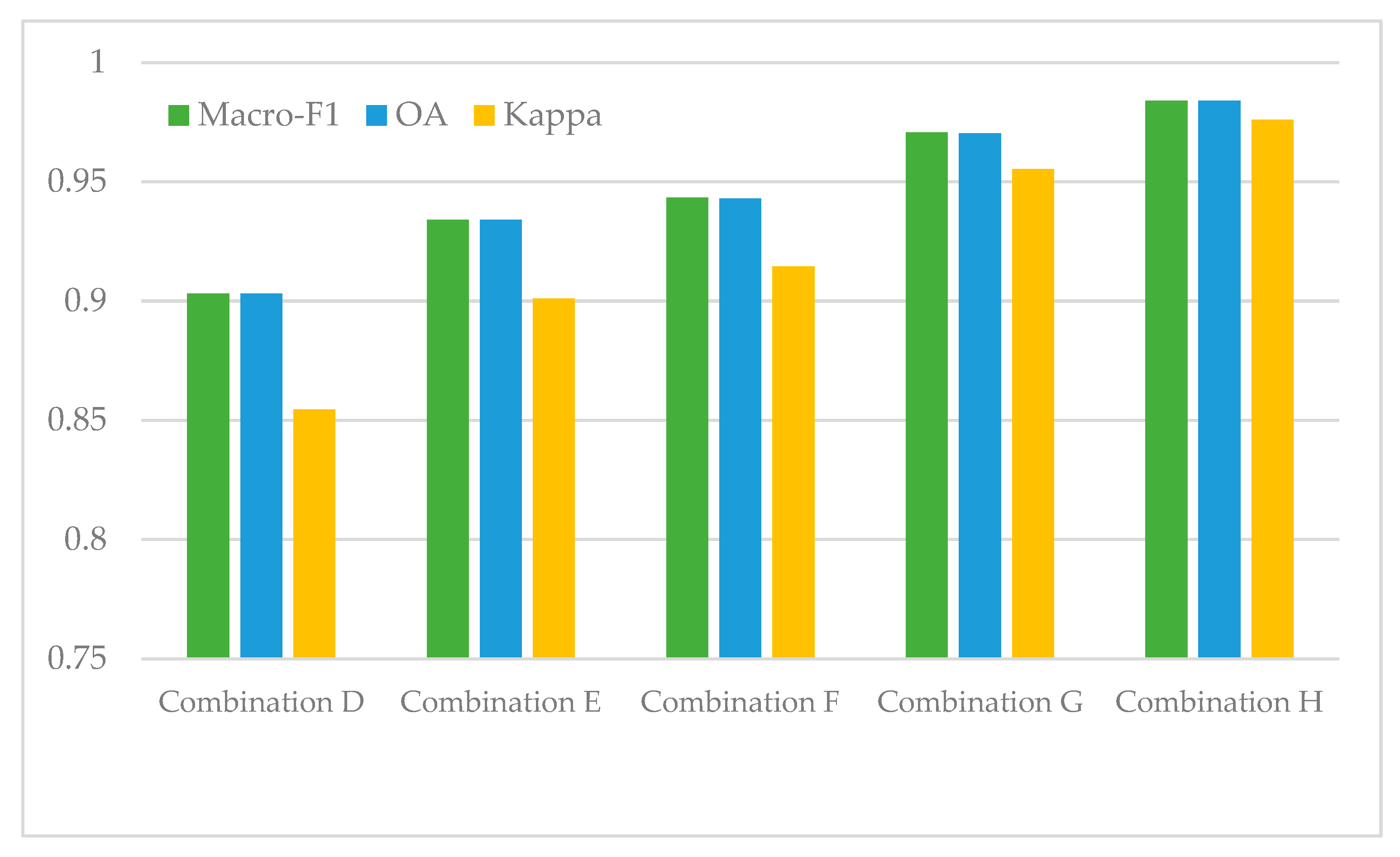
| Combination D | Precision | 0.909 | 0.889 | 0.911 | 0.9030 | 0.9030 | 0.8545 |
| Recall | 0.867 | 0.905 | 0.937 | ||||
| F1-score | 0.888 | 0.897 | 0.924 | ||||
| Combination E | Precision | 0.918 | 0.941 | 0.943 | 0.9340 | 0.9340 | 0.9010 |
| Recall | 0.919 | 0.937 | 0.946 | ||||
| F1-score | 0.919 | 0.939 | 0.945 | ||||
| Combination F | Precision | 0.940 | 0.933 | 0.956 | 0.9433 | 0.9430 | 0.9145 |
| Recall | 0.928 | 0.946 | 0.955 | ||||
| F1-score | 0.934 | 0.940 | 0.956 | ||||
| Combination G | Precision | 0.967 | 0.972 | 0.972 | 0.9707 | 0.9703 | 0.9554 |
| Recall | 0.961 | 0.967 | 0.983 | ||||
| F1-score | 0.964 | 0.970 | 0.978 | ||||
| Combination H | Precision | 0.976 | 0.990 | 0.986 | 0.9840 | 0.9840 | 0.9760 |
| Recall | 0.986 | 0.974 | 0.992 | ||||
| F1-score | 0.981 | 0.982 | 0.989 |
| Oilseed Rape | Wheat | Bare Land | Macro-F1 | OA | Kappa | ||
|---|---|---|---|---|---|---|---|
| 2D-CNN | Precision | 0.940 | 0.934 | 0.958 | 0.9467 | 0.9487 | 0.9230 |
| Recall | 0.933 | 0.955 | 0.958 | ||||
| F1-score | 0.937 | 0.945 | 0.958 | ||||
| FCN | Precision | 0.963 | 0.953 | 0.972 | 0.9630 | 0.9627 | 0.9440 |
| Recall | 0.954 | 0.963 | 0.971 | ||||
| F1-score | 0.959 | 0.958 | 0.972 | ||||
| SegNet | Precision | 0.965 | 0.978 | 0.964 | 0.9693 | 0.9690 | 0.9534 |
| Recall | 0.966 | 0.959 | 0.982 | ||||
| F1-score | 0.966 | 0.969 | 0.973 | ||||
| DC-CNN | Precision | 0.976 | 0.990 | 0.986 | 0.9840 | 0.9840 | 0.9760 |
| Recall | 0.986 | 0.974 | 0.992 | ||||
| F1-score | 0.981 | 0.982 | 0.989 |
| Macro-F1 | OA | Kappa | |
|---|---|---|---|
| S-1 (VV, VH, , ) | 0.8280 | 0.8312 | 0.6280 |
| S-2(MS) | 0.9430 | 0.8854 | 0.7403 |
| S-1 (VV, VH, , ) + S-2(MS) | 0.9840 | 0.9840 | 0.9760 |
Disclaimer/Publisher’s Note: The statements, opinions and data contained in all publications are solely those of the individual author(s) and contributor(s) and not of MDPI and/or the editor(s). MDPI and/or the editor(s) disclaim responsibility for any injury to people or property resulting from any ideas, methods, instructions or products referred to in the content. |
© 2023 by the authors. Licensee MDPI, Basel, Switzerland. This article is an open access article distributed under the terms and conditions of the Creative Commons Attribution (CC BY) license (https://creativecommons.org/licenses/by/4.0/).
Share and Cite
Zhang, K.; Yuan, D.; Yang, H.; Zhao, J.; Li, N. Synergy of Sentinel-1 and Sentinel-2 Imagery for Crop Classification Based on DC-CNN. Remote Sens. 2023, 15, 2727. https://doi.org/10.3390/rs15112727
Zhang K, Yuan D, Yang H, Zhao J, Li N. Synergy of Sentinel-1 and Sentinel-2 Imagery for Crop Classification Based on DC-CNN. Remote Sensing. 2023; 15(11):2727. https://doi.org/10.3390/rs15112727
Chicago/Turabian StyleZhang, Kaixin, Da Yuan, Huijin Yang, Jianhui Zhao, and Ning Li. 2023. "Synergy of Sentinel-1 and Sentinel-2 Imagery for Crop Classification Based on DC-CNN" Remote Sensing 15, no. 11: 2727. https://doi.org/10.3390/rs15112727