
Inversion of Soil Moisture on Farmland Areas Based on SSA-CNN Using Multi-Source Remote Sensing Data


Abstract
:
1. Introduction
2. Materials and Methods
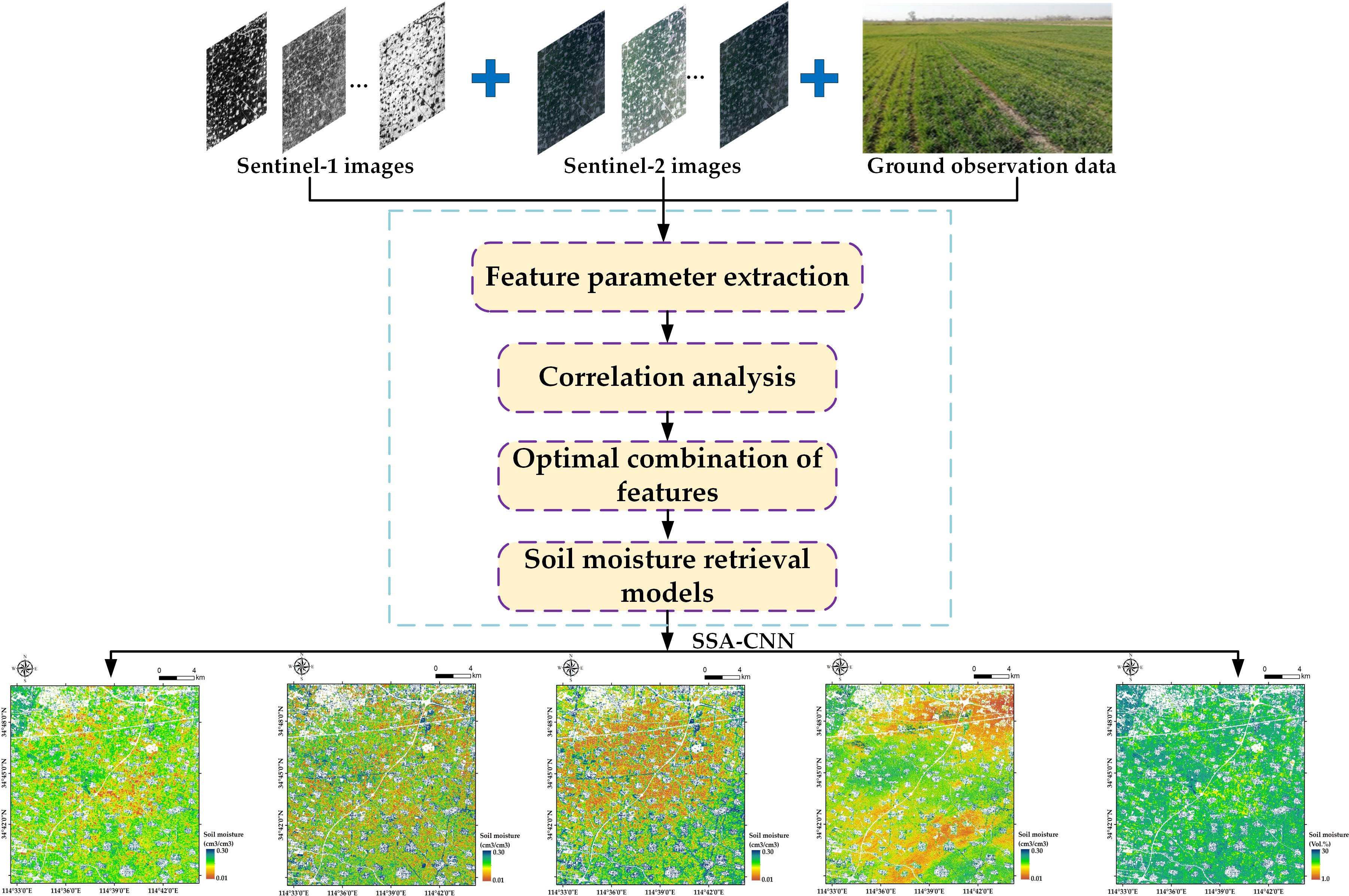
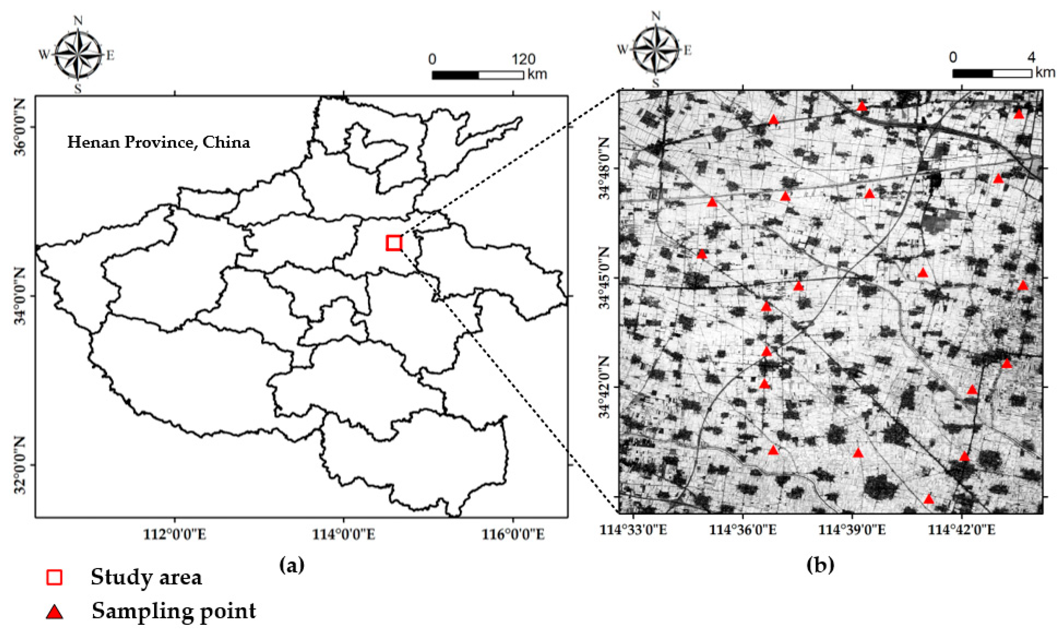
2.1. Study Area
2.2. Data Set and Image Preprocessing
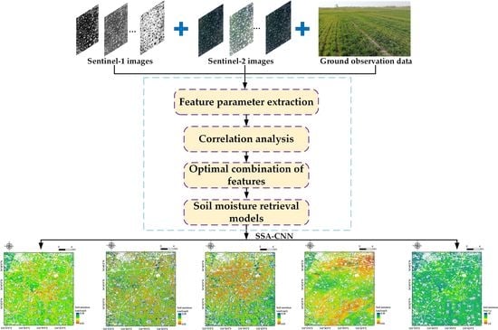
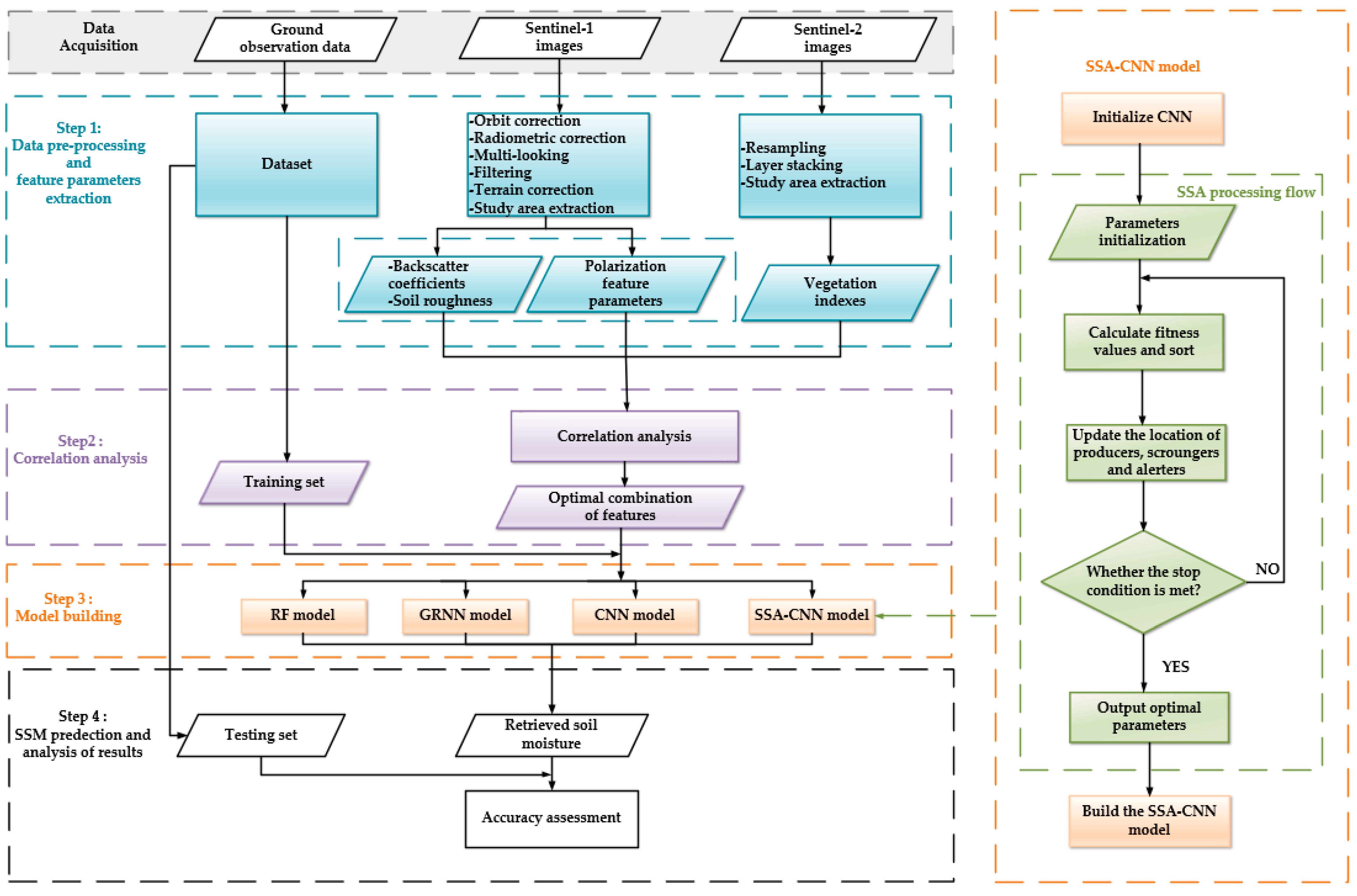
2.3. Methodology
2.3.1. Feature Parameters Extraction
- Feature Parameters Extracted from SAR Data
- Feature Parameters Extracted from Optical Images
2.3.2. Correlation Analysis between Input Parameters and Field Measured SSM Data
2.3.3. Establishment of the Models
- Traditional Machine Learning Models
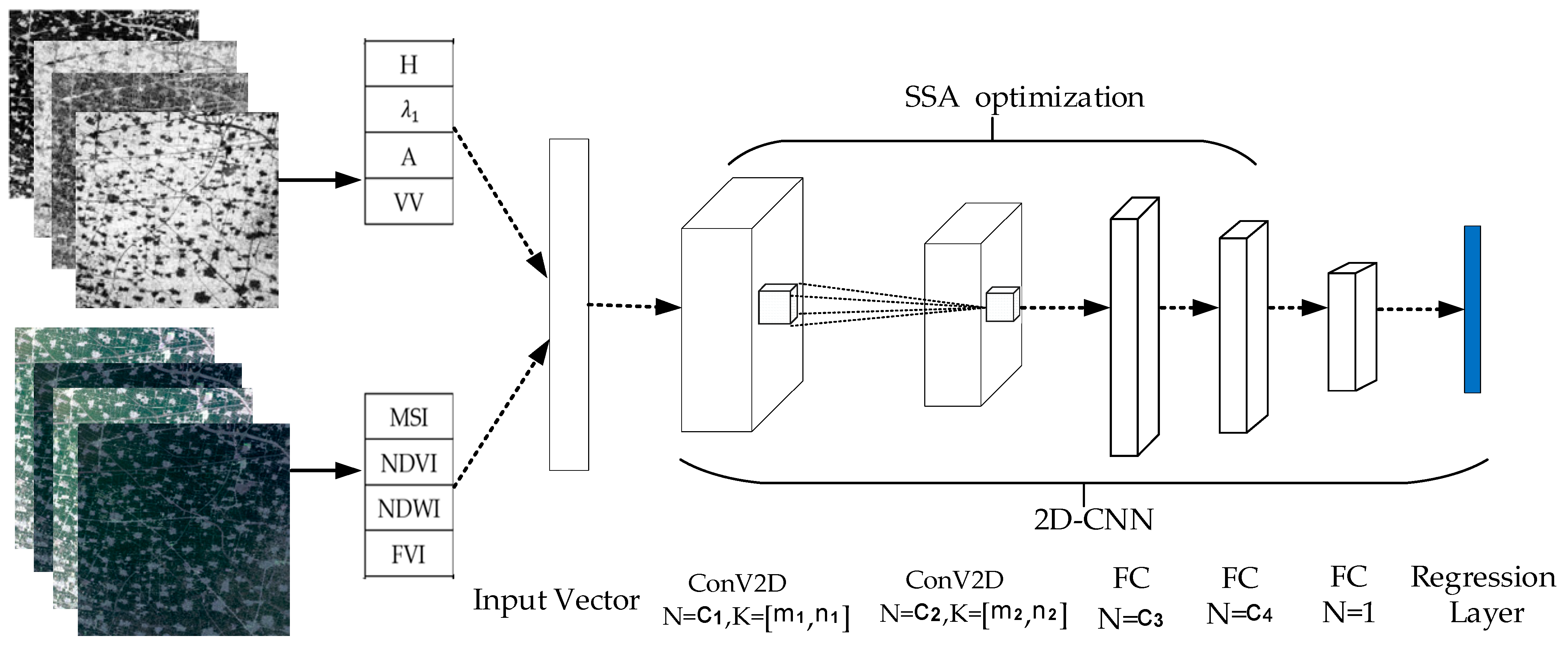
- Convolutional Neural Network Model
- Implementation of SSA-CNN
3. Results
3.1. Correlation Analysis Results
3.2. Hyper-Paramzeters Optimization Results after SSA
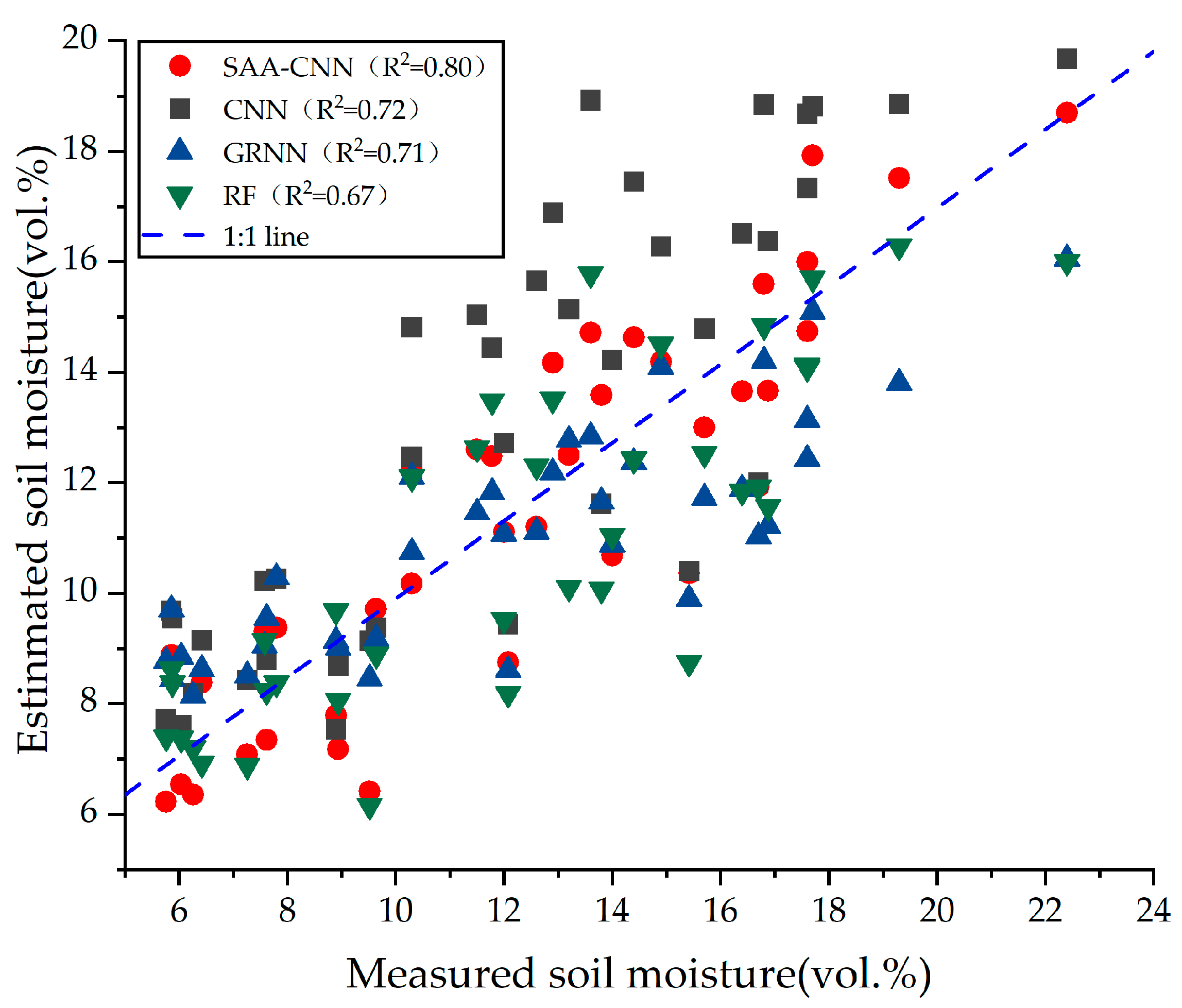
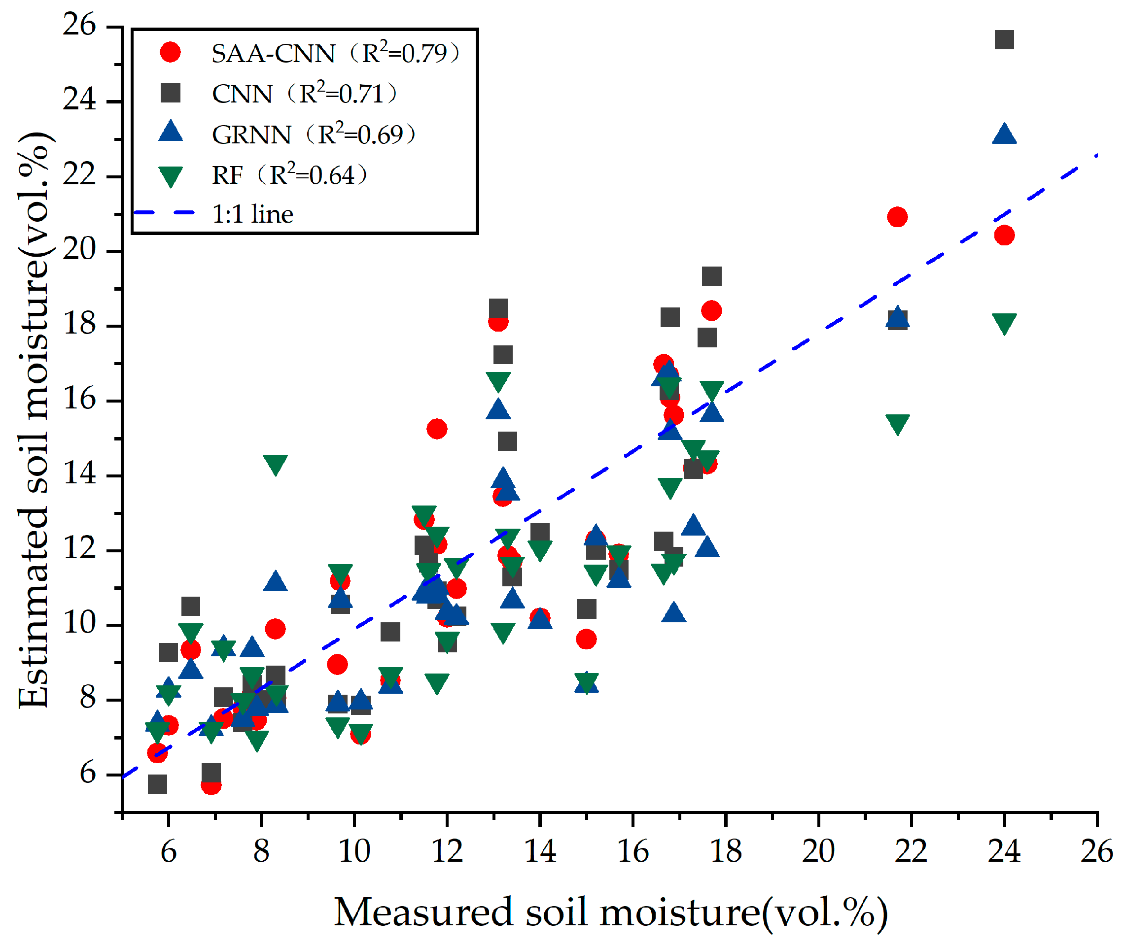
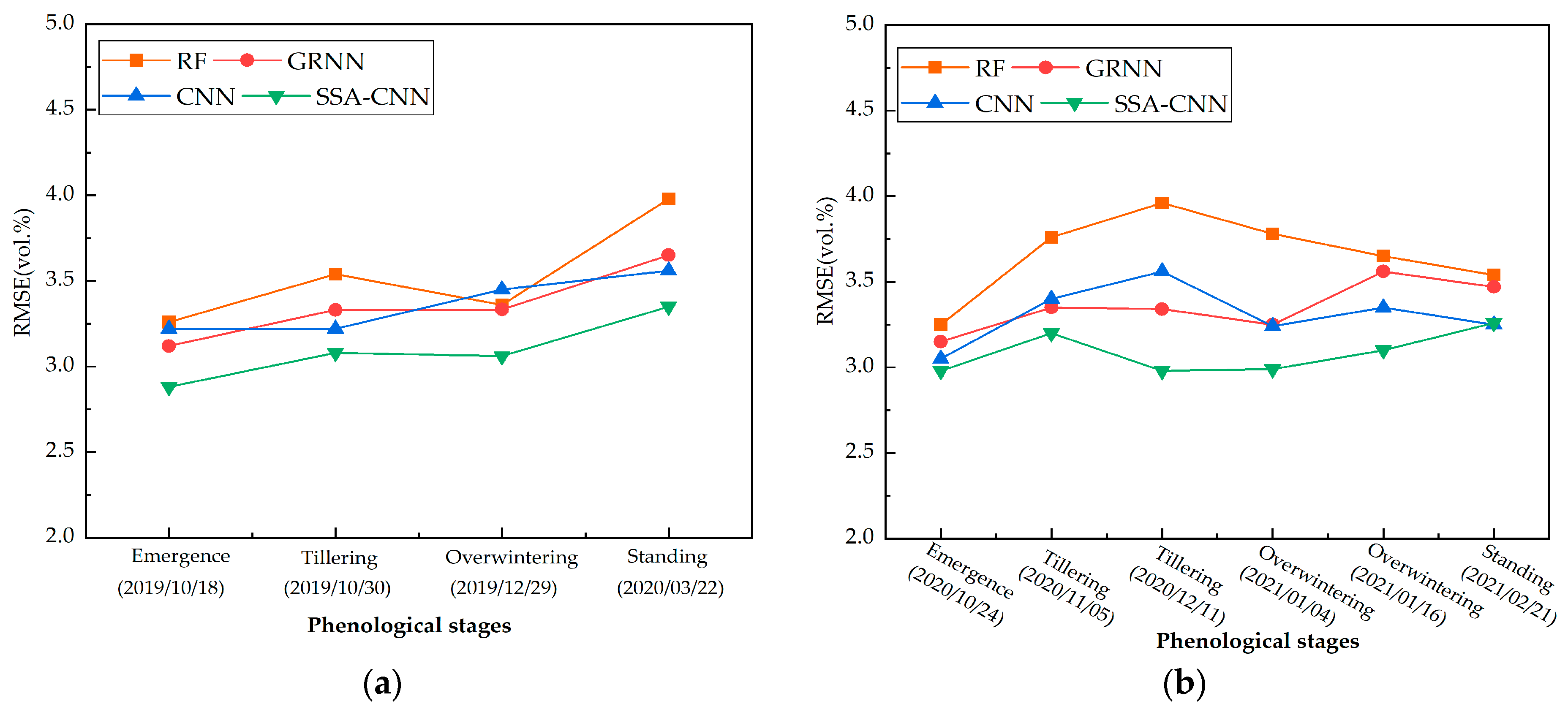
3.3. Regression Model Results and Analysis
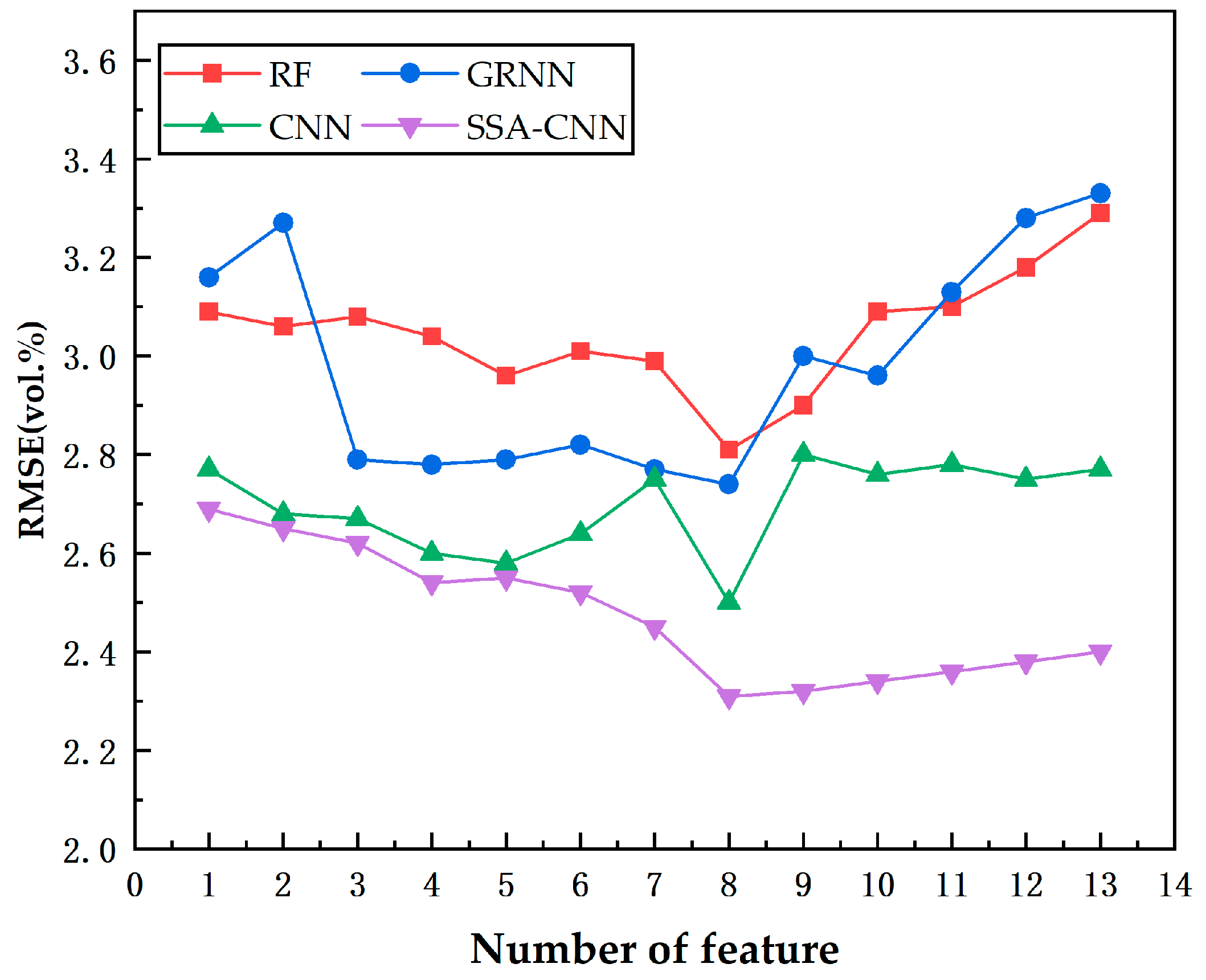
3.4. Performance of the Four Models with Different Number of the Feature Parameters
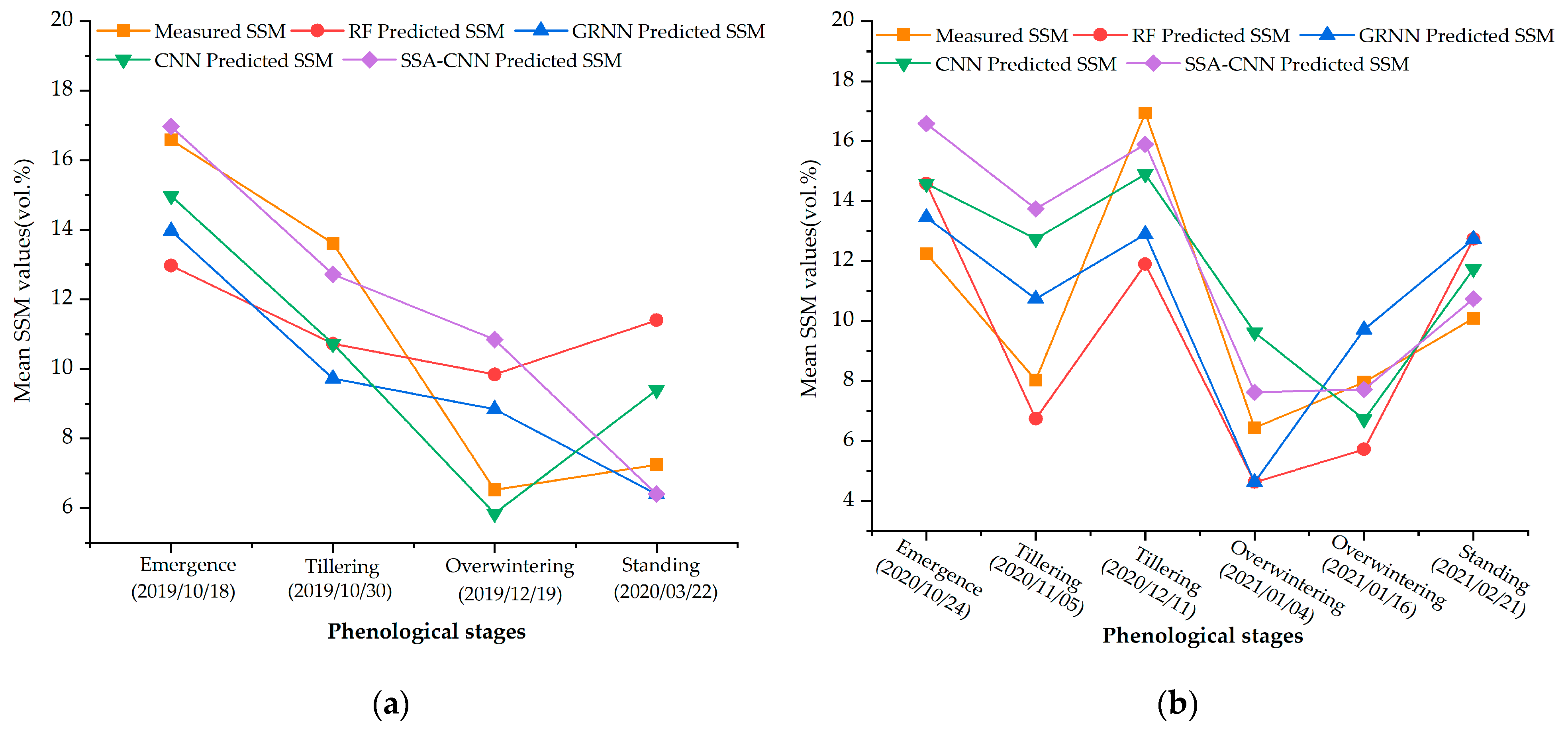
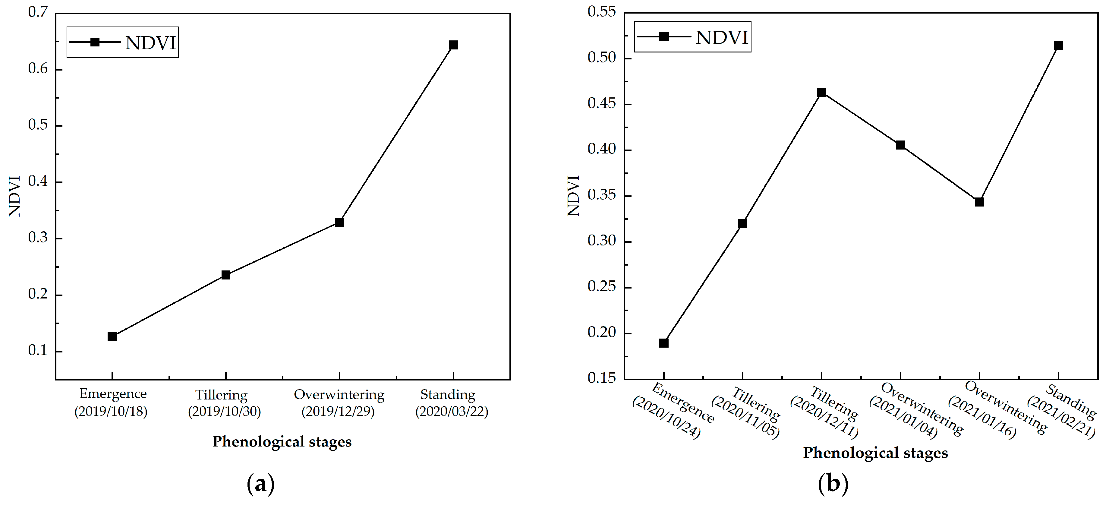
3.5. Analysis of Soil Moisture Dynamic Changes
3.6. Performance of SSM Estimation under Different Coverages of the Winter Wheat Plants
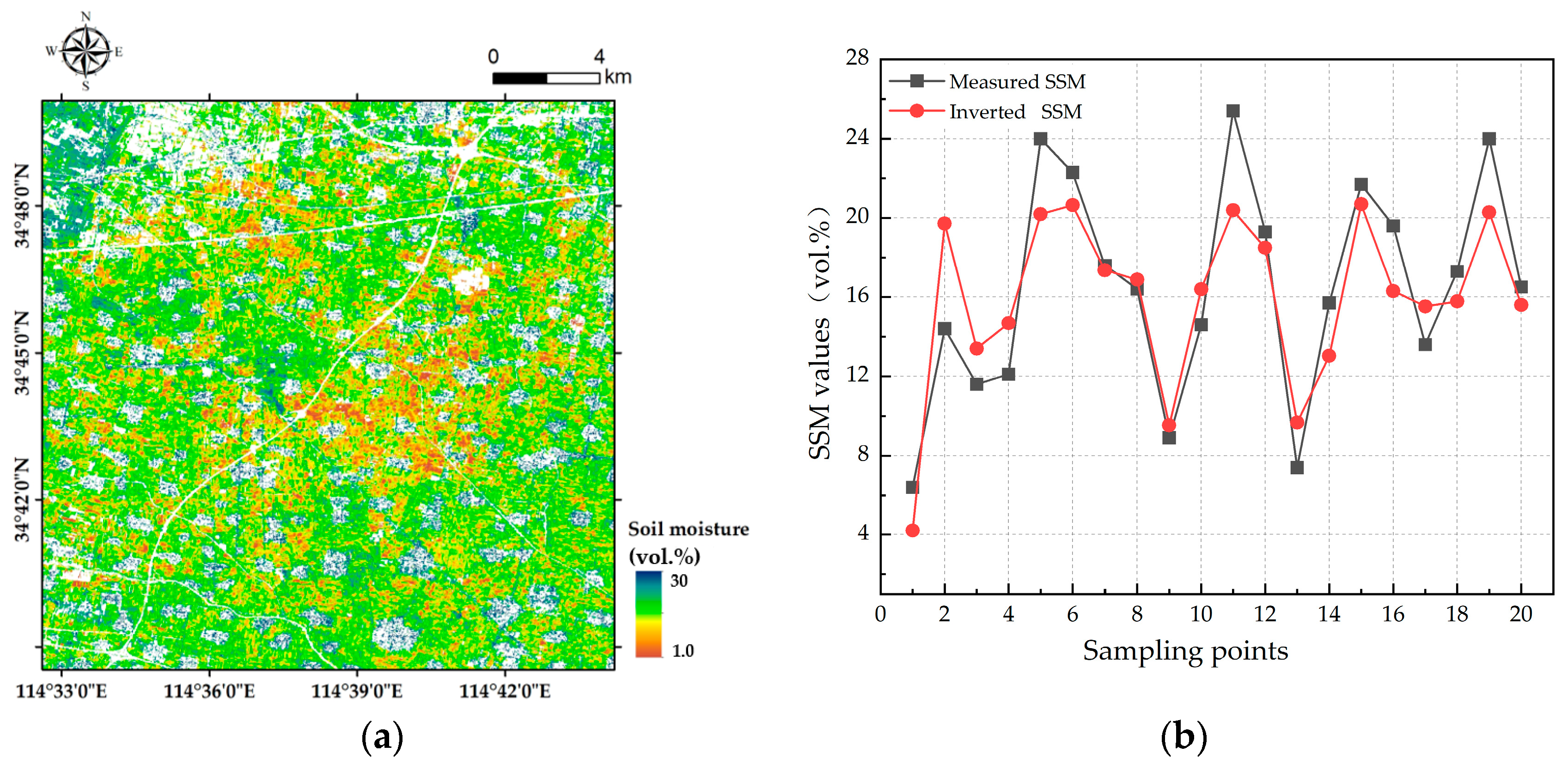
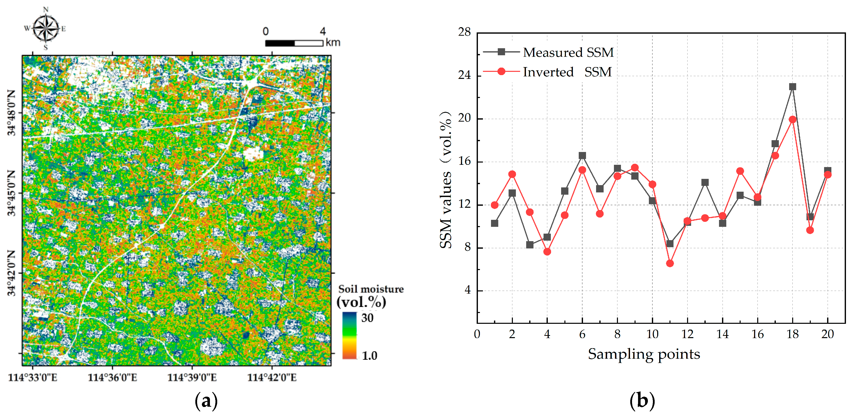
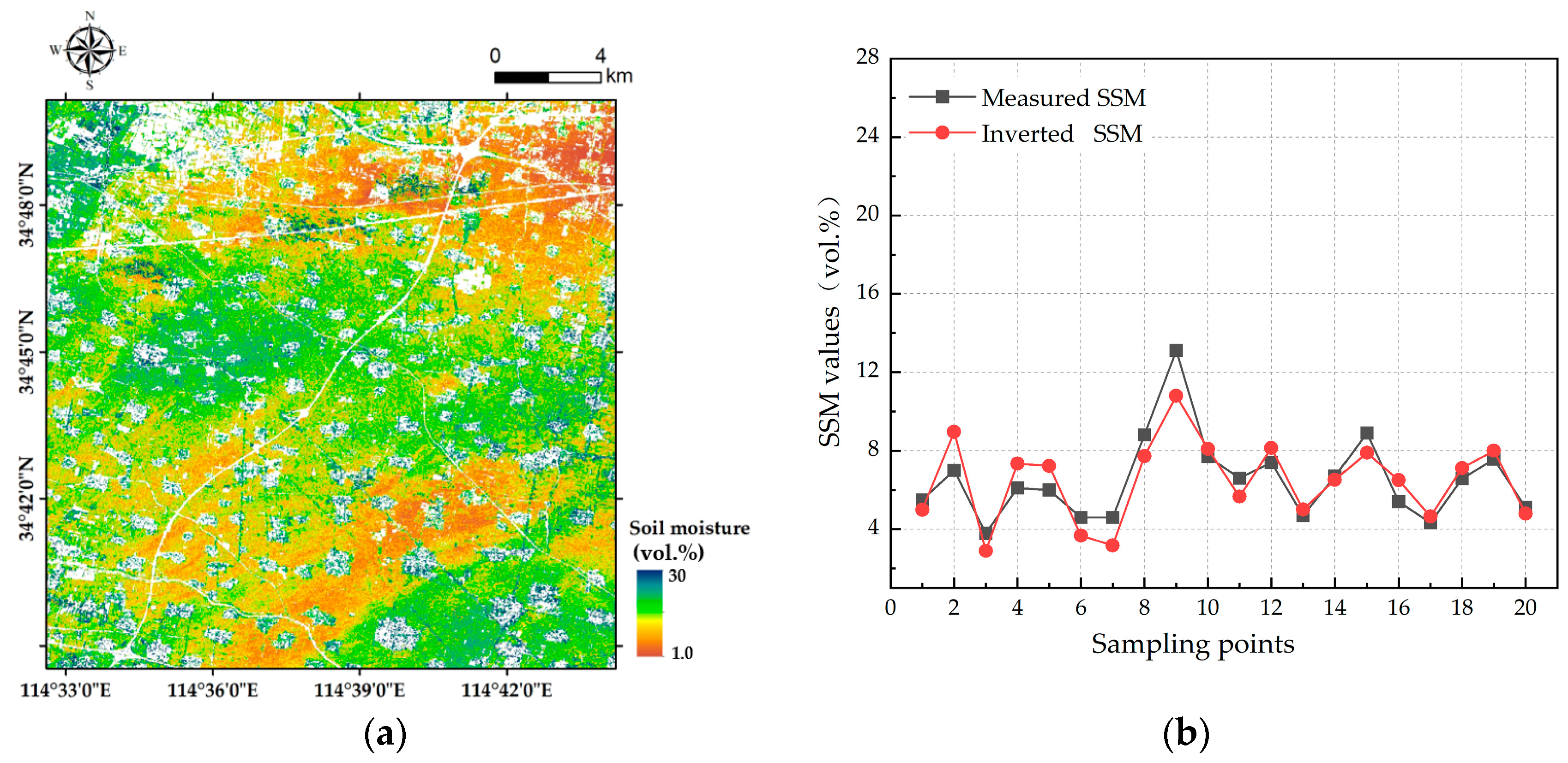
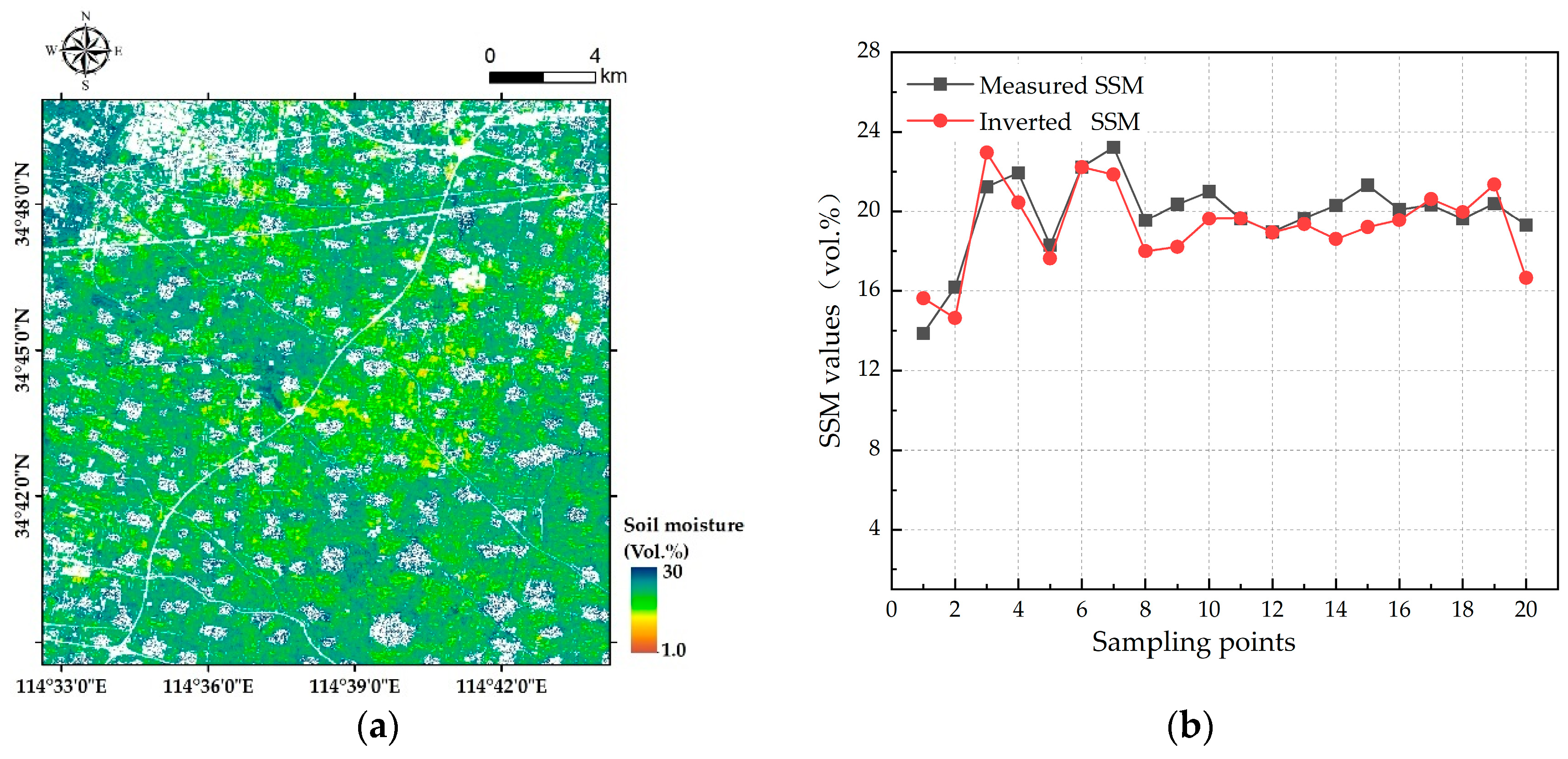
3.7. Results of the Regional SSM Inversion
4. Discussion
5. Conclusions
- (1)
- In total, 14 feature parameters related to SSM were extracted from Sentinel-1 and Sentinel-2 remote sensing data. After correlation analysis between 13 extracted feature parameters and field measured SSM by using Pearson correlation analysis and mutual information methods, 8 feature parameters, which were , FVI, NDVI, MSI, NDWI, H, VV, and A, were selected as the optimal combination of feature parameters for SSM inversion.
- (2)
- The SSA-CNN model was established and compared with RF, GRNN, and CNN models to validate its effectiveness. Among the four models, the proposed SSA-CNN model had a higher inversion accuracy. Its average , average RMSE, and average MAE were 0.80, 2.17 vol.%, and 1.68 vol.%, respectively.
- (3)
- The proposed SSA-CNN model was used to retrieve the regional SSM in winter wheat farmlands during four phenological stages. The findings indicated that the proposed method was feasible and suitable for SSM inversion in winter wheat covered areas, which provided a beneficial exploration and technical support for SSM estimation in agricultural regions.
Author Contributions
Funding
Data Availability Statement
Acknowledgments
Conflicts of Interest
References
- Guo, J.; Liu, J.; Ning, J.F.; Han, W.T. Construction and validation of farmland surface soil moisture retrieval model based on sentinel multi-source data. Trans. Chin. Soc. Agric. Eng. 2019, 35, 71–78. [Google Scholar]
- Gao, F.; Wang, J.M.; Sun, C.Q.; Wen, J. Progress in microwave remote sensing of soil moisture. Remote Sens. Technol. Appl. 2001, 16, 97–102. [Google Scholar]
- Zhang, X.; Chen, B.Z.; Zhao, H.; Wang, L. Based on time series Sentinel-1A data detection and analysis of farmland soil moisture change. Remote Sens. Technol. Appl. 2017, 32, 338–345. [Google Scholar]
- De Roo, R.D.; Du, Y.; Ulaby, F.T.; Dobson, M.C. A semi-empirical backscattering model at L-band and C-band for a soybean canopy with soil moisture inversion. IEEE Trans. Geosci. Remote Sens. 2001, 39, 864–872. [Google Scholar] [CrossRef]
- Verhoest, N.E.; Lievens, H.; Wagner, W.; Álvarez-Mozos, J.; Moran, M.S.; Mattia, F. On the soil roughness parameterization problem in soil moisture retrieval of bare surfaces from synthetic aperture radar. Sensors 2008, 8, 4213–4248. [Google Scholar] [CrossRef]
- Marzahn, P.; Ludwig, R. On the derivation of soil surface roughness from multi parametric PolSAR data and its potential for hydrological modeling. Hydrol. Earth Syst. Sci. 2009, 13, 381–394. [Google Scholar] [CrossRef]
- Yu, F.; Zhao, Y.S.; Li, H.T. Active passive remote sensing collaborative retrieval of soil moisture based on genetic BP neural network. J. Infrared Millim. Waves 2012, 31, 283–288. [Google Scholar] [CrossRef]
- Sandholt, I.; Rasmussen, K.; Andersen, J. A simple interpretation of the surface temperature/vegetation index space for assessment of surface moisture status. Remote Sens. Environ. 2002, 79, 213–224. [Google Scholar] [CrossRef]
- Yang, J.H.; Chen, L.W.; Wang, Y.X.; Zhao, S.X. Inversion of soil moisture based on improved water cloud model. Technol. Innov. Appl. 2020, 10, 13–15. [Google Scholar]
- Al-Yaari, A.; Wigneron, J.P.; Ducharne, A.; Kerr, Y.; De Rosnay, P.; De Jeu, R.; Mialon, A. Global-scale evaluation of two satellite-based passive microwave soil moisture datasets (SMOS and AMSR-E) with respect to Land Data Assimilation System estimates. Remote Sens. Environ. 2014, 149, 181–195. [Google Scholar] [CrossRef]
- Zhu, J.; Tsang, L.; Liao, T.H. Remote Sensing of Deep Snow with C Band Radar Data: Volume and Surface Scattering. In Proceedings of the 2021 IEEE International Geoscience and Remote Sensing Symposium IGARSS, Brussels, Belgium, 11–16 July 2021; IEEE: Piscataway, NJ, USA, 2021; pp. 622–624. [Google Scholar]
- Zhang, M. Surface Soil Moisture Retrieval in Wheat Covered Area Using Multi-Temporal SAR and Optical Satellite Data. Master’s Thesis, China University of Mining and Technology, Xuzhou, China, 2021. [Google Scholar]
- Bai, X.J. Research on Methods for Soil Moisture Retrieval in Prairies Areas Based on Multi-Frequency and Multi-Polarization SAR Data. Ph.D. Thesis, University of Electronic Science and Technology of China, Chengdu, China, 2017. [Google Scholar]
- Wang, S.N.; Li, R.P.; Wu, Y.J.; Zhao, S.X.; Wang, X.Q. Soil moisture retrieval based on environmental variables and machine learning. Trans. Chin. Soc. Agric. Mach. 2022, 53, 332–341. [Google Scholar]
- Chen, L.; Xing, M.; He, B.; Wang, J.; Shang, J.; Huang, X.; Xu, M. Estimating soil moisture over winter wheat fields during growing season using machine-learning methods. IEEE J. Sel. Top. Appl. Earth Obs. Remote Sens. 2021, 14, 3706–3718. [Google Scholar] [CrossRef]
- Karthikeyan, L.; Pan, M.; Wanders, N.; Kumar, D.N.; Wood, E.F. Four decades of microwave satellite soil moisture observations: Part 1. A review of retrieval algorithms. Adv. Water Resour. 2017, 109, 106–120. [Google Scholar] [CrossRef]
- Petropoulos, G.P.; Ireland, G.; Barrett, B. Surface soil moisture retrievals from remote sensing: Current status, products & future trends. Phys. Chem. Earth 2015, 83, 36–56. [Google Scholar]
- Callens, M.; Verhoest, N.E.C.; Davidson, M.W.J. Parameterization of tillage-induced single-scale soil roughness from 4-m profiles. IEEE Trans. Geosci. Remote Sens. 2006, 44, 878–888. [Google Scholar] [CrossRef]
- Jagdhuber, T.; Hajnsek, I.; Papathanassiou, K.P. An iterative generalized hybrid decomposition for soil moisture retrieval under vegetation cover using fully polarimetric SAR. IEEE J. Sel. Top. Appl. Earth Obs. Remote Sens. 2014, 8, 3911–3922. [Google Scholar] [CrossRef]
- Hajnsek, I.; Pottier, E.; Cloude, S.R. Inversion of surface parameters from polarimetric SAR. IEEE Trans. Geosci. Remote Sens. 2003, 41, 727–744. [Google Scholar] [CrossRef]
- Ulaby, F.T.; Batlivala, P.P.; Dobson, M.C. Microwave backscatter dependence on surface roughness, soil moisture, and soil texture: Part I-bare soil. IEEE Trans. Geosci. Electron. 1978, 16, 286–295. [Google Scholar] [CrossRef]
- Oh, Y.; Sarabandi, K.; Ulaby, F.T. An empirical model and an inversion technique for radar scattering from bare soil surfaces. IEEE Trans. Geosci. Remote Sens. 1992, 30, 370–381. [Google Scholar] [CrossRef]
- Dobson, M.C.; Ulaby, F.T. Active microwave soil moisture research. IEEE Trans. Geosci. Remote Sens. 1986, 1, 23–36. [Google Scholar] [CrossRef]
- Shi, J.; Wang, J.; Hsu, A.Y.; O’Neill, P.E.; Engman, E.T. Estimation of bare surface soil moisture and surface roughness parameter using L-band SAR image data. IEEE Trans. Geosci. Remote Sens. 1997, 35, 1254–1266. [Google Scholar]
- Ulaby, F.T.; Sarabandi, K.; Mcdonald, K.Y.L.E.; Whitt, M.; Dobson, M.C. Michigan microwave canopy scattering model. Int. J. Remote Sens. 1990, 11, 1223–1253. [Google Scholar] [CrossRef]
- Attema, E.P.W.; Ulaby, F.T. Vegetation modeled as a water cloud. Radio Sci. 1978, 13, 357–364. [Google Scholar] [CrossRef]
- Bousbih, S.; Zribi, M.; Mougenot, B.; Fanise, P.; Lili-Chabaane, Z.; Baghdadi, N. Monitoring of surface soil moisture based on optical and radar data over agricultural fields. In Proceedings of the 2018 4th International Conference on Advanced Technologies for Signal and Image Processing (ATSIP), Sousse, Tunisia, 21–24 March 2018; IEEE: Piscataway, NJ, USA, 2018; pp. 1–5. [Google Scholar]
- El Hajj, M.; Baghdadi, N.; Zribi, M.; Bazzi, H. Synergic use of Sentinel-1 and Sentinel-2 images for operational soil moisture mapping at high spatial resolution over agricultural areas. Remote Sens. 2017, 9, 1292. [Google Scholar] [CrossRef]
- Tong, C.; Wang, H.; Magagi, R.; Goïta, K.; Zhu, L.; Yang, M.; Deng, J. Soil moisture retrievals by combining passive microwave and optical data. Remote Sens. 2020, 12, 3173. [Google Scholar] [CrossRef]
- Ali, I.; Greifeneder, F.; Stamenkovic, J.; Neumann, M.; Notarnicola, C. Review of machine learning approaches for biomass and soil moisture retrievals from remote sensing data. Remote Sens. 2015, 7, 16398–16421. [Google Scholar] [CrossRef]
- Grewal, D.S. A critical conceptual analysis of definitions of artificial intelligence as applicable to computer engineering. IOSR J. Comput. Eng. 2014, 16, 9–13. [Google Scholar] [CrossRef]
- Vasconcelos, L.; Kijanka, P.; Urban, M.W. Viscoelastic parameter estimation using simulated shear wave motion and convolutional neural networks. Comput. Biol. Med. 2021, 133, 104382. [Google Scholar] [CrossRef]
- Liu, J.; Xu, Y.; Li, H.; Guo, J. Soil moisture retrieval in farmland areas with sentinel multi-source data based on regression convolutional neural networks. Sensors 2021, 21, 877. [Google Scholar] [CrossRef]
- Song, X.; Tang, L.; Zhao, S.; Zhang, X.; Li, L.; Huang, J.; Cai, W. Grey Wolf Optimizer for parameter estimation in surface waves. Soil. Dyn. Earthq. Eng. 2015, 75, 147–157. [Google Scholar] [CrossRef]
- Rashedi, E.; Nezamabadi-Pour, H.; Saryazdi, S. GSA: A Gravitational Search Algorithm. Inf. Sci. 2009, 179, 2232–2248. [Google Scholar] [CrossRef]
- Poli, R.; Kennedy, J.; Blackwell, T. Particle swarm optimization. Swarm Intell. 2007, 1, 33–57. [Google Scholar] [CrossRef]
- Xue, J.; Shen, B. A novel swarm intelligence optimization approach: Sparrow search algorithm. Syst. Sci. Control Eng. 2020, 8, 22–34. [Google Scholar] [CrossRef]
- Cloude, S.R.; Pottier, E. An entropy based classification scheme for land applications of polarimetric SAR. IEEE Trans. Geosci. Remote Sens. 1997, 35, 68–78. [Google Scholar] [CrossRef]
- Tong, L.; Chen, Y.; Jia, M.Q. Mechanism of Radar Remote Sensing; Science Press: Beijing, China, 2014. [Google Scholar]
- Huang, S.; Tang, L.; Hupy, J.P.; Wang, Y.; Shao, G. A commentary review on the use of normalized difference vegetation index (NDVI) in the era of popular remote sensing. J. For. Res. 2021, 32, 1–6. [Google Scholar] [CrossRef]
- Liu, J. Soil Moisture Retrieval in Farmland Surface Based on Sentinel Multi-Source Remote Sensing Data. Master’s Thesis, Northwest A&F University, Yangling, China, 2020. [Google Scholar]
- Qi, J.; Chehbouni, A.; Huete, A.R.; Kerr, Y.H.; Sorooshian, S. A modified soil adjusted vegetation index. Remote Sens. Environ. 1994, 48, 119–126. [Google Scholar] [CrossRef]
- Zhao, X.; Wang, J.; Liu, S. Improved monitoring of vegetation water content by remote sensing with coupled radiative transfer model. J. Infrared Millim. Waves 2010, 29, 185–189. [Google Scholar] [CrossRef]
- Zhao, J.; Zhang, B.; Li, N.; Guo, Z. Synergistic inversion of soil moisture on winter wheat cover surface based on Sentinel-1/2 remote sensing data. J. Electron. Inf. Technol. 2021, 43, 692–699. [Google Scholar]
- McFeeters, S.K. The use of the Normalized Difference Water Index (NDWI) in the delineation of open water features. Int. J. Remote Sens. 1996, 17, 1425–1432. [Google Scholar] [CrossRef]
- Xiong, J.Z. Urban Stormwater Model Parameter Sensitivity Analysis and Calibration. Master’s Thesis, Shandong University, Jinan, China, 2016. [Google Scholar]
- Hu, Q.; Guo, M.; Yu, D.; Liu, J. Information entropy for ordinal classification. Sci. China Inf. Sci. 2010, 53, 1188–1200. [Google Scholar] [CrossRef]
- Specht, D.F. A general regression neural network. IEEE. Trans. Neural Networ. 1991, 2, 568–576. [Google Scholar] [CrossRef] [PubMed]
- Breiman, L. Random forests. Mach. Learn. 2001, 45, 5–32. [Google Scholar] [CrossRef]
- LeCun, Y.; Bottou, L.; Bengio, Y.; Haffner, P. Gradient-based learning applied to document recognition. Proc. IEEE 1998, 86, 2278–2324. [Google Scholar] [CrossRef]
- Zhong, L.; Hu, L.; Zhou, H. Deep learning based multi-temporal crop classification. Remote Sens. Environ. 2019, 221, 430–443. [Google Scholar] [CrossRef]
- Guo, J.; Bai, Q.; Guo, W.; Bu, Z.; Zhang, W. Soil moisture content estimation in winter wheat planting area for multi-source sensing data using CNNR. Comput. Electron. Agr. 2022, 193, 106670. [Google Scholar] [CrossRef]
- Fu, Y.Z. Study on Vegetation Index of Remote Sensing and Its Aplications. Master’s Thesis, Fuzhou University, Fuzhou, China, 2010. [Google Scholar]
- Baghdadi, N.; EL Hajj, M.; Zribi, M.; Fayad, I. Coupling SAR C-Band and Optical Data for Soil Moisture and Leaf Area Index Retrieval Over Irrigated Grasslands. IEEE J. Sel. T op. Appl. Earth Obs. Remote Sens. 2015, 9, 1229–1243. [Google Scholar]
- El Hajj, M.; Baghdadi, N.; Belaud, G.; Zribi, M.; Cheviron, B.; Courault, D.; Hagolle, O.; Charron, F. Irrigated grassland monitoring using a time series of terraSAR-X and COSMO-skyMed X-Band SAR Data. Remote Sens. 2014, 6, 10002–10032. [Google Scholar] [CrossRef]


| Acquisition Date of Sentinel-1 | Growth Stage | Wheat Height (cm) | SSM Range (Vol.%) |
|---|---|---|---|
| 18 October 2019 | Emergence | 0 | 6–25 |
| 30 October 2019 | Tillering | 0–5 | 8–23 |
| 29 December 2019 | Overwintering | 5–15 | 4–13 |
| 22 March 2020 | Standing | 24–48 | 2–20 |
| 24 October 2020 | Emergence | 0 | 7–27 |
| 5 November 2020 | Tillering | 2–8 | 3–23 |
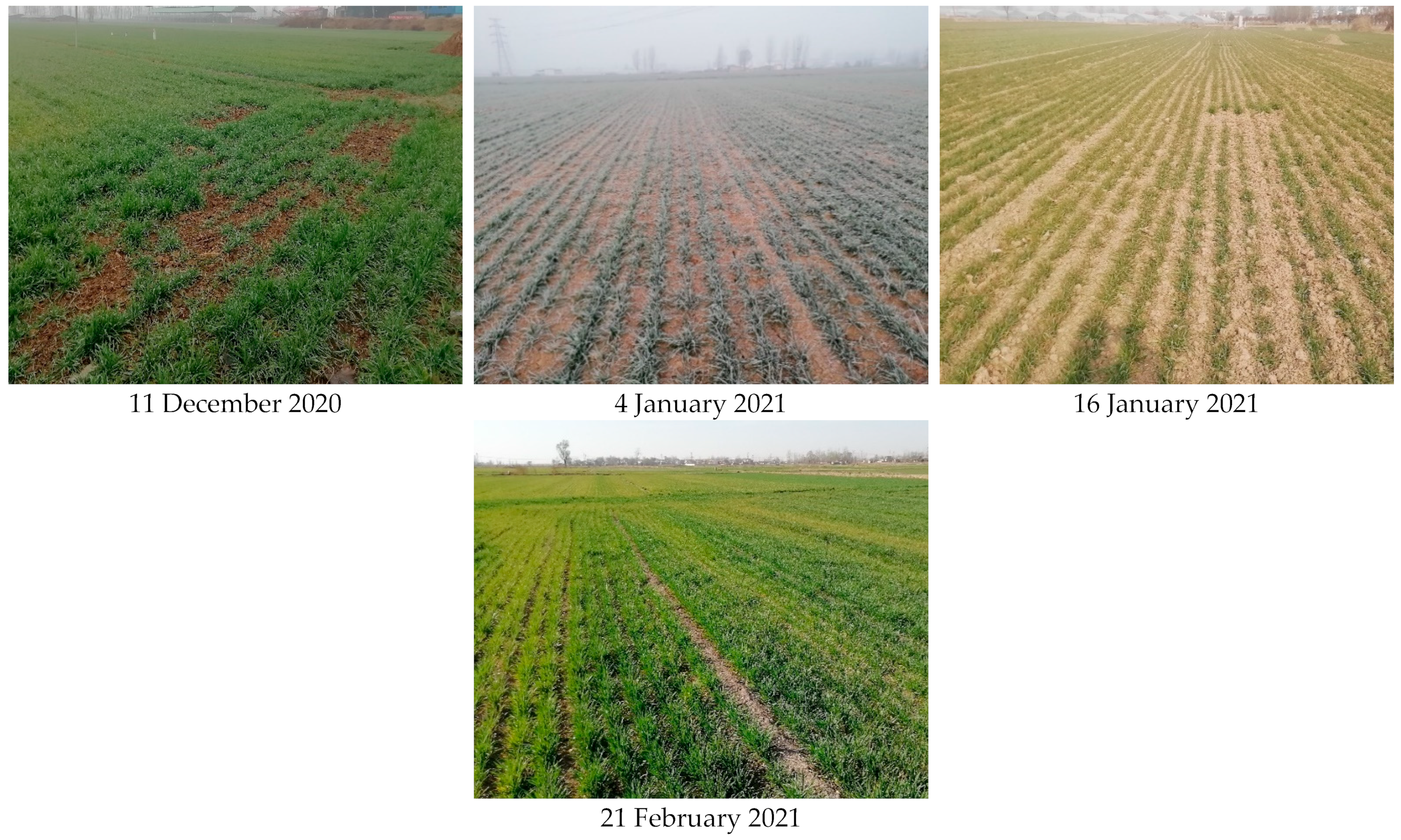
| 11 December 2020 | Tillering | 4–12 | 3–12 |
| 4 January 2021 | Overwintering | 6–16 | 9–29 |
| 16 January 2021 | Overwintering | 6–17 | 6–13 |
| 21 February 2021 | Standing | 11–21 | 6–19 |
| Acquisition Date of Sentinel-2 | Growth Stage | NDVI Range |
|---|---|---|
| 15 October 2019 | Emergence | 0.08–0.15 |
| 4 November 2019 | Tillering | 0.16–0.34 |
| 3 January 2020 | Overwintering | 0.16–0.45 |
| 23 March 2020 | Standing | 0.51–0.72 |
| 24 October 2020 | Emergence | 0.12–0.47 |
| 8 November 2020 | Tillering | 0.20–0.58 |
| 13 December 2020 | Tillering | 0.38–0.71 |
| 7 January 2021 | Overwintering | 0.24–0.65 |
| 17 January 2021 | Overwintering | 0.24–0.66 |
| 16 February 2021 | Standing | 0.39–0.72 |
| No. | Parameter | Note |
|---|---|---|
| 1 | Incident angle | |
| 2 | Backscatter coefficients | |
| 3 | ||
| 4 | Scattering entropy | |
| 5 | Inverse entropy | |
| 6 | Scattering angle | |
| 7 | Eigenvalues | |
| 8 | ||
| 9 | Surface roughness |
| Vegetation Index | Formulae | Reference |
|---|---|---|
| Normalized difference vegetation index (NDVI) | [42] | |
| Moisture stress index (MSI) | [43] | |
| Fusion vegetation index (FVI) | [44] | |
| Normalized difference water index (NDWI) | [45] |
| No. | Parameter | Correlation Coefficient |
|---|---|---|
| 1 | 0.491 ** | |
| 2 | −0.392 * | |
| 3 | −0.39 * | |
| 4 | 0.386 * | |
| 5 | −0.374 * | |
| 6 | −0.322 * | |
| 7 | 0.32 * | |
| 8 | 0.317 * | |
| 9 | −0.196 | |
| 10 | 0.172 | |
| 11 | −0.152 | |
| 12 | −0.126 | |
| 13 | 0.054 |
| No. | Parameter | NMI |
|---|---|---|
| 1 | 0.347 | |
| 2 | 0.231 | |
| 3 | 0.228 | |
| 4 | 0.222 | |
| 5 | 0.192 | |
| 6 | 0.191 | |
| 7 | 0.191 | |
| 8 | 0.184 | |
| 9 | 0.182 | |
| 10 | 0.172 | |
| 11 | 0.170 | |
| 12 | 0.165 | |
| 13 | 0.147 |
| Hyper-Parameter | First Training Set | Second Training Set | ||
|---|---|---|---|---|
| CNN | SSA-CNN | SSA-CNN | ||
| Learning rate | 0.01 | 0.006 | 0.004 | |
| Iterations | 40 | 51 | 49 | |
| Batchsize | 110 | 123 | 134 | |
| First layer | kernel size | 3 × 3 | 3 × 3 | 2 × 2 |
| First layer | number | 4 | 5 | 6 |
| Second layer | kernel size | 3 × 3 | 2 × 2 | 2 × 2 |
| Second layer | number | 8 | 12 | 12 |
| Number of neurons | 30, 30, 1 | 32, 23, 1 | 31, 26, 1 | |
| Model | First Testing Set | Second Testing Set | Average Accuracy | ||||||
|---|---|---|---|---|---|---|---|---|---|
| RMSE (Vol.%) | MAE (Vol.%) | RMSE (Vol.%) | MAE (Vol.%) | RMSE (Vol.%) | MAE (Vol.%) | ||||
| SSA-CNN | 0.80 | 2.11 | 1.65 | 0.79 | 2.22 | 1.71 | 0.80 | 2.17 | 1.68 |
| CNN | 0.72 | 2.53 | 2.09 | 0.71 | 2.57 | 2.05 | 0.72 | 2.55 | 2.07 |
| GRNN | 0.71 | 2.81 | 2.25 | 0.69 | 3.05 | 2.33 | 0.70 | 2.93 | 2.29 |
| RF | 0.67 | 2.83 | 2.46 | 0.64 | 3.12 | 2.61 | 0.66 | 2.98 | 2.54 |
Disclaimer/Publisher’s Note: The statements, opinions and data contained in all publications are solely those of the individual author(s) and contributor(s) and not of MDPI and/or the editor(s). MDPI and/or the editor(s) disclaim responsibility for any injury to people or property resulting from any ideas, methods, instructions or products referred to in the content. |
© 2023 by the authors. Licensee MDPI, Basel, Switzerland. This article is an open access article distributed under the terms and conditions of the Creative Commons Attribution (CC BY) license (https://creativecommons.org/licenses/by/4.0/).
Share and Cite
Wang, R.; Zhao, J.; Yang, H.; Li, N. Inversion of Soil Moisture on Farmland Areas Based on SSA-CNN Using Multi-Source Remote Sensing Data. Remote Sens. 2023, 15, 2515. https://doi.org/10.3390/rs15102515
Wang R, Zhao J, Yang H, Li N. Inversion of Soil Moisture on Farmland Areas Based on SSA-CNN Using Multi-Source Remote Sensing Data. Remote Sensing. 2023; 15(10):2515. https://doi.org/10.3390/rs15102515
Chicago/Turabian StyleWang, Ran, Jianhui Zhao, Huijin Yang, and Ning Li. 2023. "Inversion of Soil Moisture on Farmland Areas Based on SSA-CNN Using Multi-Source Remote Sensing Data" Remote Sensing 15, no. 10: 2515. https://doi.org/10.3390/rs15102515