

3PCD-TP: A 3D Point Cloud Descriptor for Loop Closure Detection with Twice Projection

1
College of Computer Science and Technology, Jilin University, Changchun 130012, China
2
School of Artificial Intelligence, Jilin University, Changchun 130012, China
3
College of Software, Jilin University, Changchun 130012, China
4
Key Laboratory of Symbolic Computation and Knowledge Engineering of Ministry of Education, Jilin University, Changchun 130012, China
5
State Key Laboratory of Automotive Simulation and Control, Jilin University, Changchun 130012, China
*
Author to whom correspondence should be addressed.
Remote Sens. 2023, 15(1), 82; https://doi.org/10.3390/rs15010082
Submission received: 23 October 2022
/
Revised: 8 December 2022
/
Accepted: 21 December 2022
/
Published: 23 December 2022
(This article belongs to the Topic Multi-Sensor Integrated Navigation Systems)
Abstract
:Loop closure detection (LCD) can effectively eliminate the cumulative errors in simultaneous localization and mapping (SLAM) by detecting the position of a revisit and building interframe pose constraint relations. However, in real-world natural scenes, driverless ground vehicles or robots usually revisit the same place from a different position, meaning that the descriptor cannot give a uniform description of similar scenes, failing LCD. Against this problem, this paper proposes a 3D point cloud descriptor with Twice Projection (3PCD-TP) for the calculation of the similarities between scenes. First, we redefined the origin and primary direction of point clouds according to their distribution and unified their coordinate system, thereby reducing the interference in position recognition due to the rotation and translation of sensors. Next, using the semantic and altitudinal information of point clouds, we generated the 3D descriptor 3PCD-TP with multidimensional features to enhance its ability to describe similar scenes. Following this, we designed a weighting similarity calculation method to reduce the false detection rate of LCD by taking advantage of the property that 3PCD-TP can be projected from multiple angles. Finally, we validated our method using KITTI and the Jilin University (JLU) campus dataset. The experimental results show that our method demonstrated a high level of precision and recall and exhibited greater performance in the face of scenes with reverse loop closure, such as opposite lanes.
1. Introduction
Over the recent years, one of the key autonomous driving technologies, simultaneous localization and mapping, has developed rapidly. The SLAM algorithm can provide prior maps for autonomous vehicles and is also the basis of localization and navigation. In SLAM systems, the odometry estimates or solves the current pose out of that in the previous frame through a recursive process. It follows the errors from the recursion pass on, hence accumulating frame by frame. Loop closure detection can detect whether a loop is created by using current sensor data and historical data and can then build interframe pose constraint relations, thereby eliminating the cumulative errors due to matching consecutive frames [1] and generating a higher-precision map. At present, autonomous driving systems have enormous application demands for reliable LCD algorithms. Accordingly, the research on LCD algorithms is of considerable significance.
The earliest application of LCD dates back to the vision-based SLAM [2,3]. Due to the higher-range accuracy of LiDAR than that of cameras, which is immune to both weather and illumination changes, LiDAR-based LCD methods have received high attention from researchers. Existing LiDAR-based LCD algorithms typically project the physical properties of point clouds onto a 2D plane, extract the handcrafted features, and then calculate the similarities according to the features to detect whether the current position has ever been visited. Examples include scan context (SC) [4], intensity scan context (ISC) [5], LiDAR Iris [6], and other methods, which segment point clouds into multiple subregions at a fixed distance and a fixed angle based on their polar coordinate system to project them onto a bird’s eye view (BV) image. While boosting efficiency, such dimension-reducing methods deprive point clouds of their original features on the z-axis and introduce a sequence problem of the mapping relations between 3D point clouds and 2D plane coordinates. More specifically, with the maximum height as a feature, SC can both detect a loop closure and provide the initial reference value for the angle of rotation for the SLAM algorithm while projecting 3D point clouds into a 2D descriptor. However, scan context is more vulnerable to changes in viewpoint because the height information of objects around the vehicle is susceptible to view and position changes. This means that the small range translation of the vehicle will bring the change of pixel values in the local scope of the descriptor. Small range translation means that the vehicle is translated within four meters in either the lateral or vertical direction. When the vehicle translates in the lateral or vertical direction, the relative position of the point cloud in the LiDAR coordinate system changes, which leads to different descriptors even at the same place. Additionally, during the encoding process, SC converts the problem of rotation in 3D space into a column-wise data sequence of 2D descriptors. As a result, the descriptors generated from different angles at the same place have to undergo similarity retrieval by brute-force matching. ISC uses intensity information instead of maximum height information. Although the reflection intensities of objects of the same material are theoretically the same, the intensity information would be interfered with by distance, incident angle, sensor noise, and other factors. Therefore, ISC fails to solve the inherent problems of such methods. LiDAR Iris encodes point clouds in 8-bit binary codes and attempts to estimate the rotation between two descriptors via Fourier transform, but the extracted features remain as height features. Iris attempts to estimate the rotation between two descriptors via the Fourier transform. Fourier transform is susceptible to noise, hence the unsatisfactory effect in detecting loop closures in real-world scenes. The above methods are limited in both the proper coordinating system of sensors and the dimension-reducing coding schemes. When the driverless system revisits the same place from a different angle or lane, or from another different position within the same lane, the relative positions of point clouds within the LiDAR coordinate system are caused to change. This would lead not only to the translational changes of rows and columns in the descriptors but also to the changes of pixel values in the descriptors. Furthermore, such coding schemes of projecting 3D point clouds onto a 2D plane using single height, intensity, and other properties could cause a huge loss of features, thereby reducing the abilities of the descriptors in describing and discriminating the same scene.
In order to endow the descriptors with robustness against the rotational and translational changes of sensors, we determined the primary direction and the origin of the point clouds in each frame employing Singular value decomposition (SVD), and after calculating the centroid of these point clouds, we redefined the coordinate system according to their distribution. To enhance the ability of the descriptor to describe scenes, we designed a 3D point cloud descriptor with a twice projection (3PCD-TP). We first mapped the pre-processed point cloud into a cylindrical coordinate system and then encoded the mapping result, starting with the principal direction. Meanwhile, we performed semantic segmentation on the point cloud to obtain the label of each point. The semantic information is encoded into the voxel of each bin of the 3D descriptor. In addition, since our descriptors are three-dimensional, we can preserve the height information of the point cloud in the z-axis dimension. Subsequently, we take advantage of the multidimensionality of 3PCD-TP to project it onto the xOz plane and the xOy plane, respectively, to produce its side-view and top-view projections. A loop closure constraint is built in the following way: We store the side-view projection of each point cloud frame into a KD Tree and select multiple candidates. We weight the Hamming distance of the side-view projection and the cosine distance of the top-view projection between the current frame and the candidates to measure the similarity between them. Lastly, we select the candidates that satisfy the threshold. The main contributions of this paper are listed as follows:
- A point cloud preprocessing approach has been introduced to weaken the rotational and translational effect of sensors. The origin and primary direction of cloud points have been redefined according to the distribution of point clouds, to render the new point cloud coordinates independent of the sensor coordinate system.
- The design of the 3D global descriptor 3PCD-TP combines semantic information and height information. Thereinto, the abilities of the descriptors in describing and discriminating scenes have been strengthened by using semantic information and equivoluminal multilayer coding schemes.
- A twice-projection-based weighted similarity algorithm has been proposed to measure the similarity between scenes in terms of the weighted sum of the Hamming distance of the side-view projection and the cosine distance of the top-view projection of the descriptors and to reduce the probability of loop closure mismatching.
The follow-up structure of this paper goes as follows: Section 2 elaborates on the related work to this study. Section 3 highlights the coding process and searching method of 3PCD-TP. Section 4 makes an evaluation over the dataset KITTI [7] and the self-collected campus dataset, and applies 3PCD-TP to the existing SLAM algorithm for mapping. Section 5 summarizes this paper’s current work and looks toward the follow-up work.
2. Related Work
2.1. Vision-Based LCD Algorithms
Currently, the LCD methods based on monocular, binocular, RGBD, structured light, 3D LiDAR, and other sensors have developed rapidly. Due to the compact arrangement and ease of processing and two characteristics of images, most vision-based LCD methods can extract image features directly from scenes, pinpoint the candidate positions using a bag of words (BoW), and calculate the similarity between distinct positions using the histogram. DBoW2 [8] first used BoW in vision-based LCD algorithms. They utilized the feature detection algorithm FAST to select features and generate BRIEF descriptors to construct a binary BoW. ORB-SLAM2 [9] utilized ORB features to generate a BoW and used a norm to measure the similarity score between the current and historical frames. M et al. [2] showed that Normal Distribution Transform (NDT) based features can capture enough structures and match images to features. VINS-Mono [10] chose to introduce a two-step geometrical verification method and triangulated visual features, thereby comparing their similarity. Vision-based loop closure detection methods have a great advantage in identifying objects because of the excellent imaging capability of cameras. However, the camera is susceptible to external light and environmental changes [6,11]. This may lead to changes in the brightness of the pixels of images, which to some extent affects the extraction of visual features and can lead to a failure in the place recognition.
2.2. LiDAR-Based LCD Algorithms
Compared to cameras, LiDAR is not sensitive to the changes in external ambient light. It has a wider detection range and a higher accuracy at long distance. In addition, LiDAR can obtain accurate three-dimensional information [12,13] compared to cameras. Therefore, LiDAR-based loop closure detection has received continuous attention due to its robustness to environmental changes and its high accuracy of localization. Usually, LiDAR-based LCD methods can be roughly generalized as local and global descriptors, depending on the means by which they extract features.
Local descriptors usually extract key points from the point clouds in each frame using a corner detector, separate the points near the key points, calculate the local features, and match the current and historical frames with BoW. For example, Scovanner’s 3D-SIFT [14] and J. Knopp’s 3D-surf [15] generated local descriptors by extracting key points from point clouds and matching them. Sivic et al. [16] generated cylindrical coordinates corresponding to each key point and then encoded the cells that segmented out of its nearby points into a histogram. S. Salti et al., proposed a feature descriptor SHOT based on 3D point clouds [17] and generated a local descriptor by extracting the key points and a normal from them. S. M. Prakhya et al., modified SHOT into B-SHOT [18], with each sector expressed in terms of the cosine of the angle between one feature point and its nearby point. J. Guo [19] utilized the intensity field returned by LiDAR sensors to construct an intensity-increasing 3D key point descriptor ISHOT. However, the interior structure of the scenes cannot be provided by extracting local descriptors directly to build a histogram, which is prone to matching errors in the face of highly repeated key points. The global descriptor in [20] extracted features from the geometrical relationship between point clouds to facilitate a fast retrieval of loop closure from the global map. Compared to local descriptors, global descriptors do without extracting corner points from mass point cloud data, which greatly shortens the time. For instance, the fast point feature histogram (FPFH) [21] used a normal to construct the histogram of point clouds and effectively described the local geometrical structure near point clouds, but it is inefficient in computational terms. ESF [22] generated a global descriptor according to three distinct shape functions of a point cloud’s surface distance, angle, and area distribution. M2DP [23] projected point clouds onto multiple planes, divided each plane into standalone storage cells by radius and azimuthal angle, and compressed the descriptors by SVD. SegMatch [24] divided point clouds into different sectors, extracted their features, and matched the corresponding elements by the random forest algorithm. SegMap [25] extracted the data-driven descriptors using a convolutional neural network [26] and identified the segmented point clouds using semantic information. However, these above global descriptors are lacking adequate rotation- and shift-invariances, and it is hard to abstract with accuracy the features of point clouds in the current frame.
Among the existing methods, the one with the best overall performance is the projection-based method to generate global descriptors. The procedure begins by mapping point clouds onto a 2D picture. Next, a descriptor is constructed by extracting the geometric feature vector, thereby quickly screening multiple candidate pictures. Finally, the most similar frames that satisfy the threshold are selected as the loop frames. For example, Kim et al. [4] extracted a 2D global descriptor named scan context from the BV images of LiDAR point clouds by using the maximum height feature. Seed [27] divided a certain number of point clouds into two layers for clustering and encoded the topological information about the segmented objects to generate a global descriptor. However, it is difficult for this method to identify the current position with exactitude when there are a small number of segmented objects. What the above two LCD methods adopt while encoding is the basic point cloud information, with quite a limited ability in describing scenes. Li et al. [28] introduced the semantic information instead of the height information about point clouds for global encoding and introduced the global semantics ICP to improve the matching performance in the algorithm. All projection-based global descriptors mentioned above project the point cloud onto the ground plane. This downward projection provides a better description of the current scene and summarizes the features of the current region. However, the above descriptors encode the projection results into a matrix for determining similarity. In this process, if the vehicle visits the same location from different directions or undergoes a translation, a row or a column offset will occur during the projection from a point cloud to a descriptor. This is because the above methods fail to unify the initial coordinate system. These offsets will eventually affect the effect of loop closure detection.
2.3. Motivation of This Work
The foregoing review and analysis identifies two limitations in the existing LiDAR-based LCD methods. First, the rotation and translation of sensors could make a difference in the consistency of the generated descriptors. Second, encoding is performed by dimension-reducing means, leading to the loss of mass information about the original point clouds and thus, lowering the degree of distinction between descriptors. Therefore, in order to upgrade the performance of LCD algorithms, on the one hand, we need to transform point clouds from the sensor coordinate system to the coordinate system based on the intrinsic distribution characteristics of point clouds to eliminate the impacts of rotational and translational changes. On the other hand, in the process of projecting the point cloud, a kind of 3D global descriptor is generated, and its dimension in the z-direction can extract the point cloud features in the vertical direction and preserve the semantic information of the point cloud. Compared to two-dimensional descriptors, our method can store slightly more information. Using the multidimensionality of descriptors, their ability to discriminate between scenes can be promoted in light of the degree of similarity between projections in different directions. On this basis, this paper proposes the 3D global descriptor 3PCD-TP and the method to calculate its similarity.
3. Methods
3.1. Algorithm Overview
This section presents our method in three aspects: preprocessing of point clouds, encoding and projection of 3PCD-TP, and similarity scoring. The pipeline of our proposed framework is shown in Figure 1. First, we semantically segment the point cloud to obtain the semantic information of the point cloud by obtaining the label of each point. To unify the coordinate system of the point cloud, we find the center of mass of the point cloud and use SVD to obtain the principal direction. We perform SVD on the covariance matrix of each frame of the point cloud to obtain the new origin and principal direction, to establish the new coordinate system of the point cloud. Subsequently, encoding is performed regarding the height and semantic information about the point clouds to generate 3PCD-TP. On this basis, the descriptor undergoes a side-view projection (onto the xOz plane) and a top-view projection (onto the xOy plane) to give two 2D images. Next, the side-view projection is stored in vector form in a KD tree for the preliminary search of a potential candidate frame. Finally, the weighted distance between the two projections of the current frame and the candidate frame is calculated as the similarity score between both frames for the judgement of whether a loop closure is constituted.
3.2. Preprocessing of Point Clouds
The preprocessing involves two steps. The first step is to acquire semantic information via SPVNAS [29]. The second step transforms the coordinates of point clouds using the primary direction provided by SVD and the calculated centroid of point clouds to weaken the interference to LCD introduced from the rotation and translation of sensors.
3.2.1. Acquisition of Semantic Information
During the process of data collection, it is inevitable to record pedestrians, vehicles, and other dynamic objects [30,31] into data. However, descriptors generated at similar positions could lead to significant differences in local pixel values due to the existence of such dynamic objects. Therefore, we classify the objects in point clouds via the semantic information and introduce dynamic scores hereinbelow to rule out the dynamic objects in point clouds. A voxel-based lightweight semantic segmentation model SPVNAS is selected in this paper to acquire semantic information. We feed the original point clouds into the pre-trained model to acquire the semantic information about each of them. We manually set the priority of different semantics to show their representativeness. We believe static objects in the scene are more representative. Figure 2 compares the original point clouds with those from which semantic information has been extracted. On the left are the original point clouds colored in terms of the intensity value; on the right are the semantic point clouds colored in terms of the species of the represented objects.
3.2.2. Unified Coordinate Axis
When a driverless vehicle revisits a region that it has ever visited from a different angle or lane, or from another close position within the same lane, the positions of all objects in the scene under the sensor coordinate system are changed with the changes in the vehicle’s position and pose. This will disenable the descriptor to give a uniform description of the same scene. To fix the above problem introduced by translation, we first calculate the centroid of point clouds and then translate the origin of point clouds p in each frame to their centroid position. Outliers, which would appear while LiDAR is scanning through the point clouds, could affect the accuracy in calculating the centroid of the point clouds. Therefore, the average Euclidean distance between each point in p and m adjacent points within its neighborhood is calculated by Formula (1). By assuming that the distribution of the results is a Gaussian distribution with mean and standard deviation, one can deem as outliers and filter from the point clouds the points for which the average distance goes beyond the interval defined by the global mean distance and the standard deviation, namely the points beyond the given threshold. Else, if falls within the range of the threshold, then will be saved. The range of the threshold is defined by Formula (2).
where is the global mean distance of point clouds, is the standard deviation of global mean distance, and is the coefficient of the standard deviation.
Furthermore, the point clouds at lower positions, such as the ground points, could interfere with the centroid calculation. We filter the point clouds below the height ( = 0.5 m in this paper) in the z-axis. After screening, the center-of-mass coordinates of the point clouds are used as the new origin for the holistic translation of the other points. Thus, even though the driverless vehicle has translated a certain distance in an arbitrary distance over the visited region, the similarity between descriptors would not be greatly affected.
where means the centroid of point clouds and is what the point clouds have been transformed into, with the point as the origin of the coordinate system.
During the loop closure detection of real-world scenes, vehicles inevitably revisit the same place from different angles. This causes the coordinates of the point cloud to change at the sensor coordinate system. In the process of encoding descriptors, this rotation will change the order of the descriptor in column, affecting the performance of LCD. To solve the above problem, we assign a uniform coordinate system to the point cloud. The principal direction of this coordinate system is only related to the distribution of the point cloud and is independent to the direction of the sensor’s coordinate system. In order to reduce the interference between sensor rotation and descriptor generation, we introduce the SVD to solve the covariance matrix and thus, find the principal direction of the point cloud for each frame. SVD is close to the idea of PCA in solving a single principal direction. The core idea of it lies in projecting the point cloud in three dimensions onto a plane to discover its principal direction [32,33,34,35]. The plane is chosen based on the distribution of points with the maximum variance. A plane with a more scattered distribution has a larger variance and is more informative. The calculation is as follows: firstly, we obtain the covariance matrix for the point cloud , and subsequently obtain the principal direction of this matrix by SVD.
Through analysis of the SVD result, we can obtain the principal axis of the point clouds. However, there are two cases of it: positive and negative. Accordingly, we need to vote the remaining points, count the points in the two opposite directions, and take the direction with more points as the final principal direction of the point clouds in the frame. Then, we can calculate the rotation matrix between the sensor coordinate system and the new coordinate system and rotate the point clouds to the given coordinate system. Thanks to the principal direction by means of SVD, even if the vehicle is rotated in the same position, we can still obtain a point cloud in a uniform principal direction, which attenuates the effect of the rotation of the sensor. The procedure of preprocessing is shown in Algorithm 1.
| Algorithm 1 Preprocessing Algorithm |
| Input: raw point cloud data ; Output: point cloud after preprocessing ; Algorithm:
|
3.3. Construction and Twice Projection of Descriptors
3.3.1. Construction of Descriptors
In order to characterize point clouds more accurately, we design 3PCD-TP for LCD. First, we divide the point clouds into regions. As shown in Figure 3, given a frame of point clouds, first they are mapped onto the cylindrical coordinate system, and then segmented at an angular resolution into equiangular sectors. Each sector is divided further at a length of in the radial direction. Furthermore, given that most projection-based descriptors are centered at the position of LiDAR, the space is divided into a radial sector with constant angle, distance, and height. At equal , the sector would be divided into multiple bins with unequal areas, small in proximity and large at a distance. One feature is selected for each bin, so that a single feature at a distance can represent large-area regions while that in proximity can only represent small-area regions. As a result, a difference in the representativeness of point clouds in each region will appear, hence affecting the encoding result. Therefore, a dynamic division method is designed in this paper to divide the sector in equal areas. The dividing procedure is shown in Figure 3a,b.
Subsequently, we divide the point clouds evenly into blocks in the z-axis at a height resolution of . Thus, these point clouds are evenly segmented into bins with equal volume. These bins are denoted by , with which the point in them each is related by Formula (11). We transform the results into the 3D rectangular coordinate system. The results after segmentation are shown in Figure 3d.
where , , .
After completing the division of point clouds, it is time to perform feature selection and encoding for the point clouds in each bin to generate a tensor of size , namely the 3PCD-TP descriptor. In this paper, we choose to extract the height and semantic information about the point clouds to encode the descriptor. Since our descriptor is three-dimensional, it already contains the height information in the z-direction. We could save the semantic information about the point clouds within the region in the voxel value of each bin. We begin by making statistics of the semantics in each bin and single out the semantic value best representative of the region, i.e., the semantic value of the most significant number of points with the same semantics as the semantics of the bin. We use to save the semantic values in each bin which can represent the voxel of our 3D descriptor.
3.3.2. Twice Projection
In order to improve the efficiency of calculating the similarity between descriptors, we project 3PCD-TP twice in the side view direction and top view direction, thus downscaling to generate two sets of two-dimensional descriptors. Figure 4d,f shows the two two-dimensional sub-descriptors generated after twice projection of the 3D descriptor 3PCD-TP, where (d) is the result of the side-view projection and (f) is the result of the top-view projection. The part close to red in Figure 4 indicates that the height of the point cloud in the region is high, while the blue part indicates that the height of the point cloud in the region is below the ground or not observed due to occlusion.
The rotational invariance of the descriptors is challenged by the fact that the principal direction selected in the preprocessing stage, in very specific scenarios (e.g., when obscured by objects in the near vicinity), causes a small magnitude rotation of the principal direction of the descriptors in the same location. To strengthen the rotational invariance of our descriptors, we introduce the side-view projection of 3PCD-TP. During the first projection to the side direction, we project the data in the direction that preserves the annular data acquired from a round of LiDAR scanning. This ring-wise information does not change with rotation, which means that the projection has robust rotation invariance. During the side-view projection, we project the descriptor in the direction , and the result of this projection is called the ring key. We statistically determine the most frequent semantic values in the direction and assign them to as the pixel of each bin in the side-view projection.
where the symbol ‘’ represents the projection onto a 2D plane. represents a function that is used to obtain the label with the highest frequency in the label set. In formula (6), means a set of semantic labels. The ring key calculated from the above formula possesses rotation-invariance and saves the height and semantic information about the original point clouds. We make a preliminary search for the current frame according to the side-view projection result of 3PCD-TP, reading the pixels of the ring key on a column-wise basis, and converting them into a set of vectors to save in the KD tree for coarse search. Since the result of the primary projection retains the feature of the original point clouds, the number of candidate frames can be reduced appropriately. Therefore, this projection method slightly improves the efficiency of the initial search.
In the secondary projection, 3PCD-TP is projected to the direction, which is called the sector key. The frequent occurrence of moving dynamic objects during the driving process leads to a decrease in the accuracy of loop closure detection as well as positional estimation. So, we classify each point according to the semantic information and determine whether it is a dynamic object. If yes, a small weight is assigned to that point, which is called the dynamic score . indicates the expected weight that we anticipate in the computation. We introduce the concept of dynamic score for two reasons: to reduce the impact of dynamic objects on descriptor calculation [36], and to not completely deprive dynamic objects of their features and let them participate in the computation. We consider the information of dynamic objects as a kind of information and therefore, do not delete it completely. Each pixel in the sector key stores the dynamic height . We use Equation (9) to reduce the impact of dynamic objects on our scene recognition, rather than eliminating the presence of dynamic objects altogether. The reason for encoding the height information is also that this feature can better represent the structural information in the current scene. The dynamic height can be obtained by multiplying the dynamic score by the height in the projection direction (z-direction).
where means the set of points in row and column , means the set of the points’ height. This projection of 3D descriptors onto two groups of 2D descriptors proposed in this paper can preserve more point cloud features and better represent the point cloud of the current frame compared to a single 2D descriptor.
3.4. Generation of the Weighted Distance Function
To enhance the precision of descriptor similarity calculation, we adopt a calculation method using the weighted distance instead of the single distance. As shown in Figure 4e, we utilize the D-Hash algorithm, an image similarity algorithm used for binary encoding of the side-view projection result of 3PCD-TP. In our method, the D-Hash of each side-view projection is generated only once and is then stored. Only the Hamming distance between frames is calculated for the subsequent similarity calculation. The efficiency of D-Hash is higher than other similarity calculation algorithms in our method. If the pixel in a certain region of the side-view projection is greater than the pixel in its right-hand side regions, then the binary hash code for this region shall be set as 1, else 0, to generate a 2D matrix consisting only of 0 and 1. Using as the “fingerprint” of the side-view projection for coarse search, we finally retrieve N candidate frames most similar to the current frame.
We denote the 3PCD-TP of the current frame and the ith candidate frame by and , respectively, where was taken from the set {}. For the 3PCD-TP of the current and candidate frames, we make an initial attempt to use the cosine distance between their top-view projections as the result of fine search. However, the cosine distance turns out to be very sensitive to even a tiny displacement. The translational motion of a point of view could cause a dramatic decrease in cosine similarity. To evaluate the effect of LCD more accurately, a weighted distance function is proposed in this paper to weight the Hamming distance of the side-view projection and the cosine distance of the top-view projection of each descriptor. We denote the similarity between and by the weighted distance . The smaller the value of , the closer the distance, hence the higher the similarity between and , and the greater the possibility of forming a loop closure. The weighted distance can be calculated as below:
where: denotes XOR; and denote the binary values of the side-view projections of and , respectively, at the pixel point at the position (j, k); is the Hamming distance between and ; and are the vectors for the jth column under the secondary projections of and , respectively; is the weight. We use the Hamming distance of the primary projection and the cosine distance of the secondary projection to calculate the similarity of two frames of point cloud. These two approaches show the differences between descriptors from different projection angles. We select the frame with the minimum weighted distance as the closest candidate frame matching the current frame .
where γ is the threshold of distance used to judge whether a loop closure is constituted, the set N are the candidate frames retrieved from the cursory search through the KD tree. If the weighted distance between and is greater than the given threshold, then the corresponding frame would not be assumed as a loop frame. To avoid matching errors, we adopt ICP for registration of the closest candidate frame for which the weighted distance is smaller than the threshold. If the result in the algorithm is convergent, then it would be accepted as a right loop closure.
4. Experiments
This section elaborates on our experiments using the public dataset KITTI and another dataset collected from the Jilin University (JLU) campus and makes a comparison with the currently mainstream LCD methods such as SC [4], ISC [5], M2DP [23], and ESF [22]. All the above algorithms are implemented based on C++. In the method of this paper, the dimensions of the division of 3PCD-TP are set as = 60, = 20, and = 10, the angular resolution as = 6°, the z-axis resolution as = 0.5 m, and the number of nearest loop frames searched through the KD tree as 5. The 50 frames are set at the closest distance to the current frame to avoid being searched during loop closure search. All above experiments are conducted on a machine with mainboard ASUS Z9PE-D8 WS, CPU Inter Xeon E5-2680 v2 @2.20 Ghz*2, graphics card GTX1060, and 8 GB memory.
4.1. Experimental Results over the Public Dataset
4.1.1. Introduction to the Dataset KITTI
KITTI [7] Odometry is a classic public dataset widely applied in SLAM, visual odometry, and other tasks. A vehicle-borne 64-line LiDAR collected it (Velodyne HDL-64E), containing a total of 11 sequences (00–10) with the ground truth, among which the sequences containing loop closures are 00, 02, 05, 06, 07, 08, and 09; the sequences 00, 05, 06, 07, and 09 contain only unidirectional loop closures, the sequence 08 contains only reverse loop closures, and the sequence 02 contains both unidirectional and reverse loop closures. Figure 5 shows the regions of loop closure ground truth for sequences 00, 02, 05, 06, 07, and 08 in KITTI dataset. The obverse loop closure regions are marked by solid boxes, as shown in Figure 5a–e. In Figure 5b,f, the region marked with a dashed box is the reverse loop closure, where the vehicle revisits from the opposite direction.
4.1.2. P-R Curves over the Dataset KITTI
In order to weigh the LCD effectiveness in the algorithm in this paper, we calculate the precision (P) and recall (R) of 3PCD-TP and the other mainstream LCD methods over the public dataset and plot their P-R curves for comparison. Here, the precision refers to the probability that all loop closures detected by the algorithm are true ones, namely the ratio of the number of positive samples of the right loop closures to that of the detected loop closures; the recall refers to the probability that all true loop closures are detected to be the right ones, namely the ratio of the number of the positive samples that are detected to be the right ones to the number of all positive samples.
Figure 6 presents the P-R curves of our method and the four algorithms SC, ISC, M2DP, and ESF over the sequences 00, 02, 05, 06, 07, and 08 for the dataset KITTI. The larger the area enclosed between the P-R curve and the coordinate axis, the greater the effectiveness of LCD. Overall, the method in this paper exhibits the top performance in most of the sequences except for the sequence 06, as compared to the other four algorithms. The area covered under the P-R curve of the method ESF is the smallest in most cases, with P showing a significant downtrend with the increase of R. The method M2DP has quite an unstable behavior over these six sequences: it has excellent LCD effectiveness over all the sequences 00, 02, 05, and 06, but the curve shows an abrupt decline over the sequences 07 and 08. The main reason for the above phenomena is that neither the algorithm ESF nor M2DP possess a perfect rotation-invariance. When the sensors undergo a change in angle of view, a significant difference appears in the descriptors generated by them, thereby leading to the incidence of loop closure misdetection. Both SC and ISC demonstrate high level of performances in the graph, except that the main algorithmic difference between both is that the former uses maximum height, while the latter adopts intensity values for encoding. Over the four sequences 00, 05, 06, and 07 containing only unidirectional loop closures, these methods have the most similar effectiveness to the method proposed in this paper. However, over the sequence 02, there appears a significant gap between these two methods and ours. The main reason is that there are unidirectional loop closures and reverse ones in sequence 02. Both rotation and translation could change the column orders and local pixel values of the descriptors generated by them, affecting the precision of LCD. This effect is more obviously manifested over the sequence 08, which only contains reverse loop closures. However, the method in this paper had redefined the origin of coordinates and the principal axis direction of point clouds according to their distribution at the preprocessing stage of point clouds, mitigating the effects of vehicle rotation and translation on the encoding process. Therefore, it turns out with better LCD effectiveness and a greater area covered under the P-R curve in the face of the reverse loop closure scenes in the sequences 02 and 08.
4.1.3. Maximum F1-Score and EP Value Results over the Dataset KITTI
In addition to the P-R curve plots, we also use maximum F1-score and extended precision (EP) to weigh the performance of this algorithm quantitatively. Maximum F1-score is the harmonic mean of precision and recall, which is used to weigh the overall performance of LCD. A greater F1 value coincides with a greater effectiveness of LCD. EP is designed exclusively for LCD algorithms and is used to reflect the robustness of LCD methods. Maximum F1-score is defined as:
Extended precision is defined as:
where P is precision, R is recall, P0 is the precision at the minimum recall, and R100 is the recall at the maximum precision.
Table 1 lists the maximum F1-scores and EPs of different methods. Evidently, the F1-scores and EPs of 3PCD-TP are both higher than their counterparts of the other four mainstream methods over most of the sequences. The average maximum F1-score of our method is 0.947 over the dataset KITTI, approximately 7.5% higher than that (0.881) of SC, which has the best performance among the remaining algorithms. The average EP value of 3PCD-TP also reaches 0.857, approximately 11.6% higher than that (0.768) of the second-ranking method SC. Our methods’ F1-score and EP value are higher than their counterparts in the other four algorithms over the sequences 00, 02, 05, and 07. The F1-score is slightly lower than that in the algorithm SC over the sequence 06, but the highest EP value is maintained among the five algorithms. Our method has the highest F1-score over the sequence 08 but an EP value slightly lower than that in the algorithm ISC. The data in Table 1 quantitatively demonstrate that our proposed method is superior in performance and stability to the currently prevailing methods. This coincides with their behaviors in P-R curves, further showing the effectiveness of our proposed method.
4.2. Experimental Results over the Campus Dataset
4.2.1. Introduction to the Campus Dataset
The team JLUROBOT owns multiple data-collecting platforms that can be applied in data-collection tasks under different road conditions. Figure 7 displays some of such collecting platforms designed and set up by the team, among which the collecting platforms J5 and Avenger are dedicated to data collection in separate environments, such as mountains, forests, and cross-country roads. In order to verify the effectiveness of the algorithm in this paper when the sensors undergo a wide-angle rotation and a small-range translation, our team designs specific data collection routes and collects data from the campus environment using the mobile platform of Shanghai Volkswagen Tiguan, which is equipped with a rotation-type LiDAR VLP16 of Velodyne and an inertial navigation system (INS) npos220s. Figure 8 displays our vehicle and related devices. During the data collection process, the vehicle was traveling at a speed of 30 km/h, the LiDAR was collecting point cloud data at a frequency of 10 Hz, and the INS was collecting (longitude, latitude, and altitude) data at a frequency of 125 Hz, to provide the ground truth for LCD.
4.2.2. P-R Curves over the Campus Dataset
In order to verify the LCD effectiveness of our algorithm in real-world scenes, we collect four segments of data from the JLU campus. Among them, School-01 contains loop closure data of visiting a same position from different angles and lanes, the data of School-02 and School-04 contain multiple segments of reverse loop closures, and the data of unidirectional loop closures predominate School-03. The above four segments of data cover all possibilities of loop closures mentioned in the motivation of this paper. The four graphs in Figure 9 display the effectiveness of each algorithm over the four segments of data. Overall, the trends of P-R curves in all algorithms over the campus dataset of Jilin University are roughly the same as those over the dataset KITTI. The area covered under the P-R curve of our algorithm is the largest in whichever of the four graphs. The algorithms ESF and M2DP remain the poorest performing two of all, and the behavior of M2DP remains quite unstable. Both algorithms SC and ISC still keep good effectiveness in real-world scenes, and they are the two which have P-R curves similar to our algorithm. Specifically, over the segment of data School-03 containing only unidirectional loop closures, the effectiveness of SC and ISC is basically consistent with that of our algorithm over the sequences KITTI-00, 05, 06, and 07. The P-R curves of the three algorithms are quite similar, each covering a great area, while our algorithm is particularly outstanding. Over the data of School-02 and 04 containing only reverse loop closures, a gap starts to appear between the effectiveness of the algorithms SC and ISC and that of our algorithm, the same case as that over the sequence KITTI-08. Over the data of School-01, the behavior of our algorithm remains stable, with the P-R curve always residing on the top. From the perspective of data, it is a relatively simple problem to detect unidirectional loop closures in LCD tasks. The revisiting of the vehicle to a previously visited region is a continuous process. With no rotation but only small-range translation, the probability that similar point clouds will appear in two data fragments is very great. As long as the descriptor has good ability in describing scenes, it can still achieve satisfactory detection results even lacking adequate rotation- and shift-invariances, for example, SC and ISC. However, when the vehicle returns to the visited region from a different angle and/or a different lane (e.g., School-01, 02, and 04), rotation and translation do not change the distribution of the objects around the vehicle, but only change their positional relationship in the sensor coordinate system. At this moment, the descriptor is required to have the ability to keep the data content and structure unchanged or the ability to copy with rotational and translational changes. Evidently, the descriptor proposed in this paper has a stronger ability than all the other four algorithms in coping with such scenes.
4.2.3. Evaluation of Maximum F1-Score and EP Value
We conducted a quantitative analysis of the five algorithms still using maximum F1-score and EP value over the campus dataset. It is also evident from Table 2 that the average maximum F1-score of 3PCD-TP over the four segments of data is 0.922, 5.25% higher than that (0.876) of the second-ranking algorithm SC and 10.29% higher than that (0.836) of the third-ranking algorithm ISC. The average EP of our algorithm is 0.775, 15.50% higher than that (0.671) of SC and 16.37% higher than that (0.666) of ISC. In the dataset School-03, our method has a very close F1-score and an EP value to their counterparts of SC and ISC, indicating that all these three solutions demonstrate very great robustness in coping with a single unidirectional loop closure. Compared to the other four, our method is particularly outstanding over the datasets School-01, School-02, and School-04 with considerable changes in angle or view of the sensors. Quantitative analysis from the above results reveals that our algorithm has better effectiveness in real-world scenes than the other four algorithms. Combining the above P-R curves for qualitative analysis, the descriptor 3PCD-TP in this paper can effectively address the issue of rotation and translation of sensors, especially in the case of reverse loop closures, due to visiting the same scene from a different direction or lane or from adjacent positions within the same lane. This is owing mainly to the fact that 3PCD-TP transforms the coordinate system of point clouds by analyzing their distribution, thus addressing the difficulty of rotation- and shift-invariances of descriptors. Meanwhile, the semantic information and multilayer coding method retains the content and structure of point clouds to the maximum extent, ensuring a strong scene description ability of descriptors. Our method demonstrates the best effectiveness among the other mainstream methods over the campus dataset and very strong anti-interference and generalization abilities.
4.2.4. Rotation-Translation Comparative Experiment
In order to further verify that our method could effectively cope with the issues of rotation and translation, we visualized the top-view projection of 3PCD-TP and the 2D BV image of SC and made a comparison. We translated the point clouds to differing degrees in the x- and y-directions, then rotated them clockwise by 10°, and compared the descriptors generated from the two cases. The four-point cloud maps on the left-hand side of Figure 10 are a random frame in the datasets. They underwent the separate operations of rotation by 30°, translation by 5 m, and translation by 5 m at the same time of rotation by 30°. The forms on the right-hand side of Figure 10 are the results after visualizing the descriptor 3PCD-TP of these point clouds and the descriptor of SC. SC has changed to a large extent relative to its initial state under the circumstances of translation, rotation, and both translation and rotation. When translation occurs, the pixel value of SC will change in the row direction, and the visualized result of the 2D matrix will differ from the original point clouds. When rotation occurs, the pixel value of the SC descriptor would have little change, but the order of columns would vary somewhat from that of the descriptor generated from the original point clouds. When both rotation and translation concur, the change in SC is a combination of the two results mentioned above, including both the variation in pixels and the change in column orders. For 3PCD-TP, the top-view projection drawings via the three operations mentioned above are roughly the same. Therefore, in extreme cases, say the vehicle revisits the same position from the opposite lane, the vehicle will translate and rotate. The descriptor generated by SC would look much like what is shown in the fifth row on the right-hand side of Figure 10, bearing low similarity to the descriptor generated from the original point clouds, bringing down the success rate of loop closure matching. In contrast, our method sets up a uniform coordinate system and prescribes its center and primary direction for 3PCD-TP according to the distribution of point clouds. The results of encoding are immune to rotation or translation. Therefore, our method is more superior to the prevailing ones in the event of translation or rotation.
In addition, we captured two frames of the point cloud from KITTI-08 (frame 756 and 1452) with reverse loop closure from each other, and generated descriptors with SC and our method. As shown in Figure 11, we can see that the point cloud will undergo a small lateral shift as well as a 180° rotation when the reverse loop closure occurs. In this scenario, the SC changes considerably, while the top-view projection generated by our method changes relatively little. This is due to the ability of our method to cope with rotations as well as translations. Furthermore, the descriptors are encoded with better scene differentiation capability.
4.2.5. Application of 3PCD-TP in SLAM
We map over the campus dataset to verify the real-world application effect of our algorithm in SLAM. We add our LCD method into the framework LIO-SAM [37] to judge whether the current frame can construct a loop closure with the historical frames. Our mapping results over the campus data School-01, 02, and 03 are shown in Figure 12, where (a), (e), and (i) display the coincidence between the mapping trajectories with the three segments of data and the aerial photos of real roads. Due to cumulative errors in the odometry, the SLAM algorithm is prone to map drift and deformation over such data with long and complicated trajectories. However, it is evident from the figures that our mapping trajectories are highly coincident with the patterns of real roads. This is mainly because our method can pinpoint and build interframe relations, correct mapping trajectories, and eliminate the effect of cumulative errors on the mapping process. Figure 12b,f,j display the visualized results of the point cloud maps. It is clear from them that the built maps are free of drift, ghosting, and fracture, and the overall layout of buildings and the stretching directions of roads in them are one-to-one, corresponding to the scenes in the three BV images of (a), (e), and (i). Figure 12c, (g), (k), (d), (h), and (l) display the information about local LCD and loop closure position distribution, respectively. (c), (g), and (k) are enlarged views of the positions circled in (b), (f), and (j), all of which are evidently located at the loop closure sections marked in red in (d), (h), and (l). Moreover, it remains possible to pinpoint the connection between the current and historical frames (as shown by the yellow line segment) from the subfigures without coincidence between trajectories. As shown from all the above phenomena, the SLAM algorithm with 3PCD-TP as the LCD module can accurately detect loop closures, without errors and oversights, in real-world scenes. Moreover, it can build high-precision maps with the aid of 3PCD-TP.
4.2.6. Reverse Loop Closure Detection in Real-World Scenes
In order to verify the effectiveness of our algorithm in the scenes with reverse loop closures, we truncate a segment of data containing reverse loop closures from School-01 and School-02 each. As shown in Figure 13, it can be seen from the parts circled by the blue dotted lines in (b) and (d) that there are multiple yellow connecting lines at adjacent positions of two parallel trajectories, all being the loop closures detected by the algorithm in this paper. Although the vehicle was in a different lane with certain translations when revisiting the region, our algorithm remains capable to correctly recognizing loop closures. The connecting lines between loop closures are neat and well-aligned, further demonstrating that our algorithm is free of oversights and errors in detection. Furthermore, as shown in Figure 14, we plot the level of similarity between loop frames and their level of similarity fluctuation under these segments of data for 3PCD-TP and SC. In the figure, the abscissa axis denotes the order of loop frames, and the vertical axis denotes the minimum distance between the current frame and the nearest candidate loop frame. In addition, the SC method is in orange, and our method is in blue. The smaller the distance between frames, the higher the similarity between them, and the more likely it is that a loop closure is constituted. From the two histograms of Figure 14a,b, the inter-frame distances calculated by our method are much smaller than those by SC, suggesting that the descriptor generated by our method has higher consistency and turns out to be more effective in detecting reverse loop closures than SC. From the overall fluctuation in the histograms, the fluctuation of similarity between our descriptors is smaller and steadier than that of the SC method, showing that the proposed method has higher robustness in coping with the issue of reverse loop closures. The above results indicate that this paper’s innovation is effective in preprocessing and encoding point clouds. According to the distribution of point clouds, translating the origin of point clouds and redefining the coordinate system can effectively promote the rotation- and shift-invariances of descriptors. 3D descriptors can reduce the problem of loss of point cloud information during the encoding process to some extent. Twice projection can also enhance the algorithm’s ability to discriminate between the same scene.
4.3. Analysis of Computation Time
4.3.1. Time Comparison Experiment
To evaluate the real-time performance and computational complexity of the proposed method, we adopt the following methods for analysis:
By analysis, the computation complexity of our method is . Where is the number of rings, is the number of layers of the descriptors, and is the number of the frames of the point cloud.
In order to evaluate the real-time performance and efficiency of our proposed method, we design the following experiment. For each dataset, we calculate and accumulate the processing time of each frame of the point cloud from the beginning of the generation of descriptors to the final judgment of the loop closure. Furthermore, we divide the total processing time above by the total number of frames to obtain the average time. Table 3 shows the average time calculating the loop closure per frame of our method and the compared methods. In Table 3, the average time required for our method is slightly less than the other methods in KITTI-02, KITTI-05, KITTI-08, School-02, School-03, and School-04. Even though our method is slightly slower than the other methods in KITTI-00, KITTI-06, KITTI-07, and School-01, it is still within the acceptable range, satisfying the real-time nature of loop closure detection.
4.3.2. Distance Function Efficiency Comparison
In addition, we compare the efficiency of the D-Hash algorithm with other non-binary image distance functions, such as mean absolute differences (MAD), sum of absolute differences (SAD), and sum of absolute differences (SAD). We design two sets of comparison experiments. As shown in Table 4, we calculate the time spent on D-Hash for a single frame-to-frame side-view projection and compare it with other non-binary image functions. We select 100 sets of side-view projection maps (20 × 10 size images) from each dataset, calculate the time, and take the average. From Table 4, the D-Hash algorithm in this paper takes 0.00499 ms, which is slightly higher than 0.00480 ms for MAD and 0.00488 ms for SAD, and lower than 0.00929 ms for SSD. In addition, it can be seen in Table 4 that most of the D-Hash time is spent on the hashing process of the projections. The calculation of the Hamming distance process only accounts for 19.7% of the total process of the single calculation.
When we detect loop closures, we need to calculate the similarity between the current frame and each candidate (5 candidates are selected in this paper). Each frame with D-Hash only needs to be hashed once and saved for subsequent calculations, so that the similarity search can save time and only calculate the Hamming distance between the current frame and the candidate frames. In contrast, other non-binary image distance functions need to calculate the distance five times, frame by frame. Table 5 shows the time computed by D-Hash and the remaining three algorithms for single-frame descriptor side-view projection on different datasets. From Table 5, D-Hash takes the least time to retrieve the loop closure frames of single-frame descriptors in the actual loop closure detection process, which is only 37.4% of the time required by MAD (the best performer among the other three methods).
4.4. Effectiveness Evaluation Experiment
4.4.1. Comparison Experiment
In order to analyze the robustness of our descriptors from multiple perspectives, we add the same preprocessing operations to all four algorithms, SC, ISC, M2DP, and ESF, to specify the center of mass and principal direction of the point cloud, thus unifying the coordinate system. We then compare these methods with 3PCD-TP in KITTI and the campus dataset. As shown in Figure 15 and Figure 16, we plot the PR curves for the five methods. Our algorithm still obtains the best results in most sequences. SC and ISC become more competitive after the same coordinate transformation. Especially on the KITTI-02 and KITTI-08 sequences with reverse loops, it shows a better loop closure detection result. This shows that our preprocessing approach can effectively improve the detection of reverse loop closure. In addition, we also list the F1 scores and EP values corresponding to these methods in Table 6. The above experiments show that: our method still maintains a high level of performance among all methods. On the one hand, our proposed preprocessing scheme has good results and is adaptable to other projection-based algorithms, which can help other algorithms improve the detection of reverse loop closure. On the other hand, it indicates that, besides the preprocessing mechanism, other parts of the algorithm also contribute to the improvement of the effect.
4.4.2. Ablation Experiment
We delete the side-view projection from our method and generate only a single top-view projection, using the top-view projection to search for and compute similarities in KITTI datasets. As shown in Figure 17, our method with the twice projection is better than the single projection in different datasets. This is because the result of our secondary projection generates two sets of sub-descriptors. The side-view projection has rotational invariance, so we can quickly search for candidates by the results of the side-view projection. While the top-view projection has a good representation of the current frame, it can better characterize the structural information of the point cloud. Thus, the side-view projection and the top-view projection work together to enhance the LCD effectiveness of our descriptor.
5. Conclusions
In this paper, a 3D descriptor with twice projection named 3PCD-TP has been proposed and consequently used to calculate the similarity between scenes. We have conducted separate comparative experiments with the mainstream LCD methods over the dataset KITTI and the campus dataset of Jilin University. Our method proves superior to the prevailing LCD methods, with an average precision of 0.947 and an average recall of 0.857 over the dataset KITTI, and an average precision of 0.922 and an average recall of 0.775 over the campus dataset. Through evaluation over different datasets, our method has demonstrated a strong competitiveness in solving LCD problems; moreover, it possesses a good generalization performance, robustness, and practicability. Particularly, over the campus dataset, our method kept a very high precision of LCD as the driverless vehicle visited the same scene from a different lane and a different direction. To verify the robustness of 3PCD-TP responding to the change in point of view of the sensors, we performed rotation and translation on the point clouds. As a result, 3PCD-TP would still give a uniform description of the current scene during the rotational and translational changes in angle of view. Lastly, we applied 3PCD-TP to the SLAM algorithm in real-world scenes, which has exhibited good LCD performance and can handle highly difficult scenes such as reverse loop closures between adjoining lanes. These results have shown that the proposed method can weaken the interference caused by rotation and/or translation on descriptors and strengthen the ability of descriptors to describe scenes. In future works, we will continue to improve 3PCD-TP for it to be applicable in large-scale scenes (e.g., cross-country roads, sandy lands, etc.) with hard-to-distinguish features and further boost the precision and efficiency of 3PCD-TP.
Author Contributions
Methodology, G.W., X.J. and Y.C.; Project administration, G.W.; Software, X.J. and Y.C.; Writing—original draft, G.W., X.J. and Y.C.; Writing—review & editing, W.Z., Y.C. and H.Z. All authors have read and agreed to the published version of the manuscript.
Funding
This research is supported by Jilin Scientific and Technological Development Program (Grant No. 20210401145YY) and Exploration Foundation of State Key Laboratory of Automotive Simulation Control (Grant No. ascl-zytsxm-202023).
Data Availability Statement
The KITTI dataset is available at http://www.cvlibs.net/datasets/kitti/raw_data.php (accessed on 22 October 2022). The JLU campus dataset is available at https://www.kaggle.com/datasets/caphyyxac/jlu-campus-dataset (accessed on 22 October 2022).
Conflicts of Interest
The authors declare no conflict of interest.
References
- Angeli, A.; Filliat, D.; Doncieux, S.; Meyer, J.-A. Fast and incremental method for loop-closure detection using bags of visual words. IEEE Trans. Robot. 2008, 24, 1027–1037. [Google Scholar] [CrossRef] [Green Version]
- Magnusson, M.; Andreasson, H.; Nuchter, A.; Lilienthal, A.J. Automatic Appearance-Based Loop Detection from Three-Dimensional Laser Data Using the Normal Distributions Transform. J. Field Robot. 2009, 26, 892–914. [Google Scholar] [CrossRef] [Green Version]
- Li, S.; Li, L.; Lee, G.; Zhang, H. A hybrid search algorithm for swarm robots searching in an unknown environment. PLoS ONE 2014, 9, e111970. [Google Scholar] [CrossRef] [PubMed]
- Kim, G.; Kim, A. Scan context: Egocentric spatial descriptor for place recognition within 3d point cloud map. In Proceedings of the 2018 IEEE/RSJ International Conference on Intelligent Robots and Systems (IROS), Madrid, Spain, 1–5 October 2018; pp. 4802–4809. [Google Scholar]
- Wang, H.; Wang, C.; Xie, L. Intensity scan context: Coding intensity and geometry relations for loop closure detection. In Proceedings of the 2020 IEEE International Conference on Robotics and Automation (ICRA), Virtral, 31 August 2020; pp. 2095–2101. [Google Scholar]
- Wang, Y.; Sun, Z.; Xu, C.-Z.; Sarma, S.E.; Yang, J.; Kong, H. Lidar iris for loop-closure detection. In Proceedings of the 2020 IEEE/RSJ International Conference on Intelligent Robots and Systems (IROS), Las Vegas, NV, USA, 25–29 October 2020; pp. 5769–5775. [Google Scholar]
- Geiger, A.; Lenz, P.; Stiller, C.; Urtasun, R. Vision meets robotics: The KITTI dataset. Int. J. Robot. Res. 2013, 32, 1231–1237. [Google Scholar] [CrossRef] [Green Version]
- Gálvez-López, D.; Tardos, J.D.J.I.T.o.R. Bags of binary words for fast place recognition in image sequences. IEEE Trans. Robot. 2012, 28, 1188–1197. [Google Scholar] [CrossRef]
- Mur-Artal, R.; Tardós, J.D. Orb-slam2: An open-source slam system for monocular, stereo, and rgb-d cameras. IEEE Trans. Robot. 2017, 33, 1255–1262. [Google Scholar] [CrossRef] [Green Version]
- Qin, T.; Li, P.L.; Shen, S.J. VINS-Mono: A Robust and Versatile Monocular Visual-Inertial State Estimator. IEEE Trans. Robot. 2018, 34, 1004–1020. [Google Scholar] [CrossRef] [Green Version]
- Żywanowski, K.; Banaszczyk, A.; Nowicki, M.R. Comparison of camera-based and 3d lidar-based place recognition across weather conditions. In Proceedings of the 2020 16th International Conference on Control, Automation, Robotics and Vision (ICARCV), Shenzhen, China, 13–15 December 2020; pp. 886–891. [Google Scholar]
- Zhu, Y.; Ma, Y.; Chen, L.; Liu, C.; Ye, M.; Li, L. Gosmatch: Graph-of-semantics matching for detecting loop closures in 3d lidar data. In Proceedings of the 2020 IEEE/RSJ International Conference on Intelligent Robots and Systems (IROS), Las Vegas, NV, USA, 25–29 October 2020; pp. 5151–5157. [Google Scholar]
- Lim, K.; Treitz, P.; Wulder, M.; St-Onge, B.; Flood, M. LiDAR remote sensing of forest structure. Prog. Phys. Geogr. 2003, 27, 88–106. [Google Scholar] [CrossRef] [Green Version]
- Scovanner, P.; Ali, S.; Shah, M. A 3-dimensional sift descriptor and its application to action recognition. In Proceedings of the 15th ACM International Conference on Multimedia, Augsburg, Germany, 25–29 September 2007; pp. 357–360. [Google Scholar]
- Knopp, J.; Prasad, M.; Willems, G.; Timofte, R.; Van Gool, L. Hough transform and 3D SURF for robust three dimensional classification. In Proceedings of the European Conference on Computer Vision, Crete, Greece, 5–11 September 2010; pp. 589–602. [Google Scholar]
- Sivic, J.; Zisserman, A. Video Google: A text retrieval approach to object matching in videos. In Proceedings of the Computer Vision, IEEE International Conference on Computer Vision, Nice, France, 13–16 October 2003; p. 1470. [Google Scholar]
- Salti, S.; Tombari, F.; Di Stefano, L. SHOT: Unique signatures of histograms for surface and texture description. Comput. Vis. Image Underst. 2014, 125, 251–264. [Google Scholar] [CrossRef]
- Prakhya, S.M.; Liu, B.; Lin, W. B-SHOT: A binary feature descriptor for fast and efficient keypoint matching on 3D point clouds. In Proceedings of the 2015 IEEE/RSJ International Conference on Intelligent Robots and Systems (IROS), Hamburg, Germany, 28 September–3 October 2015; pp. 1929–1934. [Google Scholar]
- Guo, J.; Borges, P.V.; Park, C.; Gawel, A. Local descriptor for robust place recognition using lidar intensity. IEEE Robot. Autom. Lett. 2019, 4, 1470–1477. [Google Scholar] [CrossRef]
- Belongie, S.; Malik, J.; Puzicha, J. Shape matching and object recognition using shape contexts. IEEE Trans. Pattern Anal. Mach. Intell. 2002, 24, 509–522. [Google Scholar] [CrossRef] [Green Version]
- Rusu, R.B.; Blodow, N.; Beetz, M. Fast point feature histograms (FPFH) for 3D registration. In Proceedings of the 2009 IEEE International Conference on Robotics and Automation, Kobe, Japan, 12–17 May 2009; pp. 3212–3217. [Google Scholar]
- Wohlkinger, W.; Vincze, M. Ensemble of shape functions for 3d object classification. In Proceedings of the 2011 IEEE International Conference on Robotics and Biomimetics, Karon Beach, Thailand, 7–11 December 2011; pp. 2987–2992. [Google Scholar]
- He, L.; Wang, X.; Zhang, H. M2DP: A novel 3D point cloud descriptor and its application in loop closure detection. In Proceedings of the 2016 IEEE/RSJ International Conference on Intelligent Robots and Systems (IROS), Daejeon, Korea, 9–14 October 2016; pp. 231–237. [Google Scholar]
- Dubé, R.; Dugas, D.; Stumm, E.; Nieto, J.; Siegwart, R.; Cadena, C. Segmatch: Segment based place recognition in 3d point clouds. In Proceedings of the 2017 IEEE International Conference on Robotics and Automation (ICRA), Singapore, 29 May 2017; pp. 5266–5272. [Google Scholar]
- Dubé, R.; Cramariuc, A.; Dugas, D.; Nieto, J.; Siegwart, R.; Cadena, C. SegMap: 3d segment mapping using data-driven descriptors. arXiv 2018, arXiv:1804.09557. [Google Scholar]
- Wang, Y.; Dong, L.; Li, Y.; Zhang, H. Multitask feature learning approach for knowledge graph enhanced recommendations with RippleNet. PLoS ONE 2021, 16, e0251162. [Google Scholar] [CrossRef] [PubMed]
- Fan, Y.; He, Y.; Tan, U.-X. Seed: A segmentation-based egocentric 3D point cloud descriptor for loop closure detection. In Proceedings of the 2020 IEEE/RSJ International Conference on Intelligent Robots and Systems (IROS), Prague, Czech Republic, 25–29 October 2020; pp. 5158–5163. [Google Scholar]
- Li, L.; Kong, X.; Zhao, X.R.; Huang, T.X.; Li, W.L.; Wen, F.; Zhang, H.B.; Liu, Y. SSC: Semantic Scan Context for Large-Scale Place Recognition. In Proceedings of the 2021 IEEE/Rsj International Conference on Intelligent Robots and Systems (IROS), Prague, Czech Republic, 1 October 2021; pp. 2092–2099. [Google Scholar] [CrossRef]
- Tang, H.; Liu, Z.; Zhao, S.; Lin, Y.; Lin, J.; Wang, H.; Han, S. Searching efficient 3d architectures with sparse point-voxel convolution. In Proceedings of the European Conference on Computer Vision, Glasgow, UK, 23–28 August 2020; pp. 685–702. [Google Scholar]
- Zhang, Y.; Tian, G.; Shao, X.; Zhang, M.; Liu, S.J.I.T.o.I.E. Semantic Grounding for Long-Term Autonomy of Mobile Robots towards Dynamic Object Search in Home Environments. IEEE Trans. Ind. Electron. 2022, 70, 1655–1665. [Google Scholar] [CrossRef]
- Zhang, Y.; Tian, G.H.; Lu, J.X.; Zhang, M.Y.; Zhang, S.Y. Efficient Dynamic Object Search in Home Environment by Mobile Robot: A Priori Knowledge-Based Approach. IEEE Trans. Veh. Technol. 2019, 68, 9466–9477. [Google Scholar] [CrossRef]
- Yang, J.; Zhang, D.; Frangi, A.F.; Yang, J.-y. Two-dimensional PCA: A new approach to appearance-based face representation and recognition. IEEE Trans. Pattern Anal. Mach. Intell. 2004, 26, 131–137. [Google Scholar] [CrossRef] [PubMed] [Green Version]
- Maćkiewicz, A.; Ratajczak, W. Principal components analysis (PCA). Comput. Geosci. 1993, 19, 303–342. [Google Scholar] [CrossRef]
- Gerbrands, J.J. On the relationships between SVD, KLT and PCA. Pattern Recognit. 1981, 14, 375–381. [Google Scholar] [CrossRef]
- Orfanidis, S. SVD, PCA, KLT, CCA, and All That. Optim. Signal Process. 2007, 332–525. [Google Scholar]
- Sun, Y.X.; Liu, M.; Meng, M.Q.H. Improving RGB-D SLAM in dynamic environments: A motion removal approach. Robot. Auton. Syst. 2017, 89, 110–122. [Google Scholar] [CrossRef]
- Shan, T.; Englot, B.; Meyers, D.; Wang, W.; Ratti, C.; Rus, D. Lio-sam: Tightly-coupled lidar inertial odometry via smoothing and mapping. In Proceedings of the 2020 IEEE/RSJ International Conference on Intelligent Robots and Systems (IROS), Las Vegas, NV, USA, 25–29 October 2020; pp. 5135–5142. [Google Scholar]
Figure 1.
Pipeline of 3PCD-TP. The algorithm in this paper is broadly divided into three steps. Firstly, we pre-process the point cloud. Secondly, the height and semantic information is encoded in the processed point cloud to generate 3PCD-TP. Finally, we perform a twice projection of the descriptors, the side-view projection is used to search for candidate frames, and the weighted distance of the top-view and side-view projections are used to choose the loop closure.

Figure 2.
Comparison diagram between original point clouds and semantic point clouds. (a) and (c) are two frames of raw data captured from KITTI dataset, and the color represents the intensity of the point cloud; (b) is the semantic segmentation result of (a); (d) is the semantic segmentation result of (c). In (c,d), yellow points mean road, green points mean sidewalk, orange points mean building, red points mean car, light blue points mean vegetation, and blue points mean other ground.

Figure 3.
3PCD-TP construction process. (a) The segmentation process of point clouds; (b) top-view projection of point clouds, the way to divide the ring is marked with a red arrow; (c) visualization of bins. Red points mean car, green points mean road, blue points mean other ground; (d) the 3D tensor generated from point clouds. The different colors mean 18 different tags that can represent the current bin.

Figure 4.
Display of the twice projection results of 3PCD-TP. (a) The point cloud; (b) the way point clouds are divided; (c) 3D descriptor 3PCD-TP. Different colors mean 18 different types of semantic information; (d) visualization of the side-view projection of 3PCD-TP. Different colors mean 18 different types of semantic information; (e) D-Hash results of the side-view projection; (f) visualization of the top-view projection of 3PCD-TP. The colors mean dynamic height of each bin (from 0 to 5 m).

Figure 5.
Illustrations of loop closure ground truth for each sequence in KITTI dataset: (a) KITTI-00; (b) KITTI-02; (c) KITTI-05; (d) KITTI-06; (e) KITTI-07; (f) KITTI-08. Different colors indicate different loop closure regions. Solid box and dotted box indicate obverse loop closure and reverse loop closure, respectively.

Figure 6.
P-R curves of different methods over the dataset KITTI. (a) KITTI 00; (b) KITTI 02; (c) KITTI 05; (d) KITTI 06; (e) KITTI 07; (f) KITTI 08.
Figure 6.
P-R curves of different methods over the dataset KITTI. (a) KITTI 00; (b) KITTI 02; (c) KITTI 05; (d) KITTI 06; (e) KITTI 07; (f) KITTI 08.

Figure 7.
The collecting platform: (a) J5; (b) Avenger.

Figure 8.
Sensors in this experiment. (a) The driverless vehicle platform (Volkswagen Tiguan) loaded with sensors; (b) arrangement of the vehicle-borne sensors; (c) LiDAR sensors surrounding Velodyne VLP-16E; (d) INS npos220s.
Figure 8.
Sensors in this experiment. (a) The driverless vehicle platform (Volkswagen Tiguan) loaded with sensors; (b) arrangement of the vehicle-borne sensors; (c) LiDAR sensors surrounding Velodyne VLP-16E; (d) INS npos220s.

Figure 9.
P-R curves of different methods over the campus dataset. (a) SCHOOL 01; (b) SCHOOL 02; (c) SCHOOL 03; (d) SCHOOL 04.
Figure 9.
P-R curves of different methods over the campus dataset. (a) SCHOOL 01; (b) SCHOOL 02; (c) SCHOOL 03; (d) SCHOOL 04.

Figure 10.
Comparison of the descriptors generated after the translation, rotation, and both rotation and translation of point clouds. (a) Point clouds with different transformations. The red color means origin point cloud and the green one means transformed point cloud. (b) The descriptors generated by SC and the top-view projection of 3PCD-TP; the second column with different colors means the maximum height (from 0 to 5 m), and the third column with different colors means the dynamic height (from 0 to 5 m).

Figure 11.
Descriptors in real scenarios. (a) The point cloud at frame 756 of KITTI-08. (b) The descriptor generated by SC of (a) and different color means max height (from 0 to 5 m). (c) The top-view projection of 3PCD-TP of (a) and different color means dynamic height (from 0 to 5 m). (d) The point cloud at frame 1452 of KITTI-08 which can form loop closure with frame 756. © The descriptor generated by SC of (d). (e) The descriptor generated by SC of (d). (f) The top-view projection of 3PCD-TP of (d).

Figure 12.
Application of 3PCD-TP in SLAM. (a) BV images of School-01; (b) Point cloud map of (a); (c) Enlarged figure circled in (b); (d) Actual trajectory diagram of (a); (e) BV images of School-02; (f) Point cloud map of (e); (g) Enlarged figure circled in (f); (h) Actual trajectory diagram of (e); (i) BV images of School-03; (j) Point cloud map of (i); (k) Enlarged figure circled in (j); (l) Actual trajectory diagram of (i).

Figure 13.
Effectiveness of the algorithm on reverse loop closures. (a,c) are the aerial photos of these segments of data; (b,d) are the effects of reverse loop closure detection by the 3PCD-TP algorithm over these two segments of data. The loop closure we mark with blue dashed line, and the yellow connecting line represents the loop closure constraint.


Figure 14.
Histograms of the distance between the reverse loop frames of 3PCD-TP and SC. The x-axis represents the frame ID, and the y-axis represents the distance between current frame and the candidate that is the most similar to it. (a) Results for a section of the reverse lane in School-01; (b) results for a section of the reverse lane in School-03.

Figure 15.
P-R curves of different methods over the dataset KITTI. (a) KITTI-00; (b) KITTI-02; (c) KITTI-05; (d) KITTI-06; (e) KITTI-07; (f) KITTI-08.
Figure 15.
P-R curves of different methods over the dataset KITTI. (a) KITTI-00; (b) KITTI-02; (c) KITTI-05; (d) KITTI-06; (e) KITTI-07; (f) KITTI-08.

Figure 16.
P-R curves of different methods over the campus dataset. (a) School-01; (b) School-02; (c) School-03; (d) School-04.
Figure 16.
P-R curves of different methods over the campus dataset. (a) School-01; (b) School-02; (c) School-03; (d) School-04.

Figure 17.
P-R curves over the dataset KITTI in ablation experiment. (a) KITTI-00; (b) KITTI-02; (c) KITTI-05; (d) KITTI-06; (e) KITTI-07; (f) KITTI-08.
Figure 17.
P-R curves over the dataset KITTI in ablation experiment. (a) KITTI-00; (b) KITTI-02; (c) KITTI-05; (d) KITTI-06; (e) KITTI-07; (f) KITTI-08.


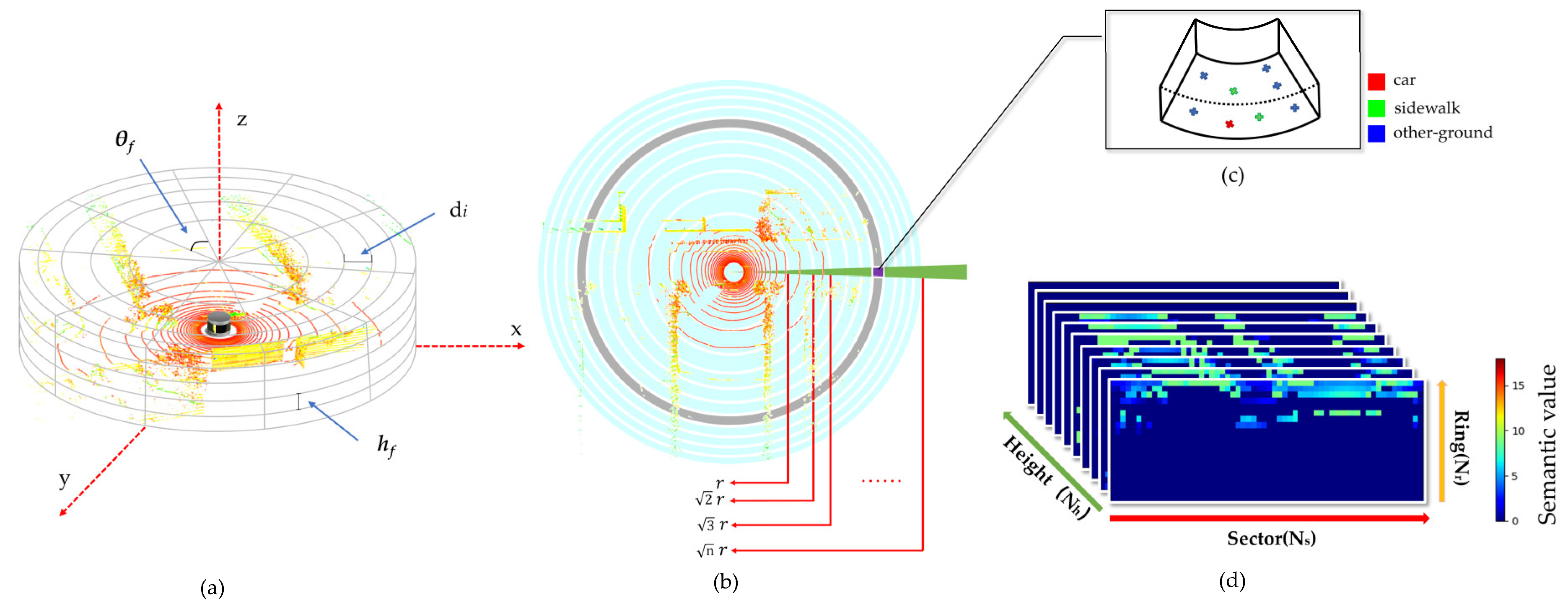
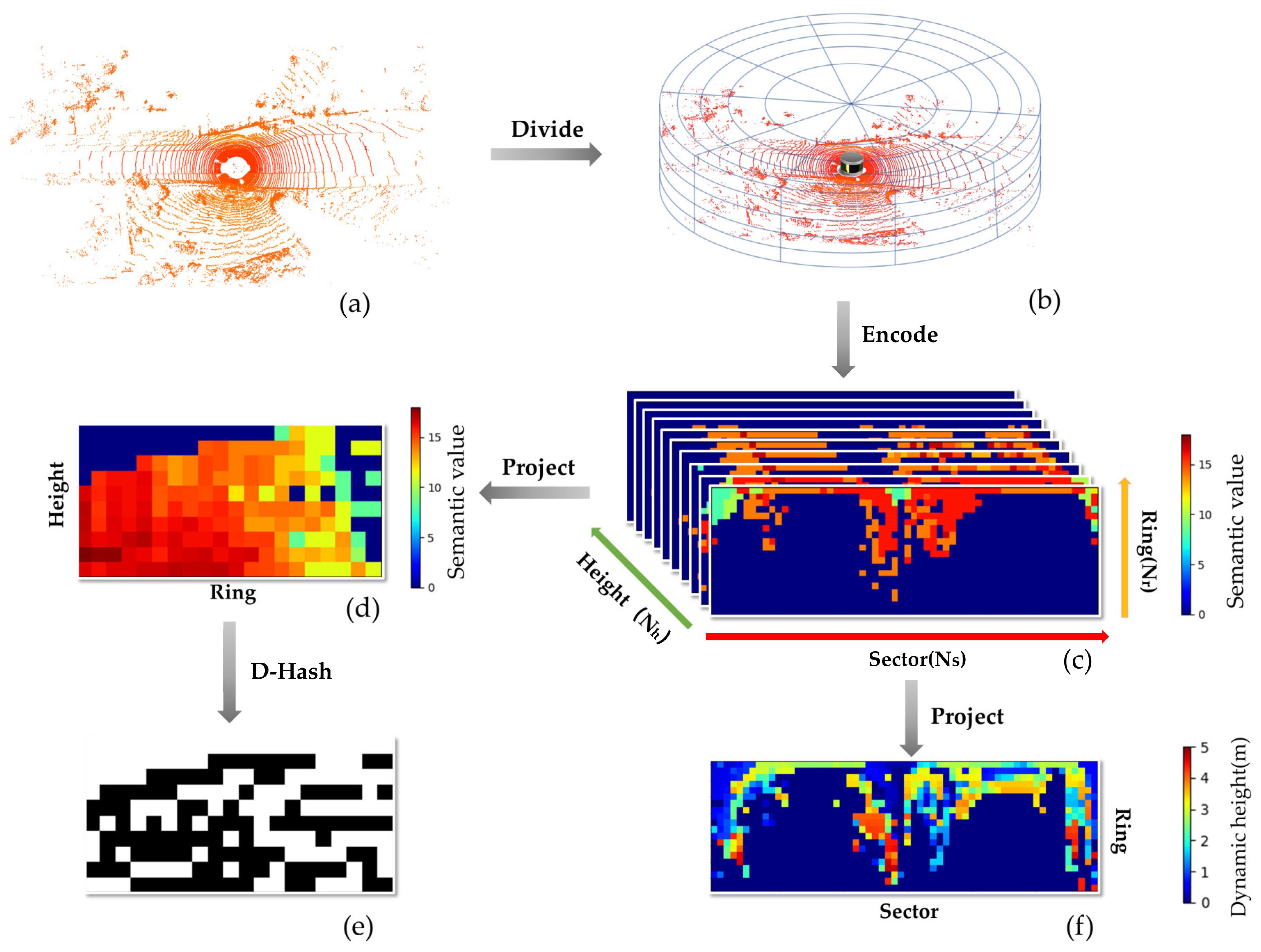
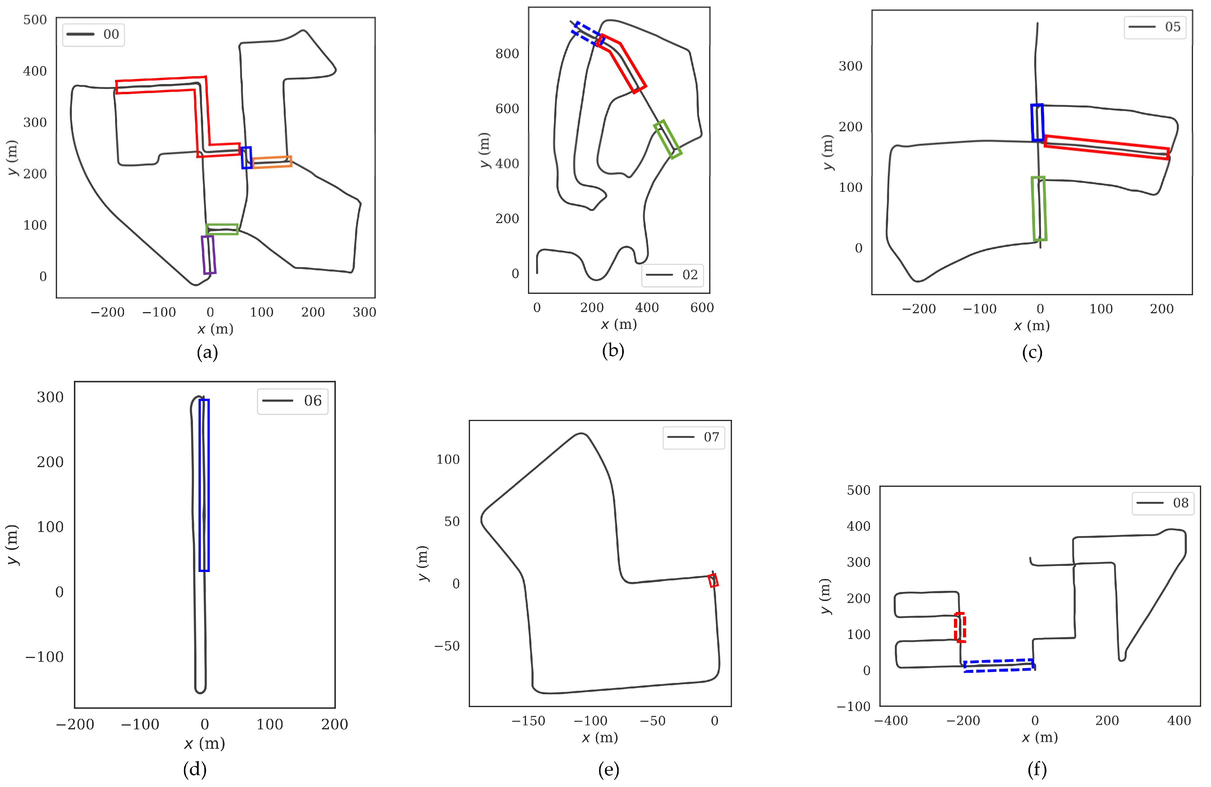
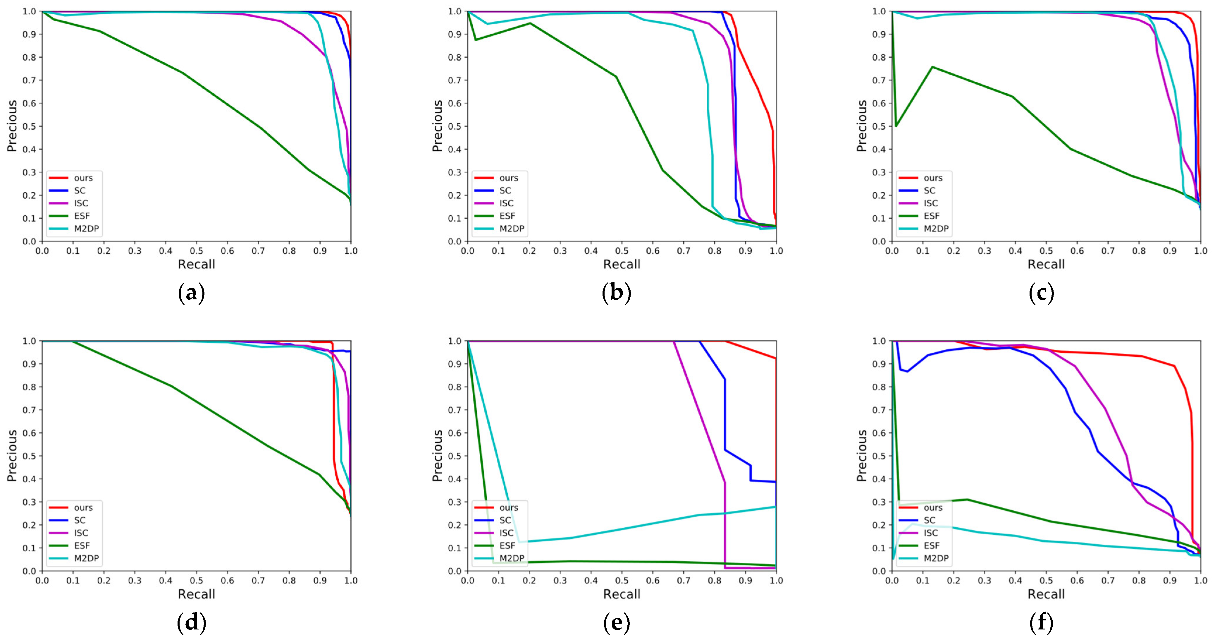
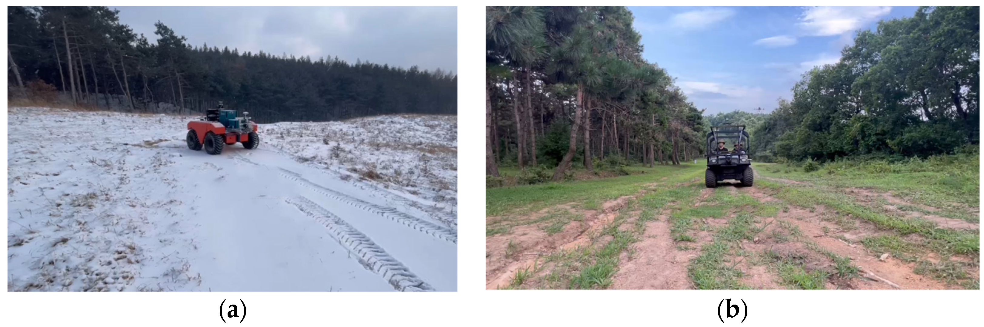
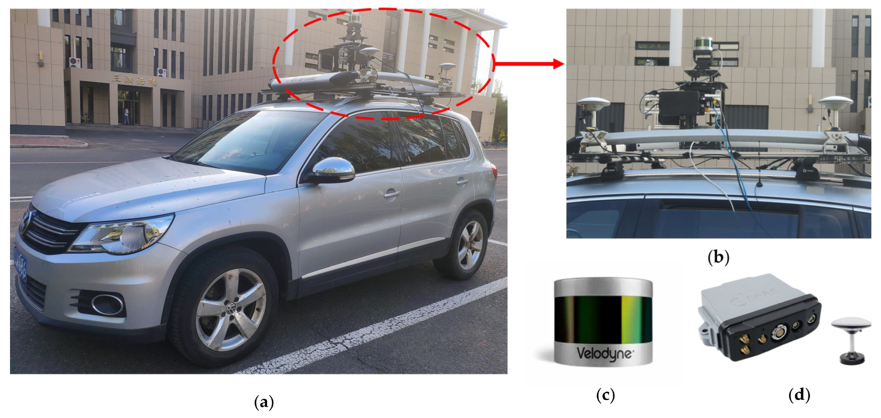
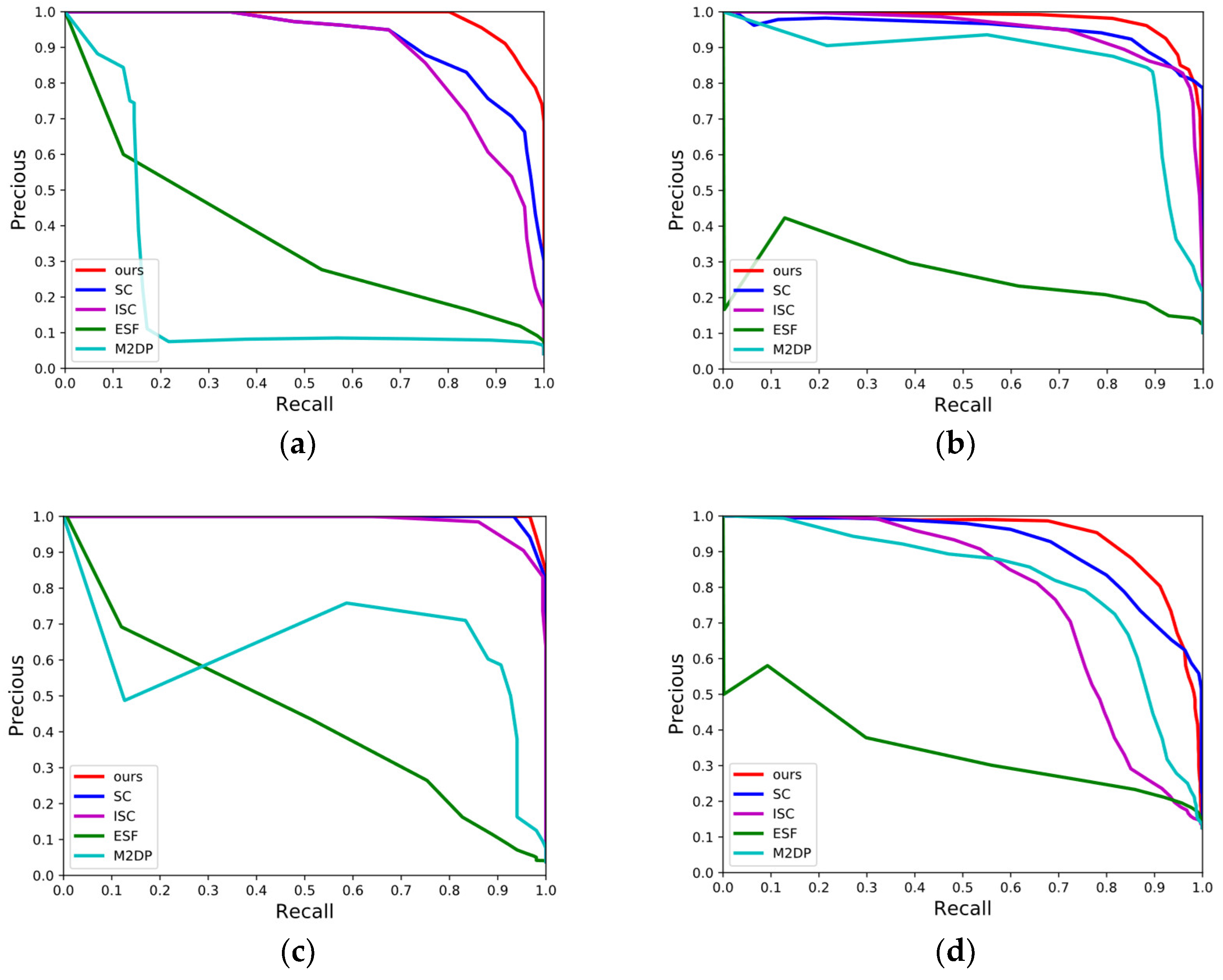
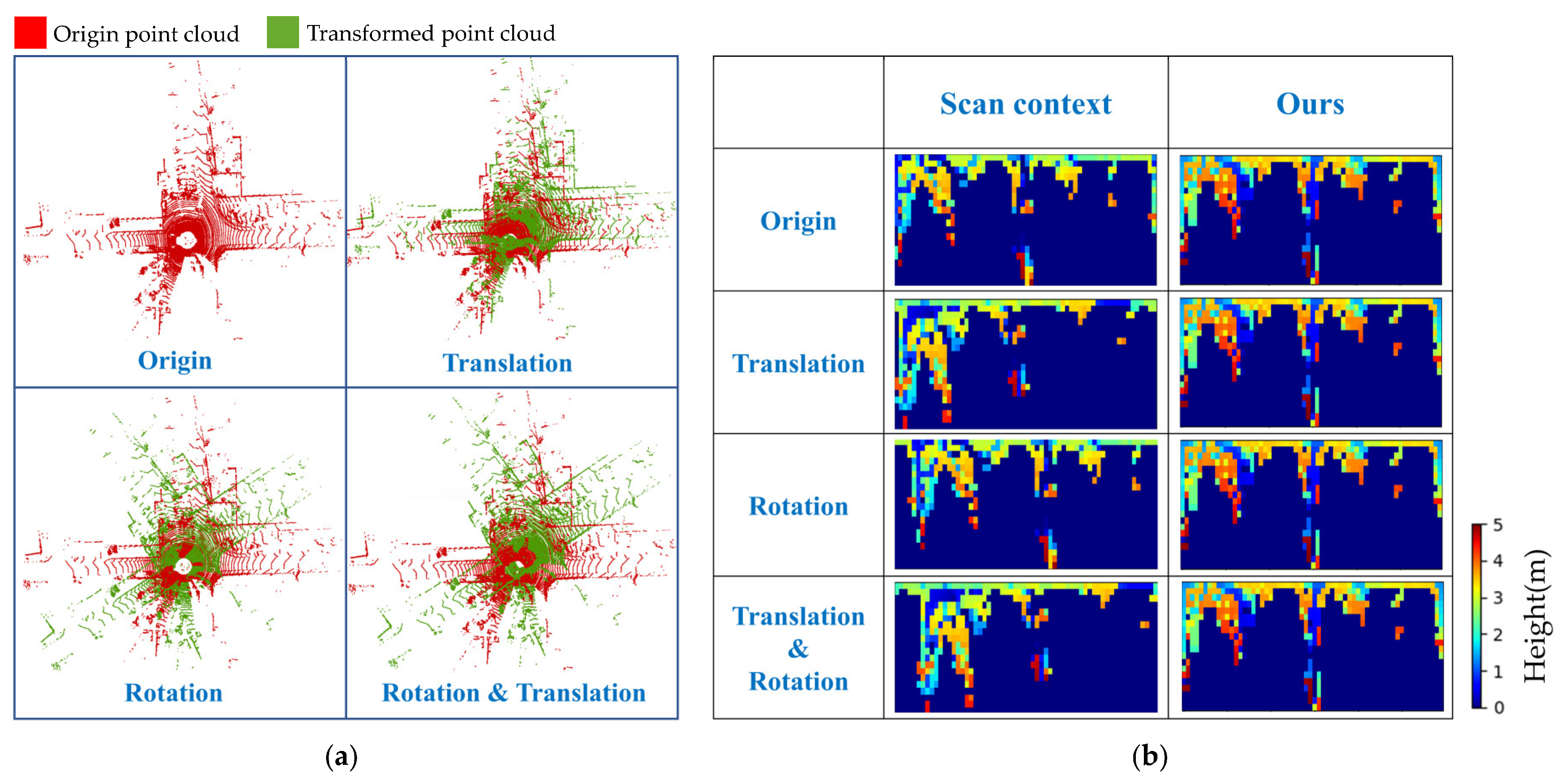
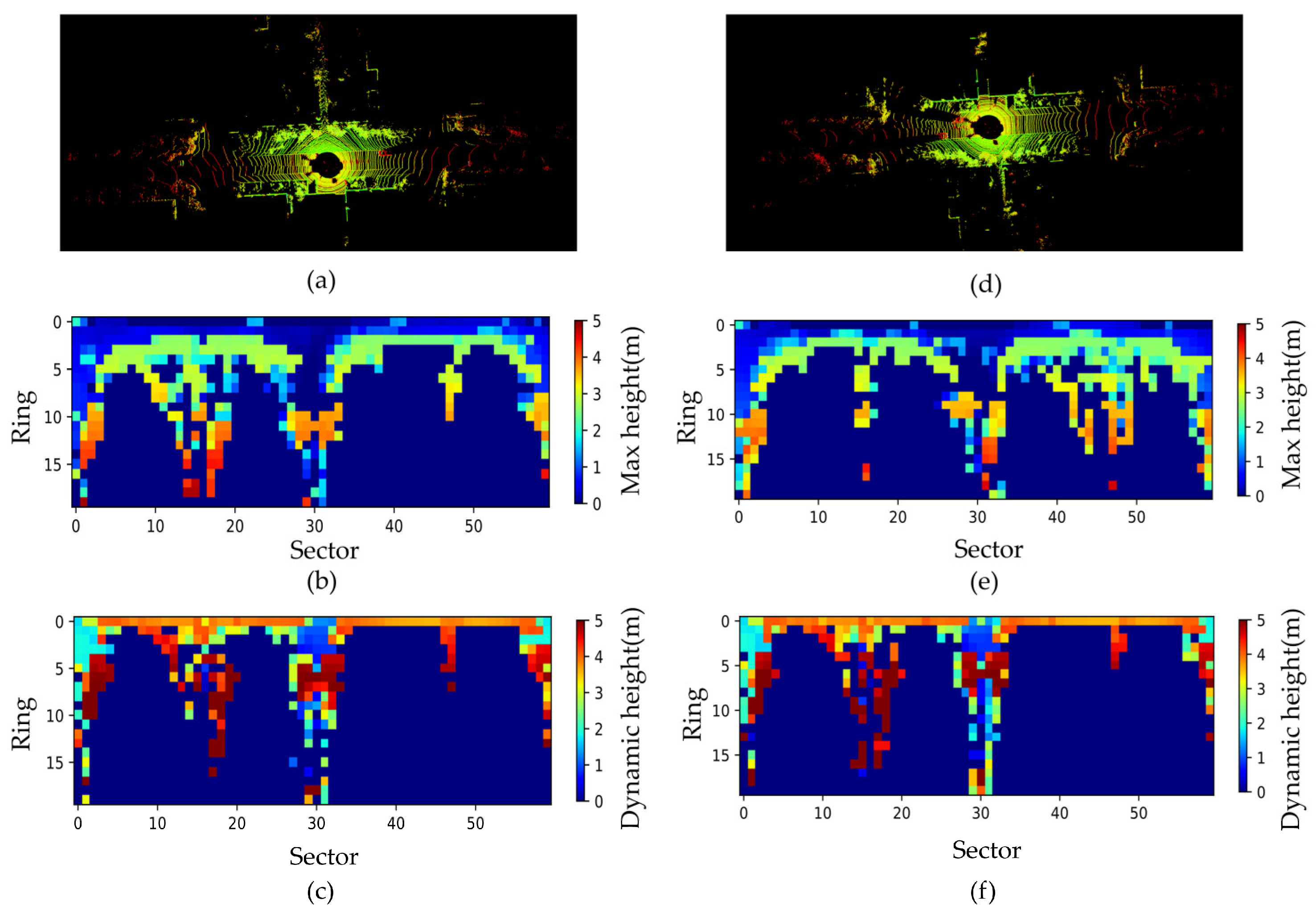
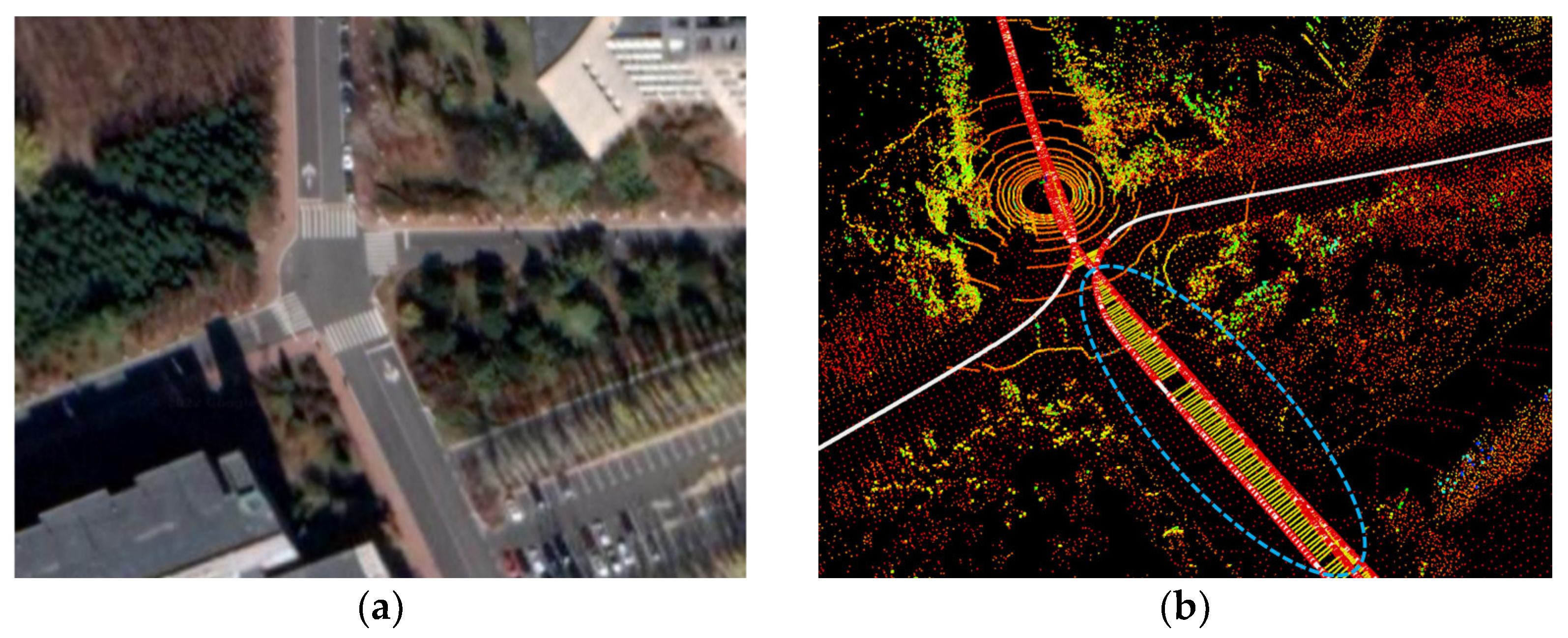
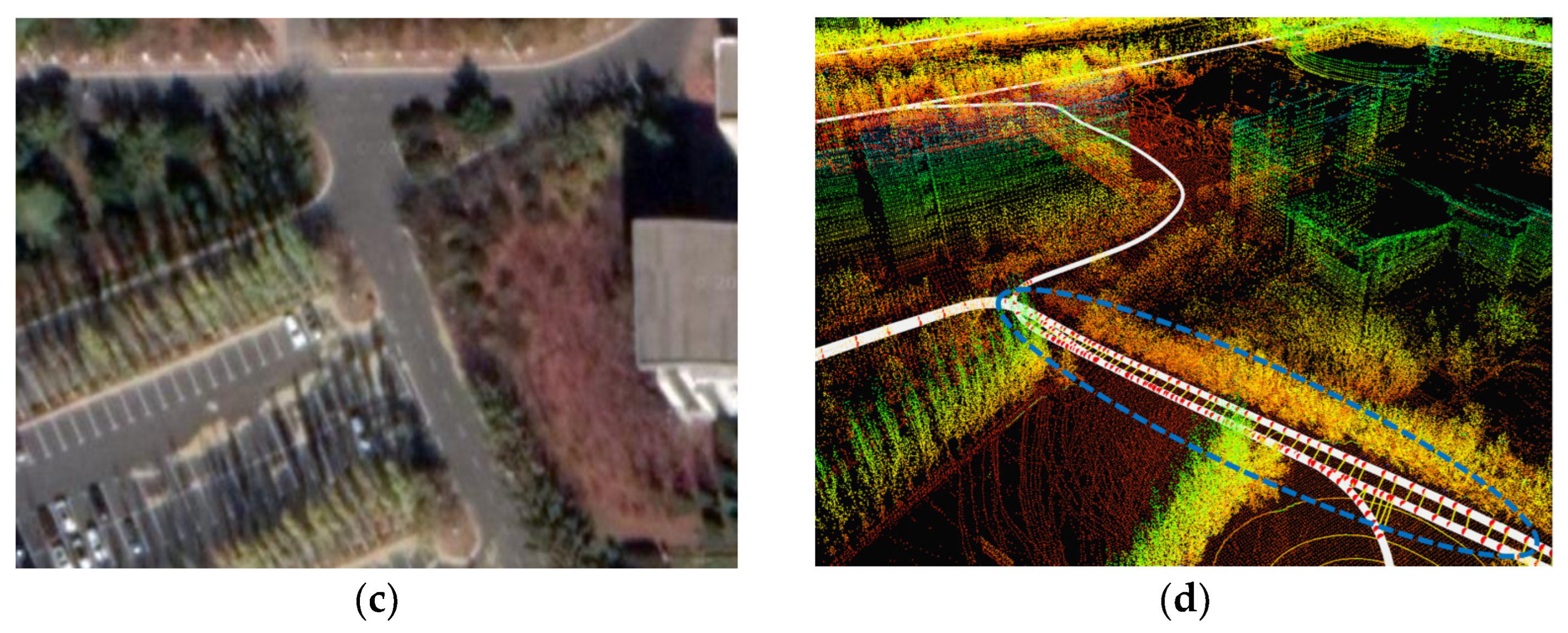
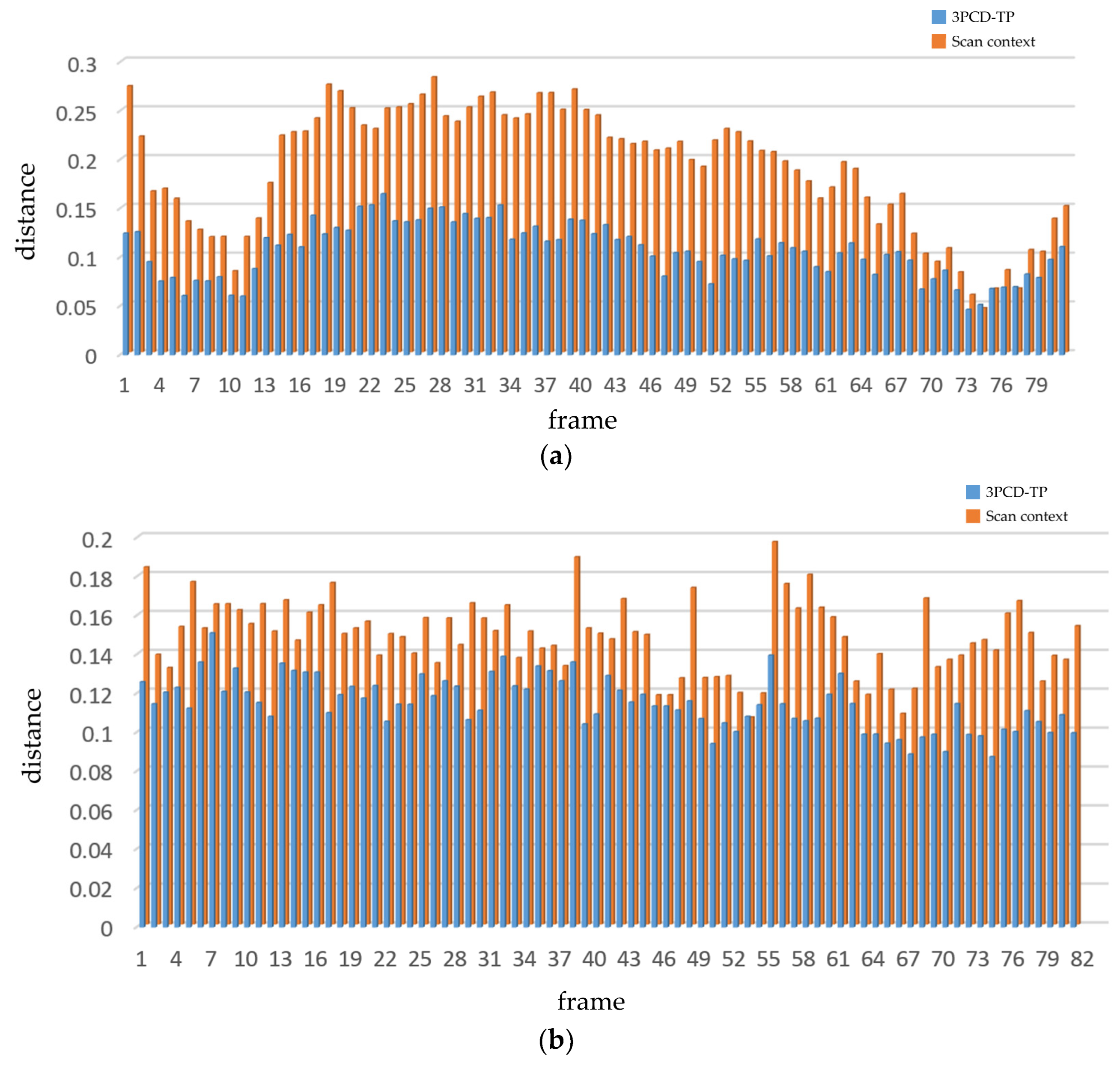
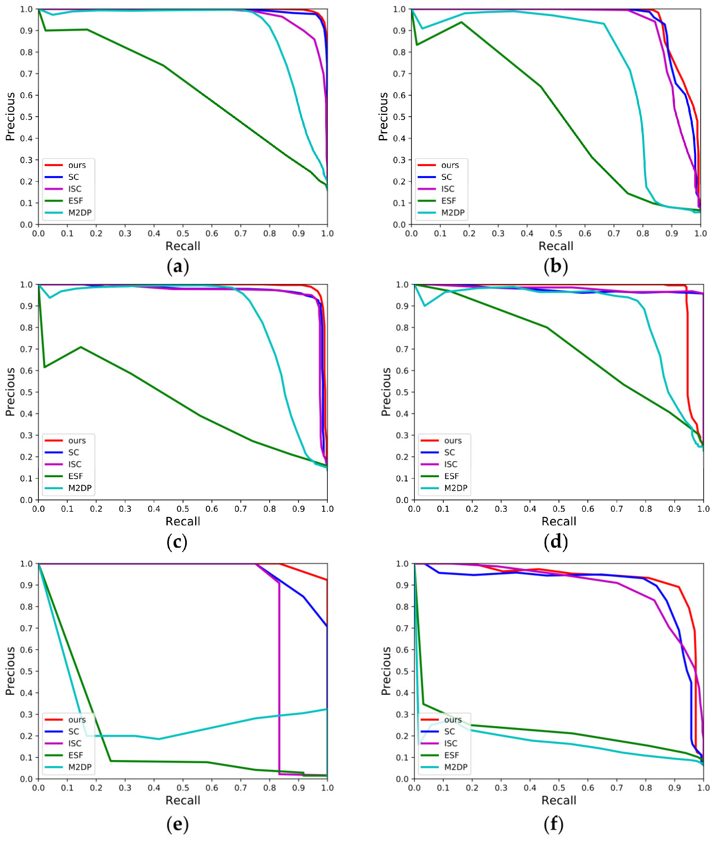
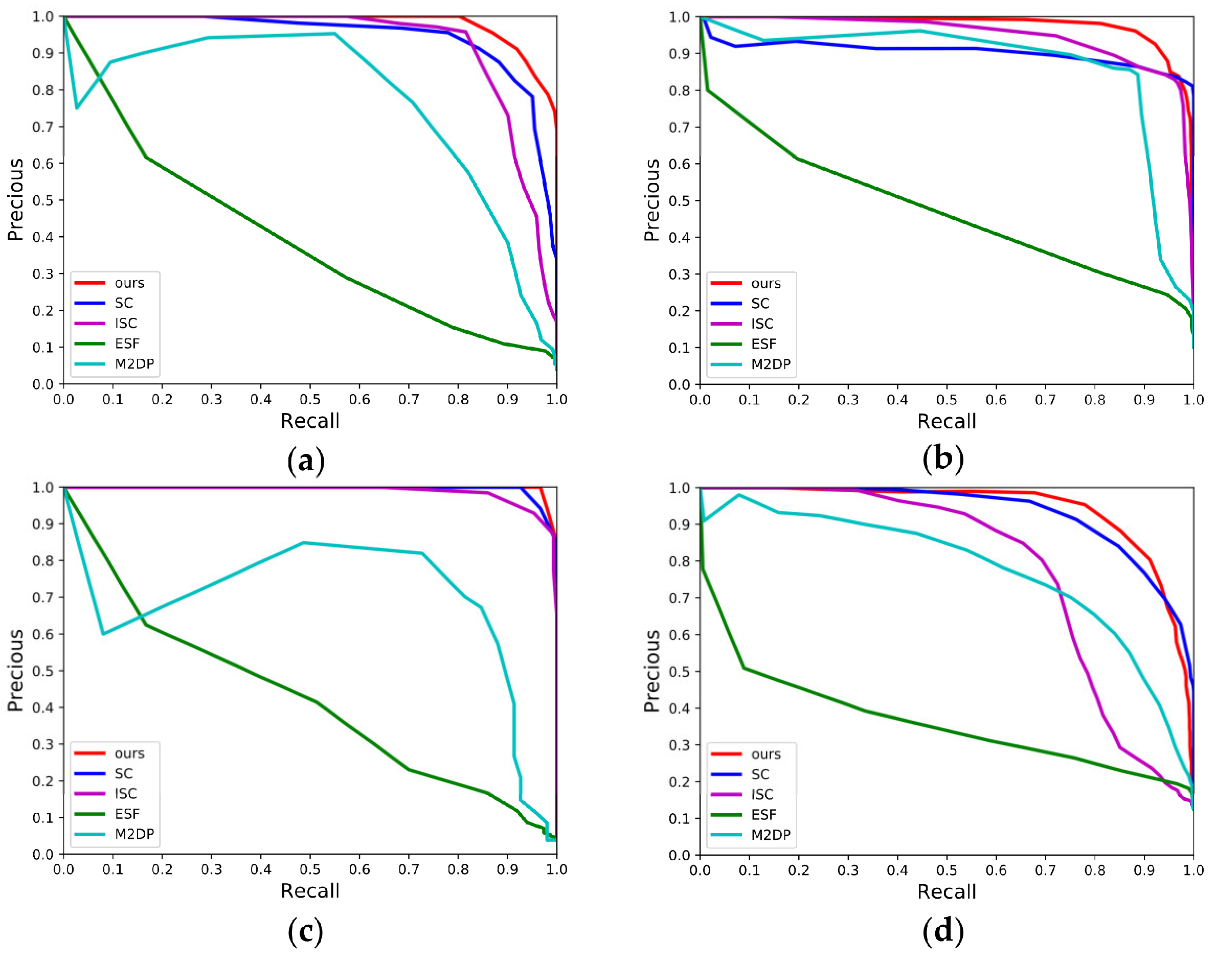
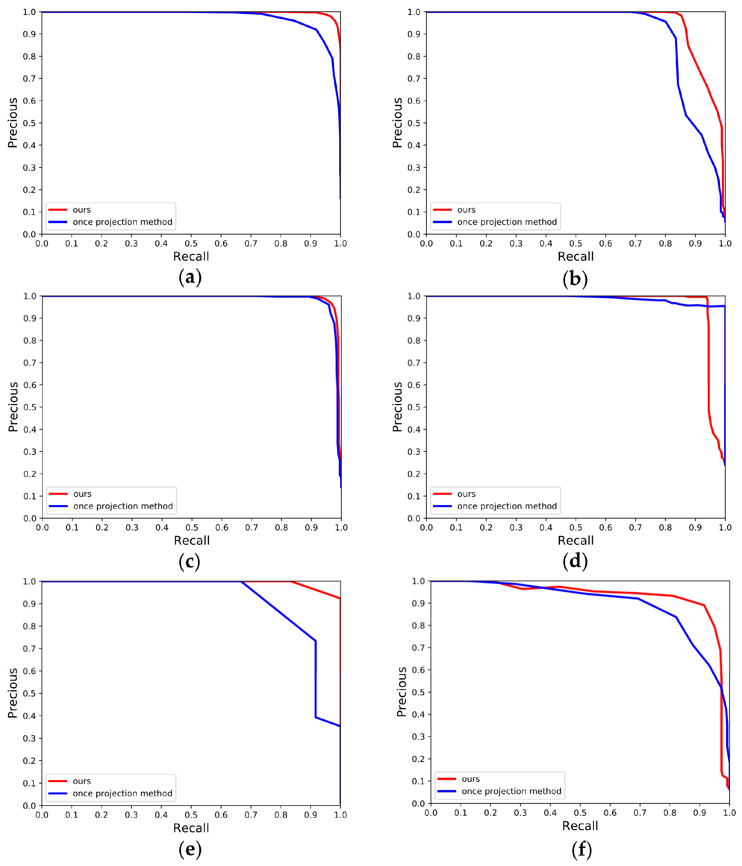
Table 1.
F1 max scores and EP on KITTI dataset.
| Methods | M2DP | ESF | SC | ISC | Ours |
|---|---|---|---|---|---|
| 00 | 0.924/0.491 | 0.580/0.482 | 0.961/0.796 | 0.870/0.638 | 0.973/0.906 |
| 02 | 0.812/0.472 | 0.575/0.438 | 0.901/0.892 | 0.857/0.703 | 0.913/0.898 |
| 05 | 0.897/0.484 | 0.481/0.250 | 0.931/0.746 | 0.883/0.647 | 0.967/0.886 |
| 06 | 0.930/0.717 | 0.623/0.547 | 0.976/0.800 | 0.941/0.812 | 0.965/0.931 |
| 07 | 0.436/0.062 | 0.075/0.017 | 0.857/0.875 | 0.800/0.833 | 0.960/0.917 |
| 08 | 0.221/0.026 | 0.303/0.143 | 0.657/0.501 | 0.712/0.614 | 0.902/0.601 |
| Avg | 0.703/0.375 | 0.440/0.313 | 0.881/0.768 | 0.843/0.709 | 0.947/0.857 |
Notes: On the left-hand side are maximum F1-scores, and on the right-hand side are EPs. The best scores are marked in bold.
Table 2.
F1 max scores and EP on School dataset.
| Methods | M2DP | ESF | SC | ISC | Ours |
|---|---|---|---|---|---|
| School-01 | 0.242/0.441 | 0.365/0.300 | 0.834/0.671 | 0.801/0.671 | 0.915/0.901 |
| School-02 | 0.963/0.453 | 0.337/0.083 | 0.890/0.513 | 0.888/0.572 | 0.924/0.613 |
| School-03 | 0.767/0.243 | 0.470/0.503 | 0.965/0.967 | 0.929/0.820 | 0.983/0.983 |
| School-04 | 0.772/0.508 | 0.391/0.250 | 0.816/0.531 | 0.727/0.602 | 0.867/0.603 |
| Avg | 0.686/0.411 | 0.391/0.284 | 0.876/0.671 | 0.836/0.666 | 0.922/0.775 |
Notes: On the left-hand side are maximum F1-scores, and on the right-hand side are Eps. The best scores are marked in bold.
Table 3.
Average execution time over KITTI dataset and JLU campus datasets.
| Methods | Avg Execution Time(s/Query) | ||||
|---|---|---|---|---|---|
| M2DP | ESF | SC | ISC | Ours | |
| KITTI-00 | 0.3655 | 0.0728 | 0.0867 | 0.0697 | 0.0711 |
| KITTI-02 | 0.3871 | 0.0784 | 0.0861 | 0.0687 | 0.0675 |
| KITTI-05 | 0.3869 | 0.0785 | 0.0885 | 0.0678 | 0.0663 |
| KITTI-06 | 0.3827 | 0.0664 | 0.0846 | 0.0656 | 0.0701 |
| KITTI-07 | 0.3451 | 0.0571 | 0.0748 | 0.0608 | 0.0631 |
| KITTI-08 | 0.3628 | 0.0751 | 0.0772 | 0.0640 | 0.0618 |
| School-01 | 0.3427 | 0.0492 | 0.0608 | 0.0530 | 0.0589 |
| School-02 | 0.3468 | 0.0552 | 0.0611 | 0.0537 | 0.0502 |
| School-03 | 0.3431 | 0.0725 | 0.0604 | 0.0533 | 0.0529 |
| School-04 | 0.3455 | 0.0732 | 0.0509 | 0.0482 | 0.0479 |
Notes: The best results are marked in bold.
Table 4.
Time comparison of different distance functions.
| Methods | Time (ms) |
|---|---|
| MAD | 0.00480 |
| SAD | 0.00488 |
| SSD | 0.00929 |
| Ours Hamming Distance | 0.000982 |
| Ours D-Hash Generation | 0.00401 |
| Ours Total | 0.00499 |
Table 5.
Time comparison of different distance functions in the actual loop closure detection.
| Methods | Avg Time (ms/Query) | |||
|---|---|---|---|---|
| MAD | SAD | SSD | Ours (D-Hash) | |
| KITTI-00 | 0.0243 | 0.0247 | 0.0467 | 0.00900 |
| KITTI-02 | 0.0241 | 0.0244 | 0.0463 | 0.00899 |
| KITTI-05 | 0.0240 | 0.0244 | 0.0464 | 0.00897 |
| KITTI-06 | 0.0240 | 0.0243 | 0.0463 | 0.00901 |
| KITTI-07 | 0.0243 | 0.0249 | 0.0468 | 0.00899 |
| KITTI-08 | 0.0239 | 0.0242 | 0.0464 | 0.00900 |
| School-01 | 0.0239 | 0.0244 | 0.0461 | 0.00897 |
| School-02 | 0.0232 | 0.0236 | 0.0467 | 0.00897 |
| School-03 | 0.0239 | 0.0241 | 0.0459 | 0.00899 |
| School-04 | 0.0242 | 0.0250 | 0.0470 | 0.00899 |
| Avg | 0.0240 | 0.0244 | 0.0465 | 0.00899 |
Notes: The best results are marked in bold.
Table 6.
F1 max scores and EP on KITTI and campus dataset.
| Methods | M2DP | ESF | SC | ISC | Ours |
|---|---|---|---|---|---|
| KITTI-00 | 0.856/0.487 | 0.570/0.450 | 0.968/0.811 | 0.908/0.810 | 0.973/0.906 |
| KITTI-02 | 0.776/0.455 | 0.527/0.417 | 0.911/0.898 | 0.889/0.729 | 0.913/0.898 |
| KITTI-05 | 0.816/0.469 | 0.460/0.308 | 0.946/0.576 | 0.948/0.623 | 0.967/0.886 |
| KITTI-06 | 0.841/0.450 | 0.615/0.484 | 0.977/0.577 | 0.976/0.524 | 0.965/0.931 |
| KITTI-07 | 0.490/0.100 | 0.137/0.042 | 0.880/0.875 | 0.870/0.875 | 0.960/0.917 |
| KITTI-08 | 0.250/0.080 | 0.305/0.174 | 0.865/0.517 | 0.829/0.562 | 0.902/0.601 |
| School-01 | 0.735/0.375 | 0.385/0.308 | 0.914/0.707 | 0.739/0.554 | 0.915/0.901 |
| School-02 | 0.864/0.468 | 0.487/0.400 | 0.897/0.503 | 0.891/0.572 | 0.924/0.613 |
| School-03 | 0.770/0.300 | 0.458/0.313 | 0.822/0.590 | 0.799/0.507 | 0.983/0.983 |
| School-04 | 0.725/0.455 | 0.406/0.389 | 0.811/0.512 | 0.744/0.604 | 0.867/0.603 |
Notes: The best results are marked in bold.
Disclaimer/Publisher’s Note: The statements, opinions and data contained in all publications are solely those of the individual author(s) and contributor(s) and not of MDPI and/or the editor(s). MDPI and/or the editor(s) disclaim responsibility for any injury to people or property resulting from any ideas, methods, instructions or products referred to in the content. |
© 2022 by the authors. Licensee MDPI, Basel, Switzerland. This article is an open access article distributed under the terms and conditions of the Creative Commons Attribution (CC BY) license (https://creativecommons.org/licenses/by/4.0/).
Share and Cite
MDPI and ACS Style
Wang, G.; Jiang, X.; Zhou, W.; Chen, Y.; Zhang, H. 3PCD-TP: A 3D Point Cloud Descriptor for Loop Closure Detection with Twice Projection. Remote Sens. 2023, 15, 82. https://doi.org/10.3390/rs15010082
AMA Style
Wang G, Jiang X, Zhou W, Chen Y, Zhang H. 3PCD-TP: A 3D Point Cloud Descriptor for Loop Closure Detection with Twice Projection. Remote Sensing. 2023; 15(1):82. https://doi.org/10.3390/rs15010082
Chicago/Turabian StyleWang, Gang, Xudong Jiang, Wei Zhou, Yu Chen, and Hao Zhang. 2023. "3PCD-TP: A 3D Point Cloud Descriptor for Loop Closure Detection with Twice Projection" Remote Sensing 15, no. 1: 82. https://doi.org/10.3390/rs15010082
Note that from the first issue of 2016, this journal uses article numbers instead of page numbers. See further details here.