Article

Inversion of Deflection of the Vertical in the South China Sea Using ICESat-2 Sea Surface Height Data

College of Geodesy and Geomatics, Shandong University of Science and Technology, Qingdao 266590, China
*
Author to whom correspondence should be addressed.
Remote Sens. 2023, 15(1), 30; https://doi.org/10.3390/rs15010030
Submission received: 12 October 2022 / Revised: 14 December 2022 / Accepted: 19 December 2022 / Published: 21 December 2022
(This article belongs to the Special Issue Ocean Observation Using Lidar)

Abstract

:
The traditional altimetry satellites based on pulse-limited radar altimeter only calculate along-track deflection of the vertical (DOV), which results in poorer precision of the prime vertical component than that of the meridian component and limits the precision of the marine gravity field inversion. We expect an improvement in the higher precision prime vertical component using the Ice, Cloud and land Elevation Satellite 2 (ICESat-2) sea surface height (SSH) data. In this paper, the 2′ × 2′ gridded DOVs derived from along-beam DOVs, cross-beam DOVs, and joint along-cross beam DOVs in the South China Sea (SCS; 0°–23°N, 103°–120°E) are calculated with the weighted least squares method, respectively. The inverse Vening–Meinesz (IVM) formula is applied to derive 2′ × 2′ gravity anomalies over the SCS from ICESat-2-derived gridded DOVs. In addition, the XGM2019e_2159-DOV and SIO V31.1-DOV models are used to assess the precision of the gridded DOVs. The XGM2019e_2159-GRA, SIO V31.1-GRA models, and ship-borne gravity anomalies are also adopted to evaluate the quality of gravity anomalies. The results show that the gridded DOVs calculated by the joint along-cross beam DOVs have the highest precision among the three gridded DOVs determined by ICESat-2. The precision of difference between gravity anomalies derived from the joint along-cross beam DOV and the above verification data are higher than those derived from the along-beam and cross-beam DOVs. We conclude that the joint along-cross beam DOV can effectively improve the precision of the gridded DOV, which is conducive to the inversion of a high-precision marine gravity field.

Graphical Abstract

1. Introduction

As important data for studying earth mass anomalies, geoid model refinement [1], and the Earth’s gravity field [2], deflection of the vertical (DOV) refers to the intersection angle between the gravitational direction of any point on the ground and the normal direction of the corresponding ellipsoid [3,4,5,6]. However, due to the existence of interference factors such as sea surface waves, currents, and tides as well as the limitation of measurement conditions, it is challenging to determine the marine DOV by conventional methods [7]. The advancement of satellite altimetry technology has fundamentally changed the defects of conventional DOV measurement methods, continuously improving the resolution and precision of marine DOV inversion [8,9,10].
At present, there are three main approaches to determine the marine DOV by using altimeter SSHs, which were proposed by Sandwell [11], Olgiati et al. [12], and Hwan, et al. [13]. Sandwell’s algorithm calculated the crossover point DOV more precisely, but the algorithm failed to invert the marine gravity field with high resolution due to the limitation of the crossover point distribution. Olgiati’s algorithm interpolates DOV perpendicular to the track direction, thus affecting the precision of DOV inversion. Hwang’s algorithm provided a method to simplify the intermediate calculation process of the gridded DOV and improve the precision of the gridded DOV. With a comprehensive comparison among the three methods, Hwang’s algorithm was adopted to invert DOV, as it is theoretically more rigorous.
Previous studies have shown that the orbital inclination of satellite altimetry affect the precision of the directional components of DOV and lead to the nonuniform precision of the prime vertical and meridian components [14,15]. Ji et al. [16] assessed the accuracy of HY-2A/GM altimeter data in estimating DOVs over the Bay of Bengal, and Wan et al. [17] verified that the standard deviations (STD) of DOV differences were 1.1″ and 3.5″ for the meridian component and the prime vertical component between HY-2A’s observations and those from EGM2008 and EIGEN-6C4 over the whole Earth’s ocean from 60°S and 60°N, respectively. They indicated that the precision of the prime vertical component was significantly poorer than that of the meridian component. In addition, most traditional altimetry satellites can only calculate the along-track DOV and are unable to calculate the cross-track DOV due to the lack of synchronous sea surface heights (SSHs) in the vertical direction of orbit. The SWOT mission provided a new approach to solving the problem of the difference in the accuracy of the directional component. Jin et al. [18] verified that DOVs determined by one cycle of SWOT data are better than the results determined by the combined dataset of Jason-1/GM, Cryosat-2/LRM, and SARAL/GM data and can significantly improve the precision of prime vertical component. In addition, the Ice, Cloud, and land Elevation Satellite 2 (ICESat-2) [19,20,21,22,23], a new generation of spaceborne lidar satellites, is expected to study the cross-beam DOV using cross-beam synchronous observations [24,25]. Moreover, the calculation of the cross-beam DOV can potentially improve the precision of the gridded DOV and make up for the shortcomings of traditional radar altimetry satellites, which can only use the along-track SSH for marine research. Compared with the traditional radar altimeter satellite, ICESat-2 satellite simultaneously transmits six beams to obtain the surface elevation information, which provides dense orbit coverage, greatly improving the orbital spacing and the spatial resolution [26]. However, ICESat-2 as a laser altimeter satellite is limited by the laser power. ICESat-2 can only provide the energy to emit three strong beams on the ocean and other low-reflective surfaces. In addition, laser observation is more susceptible to observation conditions. For rainy and cloudy weather conditions, the ICESat-2 satellite may have a large number of laser photons unable to return to the satellite, resulting in the loss of a certain section of ocean observation points.
This paper aims to use ICESat-2 SSHs measured by the multibeam photon-counting lidar system to calculate the cross-beam DOV to improve the precision of the prime vertical component. All datasets and validation models used are presented in Section 2. In Section 3, the method for calculating the meridian and prime vertical components of DOVs from ICESa-2-measured SSHs and the method for deriving gravity anomalies from DOVs are presented in detail. In Section 4, the standard deviation of crossover differences of ICESat-2 SSHs is calculated to assess the reliability of ICESat-2 SSHs. The along-beam DOV, the cross-beam DOV, and the joint along-cross beam DOV are calculated, and the corresponding 2′ × 2′ gridded DOVs are compared with the XGM2019e_2159-DOV model and SIO V31.1-DOV model. Gravity anomalies derived from gridded DOVs are evaluated by comparisons with the XG2019e_2159-GRA model, SIO V31.1-GRA model, and National Centers for Environmental Information (NCEI) ship-borne gravity anomalies.

2. Study Area and Data

2.1. Study Area

As is shown in Figure 1, the SCS (0°–23°N, 103°–120°E) was selected as the study area. Located at the southern end of mainland China, the SCS is the deepest and largest offshore area in China, which embraces the Xisha Islands, the Zhongsha Islands, the Dongsha Islands, and the Nansha Islands [27]. By virtue of its special geographical location and natural conditions, the SCS has been known as a “natural laboratory” for major scientific research such as global change and geodynamics [28].

2.2. Altimetry Data and Preprocessing

2.2.1. ICESat-2 Data

ICESat-2 was successfully launched by the National Aeronautics and Space Administration (NASA) on 15 September 2018, after the end of life of ICESat [29]. ICESat-2 uses the multibeam photon-counting lidar system to measure the height of a changing Earth [30]. ICESat-2 is equipped with the Advanced Topographic Laser Altimeter System (ATLAS), with a pulse frequency of 10 kHz, wavelength of 532 nm, orbital height of 592 km, orbital inclination of 92°, a near 91-day repeat cycle, footprint diameter of approximately 17 m, and along-beam footprint spacing of 0.7 m.
Laser pulses from ATLAS illuminate three left/right pairs of spots on the surface that, as ICESat-2 orbits Earth, trace out six ground beams. Each ground beam is numbered according to the laser spot number, with ground beam 1 L on the far left and ground beam 3R on the far right. The beams in each pair have different transmission energies, with the energy ratio between weak beams and strong beams approximating 1:4 [31,32]. Spacecraft orientation (sc_orient) determines the mapping between the strong and weak beams of ATLAS and their relative positions on the ground. Sc_orient has forward, backward, and transitional flight modes, and the value of sc_orient can judge the strong and weak orbit orientations. In the forward flight mode shown in Figure 2, the cross-beam distance between each group is approximately 3.3 km, the beam distance within the group is approximately 90 m, and the distance along the beam direction within the group is approximately 2.5 km [33].
In this paper, ATL12 with 1 Hz, the Level-3A product of ICESat-2, is processed with geophysical corrections including atmospheric delay correction, solid tide correction, sea state bias correction, ocean tide correction, pole tide correction, and inverted barometer correction. ICESat-2 SSHs can be viewed through the OpenAltimetry system (https://openaltimetry.org/data/icesat2/?product=ATL12&mapType=geographic, accessed on 1 September 2021) [34]. Its science quality is potentially degraded while in transition flight mode, and the weak-beam SSHs are sparse in pure ocean areas. Therefore, in subsequent experiments, only the strong beams in forward and backward flight modes are used.
ICESat-2 SSHs (https://doi.org/10.5067/ATLAS/ATL12.004, accessed on 1 October 2021) obtained through the National Snow and Ice Data Center (NSIDC) with the time series of 2018/10/13 to 2021/07/15 (cycle01–cycle12) are shown in Table 1. According to Table 1, the value of sc_orient determines the strong beam orientation, which helps to remove the weak beam within one cycle. The ground track of the ICESat-2 strong-beam SSHs in the SCS is shown in Figure 3a.

2.2.2. Jason-3 Data

The Jason-3 satellite [35] was jointly launched by the National Oceanic and Atmospheric Administration (NOAA), the Centre National d’Etudes Spatiales (CNES), and the European Organization for the Exploitation of Meteorological Satellites (EUMETSAT) on 17 January 2016. The Jason-3 satellite has a track height of 1336 km, track inclination of 66°, and a track period of 10 days. In this study, Jason-3/ERM SSHs with 1 Hz (https://www.ncei.noaa.gov/data/oceans/jason3/l2p, accessed on 9 October 2021) as comparison data are processed with geophysical corrections including dynamic atmospheric correction, ionospheric correction, sea state bias correction, ocean tide correction, dry troposphere and wet troposphere path delays correction, solid tide correction, pole tide correction, and inverted barometer correction. The ground track of Jason-3 SSHs with the time series of 2018/10/16 to 2021/7/13 (cycle099–cycle199) in the SCS is shown in Figure 3b.

2.3. Sea Surface Topography and Reference Gravity Field Model

The mean dynamic topography (MDT_CNES-CLS18, https://www.aviso.altimetry.fr, accessed on 12 December 2021) [36,37] with a grid resolution of 0.125° is published by AVISO. MDT_CNES-CLS18 is calculated from a combination of altimeter and space gravity data, in situ measurements, and model winds. Its input datasets include the following: the GOCO05S geoid model is used based on the complete GOCE mission and 10.5 years of GRACE data, together with all drifting buoy velocities and hydrological profiles available from 1993 to 2017.
In this paper, the Earth Gravitational Field Model 2008 (EGM2008, https://www.aviso.altimetry.fr, accessed on 12 December 2021) built by the National Geospatial-Intelligence Agency (NGA) is taken as the reference gravity field model [38] with the spherical harmonic coefficient order fully expanded to 2159, the order expanded to 2190, and a half-wavelength resolution of approximately 9 km. The model contains GRACE satellite tracking data, satellite altimeter data, and ground gravity data.

2.4. Assessment Data of DOV and Gravity Anomaly

The XGM2019e_2159-DOV model and XGM2019e_2159-GRA model (https://www.aviso.altimetry.fr, accessed on 12 December 2021) [39] are the DOV model and the gravity anomaly model obtained from XGM2019e_2159, respectively. As a combined global gravity field model, XGM2019e is represented by spheroidal harmonics up to degree and order (d/o) 5399. The model contains the satellite model GOCO06s in the longer wavelength range up to d/o 300 combined with a ground gravity grid that also covers shorter wavelengths.
The SIO V31.1-DOV model and SIO V31.1-GRA model (https://topex.ucsd.edu/pub/global_grav_1min, accessed on 26 November 2021) [40] are the global ocean DOV model and ocean gravity field mode released by the Scripps Institution of Oceanography (SIO) with a resolution of 1′ × 1′. The main improvement of SIO V31.1 with respect to SIO V30.1 is to add the latest altimetry data of Altika, Cryosat LRM, Cryosat SAR, and Sentinel-3A/B. The Altika data beginning on cycle 127, on 4 February 2019, were retracked to better accommodate the loss in amplitude associated with poor control in off-nadir pointing.
The ship-borne gravity data are commonly considered as supplementary sources of marine gravity data. With the improvement of navigation accuracy, the accuracy of marine gravity measurement by ship-borne gravimeter is also gradually improved. In addition, the measurement methods are mature, and the data processing methods are gradually improved. The ship-borne gravity data of the SCS from 1963 to 1995 (a total of 60 routes) provided by the NCEI (https://www.ncei.noaa.gov/maps/geophysics, accessed on 27 November 2021) are adopted to evaluate gravity anomalies derived from ICESat-2 SSHs. Considering the differences in observation time, observation instruments, and reference ellipsoids of each route, longwave systematic errors exist in the observations, and the EGM2008 model was selected as the reference gravity field to solve its correction parameters [41]:
Δ d g = x 0 + x 1 Δ t + x 2 Δ t 2
where Δ d g is the difference between the ship-borne gravity anomaly and the EGM2008 model; x 0 , x 1 , and x 2 are parameters to be fitted; and Δ t is the time interval.

3. Methodology

3.1. Calculation of DOV

Before the calculation of DOV, the geoid height was obtained by removing the mean dynamic topography (MDT_CNES-CLS18) from ICESat-2 SSHs. A Gaussian low-pass filter is used to filter out high-frequency errors of the geoid height to reduce the effects of sea surface variation and data noise. The response function used is as follows:
x = e d 2 2 σ 2
where d is the spherical distance between two observations, and σ is the width of the Gaussian filter. The average spherical distance between ICESat-2 SSHs’ two adjacent points along the beam direction is 3–4 km, so the filter window σ was selected as a multiple of 4 km.
The DOV is calculated by using the geoid height difference and the spherical distance at two adjacent observations [42], and the calculation formula is as follows:
ε = N q N p S
where ε is the DOV, N is the geoid height of the observation point, and S is the spherical distance between two adjacent observations along the specified direction.
A schematic diagram of the calculation method for the cross-beam DOV is shown in Figure 4, by which three strong beams can be screened out in one cycle and marked in the order from left to right: 1S, 2S, and 3S. The three strong beams are paired to form “1S_2S”, “2S_3S”, and “1S_3S”, a total of three pairs of cross-beam combinations, to calculate the cross-beam DOV, and then, “S” is divided into “L” or “R” to form six sets of cross-beam combinations. Without adding the threshold range, this will lead to a large number of calculation points of the cross-beam DOV. Therefore, this paper uses appropriate time and distance thresholds to limit the number of calculated DOVs. According to the cross-beam distance between adjacent strong beams and nonadjacent strong beams provided in Figure 2, 3.5 km and 7 km were selected as the distance thresholds for the calculation of the cross-beam DOV for adjacent strong beams and nonadjacent strong beams, respectively, with a time threshold of 1 s.
A schematic diagram of the calculation method for the joint along-cross beam DOV is shown in Figure 5, and the calculation method is similar to that for cross-beam DOV. Taking “1S_2S” as an example, the distance threshold of 3.5 km and the time threshold of 1 s were set, respectively, to calculate; there are two observation points matching point p in the cross-beam direction, namely q1 and q2. The distance threshold of 8 km along the beam direction was set. In this way, point p can be matched with one observation point along the beam and two observation points across the beam. Then, three vertical deviations can be calculated according to Equation (3). However, it is worth noting that if there is no adjacent point within 8 km along the beam direction or no cross-beam observation point satisfying the conditions in the cross-beam direction, point p will be eliminated.

3.2. Calculation of the Gridded DOV

According to the correlation between DOV and the directional components of the DOV, the relationship between DOV ε along the specified direction and its meridian component ξ and prime vertical component η is as follows:
ε = ξ cos a + η sin a
where a is the azimuth of the altimetric point along the ground track direction.
The meridian component and the prime vertical component of the gridded DOV can be directly calculated according to the DOV and azimuth at the observation point. The observation equation is as follows:
ε i + ν i = ξ ¯ cos a i + η ¯ sin a i ,   i = 1 , , n
where n is the number of observation points around the grid points to be calculated, and ν i , a i , and ε i are the residual, azimuth, and DOV along the specified direction for observation point i , respectively.
The matrix form of Equation (5) is as follows:
V = A X L
where V = ( ν 1 , , ν n ) T ; X = ( ξ ¯ η ¯ ) ; A = [ cos a 1 sin a 1 cos a n sin a n ] ; L = ( ε 1 , , ε n ) T .
Equation (6) can be solved with the indirect adjustment method:
X = ( A T P A ) 1 A T P L
P = 1 d i 2 σ i 2
where P is the weight matrix of observations, d i is the spherical distance from the observation point i to the grid point to be calculated, σ i is the standard deviation of DOV at the observation point, σ i = μ p 2 + μ q 2 S , S is the spherical distance between points p and q , and μ is the standard deviation of SSH.
Because the determinant of ( A T P A ) is close to 0, the normal equation is prone to be ill-conditioned when solving. In this paper, the ill-conditioned problem of the normal equation is solved by calculating the weighted minimum norm least squares solution; that is, the minimum norm inverse N m = ( ( A T P A ) ( A T P A ) T ) ( A T P A ) in the generalized inverse matrix is used to replace ( A T P A ) 1 to calculate the solution X of the observation equation:
X = N m A T P L

3.3. Calculation of Gravity Anomaly

Taking the calculated directional components of the gridded DOV as the input data, the inverse Vening–Meinesz formula [43] is used to invert the gravity anomaly. The directional components of the DOV at flow point q are used to calculate the gravity anomaly at fixed point p . The calculation formula is as follows:
Δ g ( p ) = γ 0 4 π σ H ( ψ ) ( ξ q cos a q p + η q sin a q p ) d σ q
where γ 0 = G M R 2 ( G M is the gravity constant, and R is the average radius of the earth); a q p is the azimuth from q to p ; ξ q and η q are the meridian and prime vertical components of DOV at point q , respectively; and H ( ψ ) , the derivative of the kernel function, can be calculated by the following formula:
H ( ψ ) = d H d ψ = cos ψ 2 2 sin 2 ψ 2 + cos ψ 2 ( 3 + 2 sin ψ 2 ) 2 sin ψ 2 ( 1 + sin ψ 2 )
where ψ is the spherical distance on the unit ball from p and q . The azimuth a q p can be calculated by the following formula:
tan a q p = cos φ p sin ( Δ λ q p ) sin ( φ q φ p ) + 2 sin φ q cos φ p sin 2 ( Δ λ q p 2 )
When calculating the gravity anomaly of grid points, the calculation point coincides with the flow point, that is, ψ = 0 , which will leave the kernel function H ( ψ ) singular and make the azimuth defy definition. Therefore, it seems necessary to calculate the influence of adding the inner zone effect on the gravity anomaly [44]. The gravity anomaly of the inner zone can be expressed as follows:
Δ g = s 0 γ 0 2 ( ξ x + η y )
s 0 = R 2 Δ λ Δ φ cos φ π
where ξ x and η y represent the change rate of the meridian and the prime vertical components of DOV in the y-axis and x-axis directions, respectively; Δ λ and Δ φ represent the longitude difference and latitude difference, respectively; and s 0 is the size of the inner circle.
The process of deriving deflection of the vertical and gravity anomalies within the SCS is visualized in Figure 6.

4. Results and Analysis

4.1. Precision Evaluation of ICESat-2 Sea Surface Height Data

This paper uses Wei Qiaoyun’s improved latitude difference method [45] to evaluate the reliability of ICESat-2 SSHs by calculating the difference in SSHs at the self-crossover points and cross-crossover points. To determine the precision of ICESat-2 SSHs, the 10-day and 91-day orbital periods and the time interval without a time limit were selected to calculate the positions of self-crossover points. The STDs of the self-crossover differences of ICESat-2 and Jason-3 are shown in Table 2. As can be seen from Table 2, the overall precision of ICESat-2 satellite is slightly lower than that of Jason-3.
As shown in Table 3, Table 4 and Table 5, according to the overall precision of ICESat-2 SSHs obtained in Table 2, the same time interval was selected to evaluate the precision of ICESat-2 single-beam SSHs. The statistical results of the self-crossover differences of ICESat-2 strong beams with different time intervals show that the precision of each strong-beam SSHs is similar, but the precision of strong-beam SSHs in the intermediate group is higher than that of the other strong beams, and the precision of “1L” and “3R” is lower than that of “3L” and “1R”, respectively.
In this paper, the difference between the cross-crossover points of two satellites is calculated by different combinations of strong beams and Jason-3 orbits. The statistical results are listed in Table 6. By analyzing the precision of the self-crossover points and cross-crossover points of two satellites, it is concluded that ICESat-2 SSHs and Jason-3 SSHs have similar centimeter precision.

4.2. Along-Beam DOV

When the corrected ICESat-2 SSHs are processed by Gaussian low-pass filtering, the appropriate filtering window should be selected because the filter process will reduce the spatial resolution of the inverse marine gravity anomaly. Gravity anomalies derived from along-beam DOV inversion under different filtering windows were compared with ship-borne gravity anomalies. The STDs of the differences are shown in Table 7. Table 7 shows that when the filtering window is chosen to be 4 km, the STD of the differences is the smallest, so a filtering window of 4 km was adopted.
The along-beam DOV is calculated by the filtered ICESat-2 SSHs and is assessed in comparison with the XGM2019e_2159-DOV model. The statistical results are shown in Table 8. Table 8 shows that the precision of the along-beam DOV of the strong beams in the intermediate group is higher than that of the other strong beams.
When calculating the gridded DOV, the data quantity and data distribution of the along-beam DOV are influenced by the size of the search radius, thus affecting the inversion precision of the gridded DOV. Table 9 shows the STD of the differences between the gridded DOV under different search radii and the SIO V31.1-DOV model. It can be concluded from Table 9 that with the expansion of the search range, the precision of the prime vertical component is gradually improved. The precision of the meridian component is the highest under a search radius of 8′. Therefore, the optimal search radius is selected as 8′.
The 2′ × 2′ gridded DOV within the SCS is derived with the weighted least squares method from along-beam DOVs, and its directional components are shown in Figure 7. The XGM2019e_2159-DOV model and SIO V31.1-DOV model are used to verify the precision of the above gridded DOV. The results are shown in Table 10 and Table 11.
Due to the design of an orbital inclination of 92°, the precision of the meridian component is higher than that of the prime vertical component. Table 10 demonstrates that the STDs of differences between the gridded DOVs calculated by six strong beams and the XGM2019e_2159-DOV model are similar. The precision of the middle strong beam is worse than that of the other two strong beams. Preliminary analysis shows that the quantity of DOV of the strong beams of the intermediate group in the search window is less and unevenly distributed, resulting in lower precision than other strong beams. The along-beam DOVs derived from the six strong beams are integrated to calculate the overall gridded DOV of all available ICESat-2 SSHs. The precision of the prime vertical component is improved significantly after ICESat-2 data integration. The variation trend of the differences in Table 11 is similar to that in Table 10.

4.3. Cross-Beam DOV

The cross-beam DOV is calculated by using the method shown in Figure 4 and is evaluated by comparisons with the XGM2019e_2159-DOV model. The statistical results are shown in Table 12. Table 12 shows that due to the uneven cutting position of the pulse emitted by ATLAS in the cutting process, the position of the strong beam of the intermediate group is slightly offset compared with that of the other strong beams. The matching degree between the strong beam of the intermediate group and other adjacent strong beams is poor. In backward mode, the precision of 1L_2L is the lowest, while in the forward mode, the precision of 2R_3R is the lowest. This verifies that the precision of single beam “1L” and “3R” is worse than that of “3L” and “1R”, respectively, in “4.1 Precision Evaluation of ICESat-2 Sea Surface Height Data”. In summary, the precision of the cross-beam DOV is approximately similar to that of the along-beam DOV, showing that the cross-beam DOV data are stable and reliable.
As shown in Figure 8, the directional components of the 2′ × 2′ gridded DOV derived from cross-beam DOVs were calculated. Then, the XGM2019e_2159-DOV model and SIO V31.1-DOV model were adopted to evaluate the precision of the derived gridded DOV. The statistical results of the differences are shown in Table 13 and Table 14.
It can be seen from Table 13 that since the azimuth angle of the cross-beam DOV is closer to the prime vertical direction than to the meridian direction, the precision of the prime vertical component of the gridded DOV is higher than that of the meridian component. Among the six different cross-beam combinations, the combination of the left strong beam and the right strong beam, namely 1L_3L and 1R_3R, has higher precision than the beam combinations containing 2L. One reason is that within the same time threshold, the azimuths of the 1L_3L and 1R_3R combinations are closer to the prime vertical direction, which results in the improvement of the precision of the prime vertical component. Second, the precision of the left strong beam is similar to that of the right strong beam, resulting in a higher precision for the combination of the left strong beam and the right strong beam. The variation trend of the differences between gridded DOVs calculated by cross-beam DOVs and the SIO V31.1-DOV model in Table 14 is similar to that in Table 13. It can be concluded that the gridded DOV derived from cross-beam DOVs is helpful to improve the precision of the prime vertical component.

4.4. Joint Along-Cross Beam DOV

To study the joint influence of the along-beam and cross-beam DOVs on the gridded DOV, the DOV data in Table 8 and Table 12 were combined. The cross-beam DOV data were added to the along-beam DOV data to form the joint along-cross beam DOV data. The XGM2019e_2159-DOV model was used to verify the precision of the combined DOV. Statistics of the differences between the joint along-cross beam DOV and the XGM2019e_2159-DOV model are shown in Table 15.
As shown in Figure 9, the directional component of the 2′ × 2′ gridded DOV is calculated by using the combined DOV. The XGM2019e_2159-DOV model and SIO V31.1-DOV model are used to evaluate the precision of the experimental results, and the statistical results are shown in Table 16 and Table 17. The results show that the precision of the meridian component of the gridded DOV calculated by the joint along-cross beam DOV is higher than that of the prime vertical component, which indicates that the joint along-cross beam DOV can effectively improve the precision of the prime vertical component.

4.5. Gravity Anomaly

The 2′ × 2′ gravity anomalies in the SCS derived from the along-beam, cross-beam, and joint along-cross beam DOVs are shown in Figure 10. The XGM2019e_2159-GRA model, SIO V31.1-GRA model, and NCEI ship-borne gravity anomalies were adopted to evaluate the quality of the gravity anomalies derived from three gridded DOVs. The difference statistics are shown in Table 18, Table 19 and Table 20. The gravity anomalies derived from the joint along-cross beam DOV were verified by the XGM2019e_2159-GRA model, SIO V31.1-GRA model, and ship-borne gravity anomaly data, achieving the highest precision of 2.49 mGal, 3.06 mGal, and 4.41 mGal, respectively. For a long time, alleviating the nonuniform precision between the meridian component and the prime vertical component of the deflection of the vertical and determining the weights of the meridional and prime vertical components for marine gravity field recovery has been key. In this paper, the gravity anomalies calculated by the joint along-cross beam DOV prove that the multi-beam synchronous observation of ICESat-2 can improve the precision of the gravity field.

5. Conclusions

In this paper, we take advantage of multibeam synchronous observations and the high spatial sampling rate of the ICESat-2 satellite to calculate the along-beam, cross-beam, and joint along-cross beam DOVs determined by ICESat-2 SSHs, and the corresponding gridded DOVs and gravity anomaly with a grid of 2′ intervals in the SCS are also calculated. The main results were summarized as follows.
(1) ICESat-2 and Jason-3/ERM SSHs have roughly the same precision, but the precision of ICESat-2 SSHs is lower than that of Jason-3/ERM SSHs.
(2) The precision of the meridian component of gridded DOV calculated by the along-beam DOV is higher than that of the prime vertical component. The azimuth angles of the cross-beam DOV are mostly biased toward the prime vertical direction, resulting in higher precision of the prime vertical component than that of the meridian component. The meridian and prime vertical components calculated by the joint along-cross beam DOV are verified by XGM2019e_2159-DOV model with the precision of 0.84″ and 1.55″, respectively, and they are verified by SIO V31.1_DOV model with the precision of 0.80″ and 1.51″, respectively. It can be concluded that the joint along-cross beam DOV can effectively improve the precision of the gridded DOV and reduce the precision difference between the prime vertical component and meridian component of the gridded DOV.
(3) The STDs of differences between gravity anomalies derived from the joint along-cross beam DOVs and XGM2019e_2159-GRA model, SIO V31.1-GRA model, and the ship-borne gravity anomalies are 2.49 mGal, 3.06 mGal, and 4.41 mGal, respectively, which are higher than those derived from along-beam and cross-beam DOVs. Compared with the traditional radar altimeter satellites, the precision of gravity anomaly derived from ICESat-2 is not significantly improved. In addition to the precision and density of sea surface height data, the gravity anomaly is also affected by other environmental factors, including the coastline, water depth, and seabed terrain changes, which are also the key to the study of marine gravity anomalies. ICESat-2 SSH data still show much room for improvement in gravity field inversion.
Establishing a gravity anomaly model derived from multi-satellites altimeter data is a major trend in marine research, which means that the technical method in this paper still needs to be further improved. How to integrate altimeter data with different observation frequencies and different survey missions to establish a high-precision and high-resolution marine gravity anomaly model is a problem that needs to be considered in the next step.

Author Contributions

Conceptualization, X.L. and G.H.; methodology, X.L., G.H. and J.G.; software, T.Z. and M.S.; validation, X.L., G.H. and J.G.; formal analysis, X.L.; investigation, X.L. and T.Z.; resources, J.G.; data curation, X.L. and G.H.; writing—original draft, X.L.; writing—review and editing, J.G.; visualization, G.H. and M.S.; supervision, J.G.; project administration, X.L.; funding acquisition, X.L. and J.G. All authors have read and agreed to the published version of the manuscript.
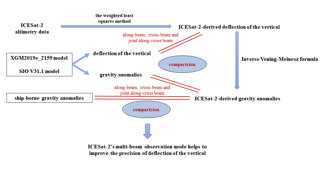
Funding

This research was funded by the National Natural Science Foundation of China, grant number 42274006; the Autonomous and Controllable Special Project for Surveying and Mapping of China, grant number 816-517; and the SDUST Research Fund, grant number 2014TDJH101.

Data Availability Statement

The multi-source data of feature extracted in this study is available at the following address: ICESat-2 data: https://doi.org/10.5067/ATLAS/ATL12.004 (accessed on 1 October 2021); Jason-3 data: https://www.ncei.noaa.gov/data/oceans/jason3/l2p (accessed on 9 October 2021); NCEI ship-borne gravity data: https://www.ncei.noaa.gov/maps/geophysics (accessed on 27 November 2021); the mean dynamic topography model: https://www.aviso.altimetry.fr (accessed on 12 December 2021); XGM2019e_2159-DOV model and XGM2019e_2159-GRA model: https://topex.ucsd.edu/pub/global_grav_1min (accessed on 12 December 2021); SIO V31.1-DOV model and SIO V31.1-GRA model: http://icgem.gfz-potsdam.de/calcgrid (accessed on 26 November 2021).

Conflicts of Interest

The authors declare no conflict of interest.

References

  1. Featherstone, W.E.; Olliver, J.G. Assessment of EGM2008 over Britain using vertical deflections, and problems with historical data. Surv. Rev. 2013, 45, 319–324. [Google Scholar] [CrossRef] [Green Version]
  2. Zhang, S.; Sandwell, D.T.; Jin, T.; Li, D. Inversion of marine gravity anomalies over southeastern China seas from multi-satellite altimeter vertical deflections. J. Appl. Geophys. 2017, 137, 128–137. [Google Scholar] [CrossRef] [Green Version]
  3. Guo, J.; Shen, Y.; Zhang, K.; Liu, X.; Kong, Q.; Xie, F. Temporal-spatial distribution of oceanic vertical deflections determined by TOPEX/Poseidon and Jason-1/2 missions. Earth Sci. Res. J. 2016, 20, h1–h5. [Google Scholar] [CrossRef] [Green Version]
  4. Liu, Q.; Xu, K.; Jiang, M. A new DOV gridding method and its application in marine gravity recovery. IEEE Geosci. Remote Sens. Lett. 2022, 19, 8025205. [Google Scholar] [CrossRef]
  5. Nguyen, V.-S.; Pham, V.-T.; Nguyen, L.V.; Andersen, O.B.; Forsberg, R.; Bui, D.T. Marine gravity anomaly mapping for the Gulf of Tonkin area (Vietnam) using Cryosat-2 and Saral/AltiKa satellite altimetry data. Adv. Space Res. 2020, 66, 505–519. [Google Scholar] [CrossRef]
  6. Boyarsky, E.A.; Afanasyeva, L.V.; Koneshov, V.N.; Rozhkov, Y.E. On calculation of the vertical deflection and the geoid undulation from gravity anomalies. Izv. Phys. Solid Earth 2010, 46, 538–543. [Google Scholar] [CrossRef]
  7. Guo, J.; Liu, X.; Chen, Y.; Wang, J.; Li, C. Local normal height connection across sea with ship-borne gravimetry and GNSS techniques. Mar. Geophys. Res. 2014, 35, 141–148. [Google Scholar] [CrossRef]
  8. Liu, S.; Li, Y.; Sun, Q.; Wan, J.; Jiao, Y.; Jiang, J. Evaluation of marine gravity anomaly calculation accuracy by multi-source satellite altimetry data. Front. Earth Sci. 2021, 9, 730777. [Google Scholar] [CrossRef]
  9. Ji, H.; Liu, X.; Zhu, C.; Yuan, J.; Ji, B.; Guo, J. On performance of CryoSat-2 altimeter data in deriving marine gravity over the Bay of Bengal. Mar. Geophys. Res. 2021, 42, 39. [Google Scholar] [CrossRef]
  10. Zhu, C.; Guo, J.; Gao, J.; Liu, X.; Hwang, C.; Yu, S.; Yuan, J.; Ji, B.; Guan, B. Marine gravity determined from multi-satellite GM/ERM altimeter data over the South China Sea: SCSGA V1.0. J. Geod. 2020, 94, 50. [Google Scholar] [CrossRef]
  11. Sandwell, D.T. Antarctic marine gravity field from high-density satellite altimetry. Geophys. J. Int. 1992, 109, 437–448. [Google Scholar] [CrossRef] [Green Version]
  12. Olgiati, A.; Balmino, G.; Sarrailh, M. Gravity anomalies from satellite altimetry: Comparison between computation via geoid heights and via deflections of the vertica. Bull. Géodésique 1995, 69, 252–260. [Google Scholar] [CrossRef]
  13. Hwang, C.; Kao, E.-C.; Parsons, B. Global derivation of marine gravity anomalies from Seasat, Geosat, ERS-1 and TOPEX/POSEIDON altimeter data. Geophys. J. Int. 1998, 134, 449–459. [Google Scholar] [CrossRef] [Green Version]
  14. Che, D.; Li, H.; Zhang, S.; Ma, B. Calculation of deflection of vertical and gravity anomalies over the South China Sea derived from ICESat-2 data. Front. Earth Sci. 2021, 9, 670256. [Google Scholar] [CrossRef]
  15. Wan, X.; Jin, S.; Liu, B.; Tian, S.; Kong, W.; Annan, R.F. Effects of interferometric radar altimeter errors on marine gravity field inversion. Sensors 2020, 20, 2465. [Google Scholar] [CrossRef]
  16. Ji, H.; Guo, J.; Zhu, C.; Yuan, J.; Liu, X.; Li, G. On deflections of vertical determined from HY-2A/GM altimetry data in the Bay of Bengal. IEEE J. Sel. Top. Appl. Earth Obs. Remote Sens. 2021, 14, 12048–12060. [Google Scholar] [CrossRef]
  17. Wan, X.; Annan, R.F.; Jin, S.; Gong, X. Vertical deflections and gravity disturbances derived from HY-2A data. Remote Sens. 2020, 12, 2287. [Google Scholar] [CrossRef]
  18. Jin, T.; Zhou, M.; Zhang, H.; Li, J.; Jiang, W.; Zhang, S.; Hu, M. Analysis of vertical deflections determined from one cycle of simulated SWOT wide-swath altimeter data. J. Geod. 2022, 96, 30. [Google Scholar] [CrossRef]
  19. Abdalati, W.; Zwally, H.J.; Bindschadler, R.; Csatho, B.; Farrell, S.L.; Fricker, H.A.; Harding, D.; Kwok, R.; Lefsky, M.; Markus, T.; et al. The ICESat-2 laser altimetry mission. Proc. IEEE 2010, 98, 735–751. [Google Scholar] [CrossRef]
  20. Magruder, L.; Neumann, T.; Kurtz, N. ICESat-2 early mission synopsis and observatory performance. Earth Space Sci. 2021, 8, e2020EA001555. [Google Scholar] [CrossRef]
  21. Magruder, L.A.; Brunt, K.M. Performance analysis of airborne photon-counting lidar data in preparation for the ICESat-2 mission. IEEE Trans. Geosci. Remote Sens. 2018, 56, 2911–2918. [Google Scholar] [CrossRef]
  22. Morison, J.H.; Hancock, D.; Dickinson, S.; Robbins, J.; Roberts, L.; Kwok, R.; Palm, S.P.; Smith, B.; Jasinski, M.F.; The ICESat-2 Science Team. ATLAS/ICESat-2 L3A Ocean Surface Height, Version 4; NASA National Snow and Ice Data Center Distributed Active Archive Center: Boulder, CO, USA, 2021. [Google Scholar] [CrossRef]
  23. Markus, T.; Neumann, T.; Martino, A.; Abdalati, W.; Brunt, K.; Csatho, B.; Farrell, S.; Fricker, H.; Gardner, A.; Harding, D.; et al. The Ice, Cloud, and land Elevation Satellite-2 (ICESat-2): Science requirements, concept, and implementation. Remote Sens. Environ. 2017, 190, 260–273. [Google Scholar] [CrossRef]
  24. Luthcke, S.B.; Thomas, T.C.; Pennington, T.A.; Rebold, T.W.; Nicholas, J.B.; Rowlands, D.D.; Gardner, A.S.; Bae, S. ICESat-2 pointing calibration and geolocation performance. Earth Space Sci. 2021, 8, e2020EA001494. [Google Scholar] [CrossRef]
  25. Yu, Y.; Sandwell, D.T.; Gille, S.T.; Villas Bôas, A.B. Assessment of ICESat-2 for the recovery of ocean topography. Geophys. J. Int. 2021, 226, 456–467. [Google Scholar] [CrossRef]
  26. Li, Z.; Guo, J.; Ji, B.; Wan, X.; Zhang, S. A Review of Marine Gravity Field Recovery from Satellite Altimetry. Remote Sens. 2022, 14, 4790. [Google Scholar] [CrossRef]
  27. Zhu, C.; Guo, J.; Hwang, C.; Gao, J.; Yuan, J.; Liu, X. How HY-2A/GM altimeter performs in marine gravity derivation: Assessment in the South China Sea. Geophys. J. Int. 2019, 219, 1056–1064. [Google Scholar] [CrossRef]
  28. Morton, B.; Blackmore, G. South China Sea. Mar. Pollut. Bull. 2001, 42, 1236–1263. [Google Scholar] [CrossRef]
  29. Xu, Y.; Li, H.; Liu, B.; Xie, H.; Ozsoy-Cicek, B. Deriving antarctic sea-ice thickness from satellite altimetry and estimating consistency for NASA’s ICESat/ICESat-2 missions. Geophys. Res. Lett. 2021, 48, e2021GL093425. [Google Scholar] [CrossRef]
  30. Neumann, T.A.; Martino, A.J.; Markus, T.; Bae, S.; Bock, M.R.; Brenner, A.C.; Brunt, K.M.; Cavanaugh, J.; Fernandes, S.T.; Hancock, D.W.; et al. The Ice, Cloud, and Land Elevation Satellite-2 mission: A global geolocated photon product derived from the Advanced Topographic Laser Altimeter System. Remote Sens. Environ. 2019, 233, 111325. [Google Scholar] [CrossRef]
  31. Zhu, X.; Nie, S.; Wang, C.; Xi, X. The performance of ICESat-2’s strong and weak beams in estimating ground elevation and forest height. In Proceedings of the IEEE International Geoscience and Remote Sensing Symposium, Waikoloa, HI, USA, 26 September–2 October 2020; pp. 6073–6076. [Google Scholar] [CrossRef]
  32. Michaelides, R.J.; Bryant, M.B.; Siegfried, M.R.; Borsa, A.A. Quantifying surface-height change over a periglacial environment with ICESat-2 laser altimetry. Earth Space Sci. 2021, 8, e2020EA001538. [Google Scholar] [CrossRef]
  33. Lu, X.; Hu, Y.; Yang, Y. Ocean subsurface study from ICESat-2 mission. In Proceedings of the Photonics and Electromagnetics Research Symposium—Fall (PIERS—Fall), Xiamen, China, 17–20 December 2019; pp. 910–918. [Google Scholar] [CrossRef]
  34. Khalsa, S.J.S.; Borsa, A.; Nandigam, V.; Phan, M.; Lin, K.; Crosby, C.; Fricker, H.; Baru, C.; Lopez, L. OpenAltimetry—Rapid analysis and visualization of Spaceborne altimeter data. Earth Sci. Inform. 2022, 15, 1471–1480. [Google Scholar] [CrossRef] [PubMed]
  35. Maiwald, F.; Montes, O.; Padmanabhan, S.; Michaels, D.; Kitiyakara, A.; Jarnot, R.; Brown, S.T.; Dawson, D.; Wu, A.; Hatch, W.; et al. Reliable and stable radiometers for Jason-3. IEEE J. Sel. Top. Appl. Earth Obs. Remote Sens. 2016, 9, 2754–2762. [Google Scholar] [CrossRef]
  36. Becker, S.; Brockmann, J.M.; Schuh, W.D. Mean dynamic topography estimates purely based on GOCE gravity field models and altimetry. Geophys. Res. Lett. 2014, 41, 2063–2069. [Google Scholar] [CrossRef]
  37. Mulet, S.; Rio, M.-H.; Etienne, H.; Artana, C.; Cancet, M.; Dibarboure, G.; Feng, H.; Husson, R.; Picot, N.; Provost, C.; et al. The new CNES-CLS18 global mean dynamic topography. Ocean. Sci. 2021, 17, 789–808. [Google Scholar] [CrossRef]
  38. Pavlis, N.K.; Holmes, S.A.; Kenyon, S.C.; Factor, J.K. The development and evaluation of the Earth Gravitational Model 2008 (EGM2008). J. Geophys. Res. Solid Earth 2012, 117, 008916. [Google Scholar] [CrossRef] [Green Version]
  39. Zingerle, P.; Pail, R.; Gruber, T.; Oikonomidou, X. The combined global gravity field model XGM2019e. J. Geod. 2020, 94, 66. [Google Scholar] [CrossRef]
  40. Sandwell, D.T.; Harper, H.; Tozer, B.; Smith, W.H.F. Gravity field recovery from geodetic altimeter missions. Adv. Space Res. 2021, 68, 1059–1072. [Google Scholar] [CrossRef]
  41. Hwang, C.; Parsons, B. Gravity anomalies derived from Seasat, Geosat, ERS-1 and TOPEX/POSEIDON altimetry and ship gravity: A case study over the Reykjanes Ridge. Geophys. J. Int. 1995, 122, 551–568. [Google Scholar] [CrossRef]
  42. Zhang, S.; Andersen, O.B.; Kong, X.; Li, H. Inversion and validation of improved marine gravity field recovery in South China Sea by incorporating HY-2A altimeter waveform data. Remote Sens. 2020, 12, 802. [Google Scholar] [CrossRef] [Green Version]
  43. Yu, D.; Hwang, C.; Andersen, O.B.; Chang, E.T.Y.; Gaultier, L. Gravity recovery from SWOT altimetry using geoid height and geoid gradient. Remote Sens. Environ. 2021, 265, 112650. [Google Scholar] [CrossRef]
  44. Zhu, C.; Guo, J.; Yuan, J.; Li, Z.; Liu, X.; Gao, J. SDUST2021GRA: Global marine gravity anomaly model recovered from Ka-band and Ku-band satellite altimeter data. Earth Syst. Sci. Data 2022, 14, 4589–4606. [Google Scholar] [CrossRef]
  45. Wei, Q.Y. A Method for Location Determination of Intersections and Related Data Processing. Master’s Thesis, Henan University, Henan, China, 2017. [Google Scholar]
Figure 1. Topographic map of the South China Sea.
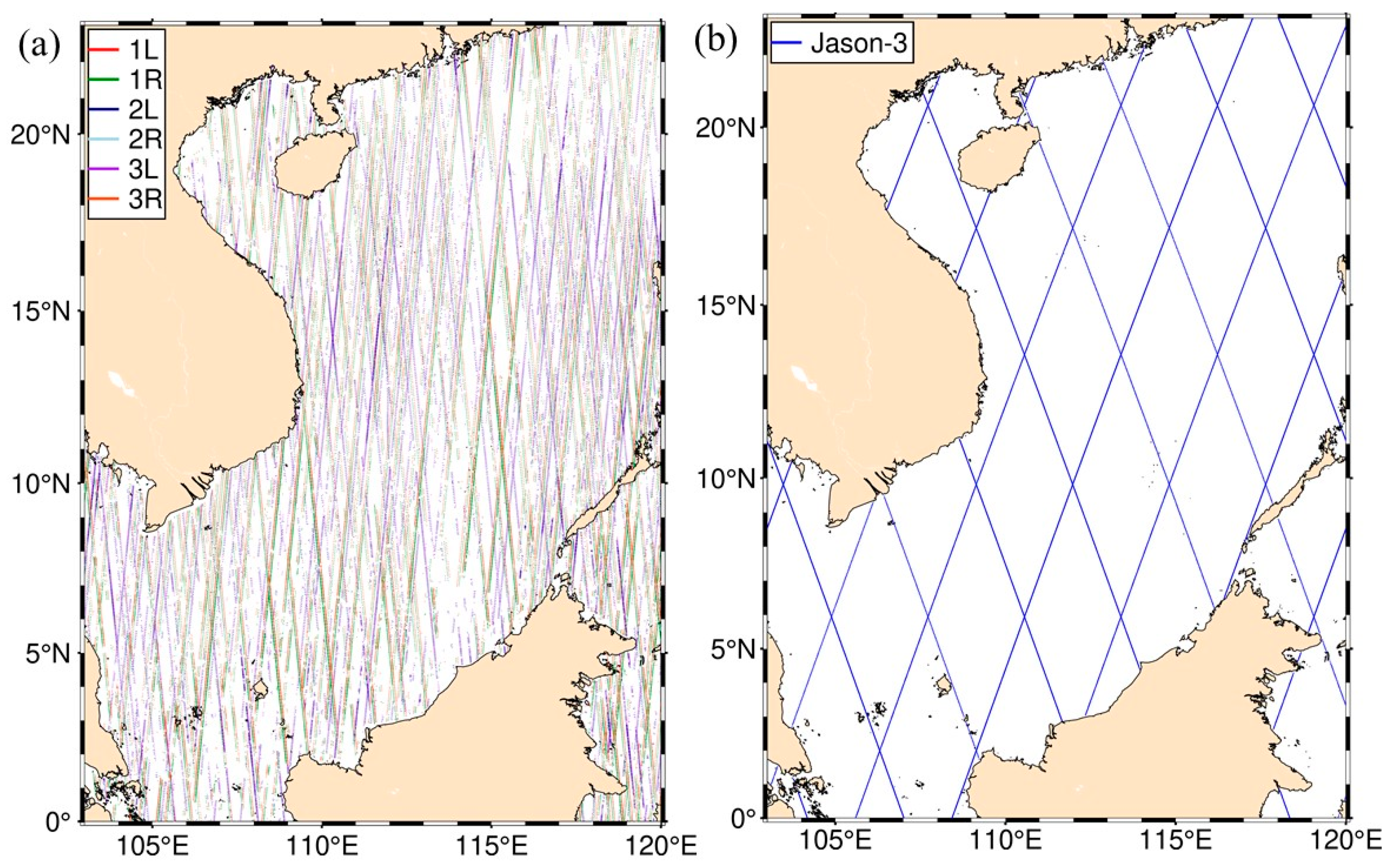
Remotesensing 15 00030 g001
Figure 2. Beam distribution of ATLAS under the forward flight mode (+x direction) (https://icesat-2.gsfc.nasa.gov (accessed on 2 January 2021)).
Remotesensing 15 00030 g002
Figure 3. (a) Ground track of ICESat-2 strong-beam SSHs in the SCS; (b) ground track of Jason-3 SSHs in the SCS.
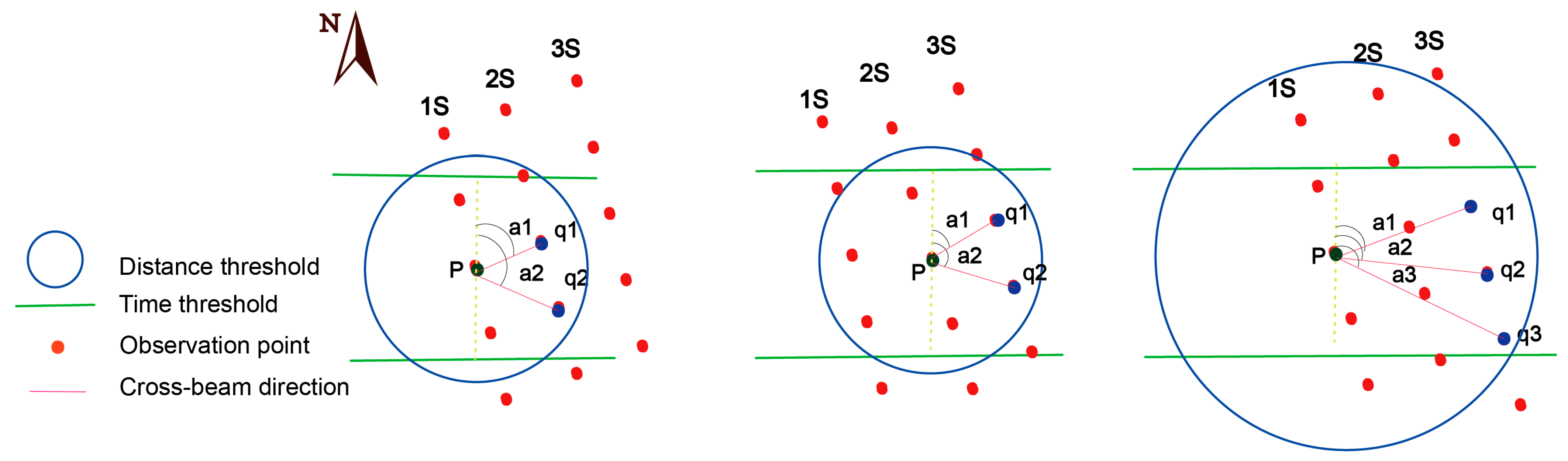
Remotesensing 15 00030 g003
Figure 4. Schematic diagram of calculation method for the cross-beam DOV (‘a1’, ‘a2’ and ‘a3’ is the azimuth of two adjacent observation points).
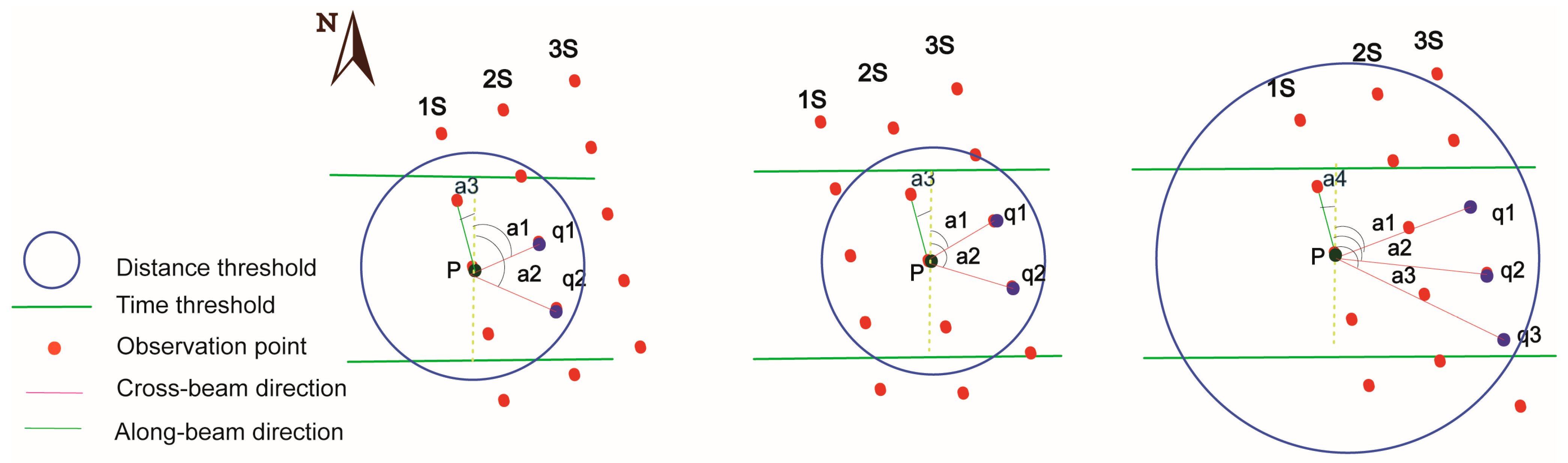
Remotesensing 15 00030 g004
Figure 5. Schematic diagram of calculation method for the joint along-cross beam DOV (‘a1’, ‘a2’, ‘a3’ and ‘a4’ is the azimuth of two adjacent observation points).
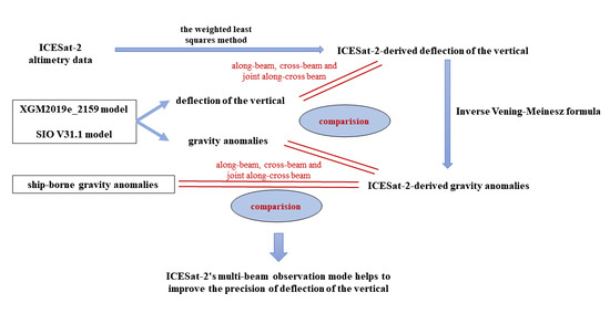
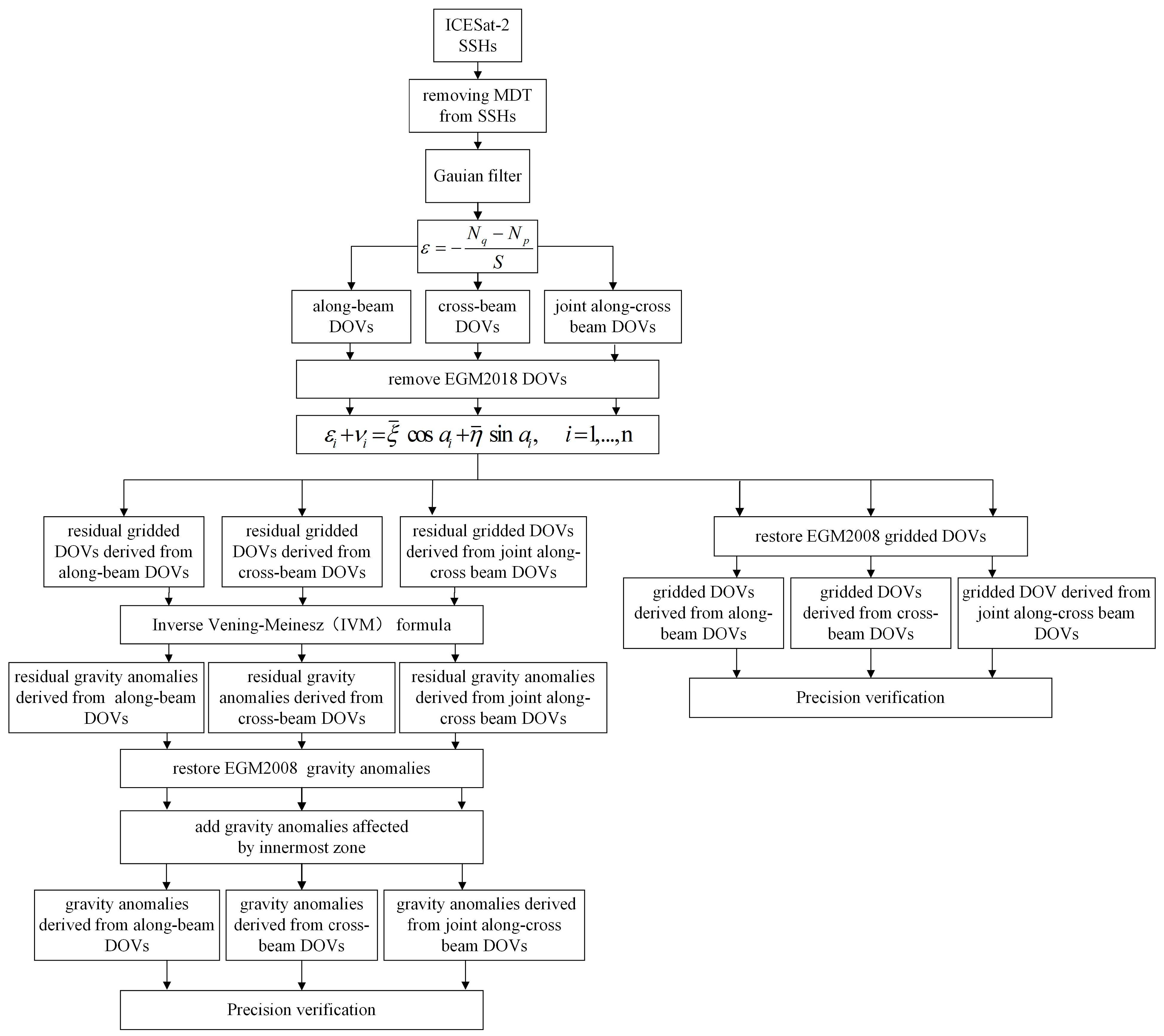
Remotesensing 15 00030 g005
Figure 6. Technical framework of deriving ICESat-2-derived deflection of the vertical with the weighted least squares method and gravity anomalies with the IVM formula.
Remotesensing 15 00030 g006
Figure 7. (a) The meridian component of the gridded DOV calculated by the ICESat-2 along-beam DOV; (b) the prime vertical component of the gridded DOV calculated by the ICESat-2 along-beam DOV.
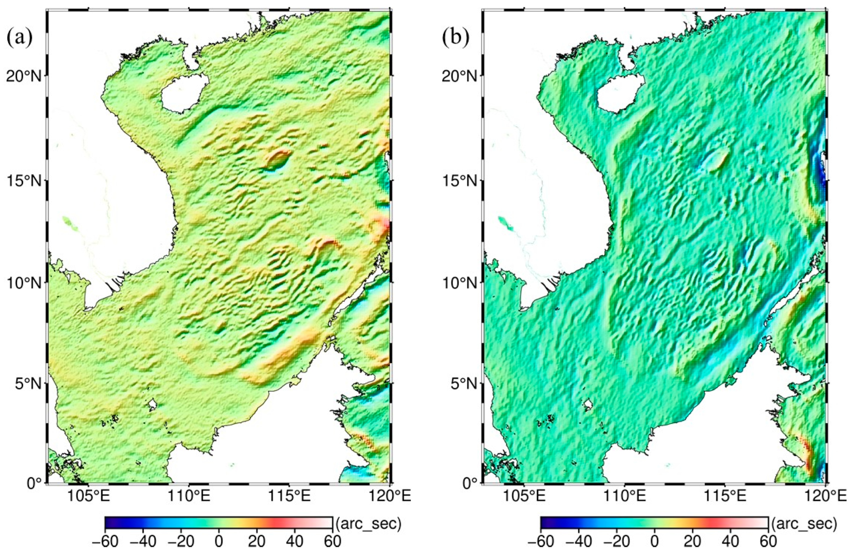
Remotesensing 15 00030 g007
Figure 8. (a) The meridian component of the gridded DOV calculated by the ICESat-2 cross-beam DOV; (b) the prime vertical component of the gridded DOV calculated by the ICESat-2 cross-beam DOV.
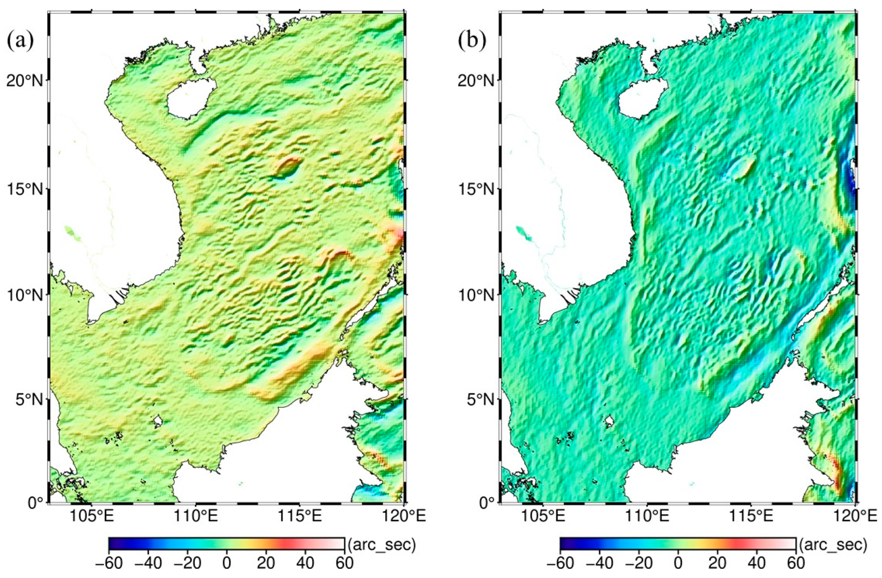
Remotesensing 15 00030 g008
Figure 9. (a) The meridian component of the gridded DOV calculated by the joint along-beam DOV; (b) the prime vertical component of the gridded DOV calculated by the joint along-beam DOV.
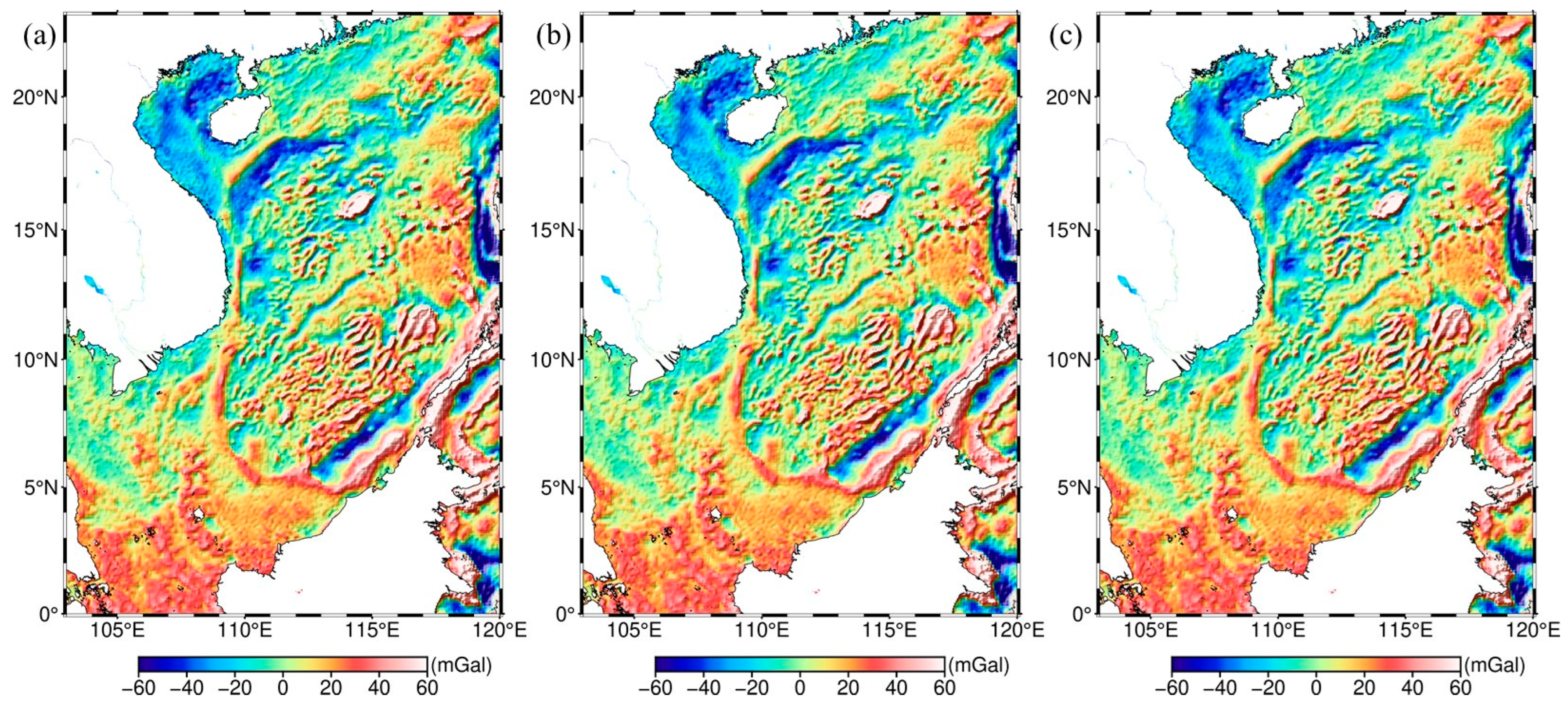
Remotesensing 15 00030 g009
Figure 10. (a) Gravity anomaly calculated by the along-beam DOV; (b) gravity anomaly calculated by the cross-beam DOV; (c) gravity anomaly calculated by the joint along-cross beam DOV.
Remotesensing 15 00030 g010
Table 1. The value of sc_orient corresponding to the strong-beam orientation at different times.
TimeSc_OrientStrong-Beam Orientation
2018.10.13–2018.12.281R
2018.12.28–2019.09.060L
2019.09.06–2020.05.141R
2020.05.14–2021.01.150L
2021.01.15–2021.07.151R
Table 2. Difference in SSHs at ICESat-2 and Jason-3 self-crossover points (Unit: cm).
Time ThresholdSatelliteNumMaxMinMeanStd
10 DaysICESat-2799038.99−34.750.058.23
Jason-3469121.92−21.820.017.52
91 DaysICESat-245,80349.94−49.76−0.7012.04
Jason-340,14537.47−37.050.0410.57
Without Time LimitICESat-2254,75349.99−49.98−1.5014.38
Jason-3227,60944.83−46.00−0.6212.16
Table 3. Differences in SSHs at the self-crossover points of ICESat-2 within 10 days (Unit: cm).
BeamNumMaxMinMeanStd
1L39528.64−44.68−0.668.17
2L35925.79−24.17−0.856.72
3L39848.66−26.14−1.107.10
1R51742.39−42.350.349.17
2R45149.17−28.360.498.69
3R51049.93−40.941.3710.13
Table 4. Differences in SSHs at the self-crossover points of ICESat-2 within 91 days (Unit: cm).
BeamNumMaxMinMeanStd
1L208644.04−49.76−1.2011.08
2L187547.07−47.96−1.0210.76
3L206348.66−47.71−1.1211.01
1R239349.45−48.17−0.7412.55
2R212549.17−49.39−0.2711.96
3R248449.93−49.510.0112.80
Table 5. Differences in SSHs at the self-crossover points of ICESat-2 without time limit (Unit: cm).
BeamNumMaxMinMeanStd
1L615449.53−49.91−4.2413.93
2L548547.52−49.63−4.2213.36
3L612749.61−49.52−3.9713.80
1R865849.45−49.900.0414.07
2R759349.98−49.390.0913.51
3R872549.43−49.88−0.3514.28
Table 6. Differences in SSHs at the cross-crossover points of ICESat-2 strong beam and Jason-3 (“A” represents the ascending orbit, “D” represents the descending orbit, “J3” represents Jason-3, and L/R and 1/2/3 represent the corresponding ICESat-2 beam) (Unit: cm).
BeamNumMaxMinMeanStd
1L_A&J3_A44,73243.67−68.25−12.3015.43
2L_A&J3_A41,37044.07−66.16−11.3815.04
3L_A&J3_A44,38442.84−65.68−11.4015.03
1R_A&J3_A55,03240.23−67.23−13.4114.58
2R_A&J3_A53,27041.23−68.79−13.8014.79
3R_A&J3_A56,04240.69−69.64−14.5014.97
1L_A&J3_D25,74095.53−118.48−12.7518.19
2L_A&J3_D24,255116.98−126.48−12.9518.02
3L_A&J3_D24,977114.06−139.28−11.6117.73
1R_A&J3_D31,51540.57−68.90−13.9115.17
2R_A&J3_D29,83040.27−70.39−14.9715.01
3R_A&J3_D32,47037.74−67.97−15.3415.02
1L_D&J3_A26,669123.69−166.76−13.5816.83
2L_D&J3_A25,10143.82−74.76−14.5015.13
3L_D&J3_A26,729142.46−174.37−14.0719.19
1R_D&J3_A32,20858.58−86.55−14.3815.25
2R_D&J3_A29,580109.02−140.91−14.5315.70
3R_D&J3_A32,01873.01−99.62−14.2516.16
1L_D&J3_D47,37742.97−68.52−13.1114.87
2L_D&J3_D44,44937.75−65.09−13.7014.68
3L_D&J3_D47,27550.61−76.98−13.5815.36
1R_D&J3_D55,13782.11−10.51−13.4916.52
2R_D&J3_D51,23576.24−102.83−14.1616.81
3R_D&J3_D54,88159.71−85.19−12.7315.85
Table 7. STD of differences between gravity anomalies derived by different Gaussian filter windows and NCEI ship-borne gravity anomalies (Unit: mGal).
σ /km 048
ICESat-2_ship4.564.524.57
Table 8. Statistics of differences between the along-beam DOVs and the XGM2019e_2159-DOV model (Unit: arc_sec).
BeamNumMaxMinMeanRmsStd
1L_XGM19196,0903.61−3.60−0.0021.091.09
2L_XGM19153,7913.38−3.37−0.0021.011.01
3L_XGM19190,8093.54−3.53−0.011.061.06
1R_XGM19174,2274.69−4.69−0.0011.121.12
2R_XGM19149,4593.44−3.43−0.011.021.02
3R_XGM19173,6783.73−3.72−0.011.131.13
ICESat-2_XGM191,069,6343.66−3.65−0.011.071.07
Table 9. STD of differences between gridded DOVs calculated by the along-beam DOVs with different search radii and the SIO V31.1_DOV model (Unit: arc_sec).
Search Radius 4′6′8′10′
ICESat-2_SIO-DOVMeridian1.261.231.211.27
Prime 4.584.544.534.55
Table 10. Statistics of differences between gridded DOVs calculated by the along-beam DOVs and the XGM2019e_2159-DOV model (Unit: arc_sec).
BeamDirectionMaxMinMeanRmsStd
1L_XGM19Meridian48.51−32.100.072.032.03
Prime 46.15−63.98−0.345.625.62
2L_XGM19Meridian35.64−37.790.092.312.31
Prime 38.70−50.70−0.375.655.65
3L_XGM19Meridian35.76−36.170.072.032.03
Prime 50.41−50.69−0.315.595.59
1R_XGM19Meridian32.65−26.400.031.331.33
Prime 37.91−46.12−0.235.125.12
2R_XGM19Meridian33.89−25.330.041.611.61
Prime 37.88−51.46−0.235.185.18
3R_XGM19Meridian32.08−24.140.031.461.46
Prime 38.97−51.90−0.285.215.21
ICESat-2_XGM19Meridian18.62−14.780.011.281.28
Prime 20.88−22.01−0.084.764.76
Table 11. Statistics of differences between gridded DOVs calculated by the along-beam DOVs and the SIO V31.1-DOV model (Unit: arc_sec).
BeamDirectionMaxMinMeanRmsStd
1L_SIOMeridian45.86−30.380.122.082.08
Prime 47.61−61.62−0.405.175.17
2L_SIOMeridian30.74−33.840.132.302.30
Prime 37.99−51.32−0.425.245.24
3L_SIOMeridian35.25−33.570.112.072.07
Prime 52.22−61.99−0.405.225.22
1R_SIOMeridian28.88−23.830.061.601.60
Prime 37.06−45.18−0.324.734.73
2R_SIOMeridian31.80−22.100.131.931.93
Prime 34.91−50.05−0.354.814.81
3R_SIOMeridian29.86−23.130.071.771.77
Prime 41.43−51.93−0.364.754.75
ICESat-2_SIOMeridian21.64−17.600.041.211.21
Prime 35.18−31.84−0.154.534.53
Table 12. Statistics of differences between the cross-beam DOVs and the XGM2019e_2159-DOV model (Unit: arc_sec).
BeamNumMaxMinMeanRmsStd
1L_2L_XGM19279,4396.95−7.21−0.112.242.24
2L_3L_XGM19274,5485.42−5.570.091.711.71
1L_3L_XGM19630,1384.00−4.21−0.101.251.25
1R_2R_XGM19209,3897.56−6.380.602.302.30
2R_3R_XGM19221,0069.66−9.95−0.153.263.26
1R_3R_XGM19492,3165.64−5.080.291.711.71
ICESat-2_XGM192,096,3816.19−6.100.051.891.89
Table 13. Statistics of differences between gridded DOVs calculated by the cross-beam DOVs and the XGM2019e_2159-DOV model (Unit: arc_sec).
BeamDirectionMaxMinMeanRmsStd
1L_2L_XGM19Meridian30.62−25.340.132.982.98
Prime 24.41−35.120.352.242.24
2L_3L_XGM19Meridian29.54−24.780.132.472.47
Prime 15.92−31.94−0.011.831.83
1L_3L_XGM19Meridian26.55−17.200.101.781.78
Prime 23.15−29.900.191.691.69
1R_2R_XGM19Meridian27.09−33.69−0.323.293.29
Prime 30.39−32.02−0.252.002.00
2R_3R_XGM19Meridian31.61−28.210.164.024.02
Prime 30.94−32.96−0.352.662.66
1R_3R_XGM19Meridian28.23−22.27−0.062.242.24
Prime 38.68−33.65−0.321.761.76
ICESat-2_XGM19Meridian20.14−17.690.011.741.74
Prime 24.56−29.49−0.011.601.60
Table 14. Statistics of differences between gridded DOVs calculated by the cross-beam DOVs and the SIO V31.1-DOV model (Unit: arc_sec).
BeamDirectionMaxMinMeanRmsStd
1L_2L_SIOMeridian25.26−18.770.172.722.72
Prime 38.87−33.630.332.192.19
2L_3L_SIOMeridian27.99−19.860.162.292.29
Prime 36.90−30.49−0.041.871.87
1L_3L_SIOMeridian23.20−16.760.161.731.73
Prime 36.90−30.490.131.661.66
1R_2R_SIOMeridian23.96−24.88−0.273.013.01
Prime 38.39−29.69−0.281.991.99
2R_3R_SIOMeridian32.71−25.860.193.663.66
Prime 36.31−30.63−0.382.622.62
1R_3R_SIOMeridian23.68−22.18−0.012.082.08
Prime 37.47−33.68−0.131.821.82
ICESat-2_SIOMeridian22.38−18.730.041.701.70
Prime 12.02−12.21−0.031.581.58
Table 15. Statistics of differences between the joint along-cross DOV and the XGM2019e_2159-DOV model (Unit: arc_sec).
BeamBeam GroupNumMaxMinMeanRmsStd
1L1L_2L475,0376.04−5.890.051.831.83
1L1L_3L826,8984.18−4.020.081.261.26
2L2L_3L428,6984.99−4.890.071.511.51
1R1R_2R395,8405.50−6.13−0.311.821.82
1R1R_3R679,5244.87−5.29−0.221.611.61
2R2R_3R370,3318.00−7.840.092.542.54
Along-Beam Cross-beam 3,163,5185.46−5.400.031.631.63
Table 16. Statistics of differences between gridded DOVs calculated by the joint along-cross beam DOVs and the XGM2019e_2159-DOV model (Unit: arc_sec).
BeamBeam GroupDirectionMaxMinMeanRmsStd
1L1L_2LMeridian20.74−19.910.020.940.94
Prime 24.64−38.130.362.212.21
1L1L_3LMeridian30.35−16.590.031.011.01
Prime 23.29−32.170.201.651.65
2L2L_3LMeridian29.65−17.670.020.930.93
Prime 18.15−45.09−0.011.791.79
1R1R_2RMeridian18.62−12.17−0.020.860.86
Prime 39.13−32.17−0.241.971.97
1R1R_3RMeridian19.85−18.08−0.020.950.95
Prime 38.70−33.72−0.331.751.75
2R2R_3RMeridian18.47−13.740.020.870.87
Prime 36.94−33.29−0.342.642.64
Along-Beam Cross-beam Meridian15.14−14.790.010.840.84
Prime 16.79−17.08−0.121.551.55
Table 17. Statistics of differences between gridded DOVs calculated by the joint along-cross beam DOVs and the SIO V31.1_DOV model (Unit: arc_sec).
BeamBeam GroupDirectionMaxMinMeanRmsStd
1L1L_2LMeridian26.03−18.720.060.960.96
Prime 39.07−40.210.302.152.15
1L1L_3LMeridian25.87−16.630.071.011.01
Prime 37.00−32.250.161.641.64
2L2L_3LMeridian21.96−16.550.050.920.92
Prime 35.44−35.27−0.061.851.85
1R1R_2RMeridian30.39−16.860.010.860.86
Prime 37.28−29.84−0.281.981.98
1R1R_3RMeridian18.49−18.570.020.920.92
Prime 36.93−33.75−0.381.801.80
2R2R_3RMeridian20.47−17.000.060.860.86
Prime 35.51−30.96−0.402.612.61
Along-BeamCross-beam Meridian17.36−15.700.040.800.80
Prime 38.31−29.34−0.031.511.51
Table 18. Statistics of differences between the along-beam DOV-derived gravity anomalies and the XGM2019e_2159-GRA model, SIO V31.1-GRA model, and ship-borne gravity anomaly data (Unit: mGal).
NumMaxMinMeanRmsStd
ICESat-2_XGM19231,65526.02−25.580.182.762.76
ICESat-2_SIO243,97536.32−37.18−0.044.094.09
ICESat-2_ship289,16643.36−45.34−0.105.345.34
Table 19. Statistics of differences between the cross-beam DOV-derived gravity anomalies and the XGM2019e_2159-GRA model, SIO V31.1-GRA model, and ship-borne gravity anomaly data (Unit: mGal).
NumMaxMinMeanRmsStd
ICESat-2_XGM19231,65532.16−34.550.163.813.81
ICESat-2_SIO243,97539.14−39.85−0.023.833.83
ICESat-2_ship289,16640.19−40.52−0.054.934.93
Table 20. Statistics of differences between the joint along-cross DOV-derived gravity anomalies and the XGM2019e_2159-GRA model, SIO V31.1-GRA model, and ship-borne gravity anomaly data (Unit: mGal).
NumMaxMinMeanRmsStd
ICESat-2_XGM19231,65535.89−37.540.162.492.49
ICESat-2_SIO243,97539.61−40.86−0.023.063.06
ICESat-2_ship289,16641.63−42.36−0.054.414.41
Disclaimer/Publisher’s Note: The statements, opinions and data contained in all publications are solely those of the individual author(s) and contributor(s) and not of MDPI and/or the editor(s). MDPI and/or the editor(s) disclaim responsibility for any injury to people or property resulting from any ideas, methods, instructions or products referred to in the content.

