Improving the Operational Simplified Surface Energy Balance Evapotranspiration Model Using the Forcing and Normalizing Operation

Abstract

Actual evapotranspiration modeling is providing useful information for researchers and resource managers in agriculture and water resources around the world. The performance of models depends on the accuracy of forcing inputs and model parameters. We developed an improved approach to the parameterization of the Operational Simplified Surface Energy Balance (SSEBop) model using the Forcing and Normalizing Operation (FANO). SSEBop has two key model parameters that define the model boundary conditions. The FANO algorithm computes the wet-bulb boundary condition using a linear FANO Equation relating surface temperature, surface psychrometric constant, and the Normalized Difference Vegetation Index (NDVI). The FANO parameterization was implemented on two computing platforms using Landsat and gridded meteorological datasets: (1) Google Earth Engine (GEE) and (2) Earth Resources Observation and Science (EROS) Center Science Processing Architecture (ESPA). Evaluation was conducted by comparing modeled actual evapotranspiration (ETa) estimates with AmeriFlux eddy covariance (EC) and water balance ETa from level-8 Hydrologic Unit Code sub-basins in the conterminous United States. FANO brought substantial improvements in model accuracy and operational implementation. Compared to the earlier version (v0.1.7), SSEBop FANO (v0.2.6) reduced grassland bias from 47% to −2% while maintaining comparable bias for croplands (11% versus −7%) against EC data. A water balance-based ETa bias evaluation showed an overall improvement from 7% to −1%. Climatology versus annual gridded reference evapotranspiration (ETr) produced comparable ETa results, justifying the use of climatology ETr for the global SSEBop Landsat ETa that is accessible through the ESPA website. Besides improvements in model accuracy, SSEBop FANO increases the spatiotemporal coverage of ET modeling due to the elimination of high NDVI requirements for model parameterization. Because of the existence of potential biases from forcing inputs and model parameters, continued evaluation and bias corrections are necessary to improve the absolute magnitude of ETa for localized water budget applications.

1. Introduction

Evapotranspiration (ET) estimation and mapping over large areas and longer time frames has become an active applied research activity in recent years with the use of satellite-derived inputs and the availability of global weather datasets. The level of complexity of the various models can be broadly described as ranging from parametric- to process-based approaches. The parametric models estimate actual evapotranspiration (ETa) by decomposing actual ET into independent parameters such as potential evapotranspiration and factors that account for the limiting conditions [1,2,3,4,5,6]. The process-based models are either based on mass balance approaches [7,8,9,10] used by prognostic hydrologic/biophysical models or full energy balance approaches used by diagnostic ET models [11,12,13,14]. Models require the estimation of parameters whose level of complexity tends to increase from parametric- to process-based models [15]. Depending on the modeling principles, parameters generally define model boundary conditions, control flux rates, or storage terms. With a growing interest for global field-scale ETa within a time scale of agro-climatic decision-making processes in agriculture and water resources, ETa modelers are expected to produce accurate, consistent, and useful ET datasets. Modelers are continuously updating their models for accuracy and computational efficiency as new input datasets, techniques, or model parameterization schemes become available.

One of the models that is being used for operational global ETa mapping is the Operational Simplified Surface Energy Balance (SSEBop) model [16]. SSEBop is being used for field-scale and basin-wide estimation of ETa along for updating historical records (e.g., Senay et al. [17,18], Schauer and Senay [19]). SSEBop is a parametric energy balance-based model that treats actual ET as a product of two independently estimated quantities: (1) ET fraction (ETf) and (2) the maximum ET under water-unlimited environmental conditions (Equation (1)):

ETa = ETf · ETr

(1)

where ETa is actual ET (mm) and ETr is alfalfa-reference (“maximum/potential”) ET (mm).

ETf is estimated from the observed satellite land surface temperature (Ts) using the concept of satellite psychrometry that uses two model parameters to define the model boundary conditions for minimum and maximum ET (Equation (2)) [6], expressed as:

ETf = 1 − γ^s(Ts − Tc)

(2)

where ETf is the daily ET fraction (0.0–1.0) for each pixel; γ^s is the surface psychrometric constant over a dry-bare surface and is the same as the inverse of the dT (temperature difference, K) parameter in Senay et al. [15]; Ts is the dry-bulb surface temperature (K) derived from the satellite thermal infrared band, and Tc is the wet-bulb reference surface temperature (K) limit; The constant 1 represents the ET fraction value during maximum ETa, i.e., when Ts = Tc.

The surface psychrometric constant (γ^s) is determined based on energy balance principles. The γ^s parameter was calculated using data from ERA5 (5th generation European Center for Medium-Range Weather Forecasts Reanalysis) for the primary inputs of net radiation parameters [16] and is available for the globe [17].

Here, we present the formulation of an improved parameterization scheme for the SSEBop model in the estimation of the Tc parameter using an innovative analytical solution. The main innovation involves the elimination of the high NDVI (Normalized Difference Vegetation Index) requirement and replacing it with a deterministic equation that expands the spatiotemporal coverage of the SSEBop model. While γ^s may be assumed constant for a given location (1 km × 1 km) and day-of-year, Tc is considered spatiotemporally dynamic and must be determined for each satellite overpass. Earlier versions of SSEBop determined Tc by identifying dense green vegetation using the NDVI (>0.7) and corresponding land surface temperature (Ts) to calibrate the air temperature for establishing Tc for each overpass image (Senay et al. [18]; Senay [6]). Although this approach worked adequately for images with sufficient calibration points (high NDVI), there were at least three major limitations: (1) high NDVI images that meet the NDVI > 0.7 criterion may not be available in arid and semi-arid regions or outside of major growing seasons in different parts of the world, (2) high NDVI calibration landscapes are not uniformly distributed in a given image, thus extrapolating Tc to the entire image from isolated calibration points could introduce errors in hydro-climatically complex regions, and (3) the NDVI threshold could create widely varying Tc ranges because some images may only have a narrow range of NDVI that is closer to the threshold (NDVI = 0.7) while others may have Tc values derived from pixels with NDVI far higher than the 0.7 threshold (e.g., NDVI = 0.9). The difference in Ts between NDVI 0.7 and 0.9 could be as high as 4 to 5 K [16].

To estimate ETa in all landscapes and all seasons regardless of vegetation cover density and to improve model accuracy by avoiding extrapolation of Tc to non-calibration regions, a new parameterization algorithm is developed for determining Tc. The algorithm follows a Forcing and Normalizing Operation (FANO): every pixel in the landscape is forced to have its own Tc using an algebraic equation that requires a normalization operation as described below.

The main objectives of this study are: (1) outline the formulation of the FANO parameterization in SSEBop, (2) describe the implementation of the updated model in two computing platforms, (3) present evaluation results using station-based ET measurements and water balance ET approaches, and (4) feature illustrative ET maps in different parts of the world.

2. Methods

2.1. Auxiliary Data

Auxiliary inputs to the SSEBop ETa modeling include maximum air temperature (Ta), inverse of the psychrometric constant (dT), and alfalfa-reference evapotranspiration (ETr). The SSEBop model uses long-term climatological datasets for each of these variables. The dT dataset is created from ERA5 radiation data along with other weather variables and condensed into a daily median [17]. The maximum air temperature is the 1981–2010 climatological normal (30-year daily mean) and is a combination of two datasets: Daymet Version 4 for North America and CHELSA Version 2 for the globe outside of North America [19,20]. Both the dT and Ta datasets are at 1 km resolution. The ETr is also a 1981–2010 climatological normal but is a fusion of different model assimilated products.

Over the conterminous United States (CONUS), the 1981–2010 daily ETr of Gridmet is used and scaled by a factor of 0.85 to reduce the generally high bias from Gridmet [21]. The Gridmet ETr is at 4 km resolution in CONUS. For areas outside of CONUS, coarser resolution (refined to 12 km) ETr is utilized, which is derived from the MERRA-2 (Modern-Era Retrospective analysis for Research and Applications) data and processed by the National Oceanic and Atmospheric Administration (NOAA) Physical Sciences Laboratory [22]. The MERRA-2 ETr was scaled to match the relative magnitudes of Gridmet by utilizing the WorldClim Version 3 Potential Evapotranspiration dataset (ETr). The WorldClim Version 3 ETr is a climatological dataset from 1970–2000. Terrestrial ecoregions for 2017 from the One Earth/RESOLVE organization were used to scale the ETr [23,24]. These datasets were combined to determine a daily global ETr dataset with Gridmet ETr over CONUS and MERRA-2 ETr for all areas outside CONUS. The areas outside of CONUS were scaled for each ecoregion, smoothed, and resampled to 1 km resolution [25].

2.2. FANO Illustration: Data and Development

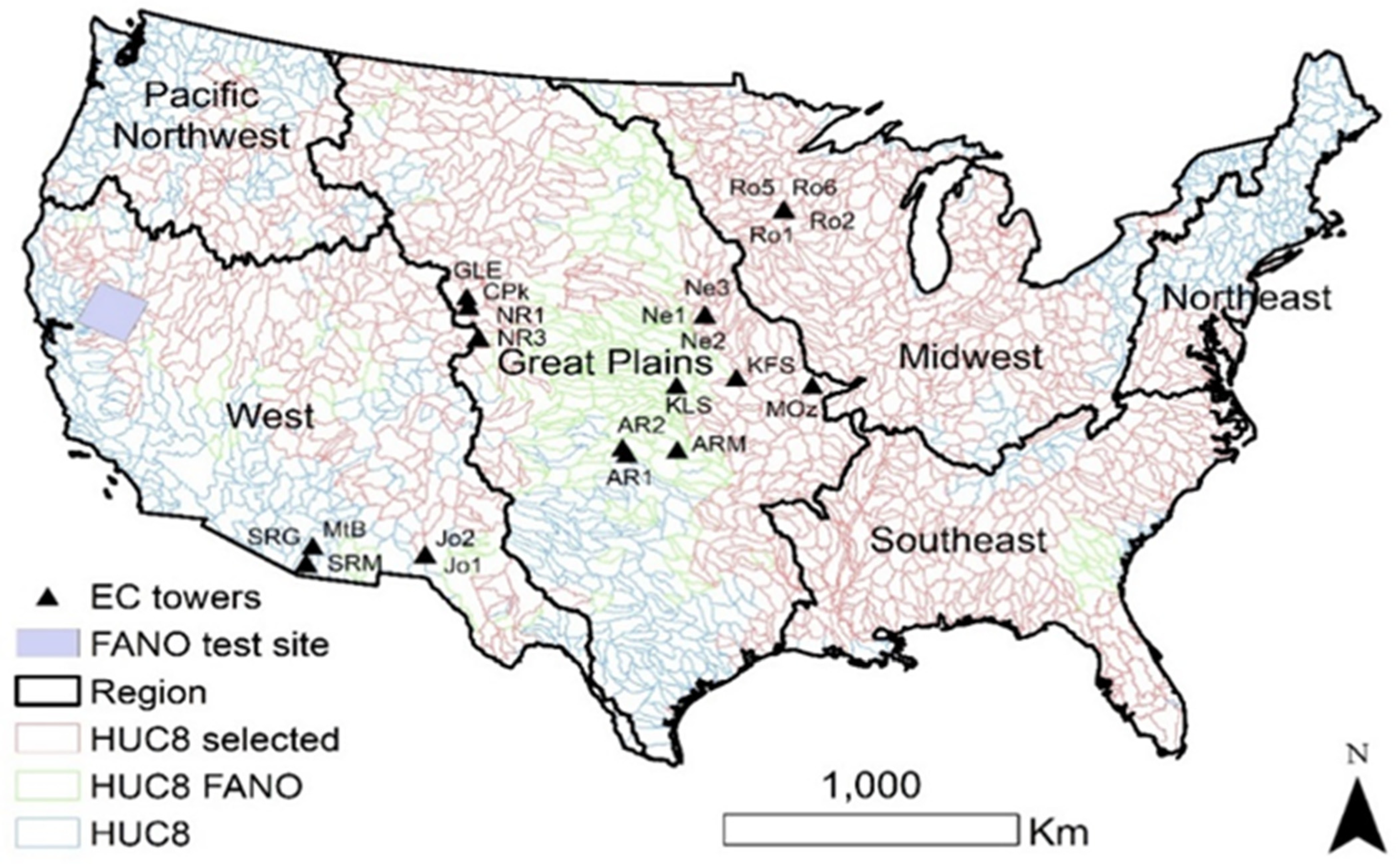
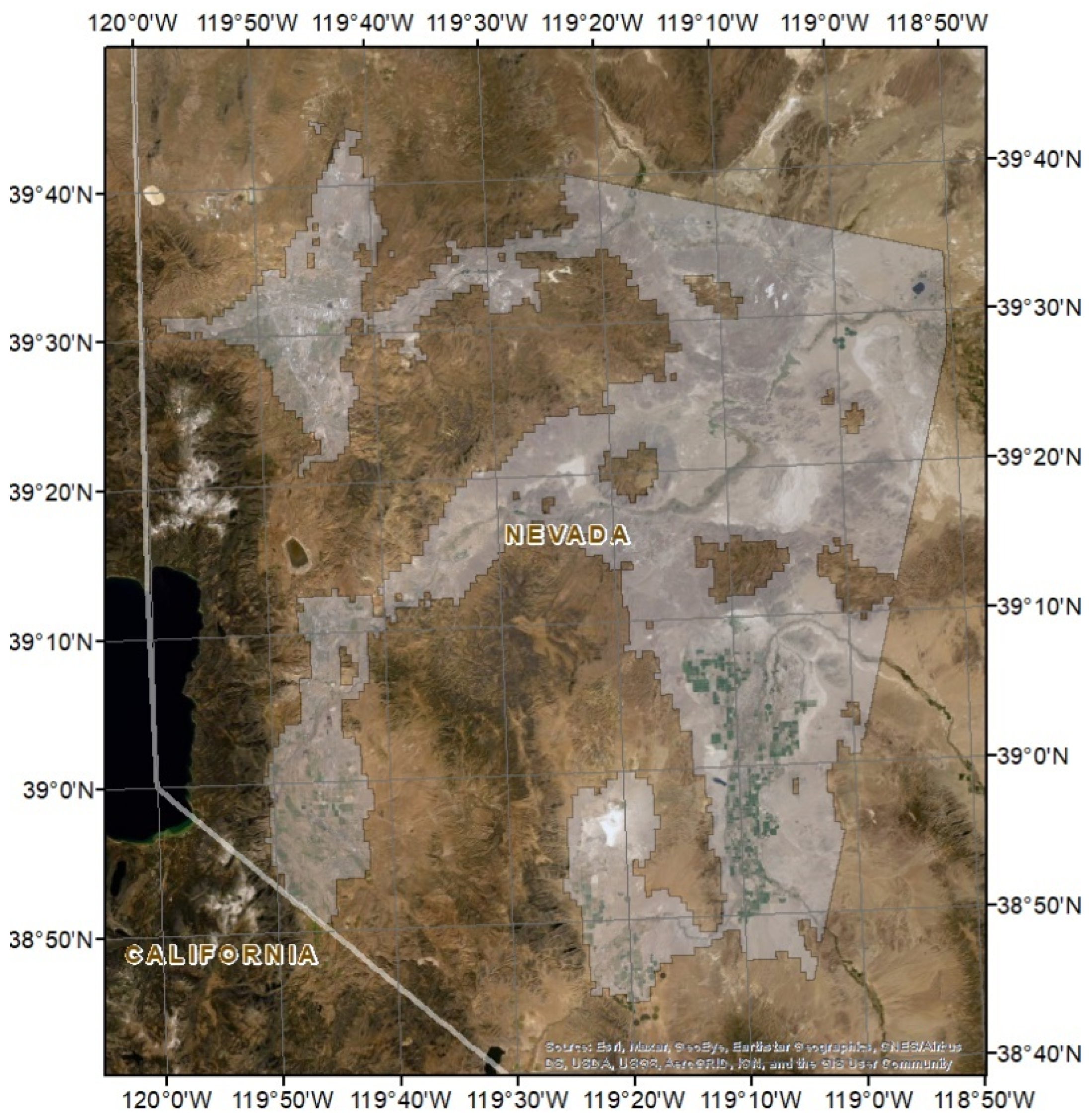
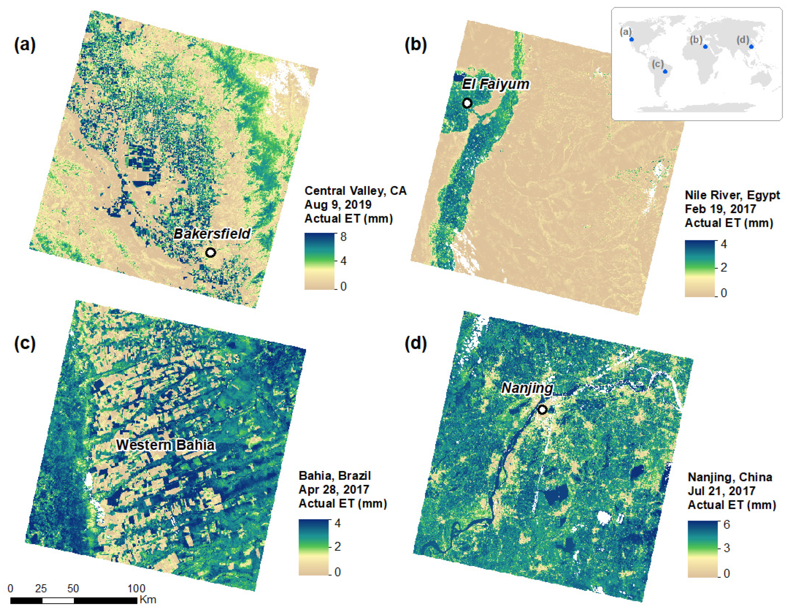
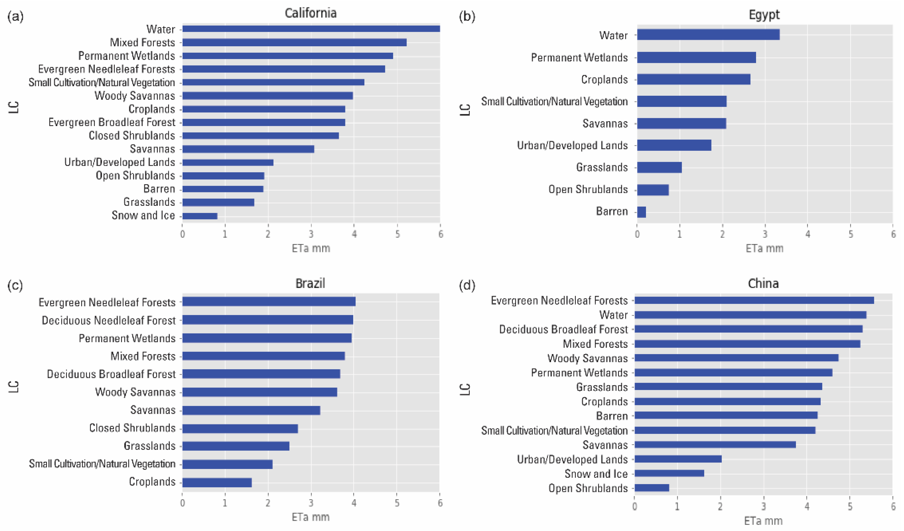
We propose a linear relation between a normalized land surface temperature difference and NDVI difference using the dT parameter and a proportionality constant (Equation (3)). This governing equation is named “Senay Approximation,” after the primary author who formulated it in this study:

$$\frac{\Delta T{s}^{*}}{d{T}^{*}}=-f·\Delta NDV{I}^{*}$$

(3)

where * denotes a large area (~5 km) average value of the parameter in question; ΔTs^* represents the expected land surface temperature difference (K) between the observed Ts (spatial average) and expected wet-bulb (Tc); ΔNDVI^* is the NDVI difference between the observed (spatial average) and theoretical maximum NDVI of 0.9 that would correspond to the wet-bulb pixels; dT^* is the inverse of the surface psychrometric constant that defines the temperature difference between a dry-bare surface and the canopy level air temperature [6]; f is a proportionality “FANO” constant formulated in this study that relates the ratio ΔTs^*/dT^* to ΔNDVI^*. The negative sign indicates the known inverse relation between Ts and NDVI, which translates into a smaller ΔTs at high NDVI and a larger ΔTs at lower NDVI surfaces.

It is important to note that the left side of Equation (3) is the same form as the ETf in Equation (2) without the constant term 1 and is equivalent to a sensible heat fraction (Hf), assuming a negligible ground heat flux at a daily time scale. Simply, the Senay Approximation states that over a large area, the average ETf or Hf is linearly related to changes in NDVI (from maximum) for all seasons and locations with a proportionality constant f and this relationship can be used to determine the wet-bulb land surface temperature, Tc.

In this study a “global” average value for f of 1.25 was used as described below. This value can be more accurately determined by plotting the ratio ΔTs/dT against ΔNDVI for a more localized application. The large-area average requirement denoted by * indicates the importance of spatial scale in the established linear relationship.

2.2.1. Study Area

The determination of the FANO constant f requires the gathering of empirical data in different parts of the world. Below is an example obtained from a study site by Carson City, Nevada, United States (Figure 1 and Figure 2). It is important to note that the form of the FANO formulation (Equation (3)) is theoretical and thus not tied to the empirical data from the study site. The lack of observed data from multiple sites should only affect the determination of the magnitude of f and its variability in space and time, which requires an independent study.

Landsat 8 data, acquired on 1 July 2020 from path/row 043/033, covering the western part of Nevada in the United States (Figure 1), was used for Ts and NDVI. The image was chosen due to various levels of irrigation and vegetation condition to have a good range of NDVI and Ts distribution. To keep the effect of elevation on Ts to the minimum level, we used a digital elevation model (DEM) [26] to sample NDVI and Ts within a relatively narrow range of elevation between 1200 m and 1500 m. The temperature difference dT (25.25 K) for the same day was extracted for the study area from the global dT dataset [17].

The Landsat image was grouped into nine bins using a 0.1 NDVI interval from 0.05 to 1.0 except the last bin with an interval of 0.15 because of the rarity of pixels with NDVI > 0.95. In each bin, the spatial average of NDVI and Ts were calculated, yielding NDVI^* and Ts^*, respectively. The Ts magnitude within the NDVI bin of 0.85–1.0 was considered to represent the wet-bulb with a value of 302.2 K (

Table 1. Spatial-average values for Landsat NDVI and Ts, and dT parameters corresponding to the 1 July 2020, image. Pixel count refers to the number of 30 m pixels for each parameter. The * indicates spatial averages for each NDVI bin.

NDVI Bin	Pixel Count	NDVI*	dT*	Ts*	ΔTs*	ΔNDVI*	ΔTs*/dT*
0.05–0.15	2,249,526	0.11	25.26	327.5	25.3	−0.79	1.00
0.15–0.25	639,361	0.18	25.26	324.8	22.6	−0.72	0.90
0.25–0.35	174,131	0.29	25.26	320.2	18.0	−0.61	0.71
0.35–0.45	140,212	0.39	25.26	317.3	15.0	−0.51	0.60
0.45–0.55	118,247	0.50	25.26	314.7	12.5	−0.40	0.49
0.55–0.65	104,927	0.61	25.26	311.5	9.2	−0.29	0.37
0.65–0.75	78,558	0.73	25.26	308.3	6.1	−0.17	0.24
0.75–0.85	57,827	0.82	25.26	305.2	3.0	−0.08	0.12
0.85–1.00	26,426	0.89	25.26	302.2	0.00	−0.01	0.00

). The maximum NDVI associated with the wet-bulb Ts was set to be 0.9 when using surface reflectance-based NDVI. The derivation of the change in NDVI (ΔNDVI^*) and the normalization of change in Ts using dT (i.e., ΔTs*/dT^*) is described below.

The pixel count for each of the bins ranged from 26,426 to 2,249,526, which corresponds to about 24 km² (highest NDVI bin) to 2025 km² (lowest NDVI bin), respectively (Table 1). This ensures a reliable average value for NDVI and Ts regardless of differences in the number of pixels among the different NDVI bins. The average NDVI ranged from 0.11 in the lowest bin to 0.89 in the highest bin with the corresponding Ts^* varying from 327.5 K to 302.2 K yielding a difference of 25.3 K between the extreme NDVI bins. This observed Ts difference between the low and high NDVI locations within the study site (Figure 2) is coincidentally very close to the theoretically derived dT value of 25.26 K (Table 1). Figure 3 shows the temporal variability of dT for the study site with a peak (~25 K) in the summer and a minimum in the winter (~7 K).

Figure 4 illustrates the strong inverse linear relation between ∆Ts^*/dT^* and ∆NDVI^* created using an NDVImax = 0.9 and dT = 25.25 K. The FANO constant f is shown to be 1.23 in this example. However, f is expected to vary among samples (exploratory analysis shows a possible range between 1.10 and 1.40), but an average value of 1.25 is expected to provide a reasonable estimate for general and operational applications. The difference between f = 1.25 and f = 1.10 or between f = 1.25 and f = 1.40 is expected to result in an absolute error of 2 K in the estimation of Tc at low NDVI (0.3) landscapes or only an error of 1 K at high NDVI (0.6) landscapes, which is close to the uncertainty of the Land Surface Temperature and its effect on ETa estimation is relatively small.

According to Figure 4, the normalized Ts difference (∆Ts^* /dT^*) is expected to be 0.0 when the average NDVI is 0.9 because the maximum NDVI is expected to be 0.9. In the SSEBop formulation, ∆Ts^*/dT^* is the same as 1.0−ETf or simply the sensible heat fraction, Hf, in which case a minimum Hf (0.0) and maximum ETf (1.0) is attained at NDVI^* = 0.9. For example, at NDVI^* = 0.1, ∆NDVI^* is 0.8 which translates to ∆Ts^*/dT^* = 0.98 using the y = −1.23x Equation in Figure 4. Thus, Hf is high, close to 1.0, which indicates a negligible ETf around 0.02.

The next sections describe a generalized FANO Equation, which is expected to apply to all hydro-climatic conditions for any remotely sensed image collection that produces Ts and NDVI.

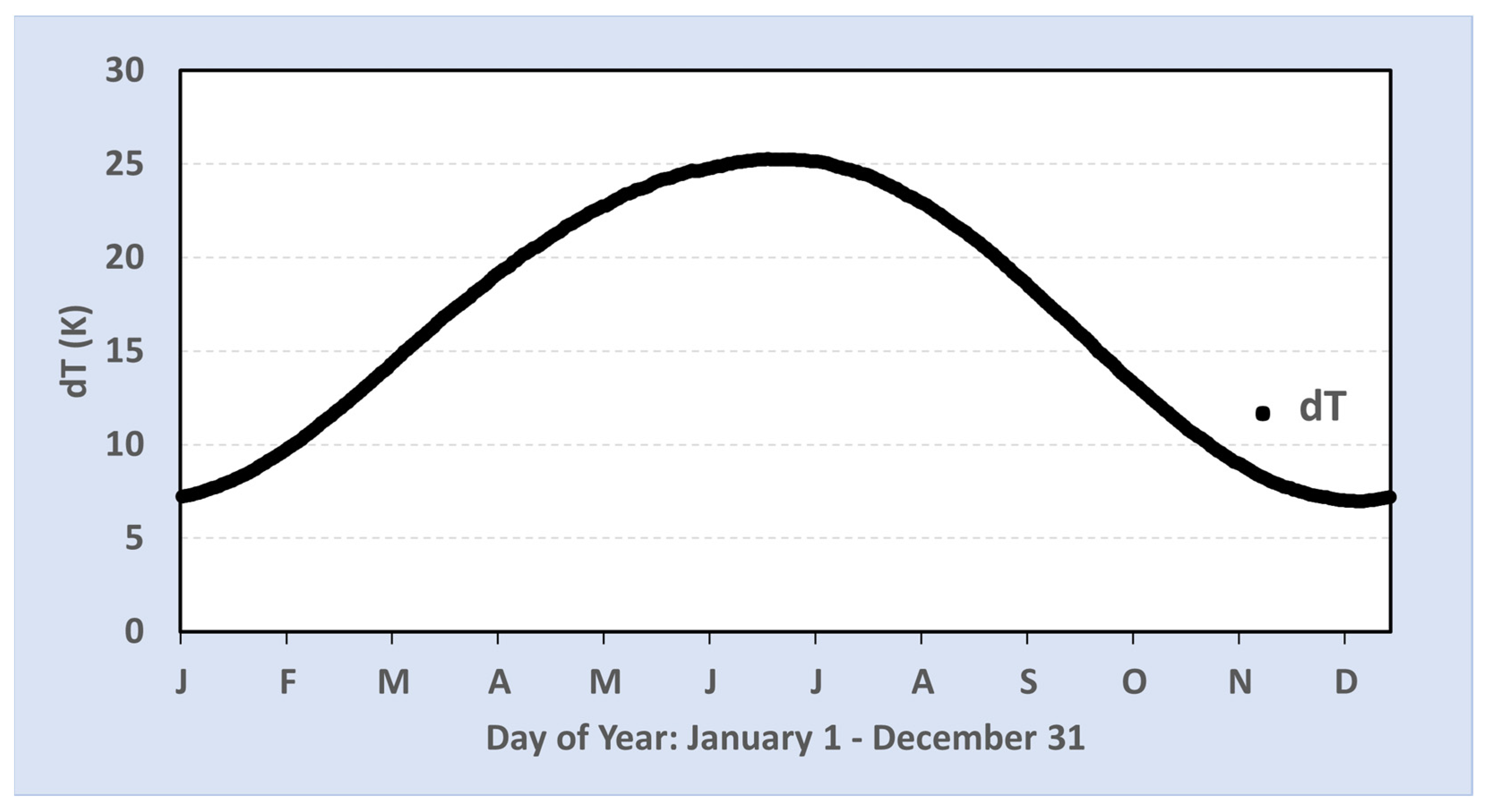
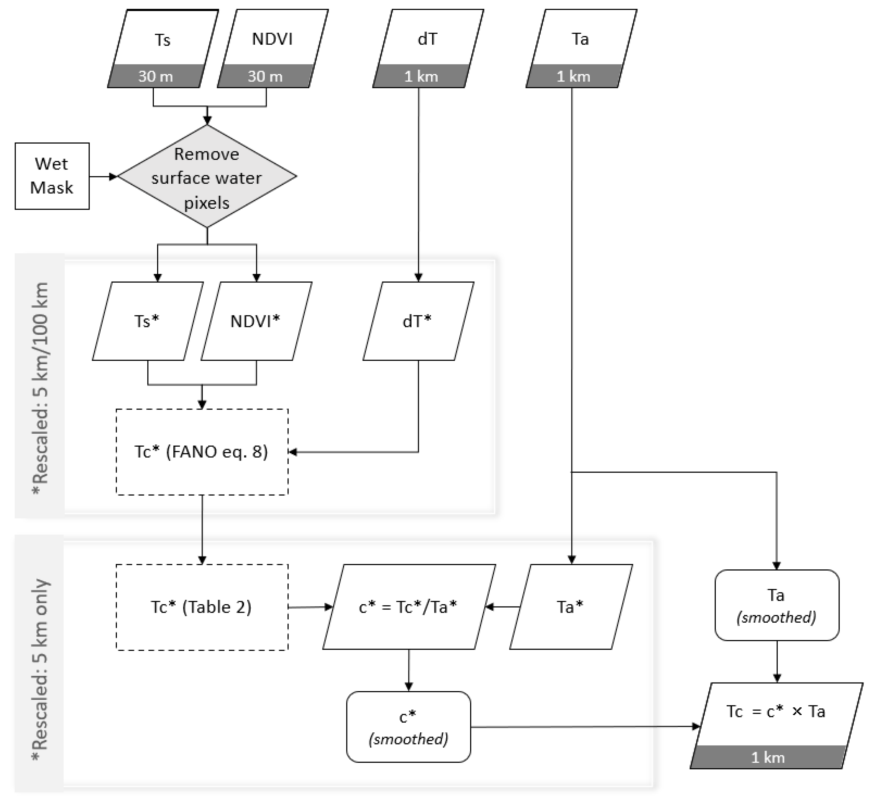
2.2.2. Forcing Operation in FANO: Tc Determination

Following Equation (3), a normalizing operation is required to establish a stable linear relationship through the averaging of parameters.

∆Ts^* = −f∙dT^* · ∆NDVI^*

(4)

By definition,

∆Ts^* = Ts^* − Tc^*

(5)

where Tc^* is the expected (ideal) wet-bulb (cold) reference surface temperature (K) at maximum NDVI (NDVImax) over a grid that includes the “warm” surface temperature (Ts^*); Ts^* is the observed warm surface temperature over a chosen grid size. This is designated as warm surface temperature because it represents the landscape surface temperature with an average NDVI most likely lower than the ideal NDVImax that could correspond to the reference wet-bulb (cold) temperature.

For averaging Ts and NDVI, we use a 5 km × 5 km grid size for Landsat. The size of the grid is determined by the stability of the relation between NDVI and Ts. If it is too small, the expected linear relationship may not hold due to differences in the inherent pixel size and co-registration issues between the thermal and NDVI datasets. Furthermore, other confounding factors such as partial cloud contamination and haze that affect the thermal infrared and NDVI bands differently would introduce random errors in the relationship. Thus, the average over a relatively large grid size is recommended. However, if the grid size is too large, the relationship may also be affected by other confounding factors such as elevation and latitude that affect the NDVI and Ts differently as well as different ecoregions such as valleys and mountains. In this study, grid sizes of 1, 3, 5, 10, 25, 50, 100 km were evaluated for Landsat, and the 5 km was found to show a more natural variation in space although the differences among the different sizes was not too large, validating the stability of the relation between averaged NDVI and Ts over different spatial scales. The change in NDVI is calculated from a maximum NDVI (Equation (6)).

∆NDVI^* = NDVI^* − NDVImax

(6)

where NDVImax represents an ideal maximum NDVI constant that corresponds to an ideal wet-bulb surface temperature (Tc^*); NDVI^* is the spatial-average observed NDVI (5 km × 5 km) that corresponds to the observed warm surface temperature (Ts^*).

In this study, the NDVImax from Landsat surface reflectance (SR) data was assumed to be NDVI = 0.9. On a separate investigation (data not shown) involving multiple scenes, the top-of-atmosphere (TOA) NDVI was found to be about 12% lower than the SR NDVI for the same vegetation cover; thus, adjusting the threshold values is necessary when using TOA NDVI.

Once the average values for NDVI, dT, and Ts are established, Tc^* can be estimated from an algebraic rearrangement of Equation (3) (Senay Approximation) by combining Equations (4)–(6), leading to the FANO Equation

Tc^* = Ts^* − f∙dT^*(NDVImax − NDVI^*)

(7)

Using optimized values of 1.25 for f and 0.9 for NDVImax, the FANO Equation is simplified to:

Tc^* = Ts^* − 1.25dT^*(0.9 − NDVI^*)

(8)

Thus, Equation (8), hereafter referred to as the FANO Equation, can be used to predict the average Tc^* from the observed Ts, NDVI, and predefined dT for any location and date without requiring knowledge of high NDVI calibration points unlike the previous versions of SSEBop. The following sections will also show the procedures used to determine higher resolution (~1 km) Tc from coarse resolution Tc^* (~5 km) using a c factor, like the earlier version of SSEBop [18].

2.2.3. Normalizing Operation in FANO: Parameter and Spatial Scale

The forcing and normalizing operations occur simultaneously. The FANO implementation has two key procedures: (1) because the slope between Ts and NDVI varies by season, the normalization of ∆Ts by dT allows a season- and location-independent relationship, and (2) because the relation between Ts and NDVI tends to be dispersed due to pixel size differences and other confounding factors, only an average over a relatively large area is expected to dampen the effect of random errors and establish a stable linear relationship. Thus, key input parameters for the FANO Equation were averaged over a large area. As noted above, 5 km is recommended in this study. Unlike the observed Ts, the predicted wet-bulb Tc is expected to be unform over a large area; thus, the use of an average over 5 km is justified.

FANO assumes an inverse linear relation between Ts and NDVI; thus, landscapes that violate this assumption will be filtered out before spatial averaging of Ts, NDVI, and dT for use in FANO. These surfaces are generally water bodies and wetlands where low NDVI is associated with low Ts. We used a combination of Landsat Quality bands, NDVI, and the Modified Normalized Difference Wetness Index (MNDWI) [27] to identify “wet” (surface water and/or wetlands) pixels and remove these pixels from the averaging (see “Wet Mask” in Figure 5). In each 5 km × 5 km grid, if more than 10% of the pixels are identified as wet, the averaging is conducted over a much larger area at 100 km × 100 km after excluding the wet pixels (see

Table 2. NDVI-based filtering procedures for FANO parameterization. Priority in the outcome is ranked from highest (“a”) to lowest (“d”).

Landscape Condition	Filtering Condition	Temperature Assignment	Outcome (priority)
FANO land condition	(0 ≤ NDVI* ≤ 0.9)	Tc* = Tc*5km	FANO at 5 km resolution (d)
FANO wet condition	(0 ≤ NDVI* ≤ 0.9) & (wet pixels > 10% in 5 km grid)	Tc* = Tc*100km	FANO at 100 km resolution (c)
Surface water	Unmasked NDVI* < 0	Tc* = Ts*	Water pixels retain average surface temperature (b)
Dense green vegetation	NDVI* > 0.9	Tc* = Ts*	High NDVI pixels retain average surface temperature (a)

). This procedure is particularly important over expansive coastal wetlands and rice growing regions. The larger area window increases the opportunity to find an adequate number of non-wet pixels to be used for the determination of Tc^* with FANO.

The FANO flowchart in Figure 5 illustrates how the different inputs (Ts, NDVI, dT, and Ta) are filtered, averaged, and ultimately applied to the FANO Equation to determine Tc^*. However, certain conditions, such as low NDVI associated with low Ts^* from water bodies and wetlands or high NDVI above the NDVI value of 0.9 require Ts values that have not been adjusted via the FANO Equation. The assumption here is that these are already representative of the wet-bulb condition and that Tc^* should be determined using an un-adjusted Ts^*. Referring to Table 2, we note that 5 km pixels that correspond to surface water conditions (NDVI^* < 0) are assigned Ts^* that does not mask out the water pixels. This is a wet-bulb condition; therefore, masking is not necessary. Conditions where NDVI^* > 0.9 (average over 5 km × 5 km) are exceedingly rare. However, if that is encountered, the pixels are assigned a Ts^* that is not modified by the FANO Equation, but it is masked for water pixels. This also amounts to a wet-bulb condition. For these conditions (Table 2), Ts^* values are assigned to the final Tc^* grid. All other pixels return Tc^* derived from Ts^* that is calculated using the FANO Equation.

Table 2 shows wet-bulb temperatures applied at coarse scales for various conditions. Each condition in Table 2 is listed in descending order based on the associated NDVI (and percentages of wet pixels) that define it. Areas with substantial green vegetation (NDVI^* > 0.9) or surface water/wet (NDVI^* < 0) are assigned a wet-bulb temperature of the average Ts of all the pixels in a 5 km grid. The layers of Tc^* are mosaicked together based on “priority” (“a” is highest priority and “d” is lowest).

The filtering procedure in Table 2 ensures that pixels that are already representative of wet-bulb conditions do not require the use of the FANO Equation. All other conditions are subject to the FANO Equation to produce a continuous and dynamic field of area-averaged (5 km) wet-bulb temperature, Tc^*.

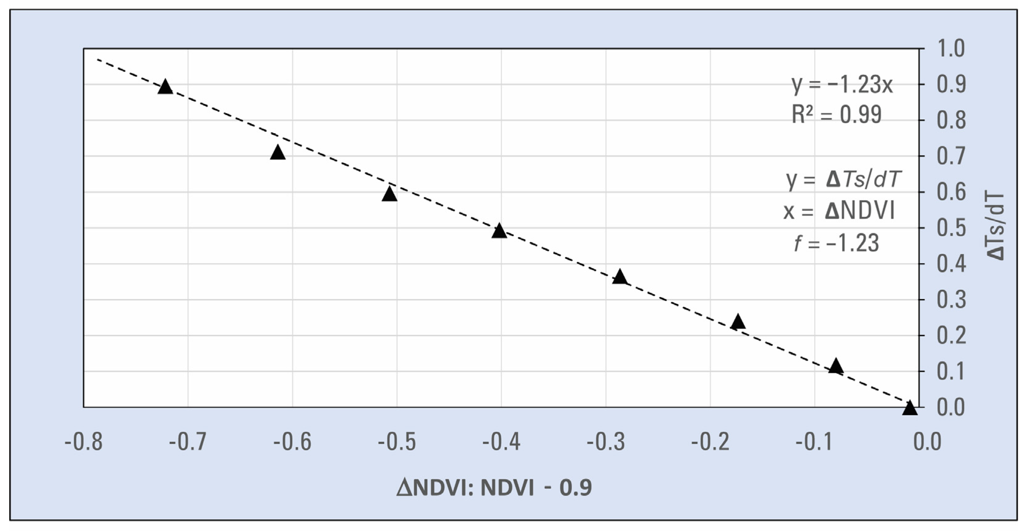
2.2.4. Calculation of c Factor

Within FANO, the wet-bulb Tc^* is only determined at a coarse resolution (5 km grid or larger) and thus the 1 km air temperature is used to disaggregate and create the final Tc at a 1 km resolution using a similar c factor calculation as in previous publications (e.g., Senay et al. [15,18]. The disaggregation is generally useful in complex topography where the Tc may show a substantial spatial variation within a 5 km grid.

$$c=\frac{T{c}^{*}}{T{a}^{*}}$$

(9)

where c is the factor that relates wet-bulb reference surface temperature with air temperature; Ta^* is the spatially averaged (5 km) maximum daily air temperature (climatology); and Tc^* is the predicted wet-bulb reference surface temperature as defined earlier at 5 km.

$$Tc=c·Ta$$

(10)

where Tc is the final wet-bulb reference surface temperature at 1 km; and Ta is the 1 km maximum daily air temperature (climatology) that is used to disaggregate Tc^* using the c factor. Note the absence of * in Equation (10), indicating the absence of large area averaging.

2.3. Model Performance Evaluation

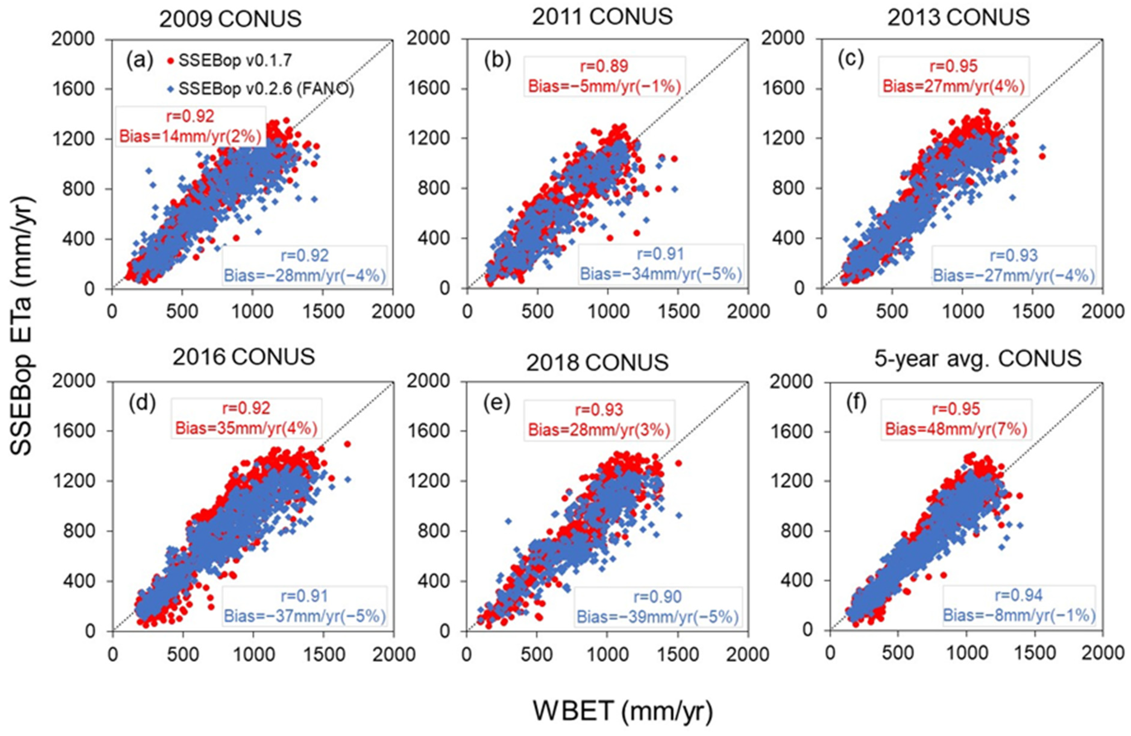
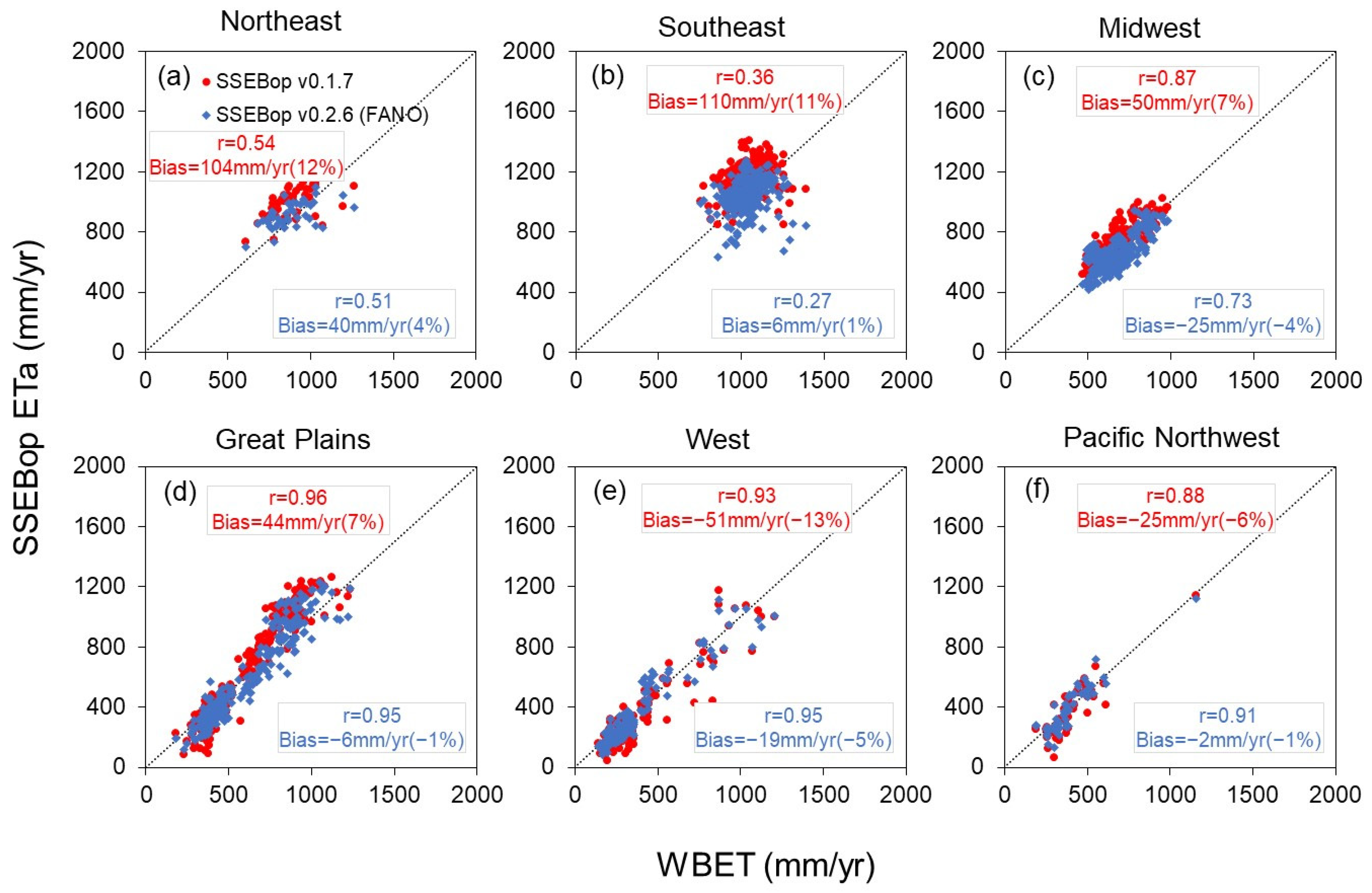
2.3.1. Water Balance Evaluation

An independent water balance ETa (WBET) generated at the Hydrological Unit Code (HUC) sub-basin (HUC8) scale [28] was compared with SSEBop ETa at the water-year (1 October–30 September) timestep. The water-year scale minimizes the effect of unaccounted storage changes that are important at shorter time scales. The water-year, hereafter named as annual WBET for HUC8s, was computed as:

$$WBET=P-Q-\Delta S$$

(11)

where P, Q, and ΔS are annual precipitation, runoff, and storage change, respectively, at HUC8 sub-basins.

For the WBET estimation at the HUC8 scale, P and Q data were used. Monthly P at 4 km spatial resolution was obtained from the Parameter-elevation Regressions on Independent Slopes Model (PRISM) [29]. Monthly P was aggregated to annual totals to obtain a single basin-average value for each HUC8. Annual Q for HUC8s was obtained from the U.S. Geological Survey (USGS) WaterWatch (https://waterwatch.usgs.gov/, accessed on 20 June 2022). These annual Q values (non-spatial) at the HUC8 scale are generated from historical flow observations at the USGS stream gages, drainage basin boundaries of the stream gages, and the HUC8 boundaries [30]. Following previous studies [16,31,32], the annual storage change (ΔS) was assumed to be negligible (0.0) during the study period.

Following similar assumptions and techniques reported in the literature [16,33,34], several filters were applied to exclude HUC8s where the water balance is not expected to close (WBET ≠ P − Q). The HUC8s with Q/P > 0.40 [16], HUC8s with WBET greater than potential ET, and HUC8s with SSEBop ETa greater than precipitation (heavily irrigated HUC8s that the ETa from WBET does not consider) were excluded.

The annual total ETa from SSEBop v0.1.7 [16,35] and SSEBop v0.2.6 (FANO) were compared with WBET for average and individual years during the 5-year (2009, 2011, 2013, 2016, 2018) period. These years were selected to include both wet (2016), dry (2011), and normal (2009, 2013, 2018) years. The 5-year average ETa comparisons were also grouped across six different hydro-climatic regions of the CONUS to evaluate the performance of the FANO across the regions. The correlation coefficient (r), bias, MAE (mean absolute error), and RMSE (root mean square error) were applied for statistical analysis.

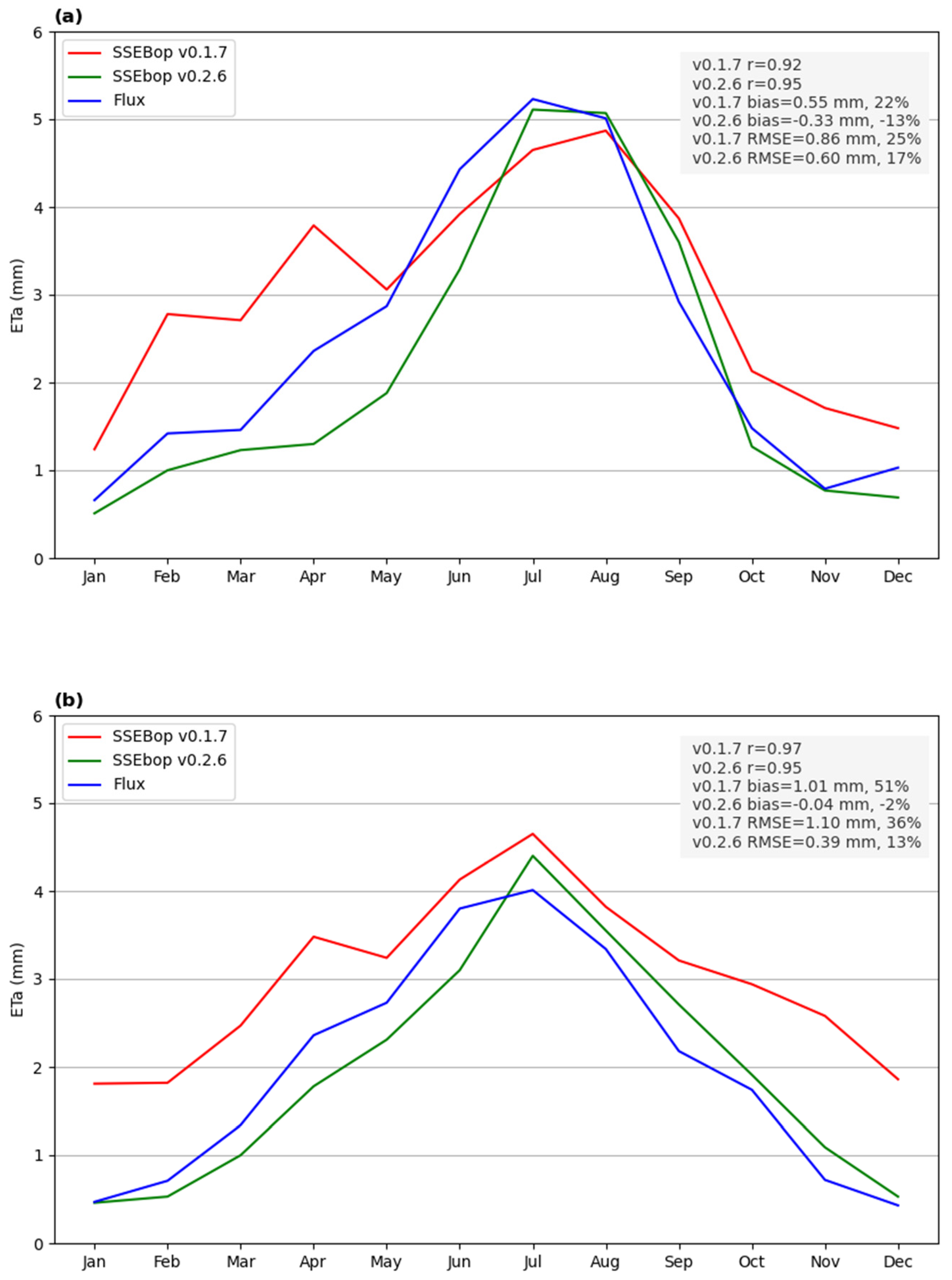
2.3.2. Evaluation with Flux Tower Data

Following previous studies such as Senay et al. [35] and Senay et al. [16], the accuracy of the SSEBop ETa using the new FANO implementation was evaluated with eddy covariance (EC) flux tower data from the Ameriflux network (https://ameriflux.lbl.gov/, accessed on 15 March 2022). For this evaluation, 23 Ameriflux EC towers were selected in a northeast-southwest swath across the central United States for three consecutive years from each tower for the 2008–2019 period (Figure 1).

Unlike in Senay et al. [16], rather than using the FLUXNET2015 dataset, which ends before the year 2015, we used the flux-data-qaqc Python package for Energy Balance Closure and Post-Processing of the Ameriflux EC data [36]. This Python package quantifies and standardizes the gap-filling and energy balance closure more efficiently and more uniformly than previous methods using an Energy Balance Ratio approach. The flux-data-qaqc package processes daily actual ET in mm/day, which was matched with the corresponding overpass SSEBop Landsat ETa and the comparison was conducted at the overpass level for a three-year period at each tower location.

The SSEBop ET Fraction (ETf) was calculated for all overpass imagery with less than 60% cloud cover for a corresponding three-year period at each tower location. The ETf was calculated twice: (1) for the previous, high NDVI-based c factor version (v0.1.7) described in Senay et al. [16,18], and (2) for the newly developed FANO parameterization of c factor (v0.2.6) described above. To calculate actual ET from the SSEBop ET fraction, two versions of the alfalfa-reference ET (ETr) from the Gridmet dataset were used to calculate ETa: (1) a climatology daily mean of 1981–2010 Gridmet ETr, and (2) using the corresponding original annual (yearly) Gridmet ETr for each overpass date. This resulted in four versions (two model versions by two reference ETr) of SSEBop ETa at the overpass level that were compared to the ETa derived from the EC tower data.

The gridded Gridmet ETr was also compared to a pointed-based reference ETr from EC towers weather stations to determine a potential bias of Gridmet against station data. Key input variables from the EC tower weather station were fed into the Reference Evapotranspiration Calculator (Ref-ET) software program from the University of Idaho that calculated alfalfa-reference ET using the ASCE Standardized Penman Monteith Reference Equation (https://www.uidaho.edu/cals/kimberly-research-and-extension-center/research/water-resources/ref-et-software, accessed on 14 May 2022). Both the climatology and annual daily values of Gridmet ETr at each tower location were compared to the ETr derived from the Ref-ET software from the EC tower for the matching years of the EC tower validation study. No scaling factors were used for the climatology or annual Gridmet ETr in order to determine the bias and error in ETr from the model-assimilated gridded Gridmet dataset against the station-based EC tower ETr.

Although the EC towers are not well-distributed across space or landcover, the overall aggregate statistics, including r, RMSE, and percent bias, from all cropland and grassland EC Towers (n ≥ 5 EC Towers) were calculated as well as the overall aggregate statistics from all tower locations and overpass dates (n = 1115, representing station-overpass data points). Monthly averages of cropland and grassland overpass ETa values were used to construct and compare seasonal patterns of ETa from model and EC tower datasets.

2.4. Computing Platforms

2.4.1. Google Earth Engine Implementation of SSEBop

Production of SSEBop ET data in this study was completed using the Google Earth Engine (GEE) platform [37] for the generation of ETf at the EC tower sites and ETa (annual water year) used for the nationwide WBET analysis. We used the open-access SSEBop-FANO v0.2.6 Python implementation available at https://github.com/Open-ET/openet-ssebop (accessed on 21 April 2022) and featuring model configuration setup for the FANO parameters as discussed in Section 2.2.3. To achieve time-integrated annual ETa, we performed routine aggregation calculations, as followed in Senay et al. [16], for linear interpolation of daily ETf from Landsat satellite overpass. Using daily ETr, we produced daily total ETa and summed for our time periods of interest: 1 October–30 September water years for 2009, 2011, 2013, 2016, and 2018.

By using GEE developer tools during our model modernization efforts, our progress and algorithms matured through iterative method refinements that led to research and development insights for Landsat ET processing that were then directly realized within the USGS Earth Resources Observation and Science (EROS) Center Science Processing Architecture ESPA programming phase of the latest USGS global Level-3 ETa science products.

2.4.2. USGS On-Demand Overpass SSEBop ETa

The SSEBop FANO v0.2.6 ETa described in this paper and processed in GEE has also been implemented as a Landsat Level-3 Provisional Science Product that was made publicly available for on-demand processing through the USGS (EROS) ESPA environment (https://espa.cr.usgs.gov/, accessed on 4 August 2022) in August 2022. This interface provides the public with the ability to order SSEBop ETa identical to that described in this paper for any Landsat Collection 2 (C2) image from Landsat 4–9 satellites for any location on the globe dating back to 1982. ESPA also offers an Application Programming Interface (API) for programmatic ordering and downloading of Landsat C2 ETa (https://www.usgs.gov/media/files/eros-science-processing-architecture-demand-interface-user-guide, accessed on 4 August 2022).

In order to process a C2 ETa for Landsat thermal-infrared acquisitions (Landsat 4–9), ESPA will require the Level-2 Science Product (L2SP) identifier for that scene, which includes both Surface Reflectance and Surface Temperature information. Once the L2SP scene is retrieved from the Landsat archive, relevant surface reflectance and surface temperature bands are extracted and then the SSEBop model is run using the auxiliary data described in Section 2.1 (https://www.usgs.gov/media/files/landsat-4-9-collection-2-level-3-provisional-actual-evapotranspiration-algorithm, accessed on 4 August 2022). Landsat Collection 2 archive also includes Level-2 Surface Reflectance (L2SR) scenes that cannot be processed to ETa due to lack of surface temperature information; these scenes can occur over certain areas such as the Aleutian Islands, the Antarctic, or other small islands where the inputs needed for surface temperature are unavailable. The characteristics of the on-demand Landsat C2 L3 ETa is documented in the product guide (https://www.usgs.gov/media/files/landsat-4-9-collection-2-level-3-provisional-actual-evapotranspiration-product-guide, accessed on 4 August 2022) as well as the Landsat Mission Website (https://www.usgs.gov/landsat-missions/landsat-collection-2-provisional-actual-evapotranspiration-science-product, accessed on 4 August 2022). The processing runtime for any individual Landsat scene is typically around two minutes and many scenes can be run in parallel using Python and Linux environments.

The SSEBop ETa generated from ESPA and that generated in GEE for this study share more than 99% similarity on a per-scene basis as of v0.2.6 (FANO implementation). The GEE-based SSEBop evaluation results described in this study can be extended to the ESPA version of SSEBop as the two versions are nearly identical. The ESPA SSEBop ETa is available at a global extent and four sample scenes are provided in Section 3 including a summary of ETa by landcover type. Landcover types used to evaluate ESPA products were downloaded from the MODIS (Moderate Resolution Imaging Spectroradiometer) Land Cover Type L3 500 m Grid (MCD12Q1v006).

3. Results

3.1. Water Balance Evaluation

Figure 6 demonstrates the map of annual ETa calculated from a 5-year median using the SSEBop FANO model. The median was chosen for Figure 6 (small number of years) while the average was used for the statistical comparison against WBET. The CONUS-wide HUC8 annual ETa comparison for each water year and the 5-year (2009, 2011, 2013, 2016, and 2018) average is shown in Figure 7. The overall results indicate the improved performance of SSEBop v0.2.6 (FANO) over the SSEBop v0.1.7. Bias is reduced from 48 mm/year (7%) with SSEBop v0.1.7 to −8 mm/year (−1%) with SSEBop v0.2.6 (FANO) for 5-year average at CONUS scale (

Table 3. Summary of HUC8 ETa comparison between SSEBop v0.1.7 and SSEBop v0.2.6 (FANO) with water balance (WBET) for 5-year average (5-y avg.) and individual years. The Pearson correlation coefficient (r) shows the degree of association between the two versions of SSEBop and WBET for the six regions and CONUS.

Region +	Water Year	WBET mm/yr	n1	r (−)		Bias, mm/yr (%)		MAE, mm/yr (%)		RMSE, mm/yr (%)
				SSEBop v0.1.7	SSEBop v0.2.6 (FANO)	SSEBop v0.1.7	SSEBop v0.2.6 (FANO)	SSEBop v0.1.7	SSEBop v0.2.6 (FANO)	SSEBop v0.1.7	SSEBop v0.2.6 (FANO)
NE	5-y avg.	883	44	0.54	0.51	104 (12)	40 (4)	141 (16)	97 (11)	154 (17)	123 (14)
SE	5-y avg.	1033	246	0.36	0.27	110 (11)	6 (1)	134 (13)	95 (9)	160 (16)	129 (12)
MW	5-y avg.	672	279	0.87	0.73	50 (7)	−25 (−4)	59 (9)	73 (11)	76 (11)	87 (13)
GP	5-y avg.	626	242	0.96	0.95	44 (7)	−6 (−1)	103 (16)	78 (13)	128 (20)	99 (16)
W	5-y avg.	383	136	0.93	0.95	−51 (−13)	−19 (−5)	79 (21)	63 (17)	104 (27)	80 (21)
P NW	5-y avg.	398	53	0.88	0.91	−25 (−6)	−2 (−1)	68 (17)	52 (13)	86 (22)	68 (17)
CONUS	2009	702	1000	0.92	0.92	14 (2)	−28 (−4)	101 (14)	94 (13)	128 (18)	122 (17)
	2011	640	751	0.89	0.91	−5 (−1)	−34 (−5)	108 (17)	100 (16)	138 (22)	126 (20)
	2013	684	946	0.95	0.93	27 (4)	−27 (−4)	98 (14)	87 (13)	128 (19)	113 (16)
	2016	780	1024	0.92	0.91	35 (4)	−37 (−5)	120 (15)	106 (14)	150 (19)	134 (17)
	2018	805	773	0.93	0.90	28 (3)	−39 (−5)	105 (13)	109 (13)	133 (17)	139 (17)
	5-y avg.	705	1000	0.95	0.94	48 (7)	−8 (−1)	95 (13)	78 (11)	122 (17)	104 (14)

¹: n = number of HUC8s for ETa comparison between SSEBop (identical HUCs on two versions) and WBET. ⁺: NE = Northeast; SE: Southeast; MW: Midwest; GP = Great Plains; W: West; P NW = Pacific Northwest.

). Similarly, MAE reduced from 95 mm/yr (13%) to 78 mm/yr (11%) and RMSE from 122 mm/yr (17%) to 104 mm/yr (14%). The r values are above 0.93 for both versions of SSEBop at the CONUS scale. Overall, the SSEBop v0.2.6 (FANO) tends to lower the ETa positive bias from SSEBop v0.1.7, resulting in a slight negative bias at the 5-year average (Table 3).

The individual water-year comparison also shows a negative bias from SSEBop v0.2.6 (FANO), compared to the positive bias from SSEBop v0.1.7 (except for water year 2009). Both negative and positive biases from both versions of SSEBop are within ±5% for all water years (Table 3). SSEBop v0.2.6 (FANO) showed negative bias for both dry (2011) and wet (2016) water years, whereas SSEBop v0.1.7 showed positive and negative biases for the wet and dry water years, respectively. The MAE and RMSE are lower for SSEBop v0.2.6 (FANO) compared to SSEBop v0.1.7 for all water years except water year 2018. The r values are comparable on both versions of SSEBop at ≥0.89 for all water-years.

The regional HUC8 ETa comparison of SSEBop v0.1.7 and SSEBop v0.2.6 (FANO) with WBET is shown in Figure 8. Overall results indicate a better performance of SSEBop v0.2.6 (FANO) over SSEBop v0.1.7. Bias is reduced from SSEBop v0.2.6 (FANO) at all regions, resulting in within ±5% (Table 3). MAE and RSME are also lower from SSEBop v0.2.6 (FANO) at all regions except the Midwest region. The SSEBop v0.1.7 shows positive bias at the Northeast and Southeast regions (>10%), but these magnitudes are lowered by SSEBop v0.2.6 (FANO) (<5%). Similarly, the high negative bias by SSEBop v0.1.7 at the West and Pacific Northwest regions (≥6%) are lowered by SSEBop v0.2.6 (FANO) (≤5%). The overall pattern of positive bias at the eastern regions (Northeast and Southeast) and negative bias at the western regions (West and Pacific Northwest) remain similar from both versions of SSEBop. However, the positive bias from SSEBop v0.1.7 at the Midwest and Great Plains regions show with a smaller negative bias with SSEBop v0.2.6 (FANO).

3.2. EC Tower Evaluation

The evaluation results of SSEBop ETa against ETa from the EC flux towers show that the FANO implementation brings a positive improvement in accuracy.

In relation to climatology Gridmet, the annual Gridmet shows a higher bias and RMSE, but with a stronger correlation against the EC Tower ETr. Due to a potential smoothing effect of the climatology, especially over the higher values during drier years, the climatology ETr shows little bias (−0.2% versus 15.6%) (

Table 4. Flux Tower Alfalfa Reference Evapotranspiration (ETr) comparison with Gridmet Alfalfa Reference Evapotranspiration for 23 Ameriflux eddy covariance (EC) Towers. ETr values in the first two columns refer to the two Gridmet daily datasets used in the comparison: Climatology 1981–2010 average ETr and annual ETr (for the same years used in the ETa validation). Values are the average of all overpass days from all towers (n = 925) with the standard deviation (STD) given in brackets.

Gridmet Version	Tower ETr (mm) [STD]	GMET ETr (mm) [STD]	Bias (mm) [%]	RMSE (mm) [%]	r (−)
Climatology *	5.84 [2.98]	5.83 [2.24]	−0.01 [−0.2%]	1.86 [32%]	0.78
Annual	5.84 [2.98]	6.76 [3.06]	0.91 [15.6%]	1.98 [34%]	0.83

*: Flux ETr does not have climatology. The annual station ETr is compared to the climatology and annual (yearly) Gridmet ETr.

). Therefore, while a climatology Gridmet may not require an adjustment, the annual ETr appears to require an adjustment of about 15%, which is comparable to the findings of Blankenau et al. [39] who reported a bias range of 12% to 31% across CONUS. Bawa et al. [40] also used a correction coefficient of 0.85 to account for the higher bias in Gridmet during the generation of ETa over the Missouri River Basin.

For comparison with the EC Tower ETa, SSEBop used both Gridmet ETr datasets: climatology and annual, scaled and unscaled. The closest comparisons with the EC Tower data came from the SSEBop ETa using the climatology without any scaling and the annual ETr scaled down by 15%. However, SSEBop using either a climatology or annual ETr showed measurable improvement in accuracy against EC tower ETa with v0.2.6 (FANO) implementation as compared to the previous version of SSEBop ETa [16]. When using climatology ETr, SSEBop ETa improved the overall bias from the EC Towers from 39.2% in v0.1.7 down to only 3.0% above the tower in v0.2.6 (FANO) along with a reduction in RMSE from 1.76 mm down to 1.36 mm (

Table 5. Comparison between SSEBop and flux tower ETa using two model versions (v0.1.7 and v0.2.6) and two reference ET sources (annual and climatology Gridmet) over 23 Ameriflux eddy covariance (EC) towers. Top section compares the Gridmet climatology 1981–2010 ETr and the bottom section compares the Gridmet annual ETr (for the same years used in the ETa validation) on satellite overpass days. ETa values for the towers and SSEBop ETa are the average of all overpass days from all towers (n = 1115) with the standard deviation (STD) given in brackets.

SSEBop Version	Gridmet Version	Tower ETa (mm) [STD]	SSEBop ETa (mm) [STD]	Bias (mm)	RMSE (mm)	r (−)	Percent Bias (%)
v0.1.7	Climatology *	2.32 [2]	3.23 [1.78]	0.91	1.76	0.69	39.2%
v0.2.6	Climatology *	2.32 [2]	2.39 [1.94]	0.08	1.36	0.76	3.0%
v0.1.7	Annual **	2.32 [2]	3.2 [1.96]	0.88	1.88	0.65	37.9%
v0.2.6	Annual **	2.32 [2]	2.4 [2.06]	0.08	1.47	0.74	3.4%

*: Flux ETa does not have climatology. The annual station ETa is compared to the climatology and annual Gridmet ETa. **: the annual Gridmet ETa was scaled down using a factor of 0.85 to account for known bias.

). It is important to note that part of the SSEBop ETa RMSE could be attributed to the Gridmet-related RMSE, which showed an RMSE of 1.86 mm when compared to station ETr (Table 4). This indicates the importance of accounting for the effect of ETr when trying to improve model performance.

SSEBop also showed an improvement in correlation with the EC Tower ETa from r = 0.69 in v0.1.7 up to r = 0.76 with v0.2.6 (FANO) when pooling all stations across landcover types (Table 5). Similarly, when using the annual Gridmet ETr scaled by a factor of 0.85 (equivalent to a 15% reduction in magnitude), SSEBop ETa improved in performance from v0.1.7 [16] to v0.2.6 (FANO). The reduction in overall bias was almost identical, dropping from >37.0% with v0.1.7 to <4% above the EC towers with v0.2.6 regardless of the type of ETr (Table 5). Similarly, the RMSE reduces from 1.88 mm in v0.1.7 down to 1.47 mm in v0.2.6 (FANO) using the annual ETr. The correlation between the EC Tower ETa and SSEBop ETa also improves from r = 0.69 and r = 0.65 for v0.1.7 using the climatology and annual ETr, respectively, to r = 0.76 and r = 0.74 with v0.2.6 (FANO), which corresponds to approximately a 10% increase in correlation using the new FANO implementation (Table 5).

The number of EC towers was insufficient to summarize the results by different landcover as some landcover types only included a single tower, but cropland and grassland sites had at least five tower sites and at least 295 or more data points for comparison.

Table 6. Overpass actual ET (ETa) comparison between SSEBop and flux tower categorized by landcover (as reported by Ameriflux). SSEBop was forced with the climatology Gridmet 1981–2010 ETr without any scaling factor.

Landcover	SSEBop Version	Count	Average Tower ETa (mm) [STD]	Average SSEBop ETa (mm) [STD]	Bias (mm)	RMSE (mm)	r (−)	Percent Bias (%)
Cropland	v0.1.7	295	3.13 [2.26]	3.47 [1.92]	0.34	1.48	0.77	11%
Cropland	v0.2.6	295	3.13 [2.26]	2.91 [2.22]	−0.22	1.21	0.86	−7%
Grassland	v0.1.7	400	2.1 [1.97]	3.08 [1.63]	0.98	1.88	0.61	47%
Grassland	v0.2.6	400	2.1 [1.97]	2.06 [1.64]	−0.04	1.35	0.73	−2%

shows the summary accuracy statistics of these two landcover types. For the cropland sites (n = 8), the improvement in SSEBop accuracy from v0.1.7 to v0.2.6 (FANO) was measurable although less than the overall averages (23 sites) shown above in Table 5. For cropland sites, SSEBop improved from v0.1.7 to v0.2.6 (FANO) in correlation where the r improved from 0.77 to 0.86; the RMSE improved from 1.48 mm to 1.21 mm, and in bias, where the percent bias dropped from 11% to −7%, although the bias for both v0.1.7 and v0.2.6 (FANO) stayed within 15% of the tower. The grassland sites (n = 6) also showed a clear improvement in accuracy of SSEBop ETa between v0.1.7 and v0.2.6 (FANO) where the percent bias dropped from 47% in v0.1.7 down to only −2% in v0.2.6. The correlation improved from r = 0.61 in v0.1.7 up to r = 0.73 in v0.2.6 (FANO) and the RMSE error reduced from 1.88 mm to 1.35 mm. Although both cropland and grassland had improvements in correlation, error, and magnitude from v0.1.7 SSEBop ETa to v0.2.6 (FANO), the improvements on grassland are more substantial, which strengthens the FANO implementation on a wider scale. It is important to note that these are daily scale comparisons and the RMSE and correlation are expected to improve with larger aggregation periods such as monthly and seasonal times scales.

Figure 9 displays the seasonality of monthly averages of SSEBop ETa (two model versions) and EC Tower ETa for both cropland and grassland sites. The blue line in Figure 9a (flux) shows the average ETa from the eight cropland sites for each month from the EC towers. The red line (SSEBop v0.1.7) shows the SSEBop ETa from v0.1.7, which generally matches the EC towers during the summer months, with some underestimation, but greatly exceeds the EC Towers during the winter and early spring months and again after the harvest in the fall months (Figure 9a). The green line (SSEBop FANO v0.2.6), on the other hand, does not show the same overestimation in the winter or shoulder months (actually shows underestimation) and also shows much higher correlation with the seasonal pattern of ETa from the EC towers (Figure 9a). The improvement in seasonal pattern of ETa for SSEBop v0.2.6 (FANO) as opposed to SSEBop v0.1.7 is well illustrated. However, the spring season underestimation by v0.2.6 over cropland sites requires further investigation.

The seasonal pattern of SSEBop ETa is similarly improved for grassland sites (n = 6) with even higher agreement between EC tower ETa and SSEBop ETa with FANO (Figure 9b). SSEBop v0.1.7 shows higher biases on a monthly level compared to the EC tower ETa for most of the year with biases lessened in the peak summer months. SSEBop v0.2.6 (FANO), on the other hand, shows higher agreement with the flux tower ETa, only slightly underestimating the towers in the spring months and overestimating in the peak summer and fall months. The accuracy metrics shown in Figure 9 at monthly time scale are much improved compared to that presented in Table 6 (daily) due to the spatiotemporal averaging effect on random errors except the bias, which remains more comparable to daily statistics as expected. The bias differences between the monthly (Figure 9) and the daily (Table 6) can be attributed to different sample size across the months, with fewer stations in the winter compared to summer season. For example, using SSEBop FANO accuracy improvements from daily to monthly for cropland show with r (0.86 versus 0.95) and RMSE (1.21 versus 0.60 mm/day) and for grassland with r (0.73 versus 0.95) and RMSE (1.35 versus 0.39 mm/day). The accuracy metrics for daily (Table 6) and monthly (Figure 9) are comparable to metrics for remote sensing ET models reported by OpenET [41].

3.3. On-Demand SSEBop Evapotranspiration

The GEE Python-based SSEBop v0.2.6 (FANO) code is available for download at https://github.com/Open-ET/openet-ssebop (accessed on 21 April 2022). The global SSEBop ETa product from the same version is available on-demand for each Landsat scene from the USGS EROS ESPA environment (https://espa.cr.usgs.gov/, accessed on 4 August 2022).

Figure 10 displays a sample of four Landsat SSEBop ETa images downloaded from ESPA for locations in (Figure 10a) the Central Valley of California, (Figure 10b) near the Nile River Delta in Egypt, (Figure 10c) in the state of Bahia, Brazil, and (Figure 10d) near Nanjing, China, in the Yangtze River Delta. This represents the ETa expressed over the landscape for an individual day when there is a Landsat observation, with arbitrary dates chosen for each scene. Landcover-based spatially averaged SSEBop ETa shows the relative amounts of ETa by landcover type with croplands using around 3.8 mm for a mid-season date in California; 1.5 mm of ETa for a late-season date in Bahia, Brazil; 2.6 mm of ETa for a late-season date in Egypt; and 4.3 mm of ETa for a mid-season date in Nanjing, China (Figure 11). ESPA SSEBop ETa provides a prediction of SSEBop ETa (with the new FANO implementation) for every Landsat observation for any given area. Users can download overpass-level SSEBop ETa from ESPA and using simple linear interpolation tools can interpolate and aggregate to a monthly ETa with an algorithm of their choice.

4. Discussion

4.1. WBET Evaluation

Comparisons of annual ETa for the 5-year average, each water year, and across six different regions show a good agreement between both versions of SSEBop and WBET. The performance of SSEBop varied with a distinct regional difference with positive bias at the eastern regions (Northeast and Southeast) with higher ETa rates and negative bias at the western regions (West and Pacific Northwest) with lower ETa rates. The larger positive biases at the eastern regions and larger negative bias at the western regions by SSEBop v0.1.7 are lowered by SSEBop v0.2.6 (FANO), reflecting the improved performance. The percent bias from SSEBop v0.2.6 (FANO) is within ±5% for each water year and 5-year average, compared to ± 13% from the SSEBop v0.1.7 (

Table 7. Summary of non-matching (different n values) HUC8 ETa comparison between SSEBop v0.1.7 and SSEBop v0.2.6 (FANO) with water balance (WBET) for CONUS and the six regions. Bias, MAE, and RMSE are yearly magnitudes (mm/year) with percent of the 5-year average shown in brackets (%).

Statistics	CONUS		Northeast		Southeast		Midwest		Great Plains		West	Pacific Northwest
	v0.2.6	v0.1.7	v0.2.6	v0.1.7	v0.2.6)	v0.1.7	v0.2.6	v0.1.7	v0.2.6	v0.1.7	v0.2.6	v0.1.7	v0.2.6	v0.1.7
n	1222	1079	44	44	261	247	285	281	415	264	161	184	56	59
r	0.94	0.96	0.51	0.54	0.24	0.34	0.74	0.87	0.95	0.96	0.94	0.92	0.90	0.84
Bias, mm (%)	−7 (−1)	43 (6)	40 (4)	104 (12)	14 (1)	112 (11)	−24 (−4)	50 (8)	−12 (−2)	39 (6)	−15 (−4)	−52 (−14)	4 (1)	−10 (−3)
MAE, mm (%)	74 (11)	94 (14)	97 (11)	141 (16)	98 (9)	135 (13)	72 (11)	60 (9)	66 (11)	99 (16)	60 (16)	77 (20)	55 (14)	74 (19)
RMSE, mm (%)	97 (14)	121 (18)	123 (14)	154 (17)	130 (13)	163 (16)	86 (13)	77 (11)	87 (14)	124 (20)	78 (21)	100 (27)	72 (18)	91 (23)

). These biases are similar to the range of errors reported in the previous studies [16,33,34] and within the expected bias range of 10–20% from remote sensing-based energy balance algorithms [42].

For the individual water-year comparison, there are a few HUC8s where SSEBop v0.2.6 (FANO) showed a substantial negative bias in comparison to WBET (e.g., Figure 7b). Such negative biases are consistent for all water years except the wet water year 2016 (Figure 7d). These HUC8s are in the West region (California) and had runoff (Q) value of zero (0.0), resulting in higher WBET, which in turn creates a substantial negative bias by SSEBop v0.2.6 (FANO).

The filters applied to HUC8s where the water balance is not expected to close resulted in the exclusion of about 50% of the total 2,121 HUC8s in the CONUS (Table 3). Upon applying the filters (Section 2.3.1) for the 5-year average comparison individually, SSEBop v0.1.7 resulted in 1079 comparable HUC8s, whereas SSEBop v0.2.6 (FANO) resulted a larger (13% more) number of comparable HUC8s at 1222 (Figure 1). The increase in WBET-qualified HUC8s is mostly in the Great Plains region, with an increase of 415 HUC8s with SSEBop v0.2.6 (FANO) compared to 264 HUC8s with SSEBop v0.1.7. However, on a one-to-one comparison of the two versions of SSEBop for the CONUS-scale comparison, there are only 1000 identical HUC8s that are comparable between both versions of SSEBop and WBET (Table 3).

The independent (non-matching HUCs between v0.1.7 and v0.2.6) evaluation (1222 HUC8s) of SSEBop v0.2.6 (FANO) showed comparable performance to the one-to-one comparison (1000 HUC8s) both at the CONUS and regional scales. The bias, MAE, and RMSE are −7 mm/year (−1%), 74 mm/year (11%), and 97 mm/year (14%), respectively for the 5-year average at CONUS scale (Table 7). For the regional scale, the percent bias, percent MAE, and percent RMSE are within ±4%, 16%, and 21%, respectively. In the Great Plains region, where the number of comparable HUC8s increased (Figure 1), SSEBop v0.2.6 (FANO) decreased the percent bias, percent MAE, and percent RMSE from 6% to −2%, 16% to 11%, and 20% to 14%, respectively, compared to SSEBop v0.1.7 (Table 7). The r values are ≥0.90 for CONUS scale and ≥0.73 for regional scale comparisons, except the Northeast and Southeast regions (Table 7). The ETa values for the Northeast and Southeast regions are clustered and lack a dynamic range (Figure 8a,b) compared to other regions (Figure 8c–f), resulting in relatively lower r values. However, the model captures the average values accurately as demonstrated by the bias, MAE, and RMSE.

4.2. FANO Constant

The linear relation between crop coefficient (Kc) (comparable to ETf, when water is non-limiting) and NDVI has been reported by several researchers [43,44,45]. Allen et al. [46] summarized the degree of the linear relation with a 1.25 proportionality constant when Kc is expressed as the fraction of the alfalfa-based reference ET, i.e., Kc = 1.25 * NDVI. It important to note the independent formulation of Kc and ETf in that Kc is estimated as the ratio of actual ET to reference ET whereas ETf is estimated using Equation (2) from land surface temperature using the principle of satellite psychrometry.

In related studies, Ruimy and Saugier [47] also established a similar coefficient of 1.25 in relating the fraction of incoming photosynthetically active radiation (fPAR) and NDVI in their parametric equation for the estimation of terrestrial net primary production. Palmer and Yunusa [48] used a linear formulation to estimate actual evapotranspiration and biomass from fPAR, which can be derived from NDVI using a linear assumption [49].

Thus, the Senay Approximation in Equation (3) and the FANO constant of 1.25 can be related to empirically established foundations in the use of NDVI for estimating related properties such as primary production or ET. In this study, the FANO formulation uses different sets of parameters (dT, NDVI, and Ts) to determine a theoretical wet-bulb reference temperature using an identical constant of 1.25, which is labeled as a FANO constant. Although the FANO constant of 1.25 appears to be a reasonable magnitude for large applications, more localized uses could benefit from a calibrated value specific to the study region.

4.3. Climatology vs. Annual Gridmet Reference ET

One of the findings in this study is that the use of a climatology ETr produces a comparable ETa as using an annual (yearly) ETr, particularly at longer time scales. Using station-based annual ETr as the truth, while the correlation coefficient was slightly higher with the annual (r = 0.83) as compared to the climatology (r = 0.78), the bias (−0.2% versus 15.6%) and RMSE (32% versus 34%) were better with the climatology ETr compared to the annual ETr (Table 4). However, the differences were dampened at the actual ETa level (Table 5), highlighting the importance of the land surface temperature in controlling the spatiotemporal variability of ETa. This reinforces the reliability of climatology ETr, especially for operational applications as used by the global ESPA-based SSEBop ETa. Additionally, it validates the use of a bias correction factor for the annual Gridmet ETr.

4.4. Challenges and Limitations

Although the FANO formulation for Tc determination improves the operational estimation of ETa in sparsely vegetated surfaces such as grasslands where high NDVI are difficult to find on the earlier v0.1.7 parameterization, challenges remain on the potential effect of using a constant dT (climatology) in Equation (3) with v0.2.6. However, because dT and NDVI are linked in the FANO parameterization (Equation (8)), the role of high or low dT on ETf or ETa is different depending on whether the Ts of a pixel is higher or lower than Ts^*. Future research could look into the sensitivity of the dT parameter and its effect on the final ETa product.

There is a unique challenge with low NDVI landscapes in that the Tc is extrapolated too far using the linear equation. The low NDVI challenge is similar to one reported by Ruimy and Saugier [47] where they expected the greatest errors in using a constant linear NDVI relationship to occur over areas with low NDVI (i.e., areas with small vegetation cover). According to Huete [50], errors caused by soil effects amount to about 10%. In addition to NDVI from sparse vegetation, water bodies are also modeled with maximum ET rates (Table 2) without taking into account seasonal heat storage changes [51]. Thus, modeled ETa from deep waterbodies may not be reliable at a monthly rate but could provide a reasonable estimate at annual time scales due to a seasonal shift in heat storage and release.

The assumption of homogeneous hydroclimatic region with the 5 km grid for the FANO implementation may not be realistic over highly complex terrain where large elevation changes could exist within short distances. This becomes more challenging when the high resolution (1 km) air temperature is not well represented to disaggregate the c factor from 5 km to 1 km (Equation (10)). Such problems tend to be exaggerated in arid areas with isolated mountains with poor quality air temperature datasets with an overall effect of overestimating ET over high elevation outcrops in an otherwise flat terrain.

5. Conclusions

The study outlined the formulation of a new FANO parameterization scheme for the determination of the wet-bulb reference temperature in the SSEBop model and evaluated the performance of the updated model using EC tower and water balance-based ET estimates.

The FANO parameterization proved superior in model performance and operational implementation. FANO allowed the establishment of the cold boundary condition (wet-bulb) regardless of vegetation cover density, improving the performance and operational implementation of the model in sparsely vegetated landscapes and outside of the main growing season.

Accuracy metrics improved substantially for grassland landcover, reducing obvious over-estimation bias (47% versus −2%) while maintaining a comparable level of accuracy over croplands (11% versus −7%), which was already performing reasonably well in the previous version. CONUS-wide basin-scale comparison with annual water balance ET shows an improvement (reduced under-estimation) on the low end (<400 mm/year) and high end (>800 mm/year, reduced over-estimation) while maintaining a comparable result in the mid-ranges with an overall accuracy within 5%. Furthermore, visual inspection of annual ET maps shows an improved spatial pattern by eliminating artifacts observed in the earlier version.

A comparison of climatology versus annual ETr with station-based ETr showed that while the correlation of the annual ETr was slightly better than the climatology ETr, bias and RMSE errors are better with climatology ETr. More importantly, the actual ETa using the SSEBop model produced comparable results using either climatology or annual gridded ETr. This indicates the use of climatology gridded ETr is valid for large scale applications.

Continued evaluation and bias corrections are necessary to improve the absolute magnitude of ET estimation for localized water budget applications. The SSEBop FANO parameterization has demonstrated the capability to capture the spatiotemporal dynamics of global landscape ETa.

Overpass daily ETa can be ordered at https://espa.cr.usgs.gov/ (accessed on 4 August 2022). Users can evaluate historical Landsat-based ETa globally using imagery since 1982 (Landsat 4, 5, 7, 8, 9). The data can be used for crop water use monitoring and base-scale water budget studies.

Next steps include the implementation of the FANO parameterization using data from MODIS and VIIRS (Visible Infrared Imaging Radiometer Suite) sensors. SSEBop v0.2.6 (FANO) is available for download at https://github.com/Open-ET/openet-ssebop (accessed on 21 April 2022).

References

1. Mu, Q.; Heinsch, F.A.; Zhao, M.; Running, S.W. Development of a global evapotranspiration algorithm based on MODIS and global meteorology data. Remote Sens. Environ. 2007, 111, 519–536. [Google Scholar] [CrossRef]
2. Nagler, P.L.; Cleverly, J.; Glenn, E.; Lampkin, D.; Huete, A.; Wan, Z. Predicting riparian evapotranspiration from MODIS vegetation indices and meteorological data. Remote Sens. Environ. 2005, 94, 17–30. [Google Scholar] [CrossRef]
3. Fisher, J.B.; Tu, K.P.; Baldocchi, D.D. Global estimates of the land–atmosphere water flux based on monthly AVHRR and ISLSCP-II data, validated at 16 FLUXNET sites. Remote Sens. Environ. 2008, 112, 901–919. [Google Scholar] [CrossRef]
4. Melton, F.S.; Johnson, L.F.; Lund, C.P.; Pierce, L.L.; Michaelis, A.R.; Hiatt, S.H.; Guzman, A.; Adhikari, D.D.; Purdy, A.J.; Rosevelt, C. Satellite irrigation management support with the terrestrial observation and prediction system: A framework for integration of satellite and surface observations to support improvements in agricultural water resource management. IEEE J. Sel. Top. Appl. Earth Obs. Remote Sens. 2012, 5, 1709–1721. [Google Scholar] [CrossRef]
5. Roerink, G.; Su, Z.; Menenti, M. S-SEBI: A simple remote sensing algorithm to estimate the surface energy balance. Phys. Chem. Earth Part B Hydrol. Ocean. Atmos. 2000, 25, 147–157. [Google Scholar] [CrossRef]
6. Senay, G.B. Satellite psychrometric formulation of the Operational Simplified Surface Energy Balance (SSEBop) model for quantifying and mapping evapotranspiration. Appl. Eng. Agric. 2018, 34, 555–566. [Google Scholar] [CrossRef] [Green Version]
7. Miralles, D.G.; Holmes, T.; De Jeu, R.; Gash, J.; Meesters, A.; Dolman, A. Global land-surface evaporation estimated from satellite-based observations. Hydrol. Earth Syst. Sci. 2011, 15, 453–469. [Google Scholar] [CrossRef] [Green Version]
8. Liang, X.; Lettenmaier, D.P.; Wood, E.F.; Burges, S.J. A simple hydrologically based model of land surface water and energy fluxes for general circulation models. J. Geophys. Res. Atmos. 1994, 99, 14415–14428. [Google Scholar] [CrossRef]
9. Ek, M.; Mitchell, K.; Lin, Y.; Rogers, E.; Grunmann, P.; Koren, V.; Gayno, G.; Tarpley, J. Implementation of Noah land surface model advances in the National Centers for Environmental Prediction operational mesoscale Eta model. J. Geophys. Res. Atmos. 2003, 108, 8851. [Google Scholar] [CrossRef]
10. Senay, G.B. Modeling landscape evapotranspiration by integrating land surface phenology and a water balance algorithm. Algorithms 2008, 1, 52–68. [Google Scholar] [CrossRef]
11. Bastiaanssen, W.G.; Menenti, M.; Feddes, R.; Holtslag, A. A remote sensing surface energy balance algorithm for land (SEBAL). 1. Formulation. J. Hydrol. 1998, 212, 198–212. [Google Scholar] [CrossRef]
12. Allen, R.G.; Tasumi, M.; Trezza, R. Satellite-based energy balance for mapping evapotranspiration with internalized calibration (METRIC)—Model. J. Irrig. Drain. Eng. 2007, 133, 380–394. [Google Scholar] [CrossRef]
13. Su, Z. The Surface Energy Balance System (SEBS) for estimation of turbulent heat fluxes. Hydrol. Earth Syst. Sci. 2002, 6, 85–100. [Google Scholar] [CrossRef]
14. Anderson, M.; Norman, J.; Diak, G.; Kustas, W.; Mecikalski, J. A two-source time-integrated model for estimating surface fluxes using thermal infrared remote sensing. Remote Sens. Environ. 1997, 60, 195–216. [Google Scholar] [CrossRef]
15. Senay, G.B.; Bohms, S.; Singh, R.K.; Gowda, P.H.; Velpuri, N.M.; Alemu, H.; Verdin, J.P. Operational evapotranspiration mapping using remote sensing and weather datasets: A new parameterization for the SSEB approach. JAWRA J. Am. Water Resour. Assoc. 2013, 49, 577–591. [Google Scholar] [CrossRef] [Green Version]
16. Senay, G.B.; Friedrichs, M.; Morton, C.; Parrish, G.E.; Schauer, M.; Khand, K.; Kagone, S.; Boiko, O.; Huntington, J. Mapping actual evapotranspiration using Landsat for the conterminous United States: Google Earth Engine implementation and assessment of the SSEBop model. Remote Sens. Environ. 2022, 275, 113011. [Google Scholar] [CrossRef]
17. Kagone, S.; Senay, G.B. Global Gray-Sky dT: The Inverse of the Surface Psychrometric Constant Parameter in the SSEBop Evapotranspiration Model: U.S. Geological Survey Data Release; USGS: Reston, VA, USA, 2022. [CrossRef]
18. Senay, G.B.; Schauer, M.; Friedrichs, M.; Velpuri, N.M.; Singh, R.K. Satellite-based water use dynamics using historical Landsat data (1984–2014) in the southwestern United States. Remote Sens. Environ. 2017, 202, 98–112. [Google Scholar] [CrossRef]
19. Karger, D.N.; Wilson, A.M.; Mahony, C.; Zimmermann, N.E.; Jetz, W. Global daily 1 km land surface precipitation based on cloud cover-informed downscaling. Sci. Data 2021, 8, 1–18. [Google Scholar] [CrossRef]
20. Thornton, M.M.; Shrestha, R.; Wei, Y.; Thornton, P.E.; Kao, S.; Wilson, B.E. Daymet: Daily Surface Weather Data on a 1-km Grid for North America; Version 4; ORNL DAAC: Oak Ridge, TN, USA, 2020. [CrossRef]
21. Abatzoglou, J.T. Development of gridded surface meteorological data for ecological applications and modelling. Int. J. Climatol. 2013, 33, 121–131. [Google Scholar] [CrossRef]
22. Hobbins, M.; Dewes, C.; Jansma, T. Global Reference Evapotranspiration for Food-Security Monitoring: U.S. Geological Survey Data Release; USGS: Reston, VA, USA, 2022. [CrossRef]
23. Zomer, R.J.; Xu, J.; Trabucco, A. Version 3 of the Global Aridity Index and Potential Evapotranspiration Database. Sci. Data 2022, 9, 409. [Google Scholar] [CrossRef]
24. Dinerstein, E.; Olson, D.; Joshi, A.; Vynne, C.; Burgess, N.D.; Wikramanayake, E.; Hahn, N.; Palminteri, S.; Hedao, P.; Noss, R. An ecoregion-based approach to protecting half the terrestrial realm. BioScience 2017, 67, 534–545. [Google Scholar] [CrossRef] [PubMed]
25. Schauer, M.P.; Senay, G.B.; Kagone, S. High Resolution Daily Global Alfalfa-Reference Potential Evapotranspiration Climatology; U.S. Geological Survey Data Release; USGS: Reston, VA, USA, 2022. [CrossRef]
26. Van Zyl, J.J. The Shuttle Radar Topography Mission (SRTM): A breakthrough in remote sensing of topography. Acta Astronaut. 2001, 48, 559–565. [Google Scholar] [CrossRef]
27. Xu, H. Modification of normalised difference water index (NDWI) to enhance open water features in remotely sensed imagery. Int. J. Remote Sens. 2006, 27, 3025–3033. [Google Scholar] [CrossRef]
28. Seaber, P.R.; Kapinos, F.P.; Knapp, G.L. Hydrologic Unit Maps; U.S. Government Printing Office: Washington, DC, USA, 1987; Volume 2294.
29. Daly, C.; Neilson, R.P.; Phillips, D.L. A statistical-topographic model for mapping climatological precipitation over mountainous terrain. J. Appl. Meteorol. Climatol. 1994, 33, 140–158. [Google Scholar] [CrossRef]
30. Brakebill, J.; Wolock, D.; Terziotti, S. Digital hydrologic networks supporting applications related to spatially referenced regression modeling 1. J. Am. Water Resour. Assoc. 2011, 47, 916–932. [Google Scholar] [CrossRef] [PubMed] [Green Version]
31. Najjar, R. The water balance of the Susquehanna River Basin and its response to climate change. J. Hydrol. 1999, 219, 7–19. [Google Scholar] [CrossRef]
32. Wang, D.; Tang, Y. A one-parameter Budyko model for water balance captures emergent behavior in Darwinian hydrologic models. Geophys. Res. Lett. 2014, 41, 4569–4577. [Google Scholar] [CrossRef] [Green Version]
33. Velpuri, N.M.; Senay, G.B.; Singh, R.K.; Bohms, S.; Verdin, J.P. A comprehensive evaluation of two MODIS evapotranspiration products over the conterminous United States: Using point and gridded FLUXNET and water balance ET. Remote Sens. Environ. 2013, 139, 35–49. [Google Scholar] [CrossRef]
34. Senay, G.B.; Friedrichs, M.; Singh, R.K.; Velpuri, N.M. Evaluating Landsat 8 evapotranspiration for water use mapping in the Colorado River Basin. Remote Sens. Environ. 2016, 185, 171–185. [Google Scholar] [CrossRef] [Green Version]
35. Senay, G.B.; Schauer, M.; Velpuri, N.M.; Singh, R.K.; Kagone, S.; Friedrichs, M.; Litvak, M.E.; Douglas-Mankin, K.R. Long-term (1986–2015) crop water use characterization over the Upper Rio Grande Basin of United States and Mexico using Landsat-based evapotranspiration. Remote Sens. 2019, 11, 1587. [Google Scholar] [CrossRef] [Green Version]
36. Volk, J.; Huntington, J.; Allen, R.; Melton, F.; Anderson, M.; Kilic, A. flux-data-qaqc: A python package for energy balance closure and post-processing of Eddy flux data. J. Open Source Softw. 2021, 6, 3418. [Google Scholar] [CrossRef]
37. Gorelick, N.; Hancher, M.; Dixon, M.; Ilyushchenko, S.; Thau, D.; Moore, R. Google Earth Engine: Planetary-scale geospatial analysis for everyone. Remote Sens. Environ. 2017, 202, 18–27. [Google Scholar] [CrossRef]
38. Senay, G.B.; Parrish, G.E.L.; Schauer, M.; Friedrichs, M.; Khand, K.; Boiko, O.; Kagone, S.; Dittmeier, R.; Arab, S.; Ji, L. Forcing and Normalizing Operation (FANO) Method for the Operational Simplified Surface Energy Balance (SSEBop) ET Model; U.S. Geological Survey Data Release; USGS: Reston, VA, USA, 2022. [CrossRef]
39. Blankenau, P.A.; Kilic, A.; Allen, R. An evaluation of gridded weather data sets for the purpose of estimating reference evapotranspiration in the United States. Agric. Water Manag. 2020, 242, 106376. [Google Scholar] [CrossRef]
40. Bawa, A.; Senay, G.B.; Kumar, S. Regional crop water use assessment using Landsat-derived evapotranspiration. Hydrol. Process. 2021, 35, e14015. [Google Scholar] [CrossRef]
41. Melton, F.S.; Huntington, J.; Grimm, R.; Herring, J.; Hall, M.; Rollison, D.; Erickson, T.; Allen, R.; Anderson, M.; Fisher, J.B. Openet: Filling a critical data gap in water management for the western united states. JAWRA J. Am. Water Resour. Assoc. 2021, 58, 971–994. [Google Scholar] [CrossRef]
42. Allen, R.G.; Pereira, L.S.; Howell, T.A.; Jensen, M.E. Evapotranspiration information reporting: I. Factors governing measurement accuracy. Agric. Water Manag. 2011, 98, 899–920. [Google Scholar] [CrossRef] [Green Version]
43. Heilman, J.; Heilman, W.; Moore, D.G. Evaluating the crop coefficient using spectral reflectance. Agron. J. 1982, 74, 967–971. [Google Scholar] [CrossRef]
44. Singh, R.K.; Irmak, A. Estimation of crop coefficients using satellite remote sensing. J. Irrig. Drain. Eng. 2009, 135, 597–608. [Google Scholar] [CrossRef]
45. Choudhury, B.J.; Ahmed, N.U.; Idso, S.B.; Reginato, R.J.; Daughtry, C.S. Relations between evaporation coefficients and vegetation indices studied by model simulations. Remote Sens. Environ. 1994, 50, 1–17. [Google Scholar] [CrossRef]
46. Allen, R.; Irmak, A.; Trezza, R.; Hendrickx, J.M.; Bastiaanssen, W.; Kjaersgaard, J. Satellite-based ET estimation in agriculture using SEBAL and METRIC. Hydrol. Process. 2011, 25, 4011–4027. [Google Scholar] [CrossRef]
47. Ruimy, A.; Saugier, B.; Dedieu, G. Methodology for the estimation of terrestrial net primary production from remotely sensed data. J. Geophys. Res. Atmos. 1994, 99, 5263–5283. [Google Scholar] [CrossRef]
48. Palmer, A.; Yunusa, I. Biomass production, evapotranspiration and water use efficiency of arid rangelands in the Northern Cape, South Africa. J. Arid Environ. 2011, 75, 1223–1227. [Google Scholar] [CrossRef]
49. Myneni, R.B.; Hoffman, S.; Knyazikhin, Y.; Privette, J.; Glassy, J.; Tian, Y.; Wang, Y.; Song, X.; Zhang, Y.; Smith, G. Global products of vegetation leaf area and fraction absorbed PAR from year one of MODIS data. Remote Sens. Environ. 2002, 83, 214–231. [Google Scholar] [CrossRef] [Green Version]
50. Huete, A. Soil influences in remotely sensed vegetation-canopy spectra. Theory Appl. Opt. Remote Sens. 1989, 107–141. [Google Scholar]
51. Rosenberry, D.O.; Winter, T.C.; Buso, D.C.; Likens, G.E. Comparison of 15 evaporation methods applied to a small mountain lake in the northeastern USA. J. Hydrol. 2007, 340, 149–166. [Google Scholar] [CrossRef]
Figure 1. Location of eddy covariance (EC) towers used in this study; qualified eight-digit Hydrological Unit Code (HUC8 selected, HUC8 FANO) boundaries for the one-to-one evaluation of two versions (v0.1.7 and v0.2.6, respectively) of SSEBop model (red, HUC8 selected) and additional qualified HUC8 with SSEBop v0.2.6 alone (green, HUC8 FANO); unqualified watersheds for water balance-based ET evaluation are shown in blue (HUC8). FANO procedure test site covering the western part of Nevada (Landsat path/row: 043/033) along with the six regions of the conterminous United States are displayed.
Remotesensing 15 00260 g001
Figure 2. FANO test site highlighting in gray elevation ranges between 1200 m and 1500 m above mean sea level. Greener colors indicate irrigated lands with green vegetation. Spatially averaged NDVI, Ts, and dT were extracted over the gray region over multiple NDVI bins (Table 1).
Remotesensing 15 00260 g002
Figure 3. Timeseries of dT (climatology) for the study region (gray area in Figure 2) showing seasonal evolution that mimics net radiation patterns of the region. Time series represents the period from 1 January through 31 December of a given year.
Remotesensing 15 00260 g003
Figure 4. An illustrative Senay Approximation showing the inverse linear relation between a normalized surface temperature difference and NDVI difference (∆Ts*/dT* versus ∆NDVI*). To reduce chart clutter, the * is omitted in the labels; all parameters represent large-area averages determined by the pixel counts in Table 1. Only positive NDVI values over land/vegetated surfaces are valid for the proposed approximation.
Remotesensing 15 00260 g004
Figure 5. Flow chart showing FANO filtering and calculation procedures. The * refers to the spatial averaging over 5 km or 100 km area.
Remotesensing 15 00260 g005
Figure 6. Annual SSEBop ETa using 5-water year median (2009, 2011, 2013, 2016, 2018) data from Landsat 5/7/8. Data were resampled to 250 m resolution for display. The data are available at https://doi.org/10.5066/P9NKWT3D (accessed on 27 December 2022) [38].
Remotesensing 15 00260 g006
Figure 7. Comparison of annual ETa from SSEBop v0.1.7 and SSEBop v0.2.6 (FANO) with water balance (WBET) across HUC8s in the conterminous United States (CONUS). Subfigures (af) show the ET comparisons for water years 2009, 2011, 2013, 2016, 2018, and 5-year average, respectively.
Remotesensing 15 00260 g007
Figure 8. Comparison of annual ETa from SSEBop v0.1.7 and SSEBop v0.2.6 (FANO) with water balance (WBET) across HUC8s at six different regions of the conterminous United States. Subfigures (af) show the ET comparisons for Northeast, Southeast, Midwest, Great Plains, West, and Pacific Northwest regions, respectively.
Remotesensing 15 00260 g008
Figure 9. Monthly averages of ETa observations from tower sites for the EC ETa (Flux, blue), SSEBop ETa v0.1.7 (red) and SSEBop ETa v0.2.6 (green) including r, bias and RMSE statistics. (a) monthly averages for all cropland sites (n = 8); (b) monthly averages for all grassland sites (n = 6).
Remotesensing 15 00260 g009
Figure 10. Sample of four Landsat SSEBop ETa images downloaded from ESPA for locations in (a) the Central Valley of California for 9 August 2019; Landsat Path/Row (L P/R) 42/35; centroid latitude/longitude (C Lat/Lon) 36.050, −119.447 in decimal degrees, (b) near the Nile River Delta in Egypt for February 19, 2017; L P/R 176/40; C Lat/Lon 28.825, 31.577, (c) in the state of Bahia, Brazil for 28 April 2017; L P/R 220/69; C Lat/Lon −12.976, −45.766, and (d) near Nanjing, China, in the Yangtze River Delta for 21 July 2017; L P/R 120/38; C Lat/Lon 31.757, 118.841.
Remotesensing 15 00260 g010
Figure 11. Sample on-demand SSEBop ETa averages by landcover type showing relative distribution of ETa in different parts of the world for different seasons. Subfigures (ad) correspond to the Landsat SSEBop ETa in Figure 10a–d.
Remotesensing 15 00260 g011