Plot Quality Aided Plot-to-Track Association in Dense Clutter for Compact High-Frequency Surface Wave Radar

Abstract

Due to high false alarm rate and low positioning accuracy of compact high-frequency surface wave radar in moving vessel detection, false plot-to-track association often occurs during moving vessel tracking, thus leading to track fragmentation and false tracking. In order to address this problem, a plot quality evaluation method is proposed and applied to plot-to-track association. Firstly, the differences in spatial correlation of echo spectrum amplitudes and position among moving vessels, clutters, and noise on a range-Doppler map are analyzed, and a plot quality index integrating multi-directional gradient, local variance, and plot position probability is developed. Then, the plots labeled as low quality are removed to reduce both the negative impact of false alarms on plot-to-track association and the computational burden. Eventually, both plot quality index and kinematic parameters are used to calculate the association cost and determine the plot-track pairs during the plot-to-track association procedure. Experimental results with field data demonstrate that the proposed plot quality index can effectively distinguish moving vessel and other plots. Compared with both the nearest neighbor data association method and the joint probability data association method, the association accuracy of the proposed method is greatly improved and, thus, the tracking continuity is enhanced in dense clutter scenarios.

1. Introduction

As an over-the-horizon tool for sea surface moving vessel detection, high-frequency surface wave radar (HFSWR) has advantages of wide observation area, all-weather operation, low cost, etc. [1,2,3]. HFSWR systems for moving vessel detection usually employ a high transmit power and a receiving antenna array with a large aperture size to guarantee long detection range and high positioning accuracy. However, it is difficult for its site selection, deployment, and maintenance [4,5]. Thus, its applications, especially for civilian use, are limited. In contrast, compact HFSWR systems using miniaturized transmitter, receiver, and antennas are becoming a development trend due to their flexibility in deployment, maintenance, and application [6,7].

Compact HFSWR is a wide beam system with a low transmit power [8], the moving vessel echoes are usually weak and submerged into strong clutters and background noise. To improve the detection probability of moving vessels with weak echoes, a lower detection threshold is usually set in constant false alarm rate (CFAR) detectors; thus, a large number of false alarms will be produced, which raises challenges to subsequent moving vessel tracking procedure in three aspects. Firstly, false plots have similar kinematic parameters to those of real moving vessel plots, whereby incorrect plot-to-track association often occurs and leads to track fragmentation and false tracking. Secondly, if many false tracks are formed, it is difficult for radar to detect potential threats. Thirdly, excessive plots will increase the computational burden of moving vessel tracking algorithms. Therefore, it is necessary and important to reduce the negative impact of false plots on moving vessel tracking performance for compact HFSWR systems.

The nearest neighbor data association (NNDA) algorithm [9] is commonly used for plot-to-track association. However, it is not efficient in dense clutter scenarios. In order to improve the accuracy of plot-to-track association under dense clutter conditions, three types of methods have been developed. One is multi-feature based plot-to-track association methods [10,11,12]. This kind of methods employs many moving vessel features such as echo spectrum amplitude, signal-to-noise ratio (SNR), radar cross section (RCS), etc. along with the kinematic parameters (range, Doppler velocity, azimuth) to calculate the similarity between candidate plots and the moving vessel track. However, some features such as echo spectrum amplitude, RCS, and SNR are time-varying and not stable to characterize moving vessels. The second type is neural network based moving vessel recognition methods [13,14,15], where neural networks are used to classify moving vessel and false plots. These methods usually require a large amount of labeled data to train the neural network model and, thus, have not been widely used for HFSWR so far due to limited number of data samples. The third type of methods includes the probabilistic data association (PDA) algorithm [16], joint probabilistic data association (JPDA) algorithm [17], and other methods designed for dense clutter situations. The computational complexity of these methods is high and, thus, limits their field applications.

The CFAR-based moving vessel detection algorithms [18,19] rely on the echo spectrum amplitude, and they are not capable of effectively distinguishing moving vessels with weak echoes from clutters and noise under dense clutter environments. It is noted that the spatial correlation of echo spectrum amplitudes and position of plots on a range-Doppler (R-D) map can also be employed to characterize moving vessels, clutters, and noise. Based on this consideration, a plot quality index calculated using multi-directional gradient, local variance, and plot position probability on an R-D map is proposed to determine the possibility that a plot originates from a moving vessel or clutters and noise. Then the plot quality index is combined with kinematic parameters to enhance the discrimination capability in the plot-to-track association procedure. Experiments with field data collected by a compact HFSWR verify the good performance of the proposed methods in identifying moving vessels and improving plot-to-track association accuracy. The remainder of this article is organized as follows. Preliminaries including moving vessel detection, feature analysis of moving vessels, clutters, and noise, and moving vessel tracking are introduced in Section 2. In Section 3, the proposed plot quality evaluation method and plot-to-track association method are presented in detail. Plot quality evaluation and moving vessel tracking experiments with field data are described in Section 4. Experimental results are discussed in Section 5 and conclusions are drawn in Section 6.

2. Preliminaries

2.1. Moving Vessel Detection

Compact HFSWR transmits electromagnetic waves to monitor sea surface moving vessels and the backscattered echoes are received by a linear antenna array. The received signal $x\left(t\right)$ is a mixture of the moving vessel signal $s\left(t\right)$, clutter $c\left(t\right)$, and noise $n\left(t\right)$ in the time domain, which can be modeled as

$$x\left(t\right)=s\left(t\right)+c\left(t\right)+n\left(t\right).$$

(1)

The moving vessel signal can be defined in terms of its movement parameters as

$$s\left(t\right)=A_{\mathrm{s}}{e}^{-j2\pi f_{0}t}{e}^{-j2\pi (-\frac{2r_0}{\lambda }+\frac{2vt}{\lambda })},$$

(2)

where $f_0$, $\lambda$, $A_{\mathrm{s}}$, and $r_0$ denote the radar working frequency, radar wavelength, echo amplitude, and the distance between the moving vessel and radar at the signal transmission time instant, respectively. v is the moving vessel radial velocity and $2v/\lambda$ is the Doppler frequency of the moving vessel echo.

The clutter consists of various components and cannot be described by a unified mathematical model. Sea clutter is the dominant factor to moving vessel detection and can be modeled by

$$c\left(t\right)=\sum _{l=1}^L\left\{A^{+}\left(l\right)e^{j2\pi f^{+}\left(l\right)t}+A^{-}\left(l\right)e^{j2\pi f^{-}\left(l\right)t}\right\},$$

(3)

where l represents the number of clutter occurrences. $f^{+}$ and $f^{-}$ denote positive and negative Doppler frequencies, $A^{+}\left(l\right)$ and $A^{-}\left(l\right)$ are their corresponding echo amplitudes. The values of $f^{+}$ and $f^{-}$ can be calculated by $\pm 0.102\sqrt{f_0}$.

The background noise includes external noise and system noise and is generally modeled using the zero-mean Gaussian distribution with a power spectral density defined by

$$P_{\mathrm{a}}\left(\omega \right)=\frac{k_{\mathrm{B}}{T}_0}{2\pi }{10}^{F_{\mathrm{am}}/10},$$

(4)

where $k_{\mathrm{B}}=1.38\times {10}^{-23}\mathrm{J}/\mathrm{K}$ is Boltzmann constant, $T_0=290\mathrm{K}$ is absolute temperature, and $F_{\mathrm{am}}$ denotes the median value of external noise. Then, noise can be modeled in the time domain as

$$n\left(t\right)={\int }_B{e}^{j\omega t}·e^{j\epsilon (r,\omega )}\sqrt{P_{\mathrm{a}}\left(\omega \right)\frac{d\omega }{2\pi }},$$

(5)

where B represents the signal bandwidth, $\epsilon (r,\omega )$ denotes the random phase uniformly distributed in $[0,2\pi ]$.

With the echo signals, Doppler velocity and range estimations can be achieved using fast Fourier transform twice and an R-D map is obtained. It is a two-dimensional amplitude spectrum and can be divided into many cells according to the range and Doppler velocity resolutions. Since the Doppler frequency, range, and echo spectrum amplitudes of the moving vessels, clutters, and noise are different, the plots generated by them appear with different position and morphological characteristics on the R-D map. Moving vessel detection is to determine which resolution cells contain moving vessel information relying on their echo spectrum amplitudes. Subsequently, a direction of arrival estimation algorithm [20], such as multiple signal classification (MUSIC) or digital beam-forming (DBF), is used to estimate the azimuth of detected moving vessels, and moving vessel plots are produced. A moving vessel plot is usually represented by a state vector ${\mathbf{P}}_k={[v_k,r_k,{\theta }_k]}^{\mathrm{T}}$, where k indicates the moment the moving vessel is detected, $v_k$ represents the Doppler velocity of the moving vessel, $r_k$ denotes the range between the moving vessel and the radar, and ${\theta }_k$ is the azimuth of the moving vessel relative to the radar.

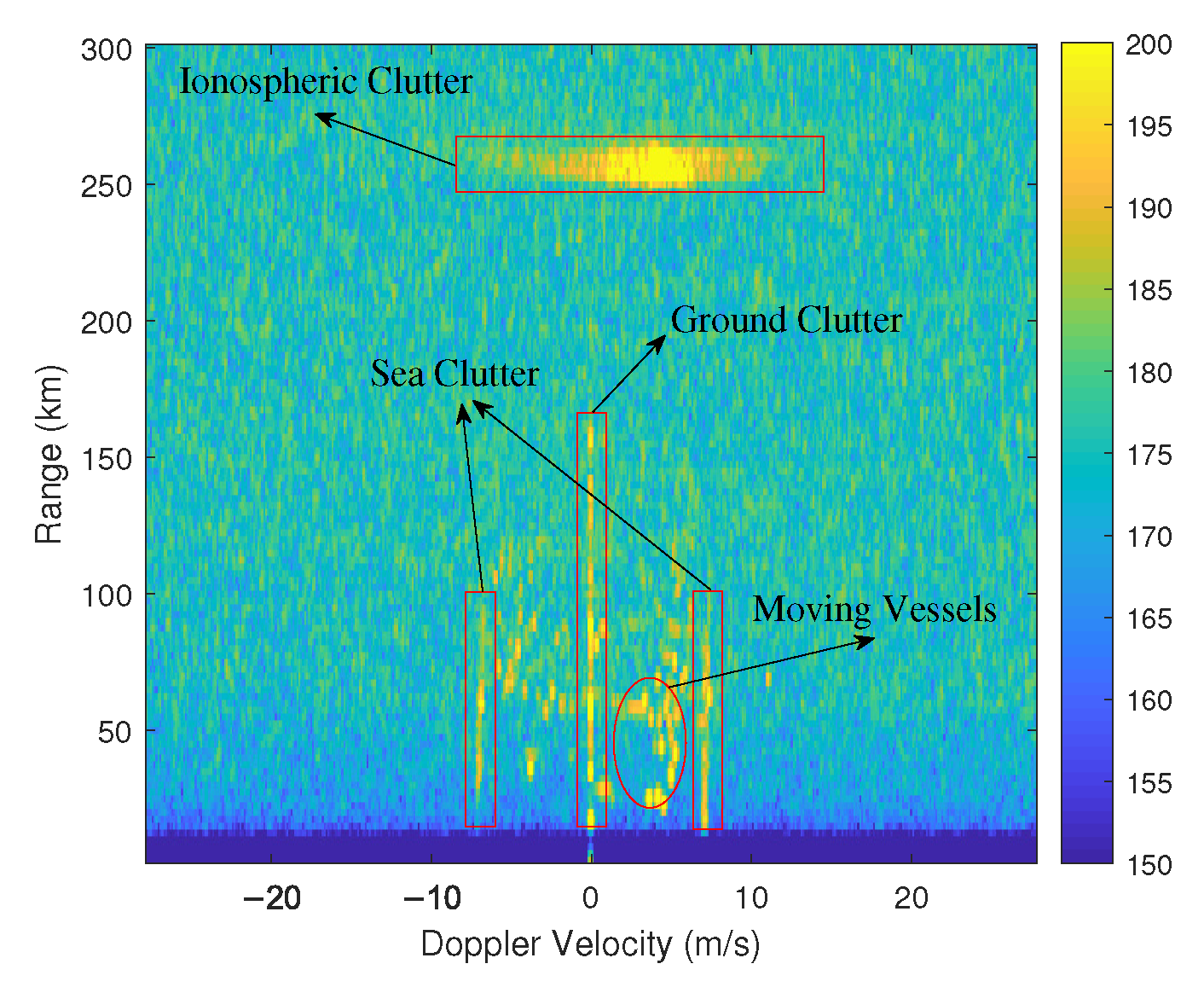
However, the backscattered echoes received by a compact HFSWR are a mixture of moving vessel echoes, background noise and various clutters such as sea clutter, ground clutter, ionospheric clutter, etc. [21,22,23,24], as shown in Figure 1. Some false alarms from clutters or noise are often mistakenly regarded as moving vessel plots, so the detected plot set of compact HFSWR usually contains a large number of false plots, which negatively affects moving vessel tracking algorithms.

2.2. Feature Analysis of Moving Vessels, Clutters, and Noise

It can be observed from Figure 1 that moving vessels and clutters have different features on an R-D map. The change of color depth indicates the transition of echo spectrum amplitudes. In this R-D map, moving vessels appear as isolated polygons with echo spectrum amplitudes decreased from centroids to peripheries. Ground and sea clutters spread within certain Doppler velocity bands along range dimension. Ionospheric clutter is strip-shaped along Doppler velocity dimension and widened to a certain extent along range dimension [25]. Background noise exists in the form of isolated points or local fluctuations on the R-D map. The difference in the features of moving vessels, various clutters, and noise in spatial correlation of echo spectrum amplitudes and position can be used for plot classification. Here, the spatial correlation characterizes the distribution of echo spectrum amplitudes of an area on an R-D map. The position means where a plot is obtained from an R-D map.

2.3. Moving Vessel Tracking

A moving vessel tracking algorithm, consisting of track initiation, track maintenance, and track termination, is applied to the obtained plot data sequence to produce moving vessel tracks. Track maintenance is an iterative process of state prediction, plot-to-track association, and state estimation, which are described as follows.

(1)

The motion and measurement models

The converted measurement Kalman filter (CMKF) [26] is used for state prediction and estimation in this paper, which is based on a motion model and a measurement model.

In general, vessels move at a constant velocity on the sea surface; the moving vessel motion model can be defined in a Cartesian coordinate system as

$${\mathbf{s}}_k=\mathbf{A}{\mathbf{s}}_{k-1}+{\mathit{\omega }}_{k-1},$$

(6)

where ${\mathbf{s}}_k={\left[x_k,v_{x_k},y_k,v_{y_k}\right]}^{\mathrm{T}}$ denotes the true moving vessel state vector at time k, $x_k$, $y_k$; and $v_{x_k}$, $v_{y_k}$ are the moving vessel’s position and velocity components along the x-axis and y-axis, respectively. ${\mathit{\omega }}_{k-1}$ denotes the process noise with zero mean and a covariance matrix ${\mathbf{G}}_{k-1}$. $\mathbf{A}$ is the state transition matrix defined as

$$\mathbf{A}=\left[\begin{array}{cccc}\hfill 1\hfill & \hfill T\hfill & \hfill 0\hfill & \hfill 0\hfill \\ \hfill 0\hfill & \hfill 1\hfill & \hfill 0\hfill & \hfill 0\hfill \\ \hfill 0\hfill & \hfill 0\hfill & \hfill 1\hfill & \hfill T\hfill \\ \hfill 0\hfill & \hfill 0\hfill & \hfill 0\hfill & \hfill 1\hfill \end{array}\right],$$

(7)

where T denotes the sampling time interval.

The measurement model is defined in the Cartesian coordinate as

$${\tilde{\mathbf{s}}}_k=\mathbf{M}{\mathbf{s}}_k+{\mathit{\eta }}_k,$$

(8)

where ${\tilde{\mathbf{s}}}_k={\left[{\tilde{x}}_k,{\tilde{v}}_{x_k},{\tilde{y}}_k,{\tilde{v}}_{y_k}\right]}^{\mathrm{T}}$ denotes the measured moving vessel state vector at time k, ${\tilde{x}}_k$, ${\tilde{y}}_k$; and ${\tilde{v}}_{x_k}$, ${\tilde{v}}_{y_k}$ are the measured position and velocity components along the x-axis and y-axis, respectively. ${\mathit{\eta }}_k$ represents the measurement noise with zero-mean and a covariance matrix ${\mathbf{R}}_k$. The measurement matrix $\mathbf{M}$ is an identity matrix defined as

$$\mathbf{M}=\left[\begin{array}{cccc}\hfill 1\hfill & \hfill 0\hfill & \hfill 0\hfill & \hfill 0\hfill \\ \hfill 0\hfill & \hfill 1\hfill & \hfill 0\hfill & \hfill 0\hfill \\ \hfill 0\hfill & \hfill 0\hfill & \hfill 1\hfill & \hfill 0\hfill \\ \hfill 0\hfill & \hfill 0\hfill & \hfill 0\hfill & \hfill 1\hfill \end{array}\right].$$

(9)

(2)

State prediction

Denote ${\mathbf{track}}_k=\{{\mathbf{P}}_1,{\mathbf{P}}_2,...,{\mathbf{P}}_N\}$ as a track being maintained with N plots at time k. The predicted state ${\widehat{\mathbf{s}}}_{k\mid k-1}={\left[{\widehat{x}}_{k\mid k-1},{\widehat{v}}_{x_{k\mid k-1}},{\widehat{y}}_{k\mid k-1},{\widehat{v}}_{y_{k\mid k-1}}\right]}^{\mathrm{T}}$ at time k can be calculated using the estimated state ${\widehat{\mathbf{s}}}_{k-1}={\left[{\widehat{x}}_{k-1},{\widehat{v}}_{x_{k-1}},{\widehat{y}}_{k-1},{\widehat{v}}_{y_{k-1}}\right]}^{\mathrm{T}}$ at time $k-1$ by

$${\widehat{\mathbf{s}}}_{k\mid k-1}=\mathbf{A}{\widehat{\mathbf{s}}}_{k-1}.$$

(10)

The corresponding state prediction error covariance matrix ${\widehat{\mathbf{E}}}_k$ is calculated as

$${\widehat{\mathbf{E}}}_k=\mathbf{A}{\mathbf{E}}_{k-1}{\mathbf{A}}^{\mathrm{T}}+{\mathbf{G}}_{k-1},$$

(11)

where ${\mathbf{E}}_{k-1}$ is the state estimation error covariance matrix at time $k-1$.

Since radar measures moving vessels in a polar coordinate system, the predicted state is converted from ${\widehat{\mathbf{s}}}_{k\mid k-1}$ in the Cartesian coordinate to ${\mathbf{P}}_k^{\mathrm{p}}={\left[v_k^{\mathrm{p}},r_k^{\mathrm{p}},{\theta }_k^{\mathrm{p}}\right]}^{\mathrm{T}}$ in the polar coordinate for subsequent plot-to-track association by

$$\begin{array}{c}{v}_k^{\mathrm{p}}=\frac{{\widehat{x}}_{k\mid k-1}{\widehat{v}}_{x_{k\mid k-1}}+{\widehat{y}}_{k\mid k-1}{\widehat{v}}_{y_{k\mid k-1}}}{\sqrt{{\widehat{x}}_{k\mid k-1}^2+{\widehat{y}}_{k\mid k-1}^2}},\\ r_k^{\mathrm{p}}=\sqrt{{\widehat{x}}_{k\mid k-1}^2+{\widehat{y}}_{k\mid k-1}^2},\\ {\theta }_k^{\mathrm{p}}=arctan\left(\frac{{\widehat{y}}_{k\mid k-1}}{{\widehat{x}}_{k\mid k-1}}\right).\end{array}$$

(12)

(3)

Plot-to-track association

In a preset association gate at time k, a measured plot ${\mathbf{P}}_k^{\mathrm{m}}={\left[v_k^{\mathrm{m}},r_k^{\mathrm{m}},{\theta }_k^{\mathrm{m}}\right]}^{\mathrm{T}}$ with the highest similarity to the predicted state ${\mathbf{P}}_k^{\mathrm{p}}={\left[v_k^{\mathrm{p}},r_k^{\mathrm{p}},{\theta }_k^{\mathrm{p}}\right]}^{\mathrm{T}}$ is selected to associate with the current track. The measured state vector ${\mathbf{P}}_k^{\mathrm{m}}={\left[v_k^{\mathrm{m}},r_k^{\mathrm{m}},{\theta }_k^{\mathrm{m}}\right]}^{\mathrm{T}}$ is then converted to the Cartesian coordinate to obtain the corresponding measured state ${\overline{\mathbf{s}}}_k={\left[{\overline{x}}_k,{\overline{v}}_{x_k},{\overline{y}}_k,{\overline{v}}_{y_k}\right]}^{\mathrm{T}}$ according to

$$\begin{array}{c}{\overline{x}}_k=r_k^{\mathrm{m}}cos{\theta }_k^{\mathrm{m}},\\ {\overline{y}}_k=r_k^{\mathrm{m}}sin{\theta }_k^{\mathrm{m}},\\ {\overline{v}}_{x_k}=\left({\overline{x}}_k-{\overline{x}}_{k-1}\right)/T,\\ {\overline{v}}_{y_k}=\left({\overline{y}}_k-{\overline{y}}_{k-1}\right)/T.\end{array}$$

(13)

(4)

State estimation

The estimated state ${\widehat{\mathbf{s}}}_k={\left[{\widehat{x}}_k,{\widehat{v}}_{x_k},{\widehat{y}}_k,{\widehat{v}}_{y_k}\right]}^{\mathrm{T}}$ at time k and the state estimation error covariance matrix ${\mathbf{E}}_k$ are updated by

$$\begin{array}{c}{\mathbf{K}}_k={\widehat{\mathbf{E}}}_k{\mathbf{M}}^{\mathrm{T}}{\left(\mathbf{M}{\widehat{\mathbf{E}}}_k{\mathbf{M}}^{\mathrm{T}}+{\mathbf{R}}_k\right)}^{-1},\\ {\widehat{\mathbf{s}}}_k={\widehat{\mathbf{s}}}_{k\mid k-1}+{\mathbf{K}}_k\left({\overline{\mathbf{s}}}_k-\mathbf{M}{\widehat{\mathbf{s}}}_{k\mid k-1}\right),\\ {\mathbf{E}}_k={\widehat{\mathbf{E}}}_k-{\mathbf{K}}_k\mathbf{M}{\widehat{\mathbf{E}}}_k,\end{array}$$

(14)

where ${\mathbf{K}}_k$ is the Kalman gain at time k. The estimated state ${\widehat{\mathbf{s}}}_k$ is used to update the current track.

The above procedure, including state prediction, plot-to-track association, and state estimation, is iteratively executed with subsequent new plot data to update the track continuously until it is terminated.

3. Methodology

In this section, the proposed plot quality evaluation and plot-to-track association methods are presented in detail. The plot quality evaluation method, including plot feature extraction module, feature normalization module, plot quality index calculation module, and plot quality level determination module, is introduced in Section 3.1. The obtained plot quality index is then employed as an auxiliary feature to produce the plot-to-track association method, which is described in Section 3.2.

3.1. Plot Quality Evaluation

Considering different features of moving vessels, clutters, and noise analyzed in Section 2.2, a plot quality evaluation method based on spatial correlation of echo spectrum amplitudes and position of plots is proposed to indicate the possibility of plots originating from moving vessels, clutters, and noise.

3.1.1. Plot Feature Extraction

In general, only kinematic parameters including range, azimuth, and Doppler velocity are used to characterize a plot measured by HFSWR. These kinematic parameters have limited capability in distinguishing plots of moving vessels, clutters, or noise [27]. It is noted that besides these kinematic parameters, their feature differences in plots from an R-D map can also be used to improve the moving vessel detection performance. Based on this consideration, the multi-directional gradient, local variance, and plot position probability obtained from an R-D map are combined to evaluate the plot quality. These features are respectively described as follows.

• Multi-directional gradient

Sea clutter, ground clutter, and ionospheric clutter usually occupy large and continuous areas on an R-D map, and their echo spectrum amplitudes vary gradually along the dimension of range or Doppler velocity [28]. In contrast, the plots from moving vessels usually appear like isolated points or clusters, and their gradients of echo spectrum amplitudes decrease gradually in eight directions around the peak points. The plots from noise also appear in the form of isolated points or clusters, but their echo spectrum amplitudes are relatively low without obvious gradient descent along all directions. Therefore, the multi-directional gradient variations can be used to distinguish different plots.

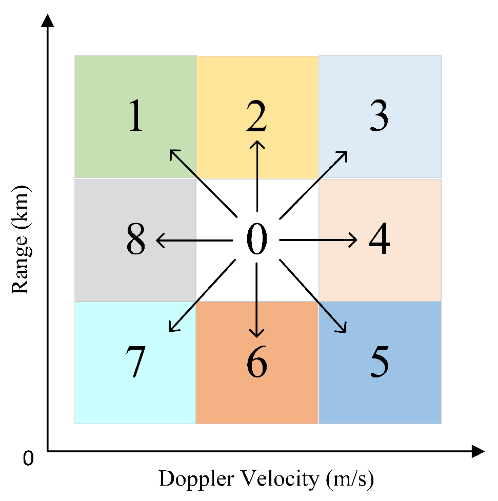
The schematic diagram for calculating multi-directional gradient is illustrated in Figure 2.

Figure 2 shows a $3\times 3$ cells configuration. Suppose the center cell (labeled as ’0’) is the one to be detected, if its echo spectrum amplitude exceeds the detection threshold derived from the CFAR algorithm and is determined as a peak point [29,30], one gradient value is calculated for each of its eight neighbor cells (labeled as ’1’–’8’) as

$${Grad}_i=\frac{A_0-A_i}{A_0}(i=1,2,...,8),$$

(15)

where ${Grad}_i$ denotes the gradient value for the ith direction, $A_0$ is the echo spectrum amplitude of the center cell, and $A_i$ is the echo spectrum amplitude of the neighbor cell in the ith direction. Since the center cell is determined as a peak point, its magnitude is higher than those of the other eight cells, the value of each ${Grad}_i$ is thus always positive.

It is noticed that the plots originated from clutters or noise may also have large gradient values along several directions. However, the gradient changes of the moving vessel plots generally have larger values in more directions. Thus, a gradient threshold U and a threshold V for the number of directions along which the gradient values exceed the threshold U are set to identify moving vessel plots according to the following rules: the number of ${Grad}_i$ that exceeds U is calculated as the feature value of multi-directional gradient and denoted as $X_{\mathrm{M}}$. The higher $X_{\mathrm{M}}$ is, the more likely the plot belongs to a moving vessel. If $X_{\mathrm{M}}$ is lower than V, the corresponding plot is regarded as a false plot.

• Local variance

The moving vessel plots located at the edge of clutters usually have smaller gradient values due to clutter, they cannot be easily identified based only on the multi-directional gradient feature. It is observed that ground clutter, sea clutter, and ionospheric clutter all have strong spatial correlation in echo spectrum amplitudes which are relatively high and evenly distributed in certain concentrated areas and have small local variances. The echo spectrum amplitudes of false plots from noise are low and also have small local variances. Different from clutters and noise, the moving vessel plots are isolated points on an R-D map, the echo spectrum amplitudes of them are relatively high and, thus, usually have weak spatial correlation and large local variance. As local variance reflects the variability of echo spectrum amplitudes in a certain area of a plot, it is employed as another feature for plot quality evaluation.

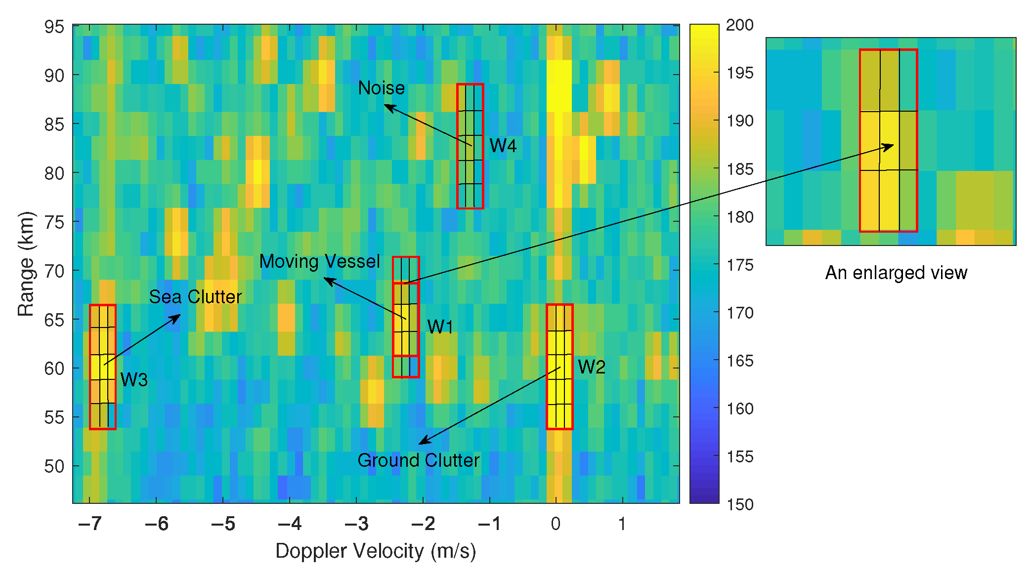
In order to calculate the local variance, a reference window surrounding a plot needs to be set. Figure 3 illustrates the variation characteristics of echo spectrum amplitudes of sea clutter, ground clutter, noise, and moving vessel plots on an R-D map. It can be seen that the echo spectrum amplitudes of sea clutter and ground clutter usually span three resolution cells along Doppler velocity dimension. As illustrated in the enlarged view, the echo spectrum amplitudes of a moving vessel span about nine resolution cells. The reference window should cover the area corresponding to the echo spectra of a moving vessel but should not be set too large to reduce the computational burden. With the aforementioned factors into consideration, a reference window with a size of $5\times 3$ is used to calculate the local variance in this article.

Four reference windows of moving vessel, ground clutter, sea clutter, and background noise, denoted as ${\mathrm{W}}_1$, ${\mathrm{W}}_2$, ${\mathrm{W}}_3$, and ${\mathrm{W}}_4$, are illustrated in Figure 3. It can be seen that the dispersion degree of echo spectrum amplitudes of the moving vessel is larger than that of clutter and background noise. Therefore, the local variance of echo spectrum amplitudes of a moving vessel is usually larger than that of false plots.

The local variance $X_{\mathrm{V}}$ is calculated as

$$X_{\mathrm{V}}=\frac{1}{n}\sum _{j=1}^n{\left(A_j-\mu \right)}^2,$$

(16)

where n represents the number of cells contained in the reference window, $A_j$ is the echo spectrum amplitude of the $j\mathrm{th}$ cell, and $\mu$ is the average echo spectrum amplitude of all the cells within the reference window.

• Plot position probability

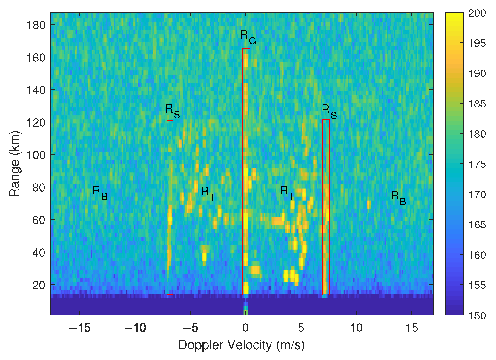
Since not all echo spectrum amplitudes of clutters are normally distributed, the multi-directional gradient and local variance of some false plots located in clutter regions are similar to those of moving vessel plots, they may be misclassified as moving vessels. It is noticed that an R-D map can be divided into different regions [31] according to different characteristics of clutters, noise, and moving vessels, as illustrated in Figure 4. ${\mathrm{R}}_{\mathrm{S}}$ is near the first-order peaks, ${\mathrm{R}}_{\mathrm{G}}$ is near zero Doppler frequency, ${\mathrm{R}}_{\mathrm{B}}$ contains the cells at far range with little echo. It is observed that both sea clutter and ground clutter extend 3–5 resolution cells along Doppler velocity dimension. Most moving vessels appear in the regions between sea clutter and ground clutter, and the rest of an R-D map is generally considered as background noise region. In Figure 4, ${\mathrm{R}}_{\mathrm{T}}$, ${\mathrm{R}}_{\mathrm{S}}$, ${\mathrm{R}}_{\mathrm{G}}$, and ${\mathrm{R}}_{\mathrm{B}}$ denote regions of moving vessels, sea clutter, ground clutter, and background noise, respectively. In these four regions, the probability that a real moving vessel may appear is ${Prob}_{{\mathrm{R}}_{\mathrm{T}}}>{Prob}_{{\mathrm{R}}_{\mathrm{S}}}>{Prob}_{{\mathrm{R}}_{\mathrm{G}}}>{Prob}_{{\mathrm{R}}_{\mathrm{B}}}$. Plots located in different regions should have different weights in evaluating plot quality. Thus, the plot position probability, which refers to the probability that a plot locates in a certain area, is used as another feature and denoted as $X_{\mathrm{P}}$. For example, if a plot is located in the moving vessel region ${\mathrm{R}}_{\mathrm{T}}$, $X_{\mathrm{P}}$ is equal to ${Prob}_{{\mathrm{R}}_{\mathrm{T}}}$.

It is worth pointing out that the ionospheric clutter is not considered in this research.

3.1.2. Feature Normalization

The value ranges of multi-directional gradient, local variance, and plot position probability are quite different. In order to comprehensively fuse these features together, the min-max normalization is employed to normalize each feature value to $[0,1]$, which can be expressed as

$$X_{\mathrm{nor}}=\frac{X-X_{\min }}{X_{\max }-X_{\min }},$$

(17)

where X represents the original value of a certain feature, including the multi-directional gradient, local variance, and plot position probability. $X_{\min }$ and $X_{\max }$ denote the minimum and maximum values of one feature for all plots in an R-D map, and $X_{\mathrm{nor}}$ is the normalized value of this feature.

3.1.3. Plot Quality Index Calculation

The normalized feature values of multi-directional gradient, local variance, and plot position probability are denoted as $S_{\mathrm{M}}$, $S_{\mathrm{V}}$, and $S_{\mathrm{P}}$, respectively. These three values are calculated for each measured plot ${\mathbf{P}}_k^{\mathrm{m}}$. Each plot in an R-D map is assigned a plot quality index calculated by its $(S_{\mathrm{M}},S_{\mathrm{V}},S_{\mathrm{P}})$. Due to their different contribution in plot quality evaluation, they are weighted and integrated to comprehensively assess the plot quality. Denote $a_{\mathrm{M}}$, $a_{\mathrm{V}}$, $a_{\mathrm{P}}$ as the corresponding weights of multi-directional gradient, local variance, and plot position probability, the final plot quality index Q is formulated as

$$Q=a_{\mathrm{M}}{S}_{\mathrm{M}}+a_{\mathrm{V}}{S}_{\mathrm{V}}+a_{\mathrm{P}}{S}_{\mathrm{P}},$$

(18)

where $a_{\mathrm{M}}+a_{\mathrm{V}}+a_{\mathrm{P}}=1.$ The larger the Q is, the more likely a plot originates from a real moving vessel.

3.1.4. Plot Quality Level Determination

The quality indexes of all plots from each R-D map are calculated. To visualize the evaluation results and distinguish plots with different quality indexes, each plot in an R-D map is classified into one of the four quality levels according to its plot quality index. In this article, the K-Means clustering algorithm [32,33] is applied to the obtained plot quality indexes to produce four plot quality levels, named as Level 1 (high quality)–Level 4 (low quality). Higher level means better quality.

The proposed plot quality evaluation method is applied to the detected plots on an R-D map, each plot gets a quality index. On the one hand, some plots with lower quality indexes can be discarded to reduce the computational burden of subsequent moving vessel tracking algorithms. On the other hand, the plot quality index can be used as auxiliary information to improve the accuracy of plot-to-track association.

3.2. Plot Quality Aided Plot-to-Track Association in Dense Clutter

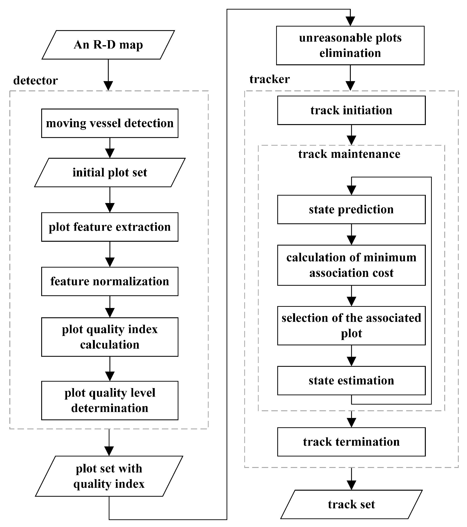
In order to improve the plot-to-track association accuracy, the plot quality index is combined with kinematic parameters to produce more comprehensive plot features, and a plot quality aided plot-to-track association method is proposed. It consists of three key steps, including unreasonable plots elimination, minimum association cost calculation, and associated plot selection. These key steps are described as follows.

3.2.1. Unreasonable Plots Elimination

In order to reduce the interference of false plots in plot-to-track association as well as the computational burden, the plots with unreasonable range and Doppler velocity can be filtered out before moving vessel tracking. Firstly, the effective detection range of compact HFSWR is usually between 15 km and 150 km due to its low transmit power and “range blind zone”; the plots with ranges outside this scope should be removed. Secondly, the vessel speed is generally less than 30 kn (15.43 m/s), the plots whose Doppler velocity exceeds 15.43 m/s are discarded. In addition, the plots with quality index less than a threshold $Q_{\min }$ are also eliminated.

3.2.2. Calculation of Minimum Association Cost

During the plot-to-track association procedure, an association gate is formed to include potential measured plots. For any measured plot ${\mathbf{P}}_{k+1}^{\mathrm{m}}={[v_{k+1}^{\mathrm{m}},r_{k+1}^{\mathrm{m}},{\theta }_{k+1}^{\mathrm{m}}]}^{\mathrm{T}}$ that falls into the association gate at time $k+1$, the association cost between it and ${\mathbf{track}}_k$ is calculated by

$$c=1-(c_v+c_r+c_{\theta }),$$

(19)

where $c_v$, $c_r$, and $c_{\theta }$ represent the similarity between ${\mathbf{P}}_{k+1}^{\mathrm{m}}$ and the predicted state ${\mathbf{P}}_{k+1}^{\mathrm{p}}$ of ${\mathbf{track}}_k$ in Doppler velocity, range, and azimuth, respectively, which are calculated by

$$\begin{array}{cc}\hfill & \hfill c_v=w_v\times \exp (-|v_{k+1}^{\mathrm{p}}-v_{k+1}^{\mathrm{m}}{|}^2/{\sigma }_v^2),\hfill \\ \hfill & \hfill c_r=w_r\times \exp (-|r_{k+1}^{\mathrm{p}}-r_{k+1}^{\mathrm{m}}{|}^2/{\sigma }_r^2),\hfill \\ \hfill & \hfill c_{\theta }=w_{\theta }\times \exp (-|{\theta }_{k+1}^{\mathrm{p}}-{\theta }_{k+1}^{\mathrm{m}}{|}^2/{\sigma }_{\theta }^2),\hfill \end{array}$$

(20)

where ${\sigma }_v$, ${\sigma }_r$, and ${\sigma }_{\theta }$ denote the standard deviations calculated using the data from all collected tracks within the coverage area of the radar, they are used to represent the average measurement errors of different kinematic parameters of the radar system. Once determined, they are applied for all tracks. It should be noted that the standard deviation ${\sigma }_{\theta }$ would be large for vessels detected at a distance. However, limited by the amount of field moving vessel data, ${\sigma }_{\theta }$ cannot be set adaptively according to the moving vessel range. When more moving vessel data are available, an adaptive setting method for these parameters should be investigated. $w_v$, $w_r$, and $w_{\theta }$ represent their corresponding association weights and satisfy

$$w_v+w_r+w_{\theta }=1,$$

(21)

where the values of $w_v$, $w_r$, and $w_{\theta }$ are set according to the radar measurement resolutions of Doppler velocity, range, and azimuth, respectively. It should be pointed out that the accurate Doppler velocity estimated by HFSWR is employed here to calculate the association cost.

The larger the values of $c_v$, $c_r$, and $c_{\theta }$ are, the smaller the association cost c is, and the higher the probability that the measured plot belongs to ${\mathbf{track}}_k$ is. Assume there are M measured plots in the association gate at time $k+1$, an association cost set $\left\{c_1,c_2,...,c_M\right\}$ between each measured plot and the current track can be calculated by Equation (5), and then the minimum association cost $c_{\min }=\min \left\{c_1,c_2,...,c_M\right\}$ can be obtained.

3.2.3. Selection of the Associated Plot

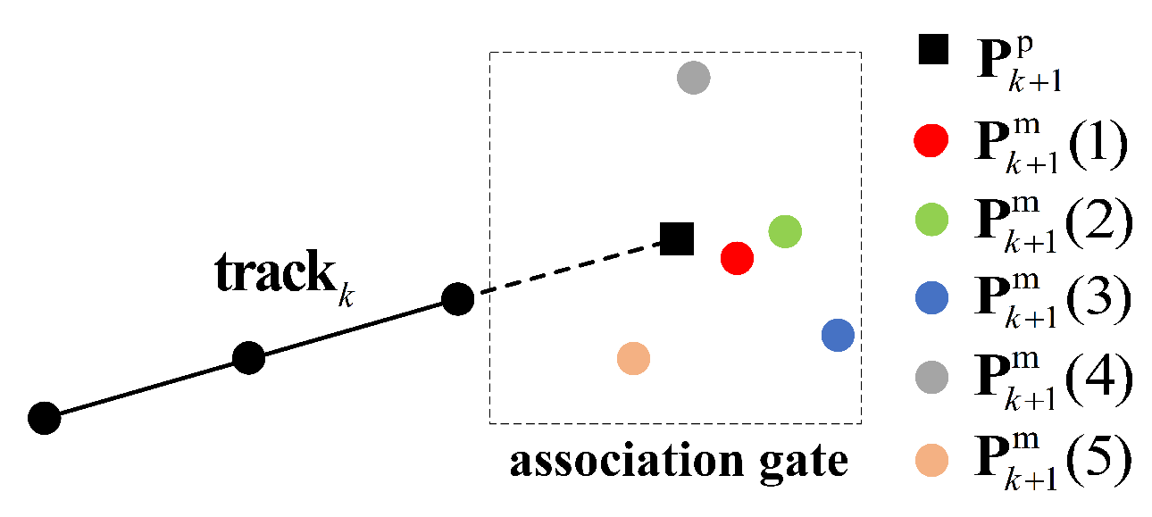
As the kinematic parameters of false plots may be similar to those of moving vessel plots, the plot nearest to the predicted moving vessel state is not necessarily derived from a real moving vessel. An illustrative example is shown in Figure 5. The predicted moving vessel state of ${\mathbf{track}}_k$ obtained at time k is ${\mathbf{P}}_{k+1}^{\mathrm{p}}$, the association gate centered at ${\mathbf{P}}_{k+1}^{\mathrm{p}}$ includes five measured plots $\{{\mathbf{P}}_{k+1}^{\mathrm{m}}\left(1\right),{\mathbf{P}}_{k+1}^{\mathrm{m}}\left(2\right),...,{\mathbf{P}}_{k+1}^{\mathrm{m}}\left(5\right)\}$ at time $k+1$. Suppose ${\mathbf{P}}_{k+1}^{\mathrm{m}}\left(1\right)$, ${\mathbf{P}}_{k+1}^{\mathrm{m}}\left(3\right)$, ${\mathbf{P}}_{k+1}^{\mathrm{m}}\left(4\right)$, and ${\mathbf{P}}_{k+1}^{\mathrm{m}}\left(5\right)$ are plots from clutters, and the plot quality indexes of them are denoted as $Q_1$, $Q_3$, $Q_4$, and $Q_5$, respectively, and they will be small. ${\mathbf{P}}_{k+1}^{\mathrm{m}}\left(2\right)$ is the measured plot of ${\mathbf{track}}_k$ at time $k+1$, its plot quality index is $Q_2$ and will be large. If the NNDA algorithm that only uses kinematic parameters is applied for plot-to-track association, the association cost of ${\mathbf{P}}_{k+1}^{\mathrm{m}}\left(1\right)$ takes the minimum value; thus, it will be associated with ${\mathbf{track}}_k$, leading to incorrect association. It can be seen that the association cost of ${\mathbf{P}}_{k+1}^{\mathrm{m}}\left(2\right)$ to ${\mathbf{track}}_k$ is comparable to that of ${\mathbf{P}}_{k+1}^{\mathrm{m}}\left(1\right)$, but $Q_2$ is much larger than $Q_1$; if the plot quality index is introduced into plot-to-track association, ${\mathbf{P}}_{k+1}^{\mathrm{m}}\left(2\right)$ will be selected for association.

Thus, in order to reduce the plot-to-track association errors caused by the interference of false plots, the plot quality index is employed as an auxiliary feature to increase the probability of selecting the true moving vessel plot in plot-to-track association. The plot quality index is incorporated into the minimum association cost-based NNDA method to determine the most likely associated plot. The proposed plot-to-track association method for a certain track ${\mathbf{track}}_k$ can be described as follows.

Step 1: The association costs $\left\{c_1,c_2,...,c_M\right\}$ between all M candidate plots $\{{\mathbf{P}}_{k+1}^{\mathrm{m}}\left(1\right),$${\mathbf{P}}_{k+1}^{\mathrm{m}}\left(2\right),...,{\mathbf{P}}_{k+1}^{\mathrm{m}}\left(M\right)\}$ in the association gate at time $k+1$ and the predicted moving vessel state ${\mathbf{P}}_{k+1}^{\mathrm{p}}$ are calculated, and the minimum association cost $c_{\min }=\min \left\{c_1,c_2,...,c_M\right\}$ is obtained.

Step 2: The difference between the association cost $c_i$ of the $i\mathrm{th}$ candidate plot and the minimum association cost $c_{\min }$ is denoted as $Dif{f}_i$ and calculated by

$${Diff}_i=c_i-c_{\min }(i=1,2,...,M).$$

(22)

Step 3: A threshold $\epsilon$ is set, if $Dif{f}_i\le \epsilon$, the $i\mathrm{th}$ candidate plot is determined as a preliminarily associated plot, then a preliminarily associated plot set $\{{\overline{\mathbf{P}}}_{k+1}^{\mathrm{m}}\left(1\right),{\overline{\mathbf{P}}}_{k+1}^{\mathrm{m}}\left(2\right),...,$${\overline{\mathbf{P}}}_{k+1}^{\mathrm{m}}\left(f\right)\}(1\le f\le M)$ is obtained.

Step 4: The plot with the highest quality index in the preliminarily associated plot set is selected as the associated plot.

Step 5: The selected associated plot is fused with the predicted moving vessel state ${\mathbf{P}}_{k+1}^{\mathrm{p}}$ to obtain the estimated moving vessel state at time $k+1$, then the current track is updated.

The flowchart of the proposed plot-to-track association method is shown in Figure 6.

4. Results of Experiments

To verify the performance of the proposed plot-to-track association method, moving vessel tracking experiments were carried out with field data of compact HFSWR using both the NNDA method and the proposed method, respectively. The automatic identification system (AIS) data were used as ground truth for the tracking results, the tracking time on moving vessels, which means the duration a moving vessel has been successfully tracked without fragmentation, was used as the evaluation index.

The experimental data were collected by a newly developed compact over-the-horizon radar for maritime surveillance (CORMS) system located at the shore of Bohai Bay in China. The system parameters of CORMS are listed in

Table 1. The system parameters of CORMS.

Specification	Value
Transmitting waveform	FMICW
Receiving antenna number	8
Working frequency (MHz)	4.7
Coherent integration time (s)	262.144
Data rate (frame/min)	1

. A total of 266 frames of data were collected from 11:04 a.m. to 3:29 p.m. on January 18, 2019.

Four thresholds U, V, $\epsilon$, and $Q_{\min }$ can be statistically calculated using field measurements. A track association method is applied to both radar and AIS tracks to find the associated track pairs. Then the plots measured by radar with matched AIS correspondences are identified as from real moving vessels. The data from these plot pairs are used to determine the thresholds.

(1)

Determination of U and V.

The gradients along eight directions of each selected moving vessel plot are calculated using Equation (15), and the mean value of the gradients from all moving vessel plots is used to set U. Then the number of directions in which the corresponding gradient exceeds U, denoted as $X_{\mathrm{M}}$, for each real moving vessel plot is calculated. The mean value of $X_{\mathrm{M}}\mathrm{s}$ obtained from all the moving vessel plots is set as the threshold V.

(2)

Determination of $\epsilon$.

For each identified real moving vessel track, the minimum association costs during plot-to-track association at each time instant are calculated using Equation (19). Then a dataset containing the minimum association costs from all real moving vessel tracks can be obtained. The standard deviation of this dataset is calculated and used to set $\epsilon$.

(3)

Determination of $Q_{\min }$.

The radar plots that can not be associated with any moving vessel track are identified as false plots. The plot quality index Q of real moving vessel plots and false plots are calculated using Equation (18). Then the histograms of Q for moving vessel and false plots are respectively obtained and fitted using probability density fitting. The abscissa value corresponding to the intersection of two fitting curves is determined as $Q_{\min }$.

(4)

Determination of $(a_{\mathrm{M}},a_{\mathrm{V}},a_{\mathrm{P}})$ and $(w_v,w_r,w_{\theta })$.

The two groups of weights $(a_{\mathrm{M}},a_{\mathrm{V}},a_{\mathrm{P}})$ and $(w_v,w_r,w_{\theta })$ are determined using the orthogonal experiment method [34] with different weight combinations under the constraint that the summation of all weights should be equal to one.

It should be pointed out that the above thresholds and weights only need to be set once for a radar system and can be used for all plots detected by this radar. Whether the corresponding parameters are applicable for other radar systems or not needs to be further investigated.

The parameters involved in the proposed method are listed in

Table 2. The parameters set for the proposed method in the experiment.

Parameter	Value
U	0.025
V	4
$\epsilon$	0.2
$Q_{\min }$	0.15
$\left(a_{\mathrm{M}},a_{\mathrm{V}},a_{\mathrm{P}}\right)$	(0.2, 0.4, 0.4)
$\left(w_v,w_r,w_{\theta }\right)$	(0.7, 0.2, 0.1)

.

4.1. Plot Quality Evaluation and Results Analysis

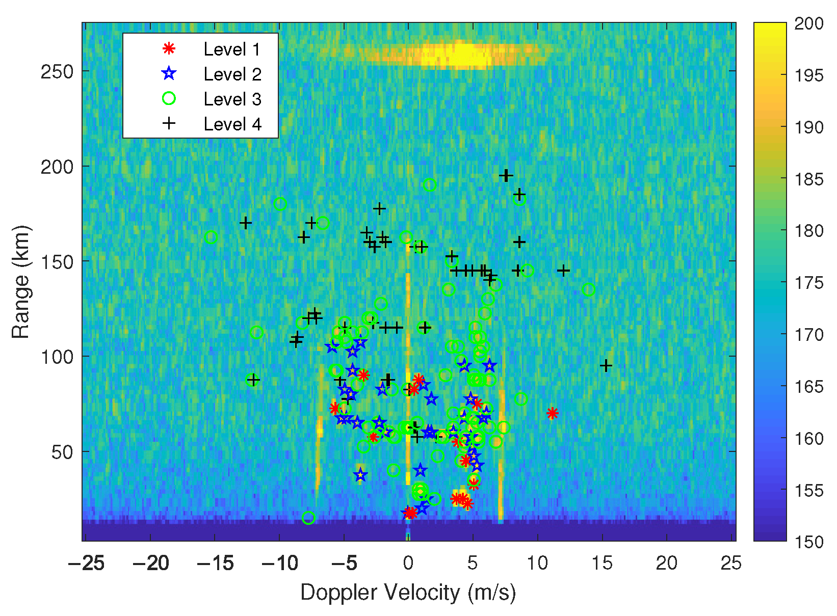
The effectiveness of the proposed plot quality evaluation method is evaluated first. Figure 7 shows the plot quality evaluation results for an R-D map obtained at 1:59 p.m.; the detected plots are divided into four levels according to their plot quality indexes. It can be visually seen that the plots in Level 1 have strong scattering intensity with high SNR, while the plots in Level 2 have lower scattering intensity. The plots in Level 3 look like weak moving vessels and some of them are located at the edge of clutters. The plots in Level 4 seem to be noise or clutter plots.

Next, the CMKF and the proposed plot-to-track association methods were applied to the plot data sequence collected from 11:04 a.m. to 3:29 p.m. to produce moving vessel tracks. The obtained tracks are associated with corresponding AIS tracks using the method proposed in [35].

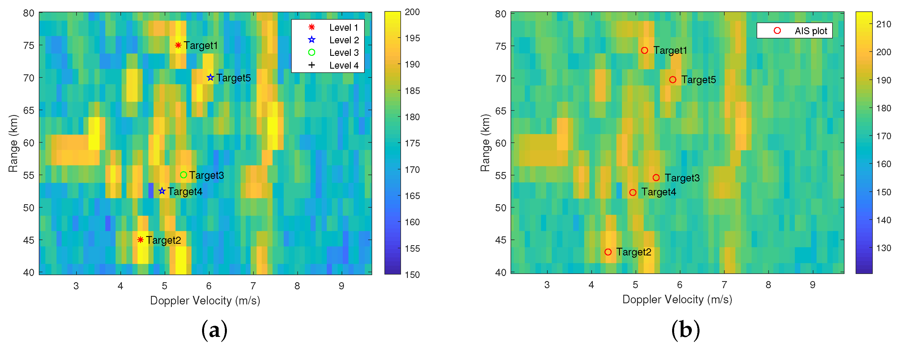
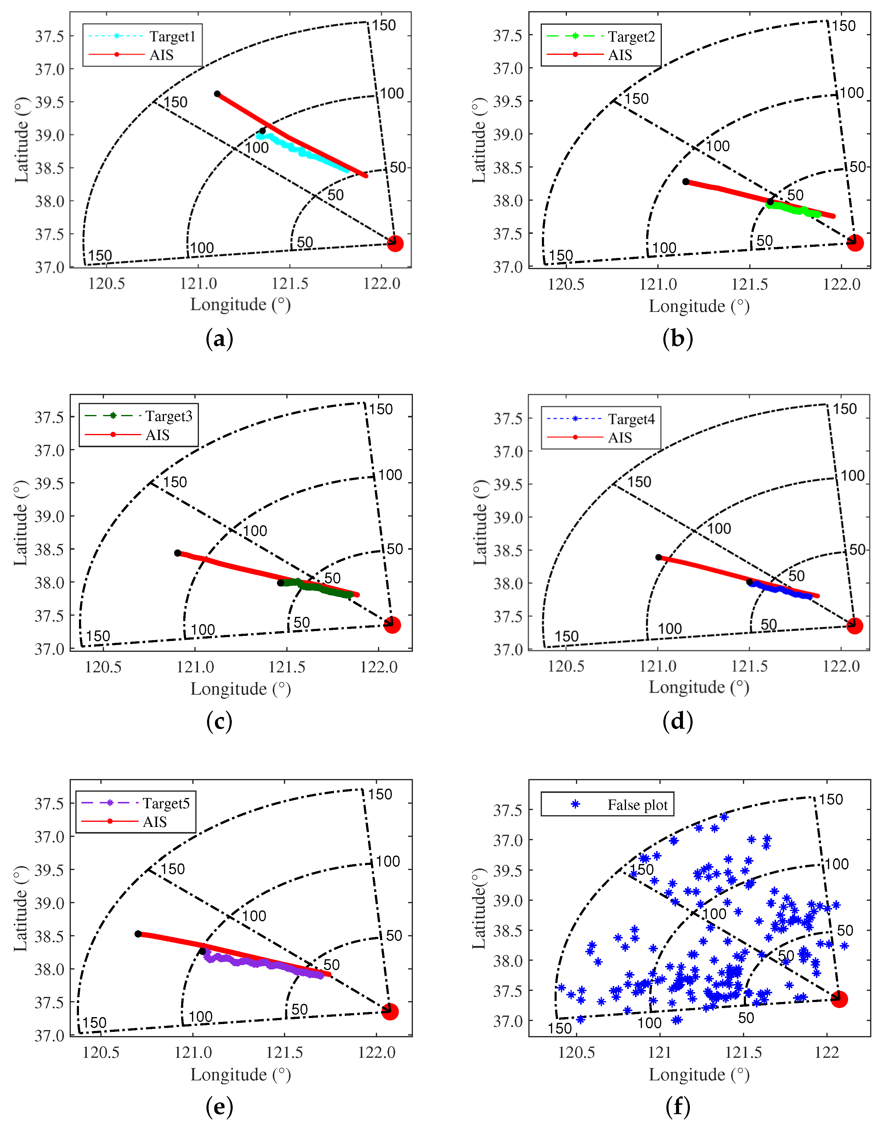
In order to quantitatively analyze the plot quality evaluation results, five moving vessels with matching AIS data are selected for further analysis. Figure 8 displays the plots of targets 1–5 and the corresponding AIS plots on an R-D map obtained at 1:59 p.m. Figure 9a–e depicts the tracks of targets 1–5 and their AIS tracks in geographic coordinate system, it is confirmed that they are derived from real moving vessels. The solid red dots indicate the radar location.

Twenty consecutive R-D maps during the common period of the five tracks, i.e., 1:59 p.m.–2:18 p.m. were selected, and ten false plots without being associated with any track in each R-D map were chosen for analysis. Figure 9f illustrates all the selected false plots in geographic coordinate system.

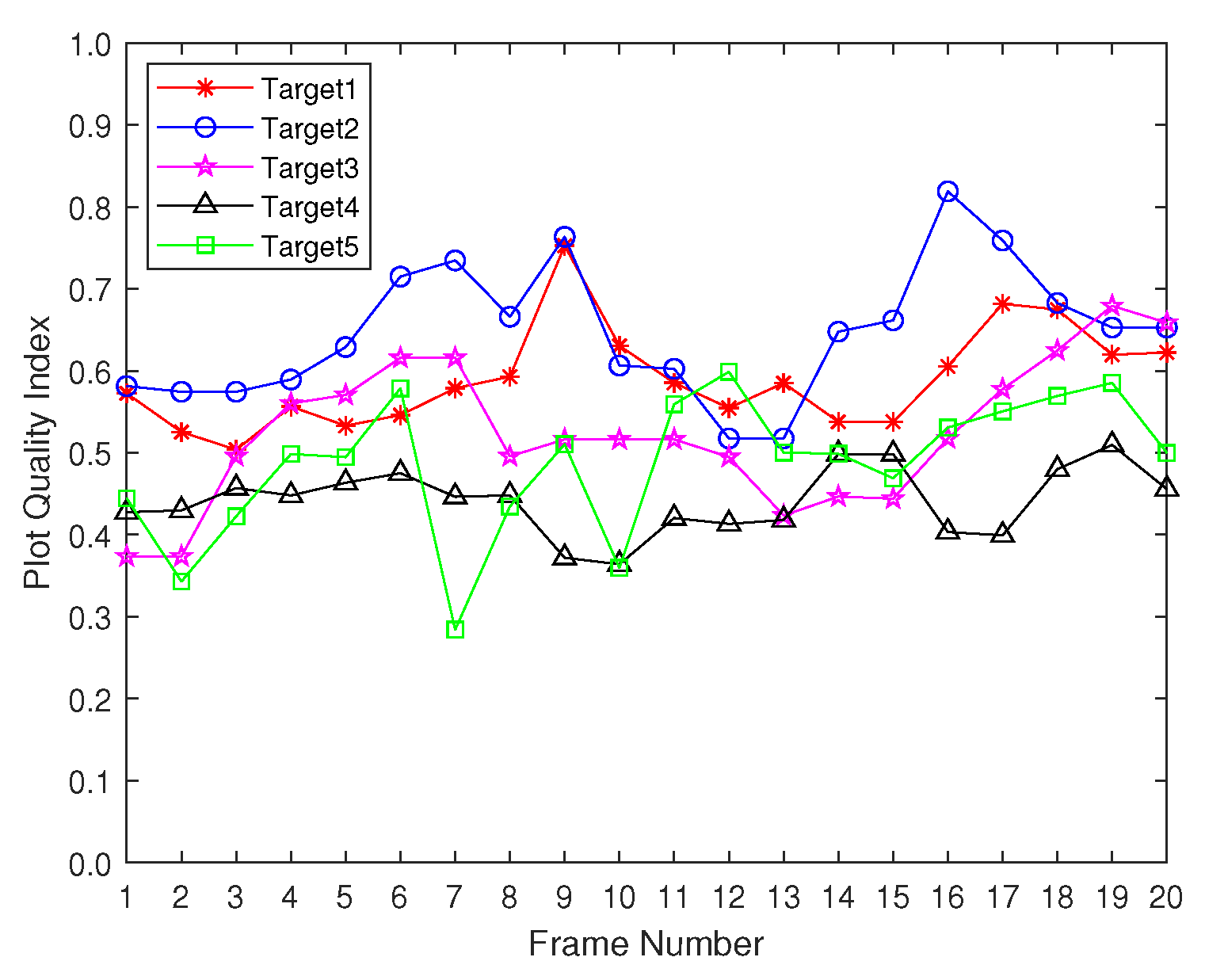
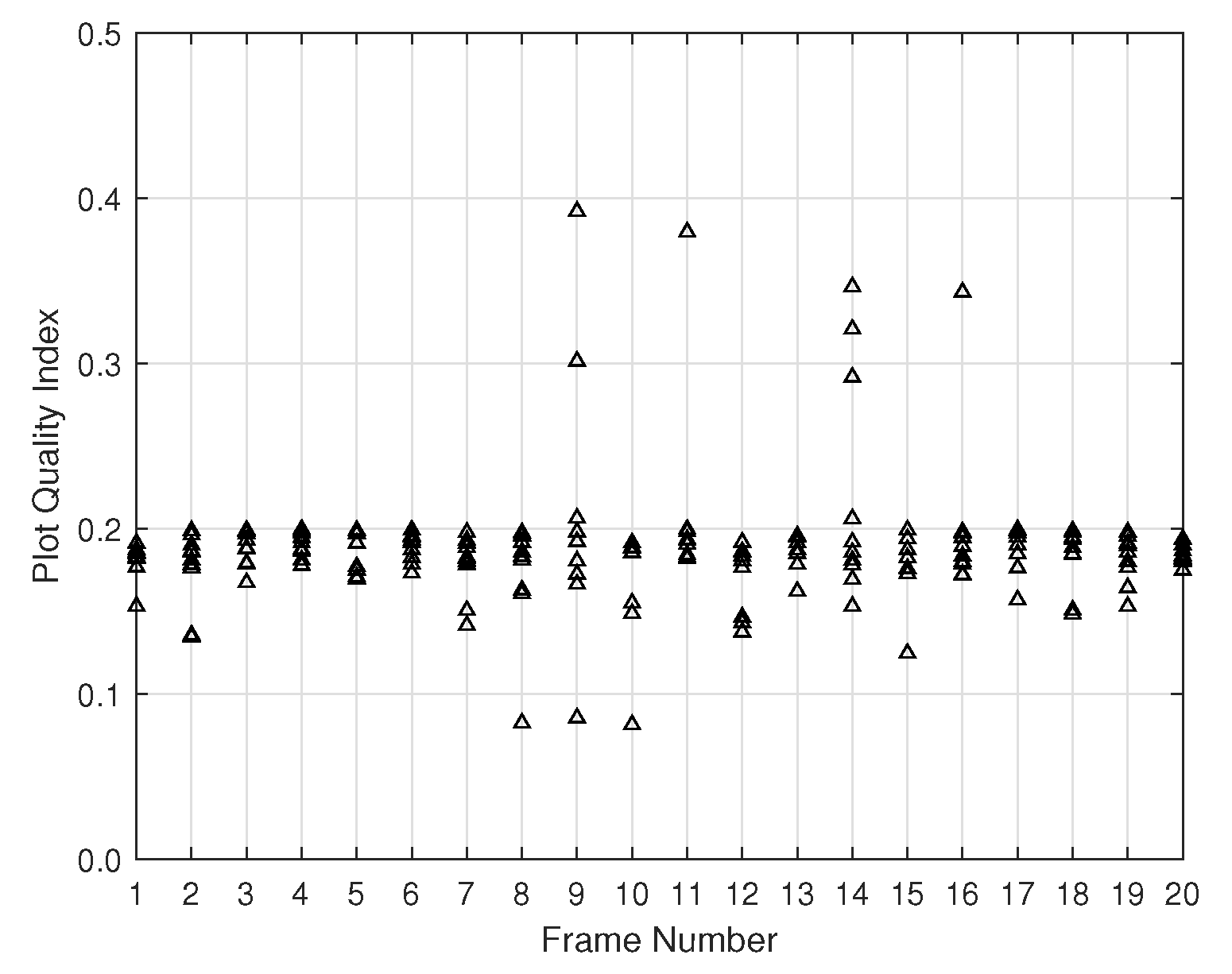
The plot quality indexes for both moving vessel and false plots were calculated and compared, the results are illustrated in Figure 10, Figure 11 and Figure 12.

The variation trends of plot quality index for five moving vessels are shown in Figure 10. It can be seen that the quality indexes of moving vessel plots are generally greater than 0.4. Only a few of them are less than 0.3 due to their weak echoes caused by RCS fluctuations. It should be noticed that the plot quality indexes of different moving vessels are similar; thus, they cannot be used to distinguish different moving vessels.

The plot quality indexes of all selected false plots are shown in Figure 11. It can be observed that the quality indexes of most false plots are around 0.2, only a few of them are greater than 0.3.

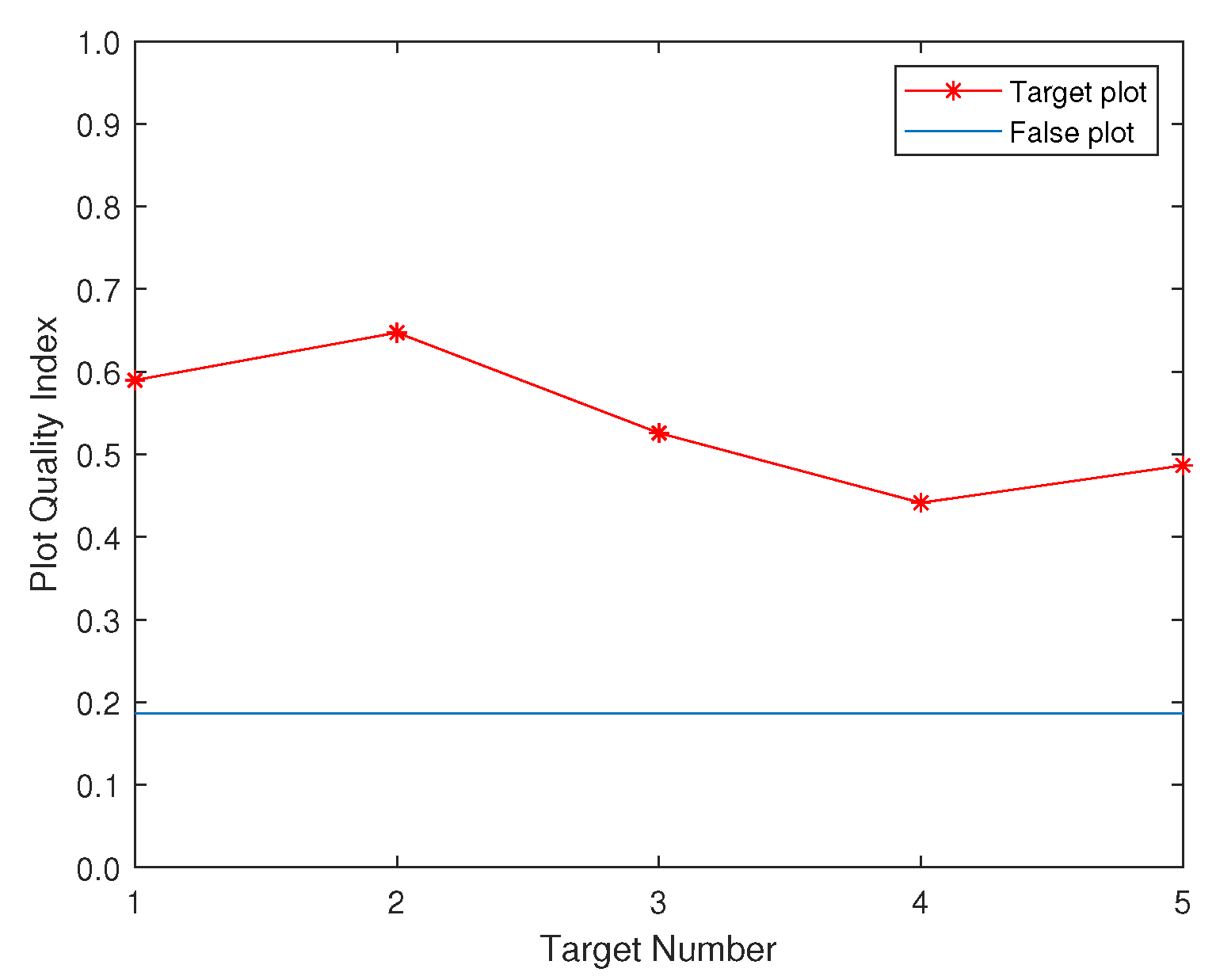
The average plot quality indexes of these five moving vessels and all false plots are shown in Figure 12, where the red asterisks are the average plot quality indexes for each moving vessel in twenty consecutive frames, and the blue horizontal line represents the average plot quality index of all false plots. As can be seen, the average plot quality indexes of the five moving vessels are much larger than that of the false plots.

It can be concluded from above experimental results that the plot quality indexes of moving vessel plots are higher than those of false plots. Therefore, the plot quality index can be used to distinguish moving vessel and false plots.

4.2. Analysis of Tracking Performance

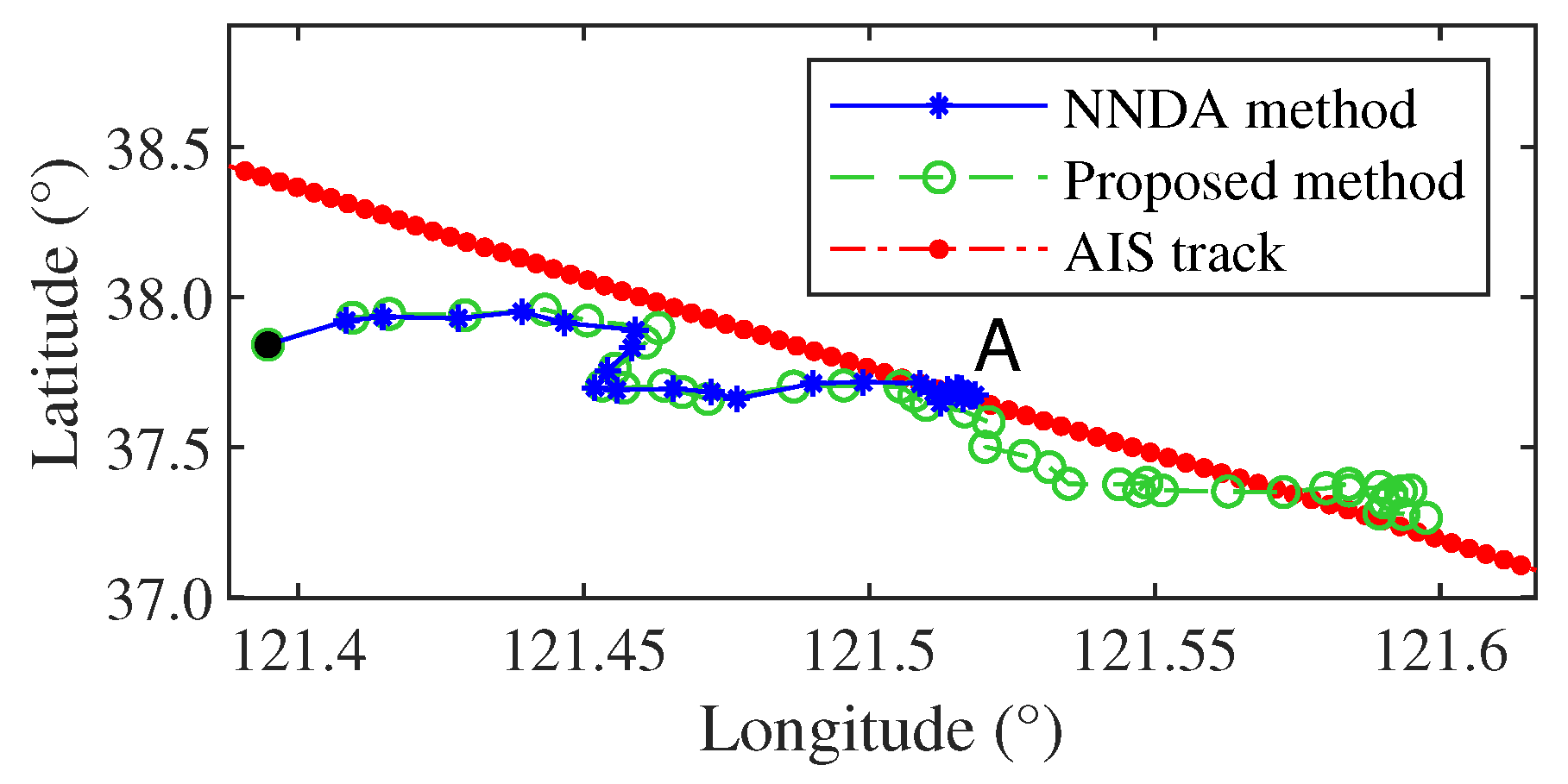
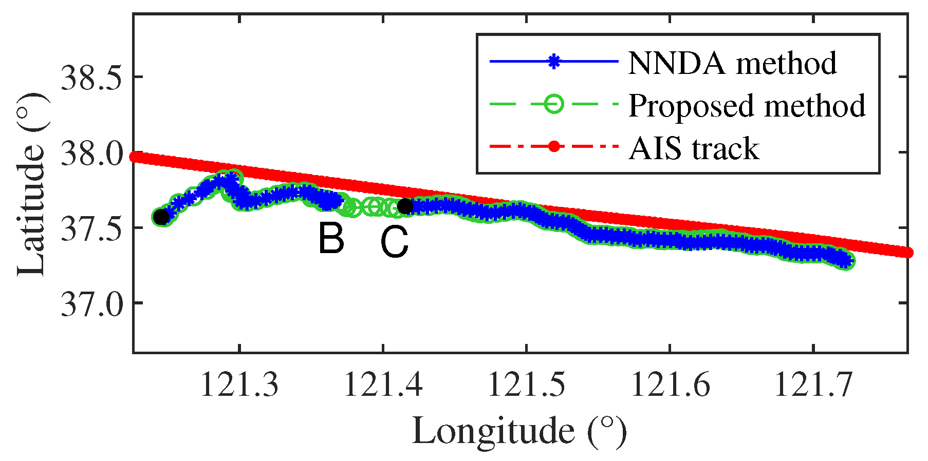
The NNDA and proposed plot-to-track association methods were respectively combined with the CMKF tracking method and applied for moving vessel tracking. Two fragmented tracks obtained by the NNDA method, labeled as T1 and T2, were selected for analysis. Both of them are heading towards the radar and have matching AIS data. The comparisons of tracking results are shown in Figure 13 and Figure 14. The blue and green tracks denote the tracking results obtained by the NNDA and proposed plot-to-track association methods, respectively. The red tracks are corresponding AIS tracks. The black solid circles represent the plots at the starting points.

(1)

Tracking results analysis of T1

As can be seen from Figure 13, the moving vessel track obtained by the NNDA method breaks at point A (1:07 p.m.). It was found that the Doppler velocity of this moving vessel at 1:04 p.m. is 8.04 m/s, which coincides with the Doppler velocities corresponding to first-order sea clutter. The track is associated with a false plot generated by sea clutter at 1:04 p.m., causing track fragmentation. The moving vessel track obtained by the proposed plot-to-track association method can be associated with a moving vessel plot at 1:04 p.m. and updated correctly. The tracking time on moving vessels increases by 17 min. Analysis of candidate plots in the association gate at 1:04 p.m. shows that the association cost of a clutter plot selected by the NNDA method and a moving vessel plot selected by the proposed method are 0.21 and 0.38, and the corresponding quality indexes are 0.18 and 0.40, respectively, i.e., their association costs are similar, but the quality index of the moving vessel plot is higher. It verifies that in dense clutter scenarios, the proposed plot-to-track association method can effectively distinguish moving vessel and clutter plots and improve the plot-to-track association accuracy.

(2)

Tracking results analysis of T2

It can be observed from Figure 14, the moving vessel track obtained by the NNDA method breaks at point B (1:59 p.m.) and restarts at point C (2:02 p.m.). The reason for track fragmentation is that the track is disturbed by a false plot at 1:56 p.m., and there are no consequent measured plots associated with it. As a result, the track is updated by predicted states in several consecutive frames and then is terminated. However, the moving vessel track obtained by the proposed plot-to-track association method is correctly associated with the moving vessel plot at 1:56 p.m. and the track is updated subsequently.

The quality indexes of the associated plots selected by the NNDA and proposed methods are 0.17 and 0.56, and the association cost of them are 0.21 and 0.25, respectively. Their association costs are similar, but the quality index of the moving vessel plot selected by the proposed method is much higher. It can be concluded that the the associated plot selected by the NNDA method may be a noise plot that leads to the plot-to-track association error. On the contrary, the proposed plot-to-track association method can join the two track segments obtained by the NNDA method successfully.

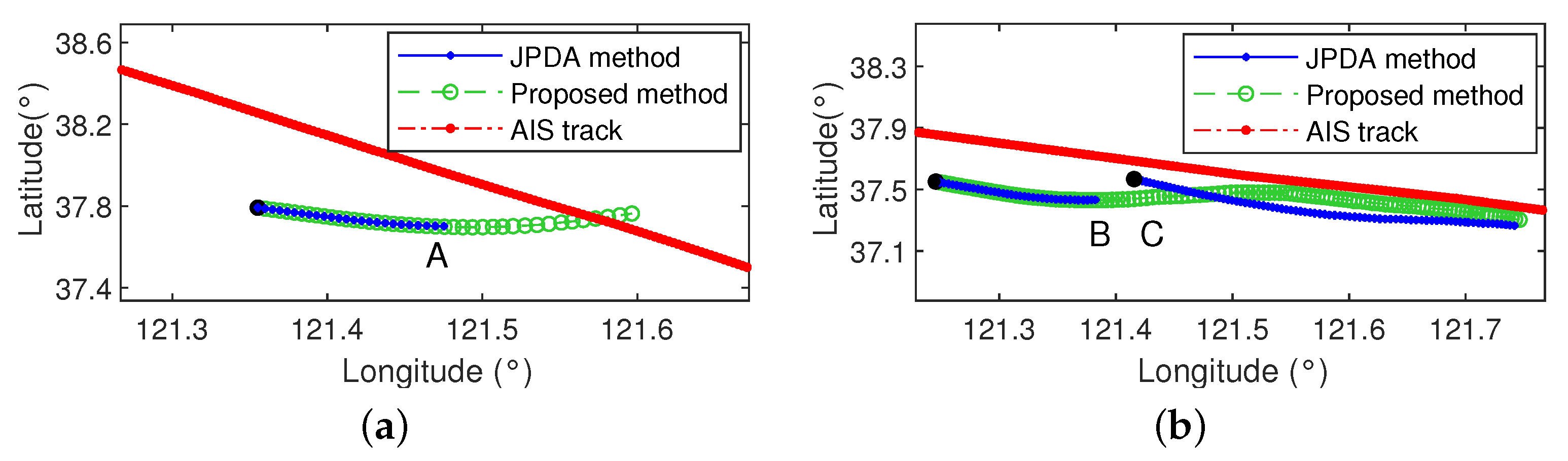
It is worth pointing out that the proposed plot quality index can also be combined with other plot-to-track association methods to improve their association accuracy. Since the JPDA method achieves good performance in multi-target tracking scenarios, the proposed plot quality index is introduced into the JPDA method to calculate the association probability of candidate plots within the association gate.

Plot-to-track association tests based on the JPDA method with and without plot quality index were also conducted on the two fragmented tracks T1 and T2, and the obtained tracking results are shown in Figure 15.

It can be seen that the tracks obtained by the JPDA method are smoother than those obtained by the NNDA method. However, due to the low positioning accuracy of compact HFSWR and the interference of clutter and noise, track fragmentations also occur when the original JPDA method is applied. Similar to the tracking results obtained by the NNDA method, the track T1 breaks at point A, and track T2 breaks at point B when the JPDA method is employed. After introducing the plot quality index, the fragmented tracks are extended or connected to produce longer tracks.

Considering that the JPDA method has high computational complexity and requires prior information on moving vessel quantity, it is not selected as the preferred method here.

4.3. Analysis of Computational Complexity

To analyze the computational complexity of the proposed method, two hundred Monte Carlo experiments were performed for the plot-to-track association procedure. The results show that the average running time of the proposed method is only increased by 0.21s compared with that of the NNDA method, which is much less than the radar data rate of 1 frame/min and meets the engineering requirements for real-time moving vessel tracking.

In addition, the plot quality index can be used to filter out some false plots as described in Section 3.2.1. Statistical analysis shows that about $32.6\%$ plots with lower quality indexes in each R-D map were filtered out, which effectively reduces the data processing burden of tracking algorithms.

4.4. Analysis of Parameter Sensitivity

Both plot quality evaluation and plot-to-track association performance depend on the settings of the four thresholds U, V, $\epsilon$, $Q_{\min }$ and two groups of weights $(a_{\mathrm{M}},a_{\mathrm{V}},a_{\mathrm{P}})$, $(w_v,w_r,w_{\theta })$. Once these parameters are determined, small deviations from the determined parameter values will have little influence on plot quality evaluation and plot-to-track association performance.

5. Discussion

From the above analysis, it can be summarized that:

(i)

The working environment of compact HFSWR is extremely complex and a great number of false plots may be produced, which will cause plot-to-track association errors for moving vessel tracking. The proposed plot quality evaluation method can effectively evaluate the quality of plots according to their quality indexes, which can be used to filter out some false plots and provide assistant information for resolving the plot-to-track association ambiguity.

(ii)

The plot quality evaluation method based on spatial correlation of echo spectrum amplitudes and plot position probability may not accurately classify moving vessel plots and false plots. However, the proposed plot quality index can indicate the possibility that a plot derives from a real moving vessel. The higher the plot quality index is, the more likely the plot comes from a real moving vessel.

(iii)

Experimental results show that the proposed plot quality evaluation method can reasonably calculate the quality indexes of most plots. However, it is worth noting that the extracted features of false plots may be similar to those of moving vessel plots since some clutter appears in the form of blocks, so the evaluation results of these plots may be inaccurate.

(iv)

The NNDA method only uses kinematic parameters to calculate the similarities between measured plots and moving vessel tracks. In dense clutter scenarios, it often causes false tracking and track fragmentation due to plot-to-track association errors. The proposed plot-to-track association method introduces the plot quality index as auxiliary information to collaboratively determine the associated plot. Experimental results show that this method can effectively increase tracking time on moving vessels and improve tracking continuity.

(v)

During the moving vessel tracking experiments, the authors found that the proposed plot-to-track association method has better tracking performance in dense clutter scenarios, but false tracking caused by the interference of adjacent moving vessels may occur in multi-target tracking scenarios. Because the plot quality indexes of different moving vessel plots may be similar, as shown in Figure 10, it is difficult to accurately distinguish the source of moving vessel plots by their quality indexes and kinematic parameters when multiple moving vessels are close to each other. Therefore, the optimal assignment of plot-track pairs in multi-target tracking scenarios needs to be further investigated.

6. Conclusions

To improve the plot-to-track association accuracy and enhance the moving vessel tracking performance of compact HFSWR, a plot quality aided plot-to-track association method for dense clutter scenarios is developed. The main contributions of this article are in two folds. Firstly, according to the spatial correlation of echo spectrum amplitudes and position of different plots on an R-D map, a plot quality evaluation method is proposed. The plot quality index calculated by this method can be applied to roughly distinguish moving vessel plots and false plots originating from clutters or noise, and some false plots can be filtered out. Secondly, the plot quality index can be used as auxiliary information to improve the plot-to-track association accuracy. Experimental results show that the proposed method reduces the data processing burden of tracking algorithms, improves the accuracy of plot-to-track association, and increases the continuity of moving vessel tracking in dense clutter scenarios. Thus, it can be applied to compact HFSWR systems to enhance tracking performance.

References

- Ji, Y.; Zhang, J.; Wang, Y.; Sun, W.; Li, M. Target Monitoring Using Small-aperture Compact High-frequency Surface Wave Radar. IEEE Aerosp. Electron. Syst. Mag. 2018, 33, 22–31. [Google Scholar] [CrossRef]
- Sun, W.; Pang, Z.; Huang, W.; Ma, P.; Ji, Y.; Dai, Y.; Li, X. A Multi-Stage Vessel Tracklet Association Method for Compact High-Frequency Surface Wave Radar. Remote Sens. 2022, 14, 1601. [Google Scholar] [CrossRef]
- Huang, W.; Gill, E.W. (Eds.) Ocean Remote Sensing Technologies—High-Frequency, Marine and GNSS-Based Radar; SciTech Publishing: Luxembourg, 2021. [Google Scholar]
- Sun, W.; Ji, M.; Huang, W.; Ji, Y.; Dai, Y. Vessel Tracking Using Bistatic Compact HFSWR. Remote Sens. 2020, 12, 1266. [Google Scholar] [CrossRef] [Green Version]
- Sun, W.; Huang, W.; Ji, Y.; Dai, Y.; Ren, P.; Zhou, P.; Hao, X. A Vessel Azimuth and Course Joint Re-Estimation Method for Compact HFSWR. IEEE Trans. Geosci. Remote Sens. 2020, 58, 1041–1051. [Google Scholar] [CrossRef]
- Sun, W.; Pang, Z.; Huang, W.; Ji, Y.; Dai, Y. Vessel Velocity Estimation and Tracking from Doppler Echoes of T/R-R Composite Compact HFSWR. IEEE J. Sel. Top. Appl. Earth Obs. Remote Sens. 2021, 14, 4427–4440. [Google Scholar] [CrossRef]
- Yang, Z.; Zhou, H.; Tian, Y.; Zhao, J. Improved CFAR Detection and Direction Finding on Time–Frequency Plane with High-Frequency Radar. IEEE Geosci. Remote Sens. Lett. 2022, 19, 3505005. [Google Scholar] [CrossRef]
- Barrick, D.E.; Lipa, B.J. A Compact Transportable HF Radar System for Directional Coastal Wave Field Measurements. In Ocean Wave Climate. Marine Science; Earle, M.D., Malahoff, A., Eds.; Springer: Boston, MA, USA, 1979; Volume 8. [Google Scholar]
- Su, R.; Tang, J.; Yuan, J.; Bi, Y. Nearest Neighbor Data Association Algorithm Based on Robust Kalman Filtering. In Proceedings of the 2021 2nd International Symposium on Computer Engineering and Intelligent Communications (ISCEIC), Nanjing, China, 6–8 August 2021; pp. 177–181. [Google Scholar]
- Clark, D.; Ristic, B.; Vo, B.N.; Vo, B.T. Bayesian Multi-Object Filtering with Amplitude Feature Likelihood for Unknown Object SNR. IEEE T. Signal. Proces. 2010, 58, 26–37. [Google Scholar] [CrossRef]
- Yuan, C.; Wang, J.; Lei, P.; Bi, Y.; Sun, Z. Multi-Target Tracking Based on Multi-Bernoulli Filter with Amplitude for Unknown Clutter Rate. Sensors 2015, 15, 30385–30402. [Google Scholar] [CrossRef] [Green Version]
- Liu, C.; Sun, J.; Lei, P.; Qi, Y. δ-Generalized Labeled Multi-Bernoulli Filter Using Amplitude Information of Neighboring Cells. Sensors 2018, 18, 1153. [Google Scholar] [CrossRef] [Green Version]
- Zhang, L.; You, W.; Wu, Q.M.J.; Qi, S.; Ji, Y. Deep Learning-Based Automatic Clutter/Interference Detection for HFSWR. Remote Sens. 2018, 10, 1517. [Google Scholar] [CrossRef]
- Wang, Y.; Zhang, L.; Wang, S.; Zhao, T.; Wang, Y.; Li, Y. Radar HRRP Target Recognition Using Scattering Centers Fuzzy Matching. In Proceedings of the 2016 CIE International Conference on Radar (RADAR), Guangzhou, China, 10–13 October 2016; pp. 1–5. [Google Scholar]
- Zhang, W.; Wu, Q.M.J.; Wang, Y.; Akilan, T.; Zhao, W.G.W.; Li, Q.; Niu, J. Fast Ship Detection with Spatial-Frequency Analysis and ANOVA-Based Feature Fusion. IEEE Geosci. Remote Sens. Lett. 2022, 19, 3506305. [Google Scholar] [CrossRef]
- Huang, Y.; Song, T.L.; Kim, D.S. Linear Multitarget Integrated Probabilistic Data Association for Multiple Detection Target Tracking. IET Radar. Sonar. Nav. 2018, 12, 945–953. [Google Scholar] [CrossRef]
- Ainsleigh, P.L.; Luginbuhl, T.E.; Willett, P.K. A Sequential Target Existence Statistic for Joint Probabilistic Data Association. IEEE Trans. Aerosp. Electron. Syst. 2021, 57, 371–381. [Google Scholar] [CrossRef]
- Uner, M.K.; Varshney, P.K. Distributed CFAR Detection in Homogeneous and Nonhomogeneous Backgrounds. IEEE Trans. Aerosp. Electron. Syst. 1996, 32, 84–97. [Google Scholar] [CrossRef]
- Meng, X. Rank Sum Nonparametric CFAR Detector in Nonhomogeneous Background. IEEE Trans. Aerosp. Electron. Syst. 2021, 57, 397–403. [Google Scholar] [CrossRef]
- Wang, R.; Wen, B.; Huang, W. A Support Vector Regression-Based Method for Target Direction of Arrival Estimation From HF Radar Data. IEEE Geosci. Remote Sens. Lett. 2018, 15, 674–678. [Google Scholar] [CrossRef]
- Li, J.; Yang, Q.; Zhang, X.; Ji, X.; Xiao, D. Space-Time Adaptive Processing Clutter-Suppression Algorithm Based on Beam Reshaping for High-Frequency Surface Wave Radar. Remote Sens. 2022, 14, 2935. [Google Scholar] [CrossRef]
- Park, S.; Cho, C.J.; Ku, B.; Lee, S.; Ko, H. Compact HF Surface Wave Radar Data Generating Simulator for Ship Detection and Tracking. IEEE Geosci. Remote Sens. Lett. 2017, 14, 969–973. [Google Scholar] [CrossRef]
- Lyu, Z.; Yu, C.; Liu, A.; Quan, T. Comparative Study on Chaos Identification of Ionospheric Clutter From HFSWR. IEEE Access. 2019, 7, 157437–157448. [Google Scholar]
- Nazari, M.E.; Huang, W.; Zhao, C. Radio Frequency Interference Suppression for HF Surface Wave Radar Using CEMD and Temporal Windowing Methods. IEEE Geosci. Remote Sens. Lett. 2020, 17, 212–216. [Google Scholar] [CrossRef]
- Wu, M.; Zhang, L.; Niu, J.; Wu, Q.M.J. Target Detection in Clutter/Interference Regions Based on Deep Feature Fusion for HFSWR. IEEE J. Sel. Top. Appl. Earth Obs. Remote Sens. 2021, 14, 5581–5595. [Google Scholar] [CrossRef]
- Bordonaro, S.; Willett, P.; Bar-Shalom, Y. Decorrelated Unbiased Converted Measurement Kalman Filter. IEEE Trans. Aerosp. Electron. Syst. 2014, 50, 1431–1444. [Google Scholar] [CrossRef]
- Tian, Z.; Tian, Y.; Wen, B. Quality Control of Compact High-Frequency Radar-Retrieved Wave Data. IEEE Trans. Geosci. Remote Sens. 2021, 59, 929–939. [Google Scholar] [CrossRef]
- Li, Q.; Zhang, W.; Li, M.; Niu, J.; Wu, Q.M.J. Automatic Detection of Ship Targets Based on Wavelet Transform for HF Surface Wavelet Radar. IEEE Geosci. Remote Sens. Lett. 2017, 14, 714–718. [Google Scholar] [CrossRef]
- Chen, Y.R.; Chuang, L.Z.H.; Chung, Y.J. Automated Peak Detection in Doppler Spectra of HF Surface Wave Radar. In Proceedings of the 2018 OCEANS—MTS/IEEE Kobe Techno-Oceans (OTO), Kobe, Japan, 28–31 May 2018; pp. 1–4. [Google Scholar]
- Cai, J.; Zhou, H.; Huang, W.; Wen, B. Ship Detection and Direction Finding Based on Time-Frequency Analysis for Compact HF Radar. IEEE Geosci. Remote Sens. Lett. 2021, 18, 72–76. [Google Scholar] [CrossRef]
- Wang, X.; Li, Y.; Zhang, N.; Cong, Y. An Automatic Target Detection Method Based on Multidirection Dictionary Learning for HFSWR. IEEE Geosci. Remote Sens. Lett. 2022, 19, 3504105. [Google Scholar] [CrossRef]
- Sinaga, K.P.; Yang, M.S. Unsupervised K-Means Clustering Algorithm. IEEE Access. 2020, 8, 80716–80727. [Google Scholar] [CrossRef]
- Shang, X.; Li, X.; Morales-Esteban, A.; Asencio-Cortés, G.; Wang, Z. Data Field-Based K-Means Clustering for Spatio-Temporal Seismicity Analysis and Hazard Assessment. Remote Sens. 2018, 10, 461. [Google Scholar] [CrossRef] [Green Version]
- Xiang, H.; Lei, B.; Li, Z.; Zhao, K.; Lv, Q.; Zhang, Q.; Geng, Y. Analysis of Parameter Sensitivity of Induction Coil Launcher Based on Orthogonal Experimental Method. IEEE Trans. Plasma Sci. 2015, 43, 1198–1202. [Google Scholar] [CrossRef]
- Nikolic, D.; Stojkovic, N.; Lekic, N. Maritime over the Horizon Sensor Integration: High Frequency Surface-wave-radar and Automatic Identification System Data Integration Algorithm. Sensors 2018, 18, 1147. [Google Scholar] [CrossRef]
Figure 1.
Moving vessels and clutters in an R-D map obtained from a compact HFSWR.
Figure 2.
Schematic diagram of multi-directional gradient calculation.
Figure 3.
Reference window size determination for calculating local variance.
Figure 4.
Different regions in an R-D map.
Figure 5.
Schematic diagram of plot-to-track association procedure.