
Antarctic Firn Characterization via Wideband Microwave Radiometry


Abstract
:1. Introduction
2. Materials and Methods
2.1. Physical, Thermal, and Electrical Properties of the Polar Firn
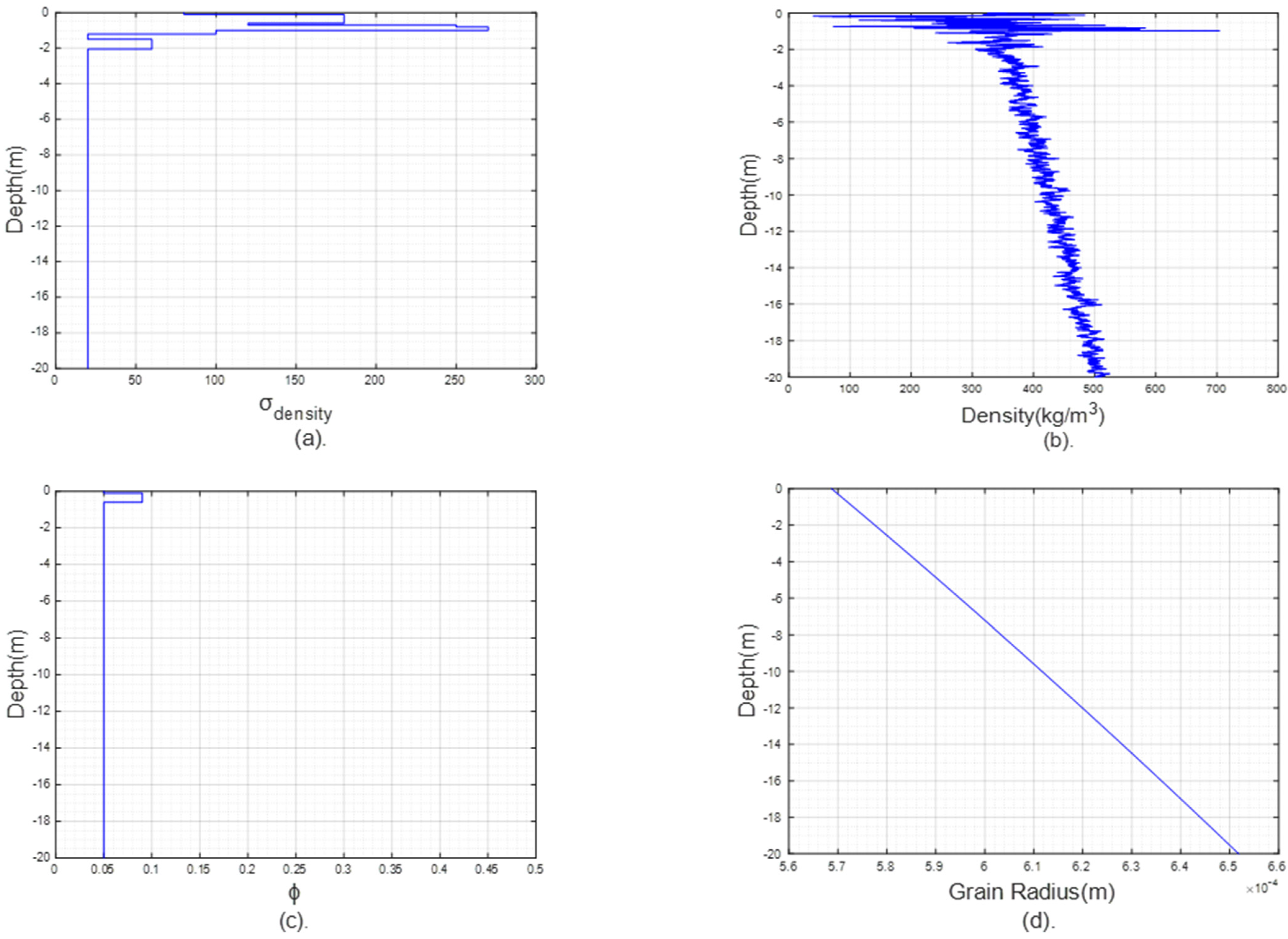
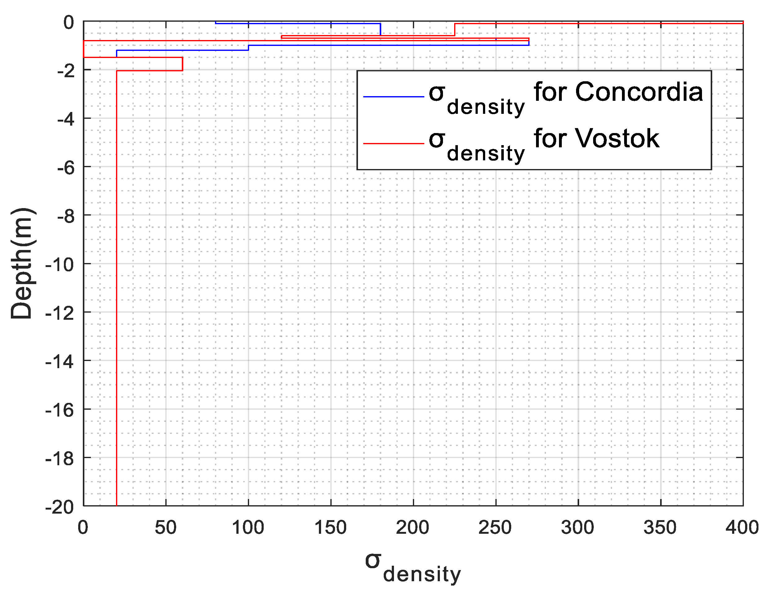
2.1.1. Firn Density
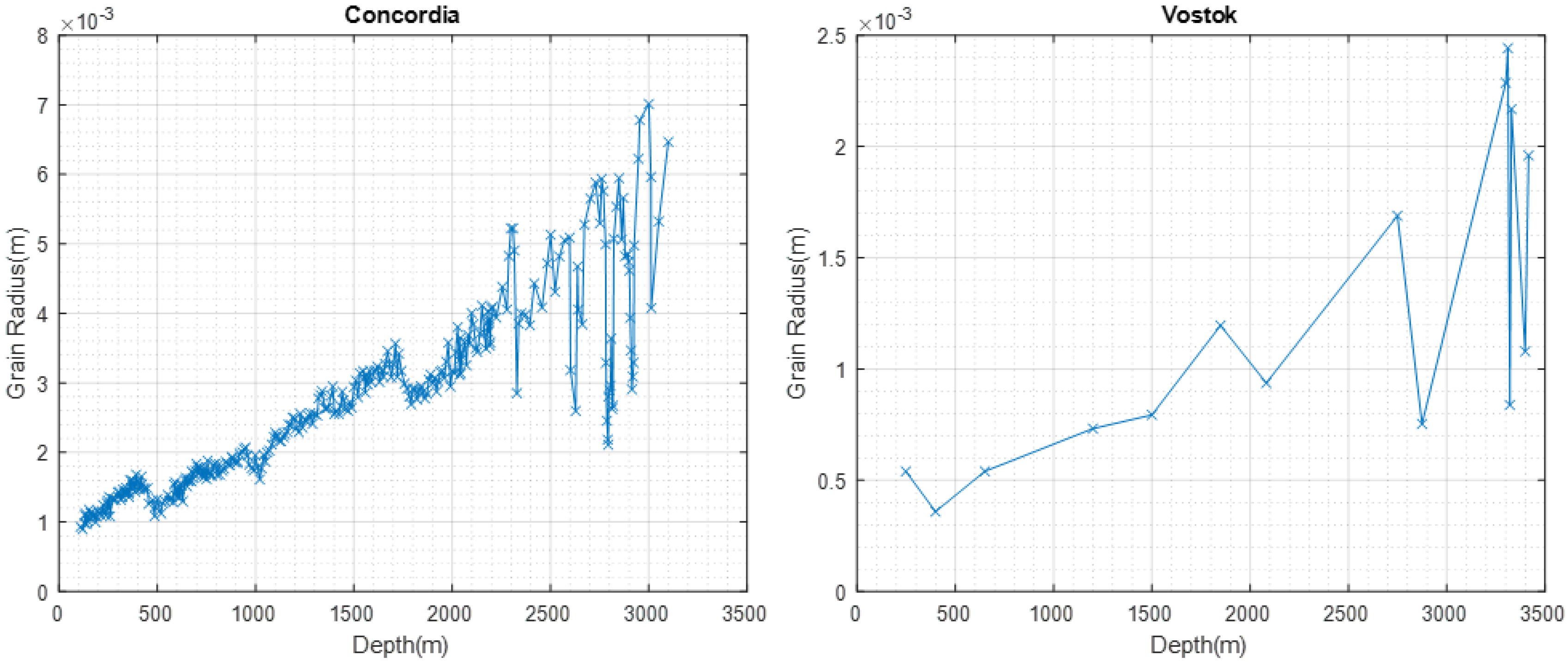
2.1.2. Grain Size
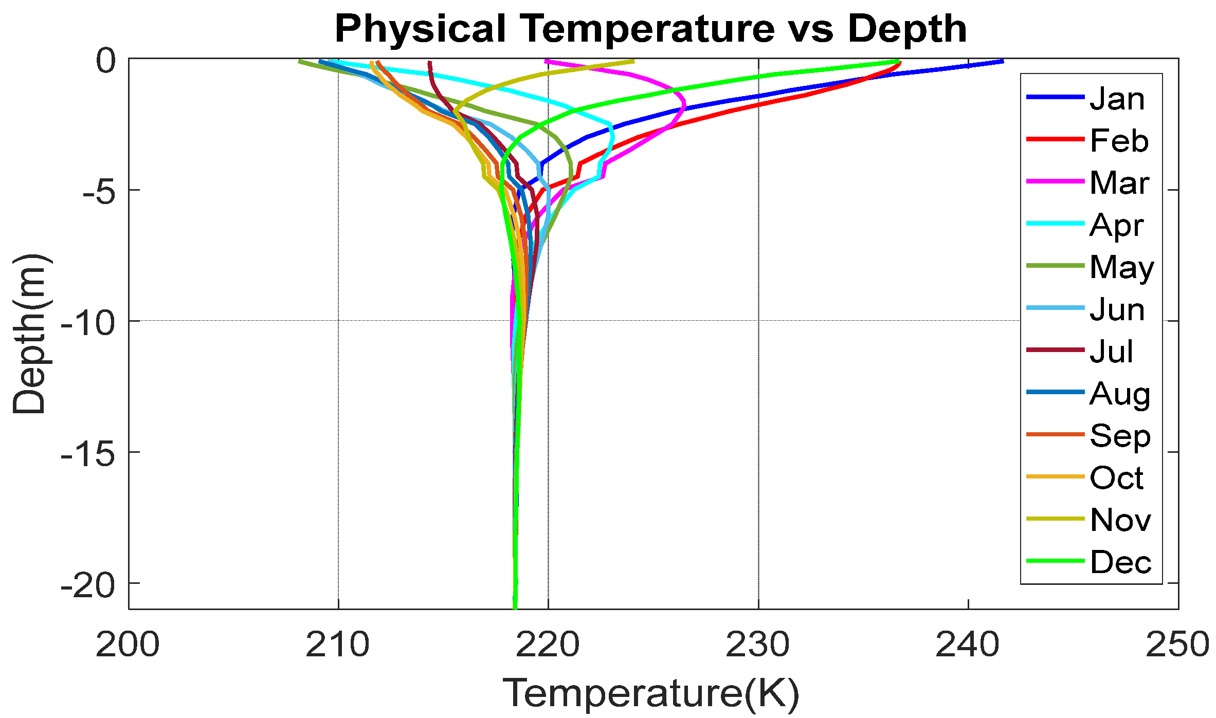
2.1.3. Firn Temperature
2.1.4. Complex Permittivity
2.1.5. Effective Permittivity
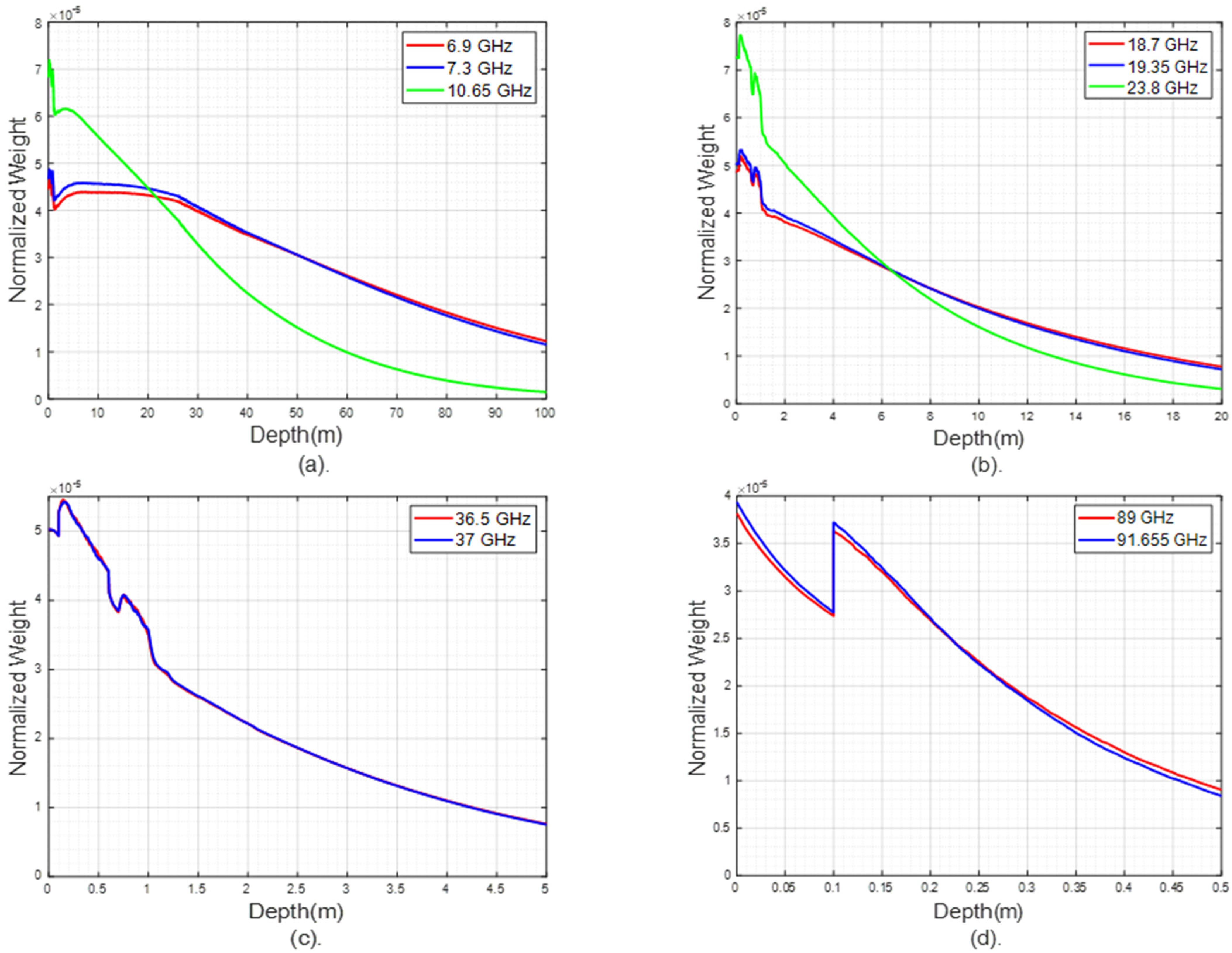
2.2. Radiation Model
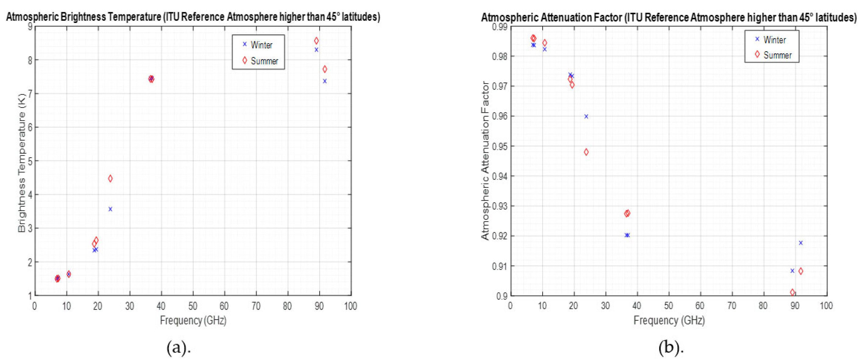
Atmospheric Attenuation
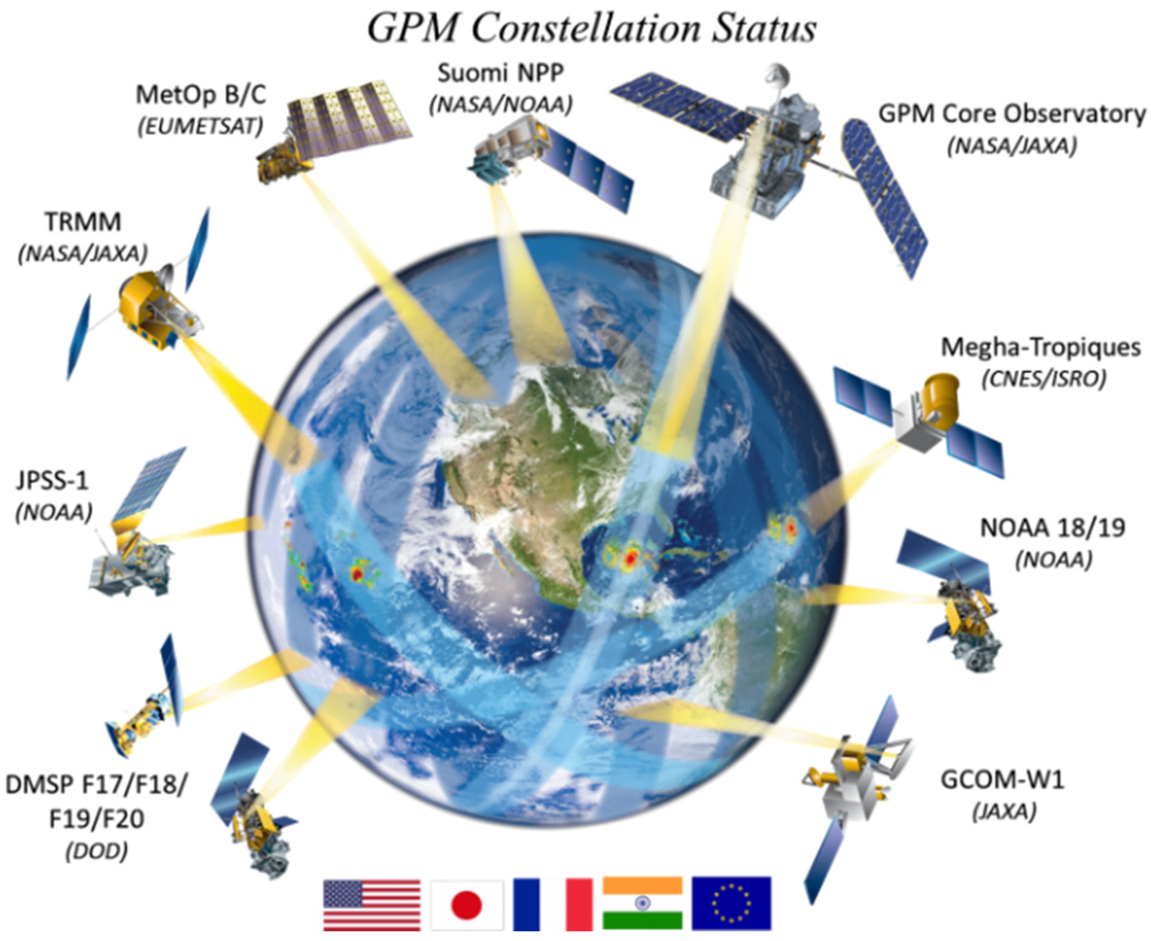
2.3. Global Precipitation Measurement Mission
2.3.1. Special Sensor Microwave Imager/Sounder (SSMIS)
2.3.2. Advanced Microwave Scanning Radiometer-2 (AMSR2)
2.3.3. Intercalibration of the GPM Constellation
3. Results
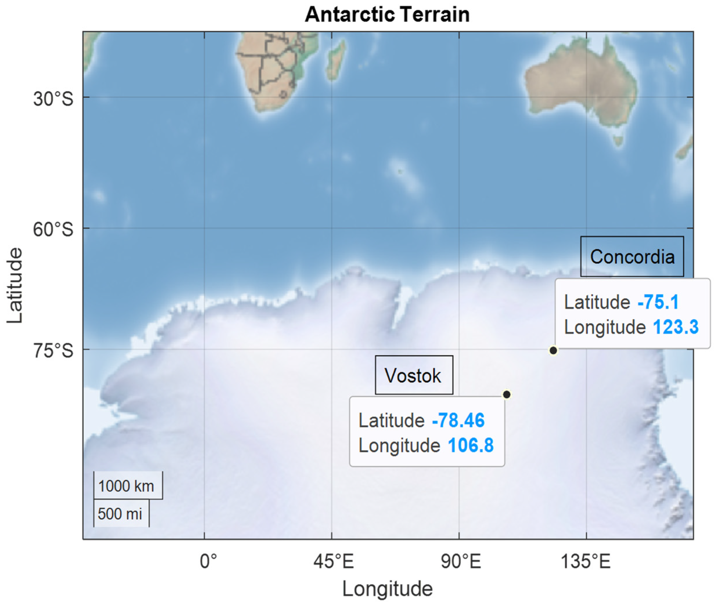
3.1. Analyses over Concordia and Vostok Stations in Antarctica
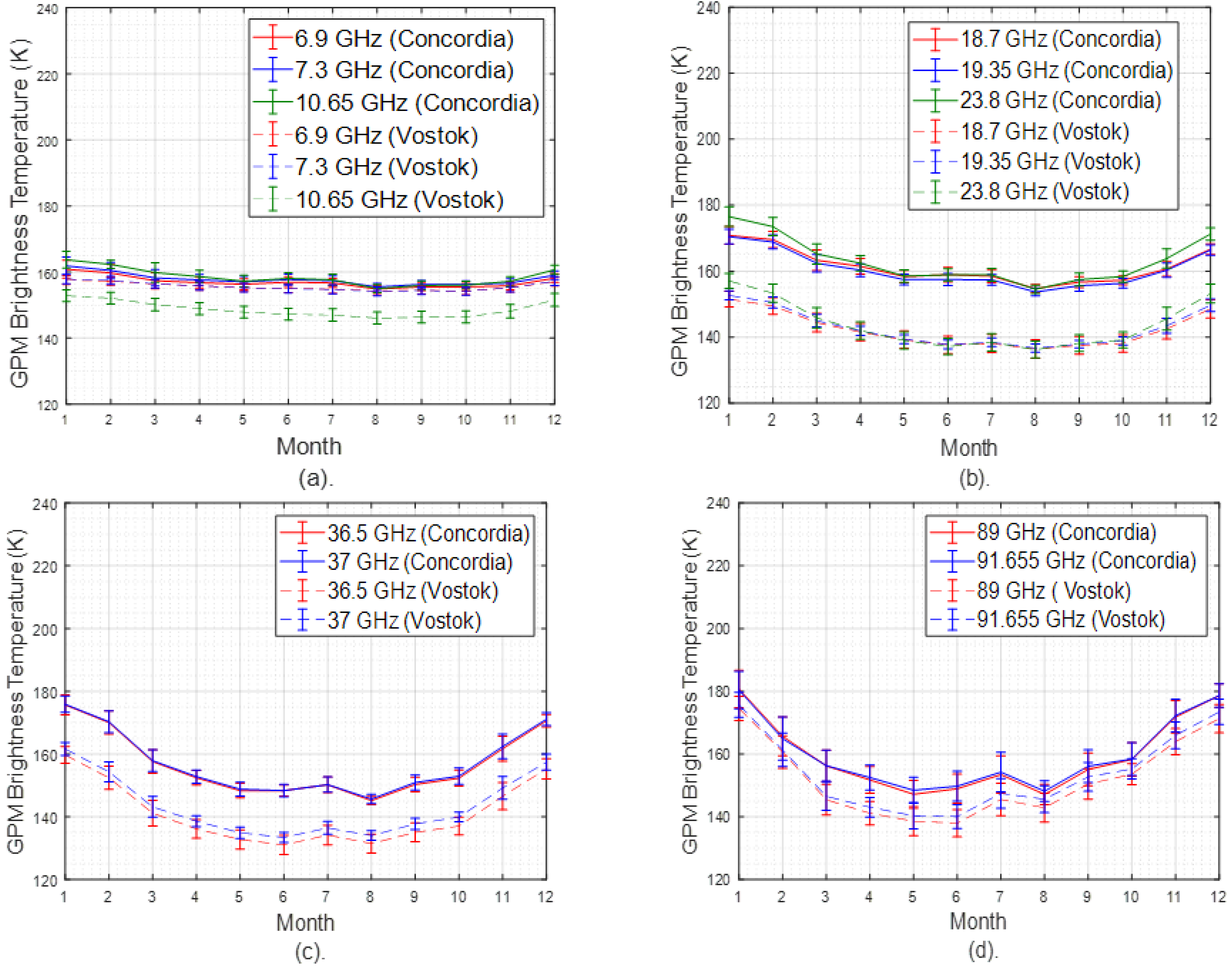
3.1.1. Satellite Measurements
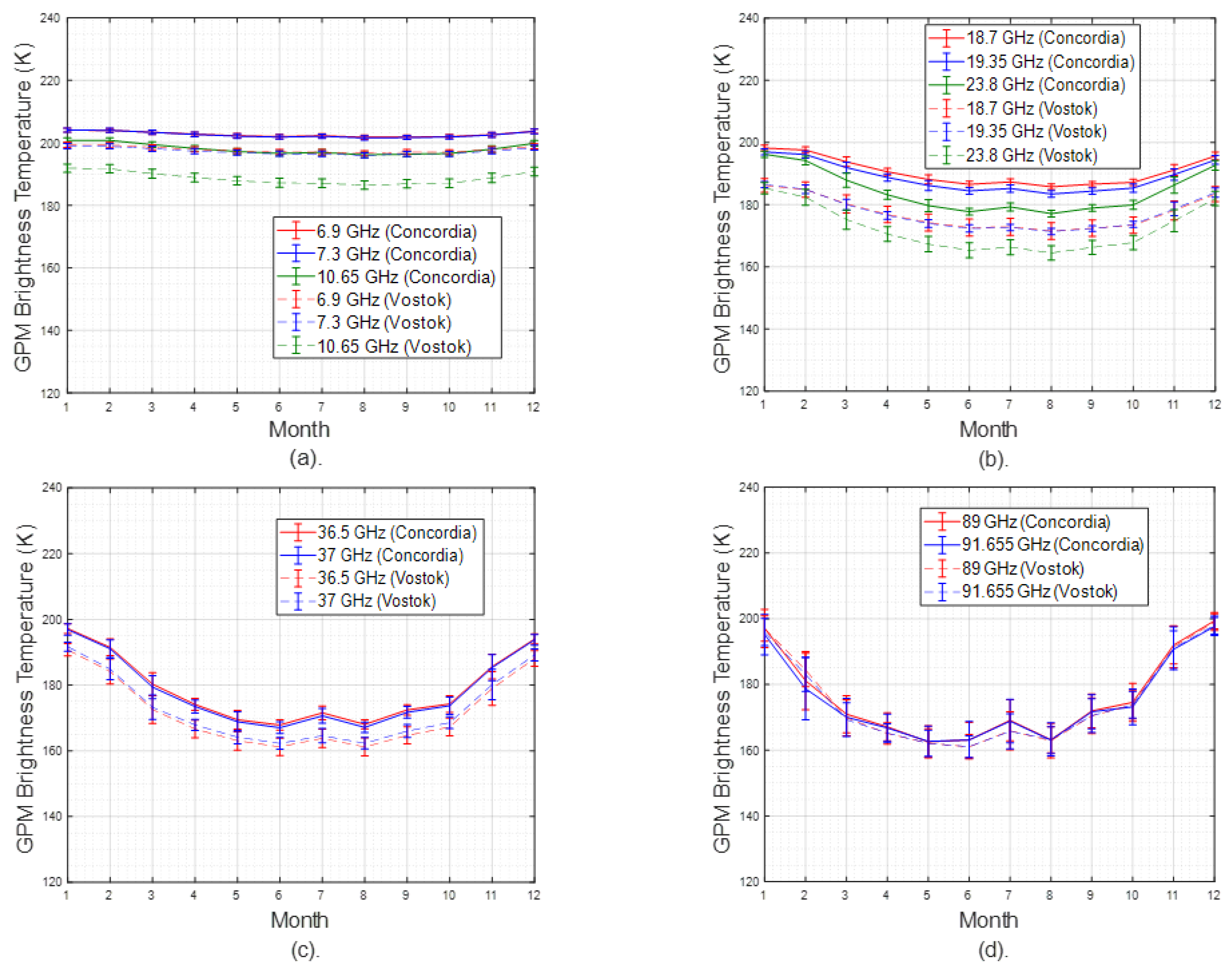
3.1.2. Radiation Simulations
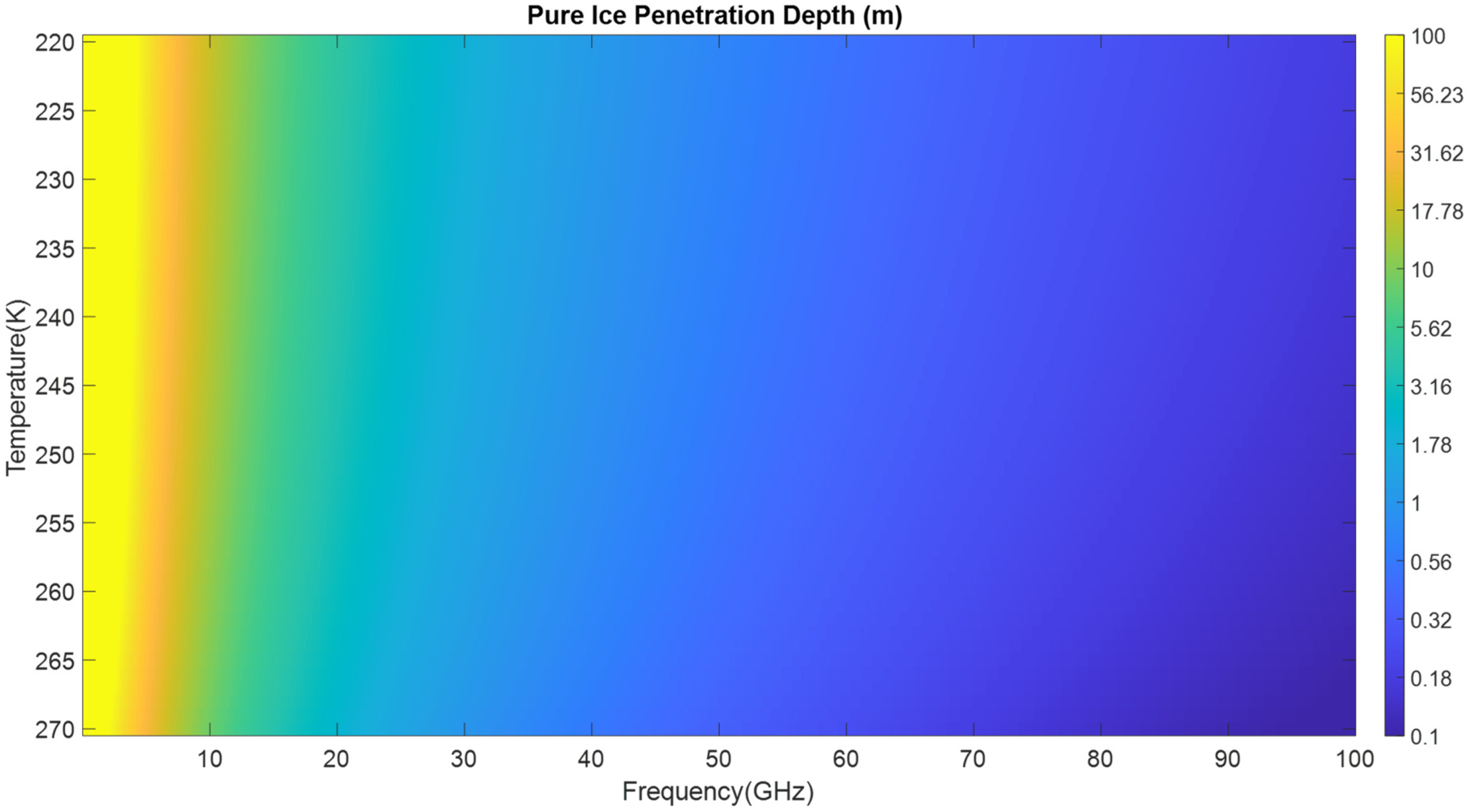
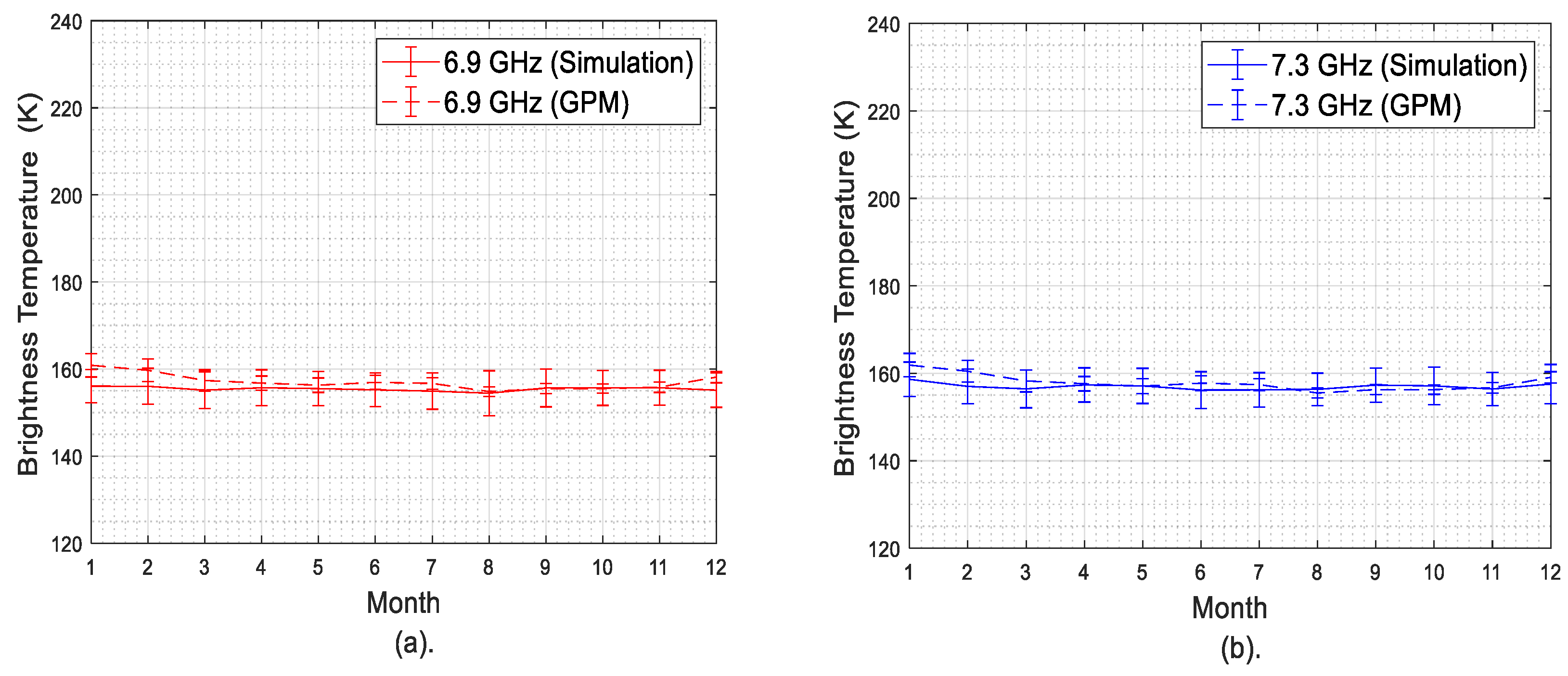
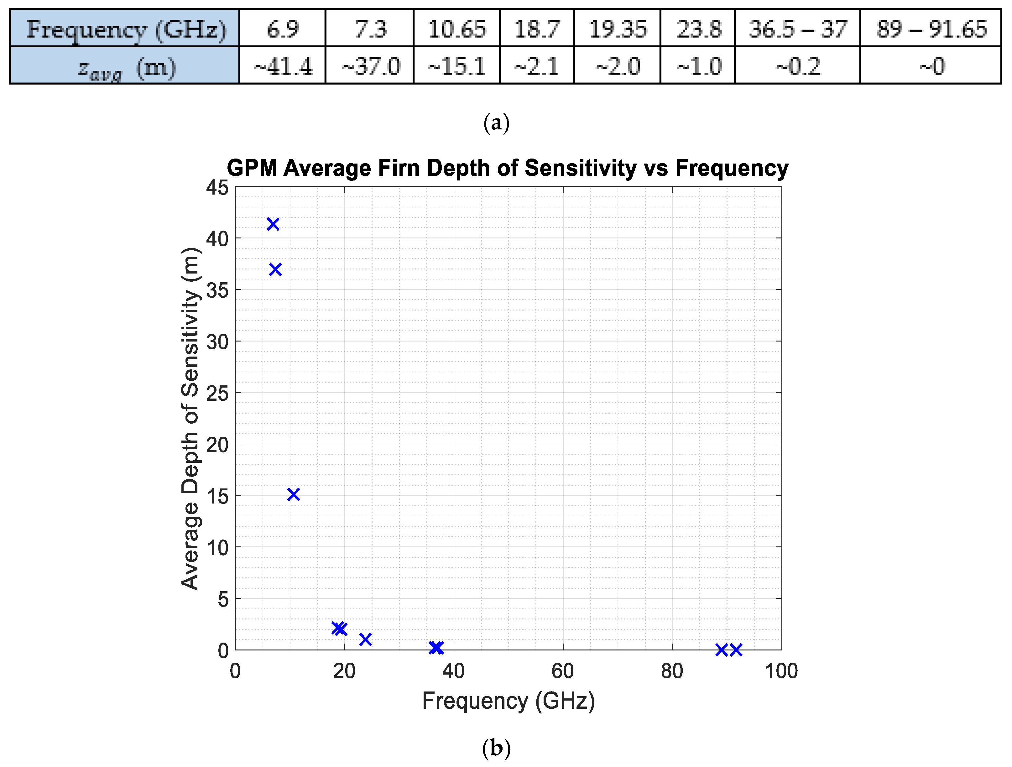
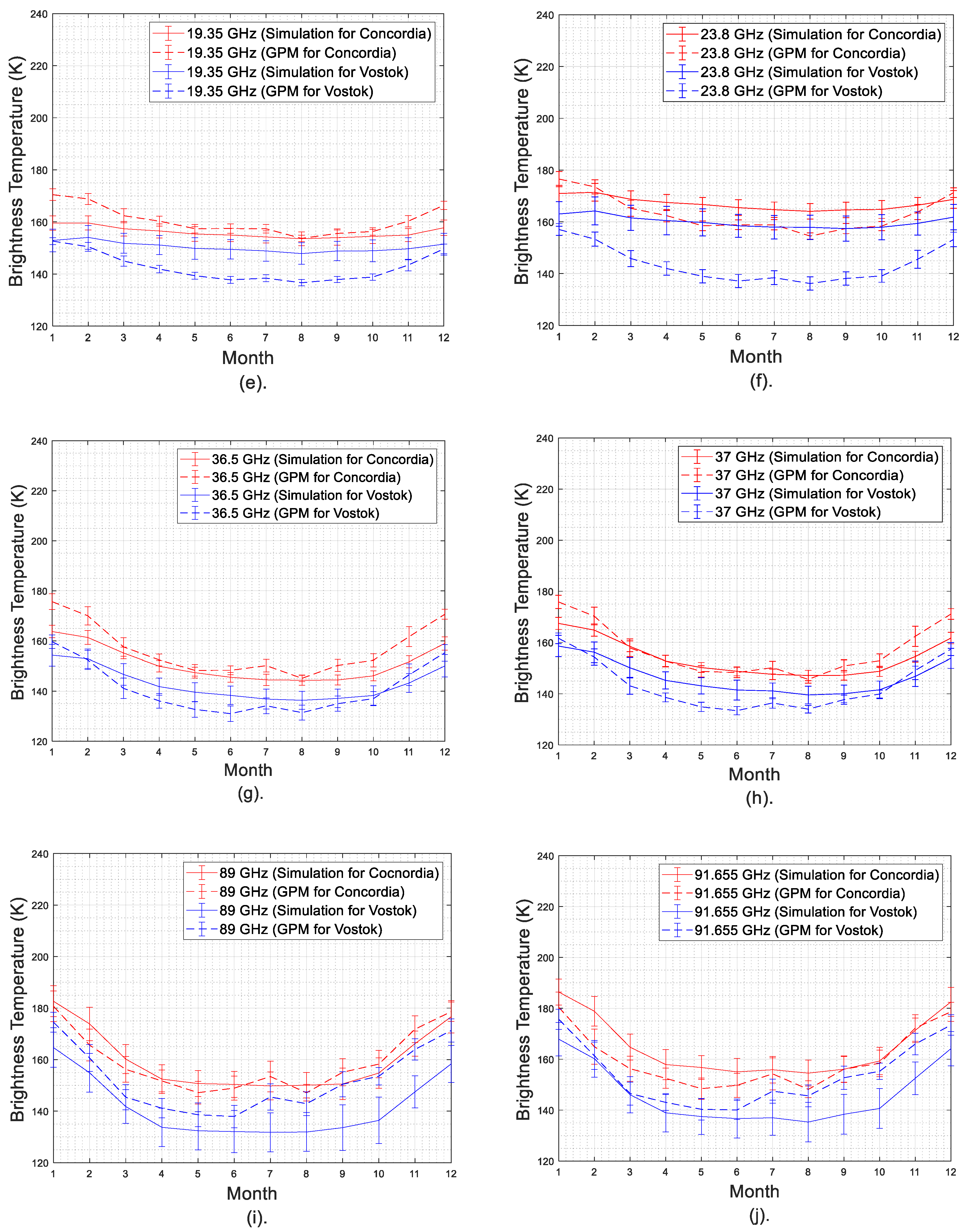
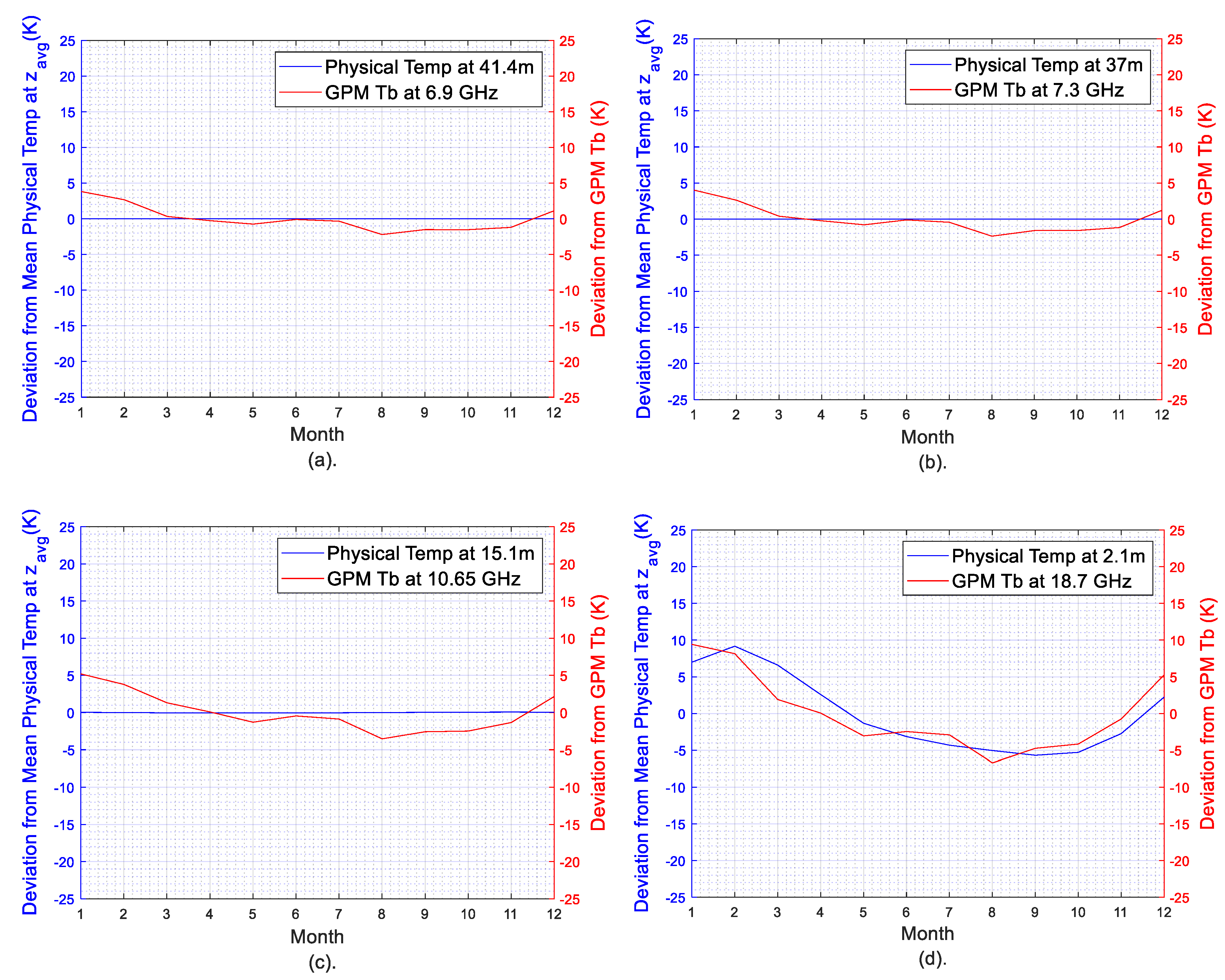
- At 6.9 GHz and 7.3 GHz, both simulated and measured brightness temperatures are almost constant during the year as expected since they are mostly sensitive to layers in isothermal deep firn, as the electromagnetic penetration depth is mostly larger than 20 m and the temperature of layers below this depth does not experience any significant seasonal variations, as shown in Figure 3 and Figure 4. Furthermore, the bias between the simulations and the measurements is negligible, as their distribution mostly overlaps throughout the year.
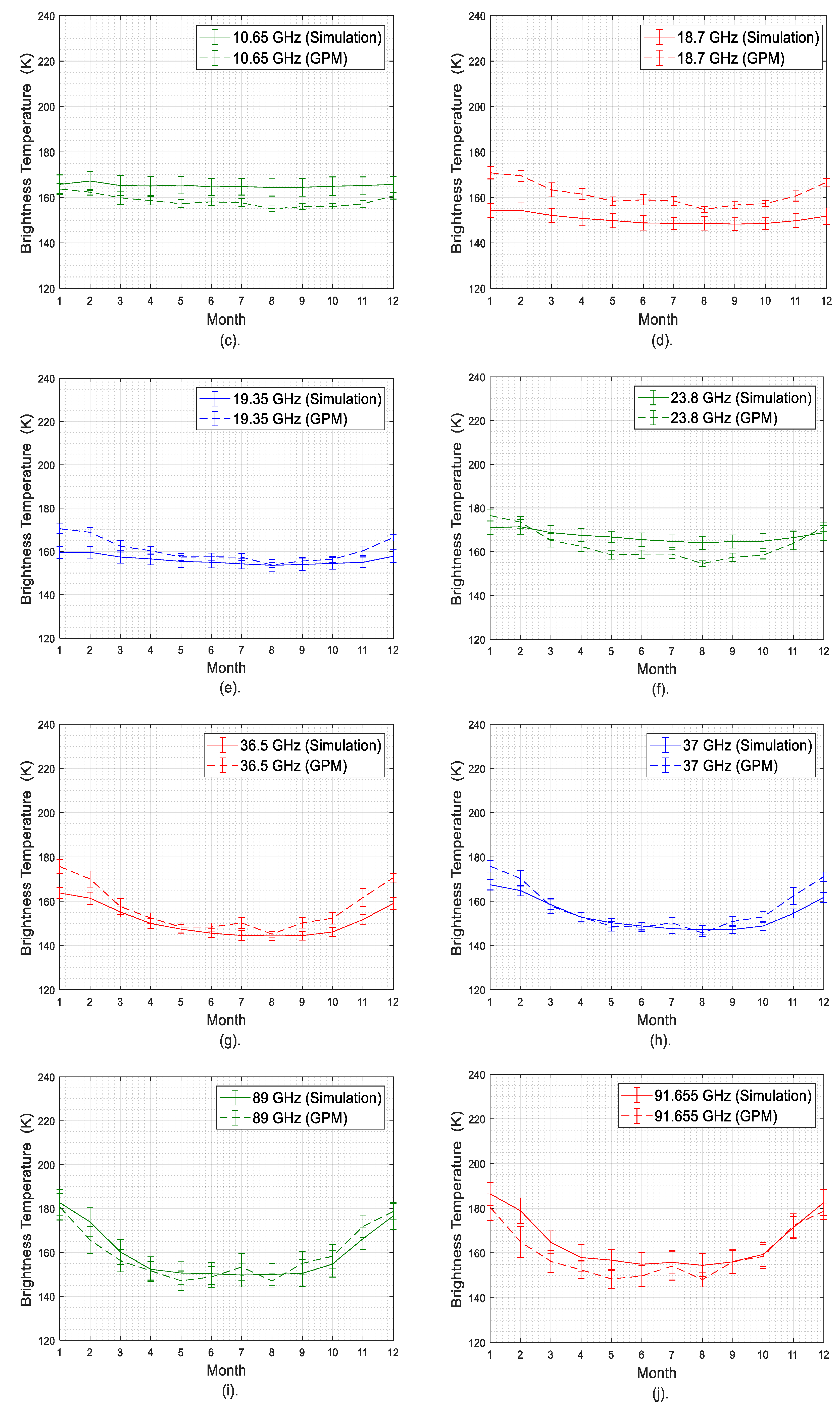
- Measured brightness temperatures exhibit 10–20 K seasonal variations at frequencies between 10.65 GHz and 23.8 GHz where the annual mean brightness temperature and the seasonal variations increase with frequency. Simulated brightness, on the other hand, underestimates these seasonal variations. Additionally, at these frequencies, biases up to 10 K have been observed in the annual mean brightness temperatures between simulations and measurements. These two sources of error have led to biases as large as 20 K, specifically at 18.7 GHz.
- Simulations and measurements at 36.5 GHz and 37 GHz agree well except in Antarctic summer (from September to March), where again, the simulations fail to follow the sharp increase in measured brightness temperatures, resulting biases up to ~10 K.
- Finally, measurements and simulations at the highest two frequencies, i.e., 89 GHz and 91.65 GHz, which exhibit the largest seasonal variations (~35 K) mostly agree with each other.
3.1.3. Retrieval Studies
3.2. Outcomes
4. Discussion
Author Contributions
Funding
Data Availability Statement
Acknowledgments
Conflicts of Interest
References
- Aksoy, M.; Johnson, J.T.; Jezek, K.C.; Durand, M.; Drinkwater, M.; Macelloni, G.; Tsang, L. An examination of multi-frequency microwave radiometry for probing subsurface ice sheet temperature. In Proceedings of the 2014 IEEE Geoscience and Remote Sensing Symposium (IGARSS), Quebec City, QC, Canada, 13–18 July 2014; pp. 3614–3617. [Google Scholar] [CrossRef]
- Solomon, S.; Manning, M.; Marquis, M.; Qin, D. Climate Change 2007—The Physical Science Basis: Working Group I Contribution to the Fourth Assessment Report of the IPCC; Cambridge University Press: Cambridge, UK, 2007; Volume 4. [Google Scholar]
- Picard, G.; Royer, A.; Arnaud, L.; Fily, M. Influence of meter-scale wind-formed features on the variability of the microwave brightness temperature around Dome C in Antarctica. Cryosphere 2014, 8, 1105–1119. [Google Scholar] [CrossRef] [Green Version]
- Turner, J.; Colwell, S.R.; Marshall, G.J.; Lachlan-Cope, T.A.; Carleton, A.M.; Jones, P.D.; Lagun, V.; Reid, P.A.; Iagovkina, S. Antarctic climate change during the last 50 years. Int. J. Climatol. 2005, 25, 279–294. [Google Scholar] [CrossRef]
- Steig, E.J.; Schneider, D.P.; Rutherford, S.D.; Mann, M.E.; Comiso, J.C.; Shindell, D.T. Warming of the Antarctic ice-sheet surface since the 1957 International Geophysical Year. Nature 2009, 457, 459. [Google Scholar] [CrossRef] [PubMed]
- Jezek, K.C.; Johnson, J.T.; Drinkwater, M.R.; Macelloni, G.; Tsang, L.; Aksoy, M.; Durand, M. Radiometric approach for estimating relative changes in intraglacier average temperature. IEEE Trans. Geosci. Remote Sens. 2014, 53, 134–143. [Google Scholar] [CrossRef]
- Johnson, J.T.; Jezek, K.C.; Aksoy, M.; Bringer, A.; Yardim, C.; Andrews, M.; Chen, C.C.; Belgiovane, D.; Leuski, V.; Durand, M.; et al. The Ultra-wideband Software-Defined Radiometer (UWBRAD) for ice sheet internal temperature sensing: Results from recent observations. In Proceedings of the 2016 IEEE Geoscience and Remote Sensing Symposium (IGARSS), Beijing, China, 10–15 July 2016; pp. 7085–7087. [Google Scholar] [CrossRef]
- Duan, Y.; Durand, M.; Jezek, K.; Yardim, C.; Bringer, A.; Aksoy, M.; Johnson, J. Testing the feasibility of a bayesian retrieval of greenland ice sheet internal temperature from ultra-wideband software-defined microwave radiometer (UWBRAD) measurements. In Proceedings of the 2016 IEEE Geoscience and Remote Sensing Symposium (IGARSS), Beijing, China, 10–15 July 2016; pp. 7092–7093. [Google Scholar] [CrossRef]
- Yardim, C.; Johnson, J.T.; Jezek, K.C.; Andrews, M.J.; Durand, M.; Duan, Y.; Tan, S.; Tsang, L.; Brogioni, M.; Macelloni, G.; et al. Greenland Ice Sheet Subsurface Temperature Estimation Using Ultrawideband Microwave Radiometry. IEEE Trans. Geosci. Remote Sens. 2022, 60, 1–12. [Google Scholar] [CrossRef]
- Andrews, M.; Johnson, J.T.; Jezek, K.; Li, H.; Bringer, A.; Chen, C.; Belgiovane, D.J.; Leuski, V.; Macelloni, G.; Brogioni, M. The Ultrawideband Software-Defined Microwave Radiometer: Instrument Description and Initial Campaign Results. IEEE Trans. Geosci. Remote Sens. 2018, 56, 5923–5935. [Google Scholar] [CrossRef]
- Fujita, S.; Goto-Azuma, K.; Hirabayashi, M.; Hori, A.; Iizuka, Y.; Motizuki, Y.; Motoyama, H.; Takahashi, K. Densification of layered firn in the ice sheet at Dome Fuji, Antarctica. J. Glaciol. 2016, 62, 103–123. [Google Scholar] [CrossRef] [Green Version]
- Herron, M.M.; Langway, C.C. Firn densification: An empirical model. J. Glaciol. 1980, 25, 373–385. [Google Scholar] [CrossRef]
- Zwally, H.J.; Giovinetto, M.B.; Li, J.; Cornejo, H.G.; Beckley, M.A.; Brenner, A.C.; Saba, J.L.; Yi, D. Mass changes of the Greenland and Antarctic ice sheets and shelves and contributions to sea-level rise: 1992–2002. J. Glaciol. 2005, 51, 509–527. [Google Scholar] [CrossRef] [Green Version]
- Alley, R.B.; Bolzan, J.F.; Whillans, I.M. Polar firn densification and grain growth. Ann. Glaciol. 1982, 3, 7–11. [Google Scholar] [CrossRef] [Green Version]
- Nye, J.F. Correction factor for accumulation measured by the thickness of the annual layers in an ice sheet. J. Glaciol. 1963, 4, 785–788. [Google Scholar] [CrossRef] [Green Version]
- Brucker, L.; Picard, G.; Arnaud, L.; Barnola, J.M.; Schneebeli, M.; Brunjail, H.; Lefebvre, E.; Fily, M. Modeling time series of microwave brightness temperature at Dome C, Antarctica, using vertically resolved snow temperature and microstructure measurements. J. Glaciol. 2011, 57, 171–182. [Google Scholar] [CrossRef] [Green Version]
- Brucker, L.; Picard, G.; Fily, M. Snow grain-size profiles deduced from microwave snow emissivities in Antarctica. J. Glaciol. 2010, 56, 514–526. [Google Scholar]
- Picard, G.; Brucker, L.; Fily, M.; Gallée, H.; Krinner, G. Modeling time series of microwave brightness temperature in Antarctica. J. Glaciol. 2009, 55, 537–551. [Google Scholar] [CrossRef] [Green Version]
- Tan, S.; Aksoy, M.; Brogioni, M.; Macelloni, G.; Durand, M.; Jezek, K.C.; Wang, T.L.; Tsang, L.; Johnson, J.T.; Drinkwater, M.R.; et al. Physical models of layered polar firn brightness temperatures from 0.5 to 2 GHz. IEEE J. Sel. Top. Appl. Earth Obs. Remote Sens. 2015, 8, 3681–3691. [Google Scholar] [CrossRef]
- Jezek, K.C.; Johnson, J.T.; Tan, S.; Tsang, L.; Andrews, M.J.; Brogioni, M.; Macelloni, G.; Durand, M.; Chen, C.C.; Belgiovane, D.J.; et al. 500–2000-MHz brightness temperature spectra of the northwestern greenland ice sheet. IEEE Trans. Geosci. Remote Sens. 2017, 56, 1485–1496. [Google Scholar] [CrossRef]
- Durand, G.; Weiss, J. EPICA Dome C Ice Cores Grain Radius Data. IGBP PAGES/World Data Center for Paleoclimatology Data Contribution Series # 2004-039; NOAA/NGDC Paleoclimatology Program: Boulder, CO, USA, 2004.
- Baker, I.; Obbard, R. Microstructural Location and Composition of Impurities in Polar Ice Cores; US Antarctic Program (USAP) Data Center: Boulder, CO, USA, 2010.
- Matzler, C.; Wegmuller, U. Dielectric properties of freshwater ice at microwave frequencies. J. Phys. D Appl. Phys. 1987, 20, 1623. [Google Scholar] [CrossRef]
- Mätzler, C. Thermal Microwave Radiation: Applications for Remote Sensing; IET: London, UK, 2006; Volume 52. [Google Scholar]
- Shih, S.E.; Ding, K.H.; Kong, J.A.; Yang, Y.E. Modeling of millimeter wave backscatter of time-varying snowcover. Prog. Electromagn. Res. 1997, 16, 305–330. [Google Scholar] [CrossRef] [Green Version]
- Tsang, L.; Kong, J.A.; Ding, K.H.; Ao, C.O. Scattering of Electromagnetic Waves: Numerical Simulations; John Wiley & Sons: Hoboken, NJ, USA, 2004; Volume 25. [Google Scholar]
- Proksch, M.; Mätzler, C.; Wiesmann, A.; Lemmetyinen, J.; Schwank, M.; Löwe, H.; Schneebeli, M. MEMLS3a: Microwave Emission Model of Layered Snowpacks adapted to include backscattering. Geosci. Model Dev. 2015, 8, 2611–2626. [Google Scholar] [CrossRef] [Green Version]
- Pan, J.; Durand, M.; Sandells, M.; Lemmetyinen, J.; Kim, E.J.; Pulliainen, J.; Kontu, A.; Derksen, C. Differences Between the HUT Snow Emission Model and MEMLS and Their Effects on Brightness Temperature Simulation. IEEE Trans. Geosci. Remote Sens. 2016, 54, 2001–2019. [Google Scholar] [CrossRef]
- Matzler, C. Relation between grain size and correlation length of snow. J. Glaciol. 2002, 48, 461–466. [Google Scholar] [CrossRef] [Green Version]
- Wiesmann, A.; Christian, M.; Weise, T. Radiometric and structural measurements of snow samples. Radio Sci. 1998, 3, 273–289. [Google Scholar] [CrossRef]
- Recommendation ITU-R P.835-6. Attenuation by Atmospheric Gases. Available online: https://www.itu.int/dms_pubrec/itu-r/rec/p/R-REC-P.835-6-201712-I!!PDF-E.pdf (accessed on 15 July 2020).
- Smith, E.A.; Asrar, G.; Furuhama, Y.; Ginati, A.; Mugnai, A.; Nakamura, K.; Adler, R.F.; Chou, M.D.; Desbois, M.; Durning, J.F.; et al. International global precipitation measurement (GPM) program and mission: An overview. In Measuring Precipitation from Space; Springer: Dordrecht, The Netherlands, 2007; pp. 611–653. [Google Scholar]
- Meet the Members of NASA’s GPM Constellation. Available online: https://www.nasa.gov/content/goddard/meet-the-members-of-nasas-gpmconstellation (accessed on 14 June 2017).
- NASA. Available online: https://pmm.nasa.gov/GPM (accessed on 18 July 2021).
- Kunkee, D.B.; Poe, G.A.; Boucher, D.J.; Swadley, S.D.; Hong, Y.; Wessel, J.E.; Uliana, E.A. Design and evaluation of the first special sensor microwave imager/sounder. IEEE Trans. Geosci. Remote Sens. 2008, 46, 863–883. [Google Scholar] [CrossRef]
- Imaoka, K.; Kachi, M.; Kasahara, M.; Ito, N.; Nakagawa, K.; Oki, T. Instrument performance and calibration of AMSR-E and AMSR2. Int. Arch. Photogramm. Remote Sens. Spat. Inf. Sci. 2010, 38, 13–18. [Google Scholar]
- Chang, P.; Jelenak, Z.; Alsweiss, S.; Sapp, J.; Meyers, P.; Ferraro, R. An overview of NOAA’s GCOM-W1/AMSR-2 product processing and utilization. In Proceedings of the 2019 IEEE Geoscience and Remote Sensing Symposium (IGARSS), Yokohama, Japan, 28 July–2 August 2019; pp. 8780–8783. [Google Scholar] [CrossRef]
- Berg, W.; Bilanow, S.; Chen, R.; Datta, S.; Draper, D.; Ebrahimi, H.; Farrar, S.; Jones, W.L.; Kroodsma, R.; McKague, D.; et al. Intercalibration of the GPM microwave radiometer constellation. J. Atmos. Ocean. Technol. 2016, 33, 2639–2654. [Google Scholar] [CrossRef]
- Precipitation Processing System. Available online: https://pps.gsfc.nasa.gov/ (accessed on 11 July 2021).
- G-Portal, Globe Portal System. Available online: https://gportal.jaxa.jp/gpr/?lang=en (accessed on 18 July 2021).
- Picard, G.; Brucker, L.; Roy, A.; Dupont, F.; Fily, M.; Royer, A. Simulation of the microwave emission of multi-layered snowpacks using the dense media radiative transfer theory: The DMRT-ML model. Geosci. Model Dev. Discuss. 2012, 5, 3647–3694. [Google Scholar] [CrossRef] [Green Version]
- Entekhabi, D.; Eni, G.N.; Peggy, E.N.; Kent, H.K.; Wade, T.C.; Edelstein, W.N.; Entin, J.K.; Goodman, S.D.; Jackson, T.J.; Johnson, J.; et al. The soil moisture active passive (SMAP) mission. Proc. IEEE 2010, 98, 704–716. [Google Scholar] [CrossRef]


Publisher’s Note: MDPI stays neutral with regard to jurisdictional claims in published maps and institutional affiliations. |
© 2022 by the authors. Licensee MDPI, Basel, Switzerland. This article is an open access article distributed under the terms and conditions of the Creative Commons Attribution (CC BY) license (https://creativecommons.org/licenses/by/4.0/).
Share and Cite
Kar, R.; Aksoy, M.; Kaurejo, D.; Atrey, P.; Devadason, J.A. Antarctic Firn Characterization via Wideband Microwave Radiometry. Remote Sens. 2022, 14, 2258. https://doi.org/10.3390/rs14092258
Kar R, Aksoy M, Kaurejo D, Atrey P, Devadason JA. Antarctic Firn Characterization via Wideband Microwave Radiometry. Remote Sensing. 2022; 14(9):2258. https://doi.org/10.3390/rs14092258
Chicago/Turabian StyleKar, Rahul, Mustafa Aksoy, Dua Kaurejo, Pranjal Atrey, and Jerusha Ashlin Devadason. 2022. "Antarctic Firn Characterization via Wideband Microwave Radiometry" Remote Sensing 14, no. 9: 2258. https://doi.org/10.3390/rs14092258