1. Introduction
Light detection and ranging (LiDAR) can obtain real three-dimensional spatial coordinate information within the measurement range [
1]. This has the characteristics of high efficiency and high accuracy. LiDAR is widely used in urban planning, agricultural development, environmental monitoring, and transportation [
2]. Ground filtering is a key technology to separate and extract ground information from the point-cloud data obtained by LiDAR [
3,
4]. Point cloud filtering is a significant step in the process of point-cloud processing [
5]. Therefore, in the past two decades, scholars have proposed many effective automatic filtering algorithms, which greatly reduce the labor costs and improve the application efficiency of point-cloud data [
2]. There are many widely used methods that are well suited for different situations. However, these methods can still be better optimized.
With the development of deep-learning technology [
6], 3D-object-detection methods based on convolutional neural networks have achieved high accuracy and efficiency and have been gradually applied in the fields of autonomous driving and robotics. For 3D-object detection, many scholars have proposed network structures, and these networks have superior performance [
7,
8,
9]. Commonly used methods for 3D-object detection include converting point clouds into voxels [
10] and pseudo images [
11]. This also includes PointRCNN [
12], which processes point clouds directly. Research progress has also been made in joint 3D-instance segmentation and object detection [
13].
However, the general practice of the current 3D-object detection algorithm is to directly process the collected point cloud, and few scholars have considered removing the ground first. The main reason is that the accuracy and efficiency of the current ground filtering algorithms have difficulty in meeting the application requirements of 3D-object detection. For example, the ground filtering accuracy is insufficient, which will result in part of the ground being retained and some objects being removed. This will seriously affect the object detection accuracy. At the same time, computational efficiency is an important indicator of 3D-object detection. If the ground filtering efficiency is insufficient, it is also impossible to be applied. Therefore, a fast and high-precision ground filtering method is currently needed.
Since the elevation changes of most scenes are relatively small, many researchers treat the ground surface as a flat surface [
14]. Fan et al. builds a plane function by using RANSAC. The ground points whose distance to the optimal plane is within the threshold are recognized [
15]. When the ground is uneven, this method has obvious defects. In order to improve the fitting accuracy in large scenes, Golovinskiy filters out the ground points locally [
16].
As the whole ground cannot be a flat plane. Part of the ground is mostly a flat plane. However, they only filter the ground points through the plane fitting method and do not consider the problems that may be caused by the local plane fitting. Similarly, this paper uses a local method to filter out the ground points. The proposed method first divides the point cloud into several blocks, which is essential to obtain a local point cloud. This paper analyzes the problems that may be caused by local ground fitting, and proposes effective solutions.
For the efficiency and accuracy of RANSAC, Universal-RANSAC [
17] conducted a detailed analysis and proposed a comprehensive solution. Similarly, we analyze the steps of RANSAC in detail and optimize the two key steps of sampling and determining the optimal plane, respectively.
Sampling: RANSAC uses a completely random approach. The premise of this approach is that we have absolutely no idea what the data is like. However, in practical applications, prior knowledge of the data is known. GroupSAC [
18] considers points within a class to be more similar, and points in a dataset are grouped according to some similarity. Sampling starts with the largest cluster as there should be a higher proportion of inliers here. In the process of LiDAR ground filtering, the heights of the two adjacent parts of the ground are essentially the same, and thus we can first estimate the height of the ground and set constraints. Our scheme can also deal with the problems caused by local ground fitting.
Determining the optimal plane: After RANSAC calculates the model, the number of points that satisfy the parameters in all sets is calculated. Preemptive RANSAC [
19] first generates multiple models, and then a selected subset is used to rank the generated models according to the objective function score. The first few are selected, and several rounds of similar sorting are performed to select the best model. We also adopt this idea. Multiple models are generated, and the best one is selected. This avoids multiple iterations and improves the efficiency.
The contributions of this article are as follows.
We propose an improved RANSAC. We analyze the principle of GroupSAC, design the sampling method and effectively solve the problems that may be caused by local point cloud filtering. We analyze Preemptive RANSAC and devise a method for determining the optimal plane. Based on these two key steps of RANSAC, a LiDAR ground filtering method is proposed.
We experimentally verify that the accuracy and efficiency of the proposed method are higher than the current commonly used methods. The filtering results obtained by the proposed method can better preserve the details in the point cloud.
We explore the application of point cloud filtering methods to 3D-object detection. The proposed method can improve the accuracy of 3D-object detection to a certain extent without affecting the efficiency.
2. Related Work
2.1. LiDAR Filtering
In recent years, researchers have proposed a variety of ground filtering algorithms, which can be classified according to different criteria. For example, filtering algorithms can be divided into urban pavement and wild vegetation according to the ground type. According to the processing method, these can be divided into single-step filtering and iterative filtering. After sorting out the ground filtering algorithms, the current mainstream algorithms are divided into three categories according to the point-cloud division and processing methods. These are the ground filtering algorithm based on morphology, the ground filtering algorithm based on space division and the ground filtering algorithm based on iterative least square interpolation.
Morphological filtering was the earliest filtering algorithm applied to LiDAR. The specific steps of this method are to divide the point-cloud data into grids, and the grid elevation information is used to erode the non-ground points to extract the ground points [
20]. The progressive morphological filter gradually increases the window size, and according to the window size, the elevation difference threshold information is used to retain ground points and remove points from non-ground objects [
21].
Pirotti used a multi-dimensional grid to apply a progressive morphological filter to remove non-ground points [
22]. The algorithm does not require multiple iterations and can optimize the speed; however, it relies heavily on reflectance information. Trepekli evaluated the performance of morphological filter, and the results show that the performance of morphological filter on uniform surface is satisfactory [
23].
This method generally requires interpolation and gridding before data processing, which will cause damage to the original terrain features. Furthermore, this kind of method only uses the lowest point of the window as the ground point. Assuming that the roof area is large and the ground is not included in the window, there will be errors in the filtering results, and this method is not applicable. In addition, the size of the structural window and the setting of the elevation threshold are the main factors that affect this filtering. This also leads to the impracticality of these methods.
Ground filtering based on space division is a mixture of grid-based filtering and three-dimensional voxel-based filtering. The grid-based filtering is to grid the horizontal plane of the point cloud space. Thrun et al. proposed a filtering algorithm based on the minimum–maximum height difference [
24]. The ground filtering based on a two-dimensional grid uses local ground information instead of global continuity information for filtering. This method is susceptible to noise or external calibration of the sensor, and thus the performance is not stable.
Three-dimensional voxels are based on a plane grid and divide the three-dimensional space into several sets according to the elevation information of the point cloud [
25]. This type of algorithm generally distinguishes ground voxels from non-ground voxels by judging the average height or variance value of the points within the voxels [
26].
The filtering method based on iterative linear least squares interpolation was first proposed by Kraus et al. [
27]. This method can obtain the terrain surface well; however, the obvious drawback of this method is that the filtering parameters need to be constantly adjusted to adapt to different types of terrain. Koebler proposed a layered robust linear interpolation method based on least squares [
28]. This method is suitable for steep areas and forest areas. Qin proposed a region growth filtering based on moving-window weighted iterative least squares fitting [
29]. This method can effectively remove buildings and vegetation; however, it still requires further improvement for the removal of bridges and objects at the edge.
Gao used least squares interpolation in the framework of road extraction to restore the elevation information of the blocked sections of the overpass [
30]. This type of algorithm needs to satisfy two conditions. First, the lowest point of elevation value within a certain area must be a ground point. Second, the distribution of ground points conforms to the quadratic surface distribution, and other points are higher than the surface. In short, the application of ground filtering methods based on least squares is limited.
2.2. RANSAC
The goal of classic RANSAC [
31] is to continuously attempt different target space parameters to maximize the objective function. This is a random, data-driven process. The estimated model is generated by iteratively randomly selecting a subspace of the dataset. The estimated model is then leveraged and tested with the remaining points in the dataset to obtain a score. Finally, the estimated model with the highest score is returned as the model for the entire dataset. Classical RANSAC has three main limitations, namely efficiency, accuracy, and degradation. There are many improvements to these limitations of the classical approach.
Under the condition of prior knowledge, the minimum subset sampling method can effectively reduce the sampling times. The main idea of NAPSAC [
32] is to regard the n-dimensional space of the dataset as a hypersphere, and as the radius decreases, the outliers decrease faster than the inliers. PROSAC [
33] uses the result of matching the initial set of points as the basis for sorting, and thus that the samples that are most likely to obtain the best parameters will appear earlier, which improves the speed. Similar to NAPSAC, the classical algorithm begins to calculate the parameters after the sampling is completed, while some algorithms verify whether the sampling results are suitable for the parameter calculation after the sampling is completed.
The model calculation is to calculate the parameters according to the minimum set selected in the previous step to obtain the model. Prior knowledge is used for model validation, such as matching point sets with circles. When verifying, it is not necessary to verify all the points in the dataset but only to verify within a radius of the model.
The verification parameter is to calculate the number of points satisfying the parameter in all sets after obtaining the parameters generated by the minimum set.
test selects d points that are much smaller than the data set as the test. Only when these d points are all in-class points, are the remaining points are tested; otherwise, the current model is discarded. The Bail-Out test [
34] selects several points in the set for testing. If the proportion of inliers is significantly lower than the proportion of inliers in the current best model, the model is discarded. The SPRT test [
35,
36] randomly selects a point and calculates the probability of conforming to the current model and the probability of not conforming. When the probability ratio exceeds a certain threshold, the current model is discarded.
The final converged RANSAC result may be affected by noise and is not the globally optimal result. This effect requires the addition of a post-processing of model refinement. When the current optimal result appears in the iterative process, Lo-RANSAC [
37] resamples from the inliers of the returned result to calculate the model by setting a fixed number of iterations and then selecting the optimal local result as the improved result. The idea of the error propagation method [
38] is consistent with Lo-RANSAC, since the initial RANSAC results are generated from a noisy dataset, and thus this error propagates to the final model.
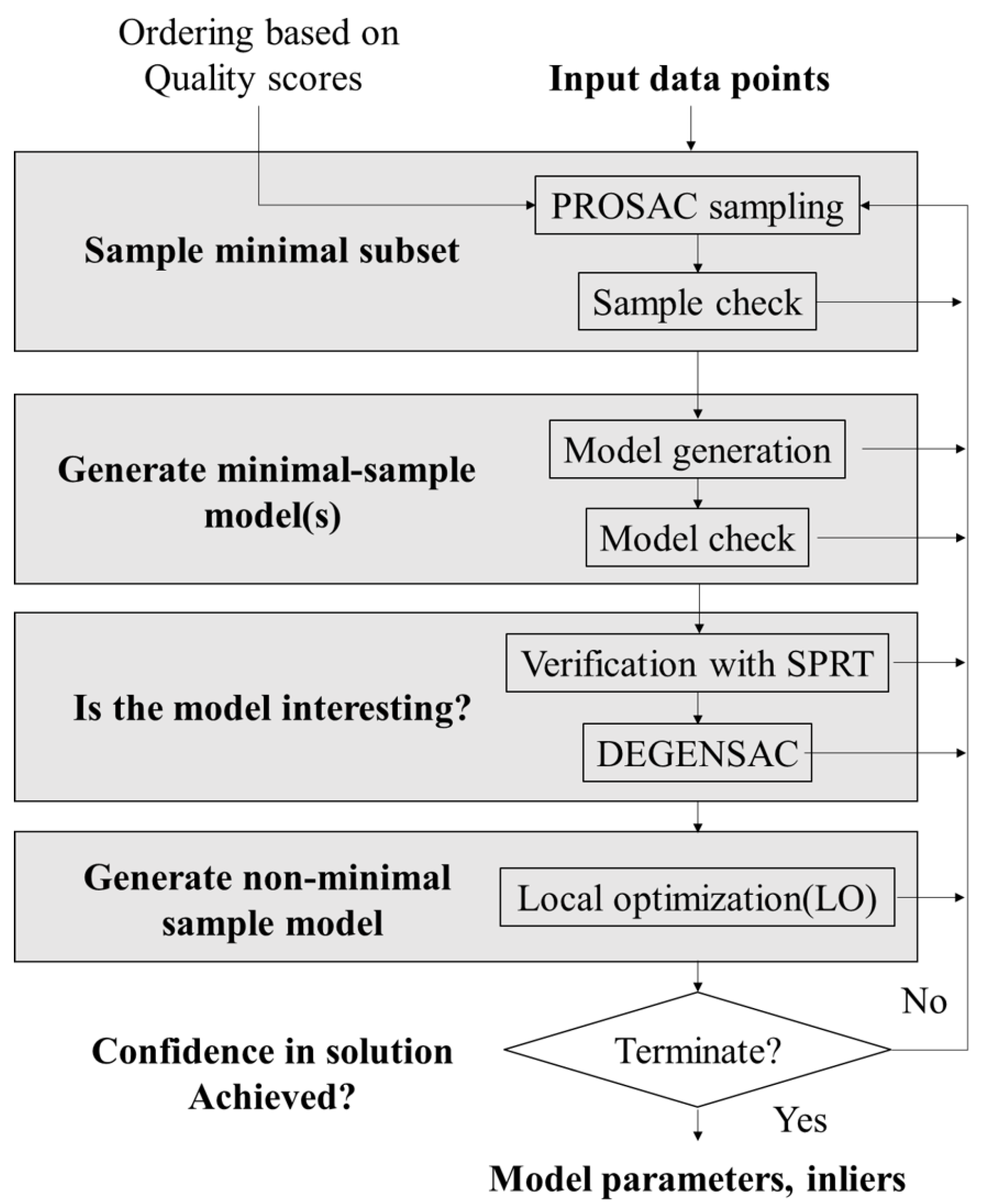
Universal-RANSAC [
17] analyzes and compares various methods to optimize the key steps of RANSAC. The algorithm flow chart of Universal-RANSAC is shown in
Figure 1. Its minimum sampling method adopts PROSAC, its model verification adopts SPRT test, and its detail optimization adopts Lo-RANSAC. In this paper, the key steps of RANSAC are optimized according to the characteristics of point clouds, and an efficient and robust LiDAR filtering method is proposed.
2.3. 3D Object Detection
3D-object detection in urban environments is a challenge, requiring the real-time detection of moving objects, such as vehicles and pedestrians. In order to realize real-time detection in large-scale point clouds, researchers have proposed a variety of methods for different requirements.
Lang et al. proposed the encoder PointPillars to learn the point-cloud representation in pillars [
11]. By operating the pillar, there is no need to manually adjust the combination of points in the vertical direction. Since all key operations can be represented as 2D convolutions, end-to-end 3D point cloud learning can be achieved using only 2D convolutions. The point cloud information can be effectively utilized by this method, and the calculation speed is fast.
Shi et al. proposed PointRCNN to generate ground-truth segmentation masks from point clouds in the scene based on bounding boxes [
12]. A small number of high-quality bounding box preselection results are generated while segmenting the foreground points. Preselected results are optimized in standard coordinates to obtain the final inspection results.
Considering the generality of the model, Yang et al. proposed STD [
39]. Spherical anchors are exploited to generate accurate predictions that retain sufficient contextual information. The normalized coordinates generated by PointPool make the model robust under geometric changes. The box prediction network eliminates the difference between localization accuracy and classification score, which can effectively improve the performance.
Liu et al. proposed LPD-Net (large-scale place description network) [
40]. The network uses an adaptive local feature extraction method to obtain the local features of the point cloud. Second, the fusion of feature space and Cartesian space can further reveal the spatial distribution of local features and learn the structural information of the entire point cloud inductively.
Zhang et al. proposed PCAN to obtain local point features and generate an attention map [
41]. The network uses ball queries of different radii to aggregate the textual feature information of points. This method can learn important point cloud features.
To overcome the limitation of the small size of point clouds in general networks, Paigwar et al. proposed Attentional PointNet [
42] using the Attentional mechanism to focus on objects of interest in large-scale and disorganized environments. However, the preprocessing step of this method makes it computationally expensive.
Voxel CNN is adopted for voxel feature learning and precise location generation to save subsequent computation and encode representative scene features [
43]. Features are then extracted, and the aggregated features can be jointly used for subsequent confidence predictions. This method combines the advantages of voxel and Pointnet to learn more accurate point cloud features.
3. LiDAR Ground Filtering
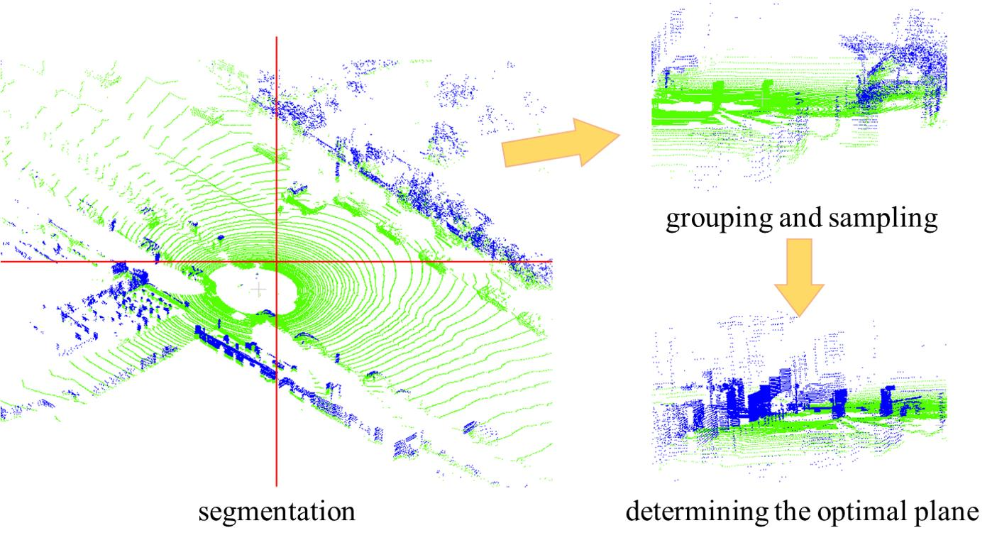
In this section, we introduce the proposed method. The sampling part is introduced first. We first analyze the principle of GroupSAC and the possible problems caused by point cloud segmentation, and based on this, we propose a method to constrain the sampled points. Then, the calculation method of the plane equation and the method of counting the number of points in the plane are introduced. Finally, based on the analysis of Preemptive RANSAC, a method to determine the optimal plane is proposed.
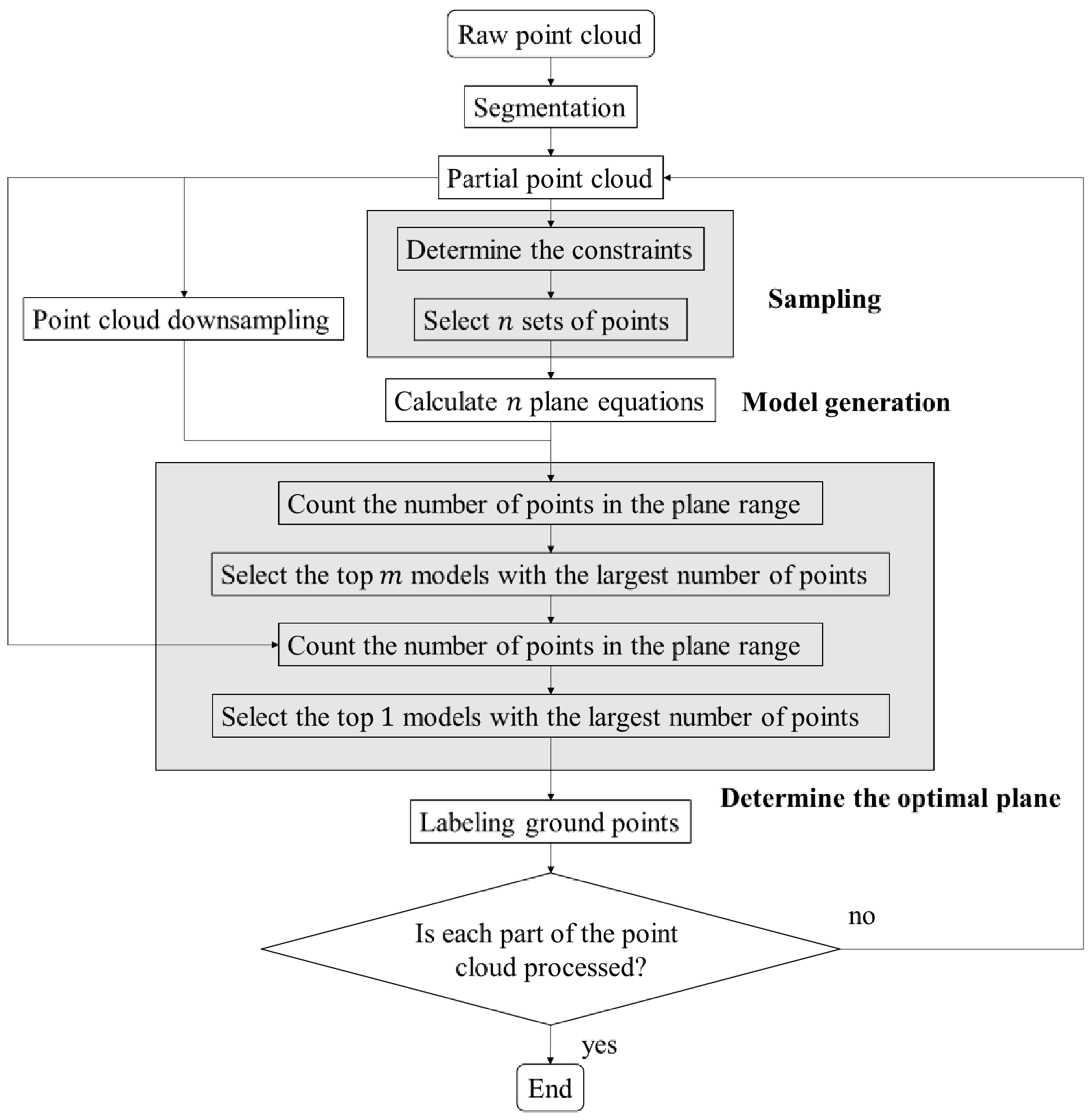
The flow chart is shown in
Figure 2. First, the point cloud is observed and divided into several parts evenly according to the length and width. We determine the constraints and select
n sets of points.
n plane equation models are built, and the point cloud is downsampled. Then, we count the number of points within the range of each plane model, and select the top
m models with the largest number of point clouds. The point cloud before downsampling is used to count the number of points within the plane model again. At this time, the selected plane model with the largest number of points is the optimal model. This process is repeated to obtain the ground model of the entire point cloud.
3.1. Sampling
3.1.1. Principle Analysis of GroupSAC
In the original RANSAC and its many improved methods, the probability that point
x is the target point in the random point sampling process obeys a Bernoulli distribution. That is, the possibility that a point is an inlier is considered to be independent of the other points. In the original RANSAC, the parameter estimation problem for an existing model from N data
is corrupted by interference. We suppose that the least number of data required for calculating the parameters of the model is
m. For any minimal data set
S with
m data:
where
is the number of all target points in
S.
is the binomial distribution. “∼” is the sign that
obeys the binomial distribution.
is the parameter of the Bernoulli trial—that is, the target point possibility of
S. Therefore, for the probability
that all data in
S are target points, the formula is:
where
is a variable indicating that
is the target point. Despite the fact that many previous works consider that
is not necessarily identical for various points. Furthermore, this inhomogeneous attribute is used to accelerate the sampling process. The target point probabilities of various points in these methods are still assumed to be independent of each other.
For many problems, there is a grouping between data. These grouped attributes tend to have high or low proportions of target points.
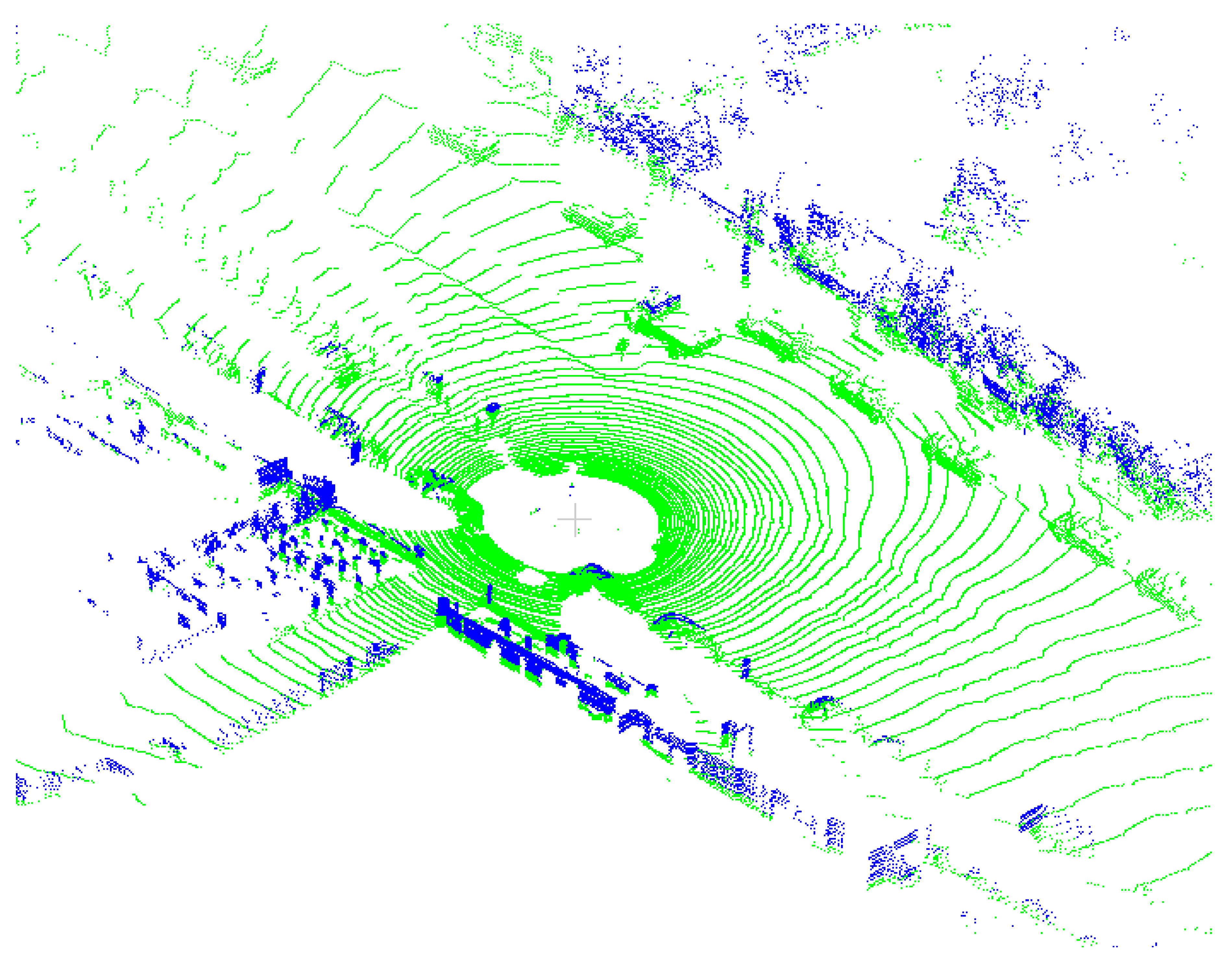
Figure 3 is used as an example. We label the point cloud with different colors based on height. We can consider a group of similar colors as a point group. The green group is more likely to contain inliers than the blue group.
We hypothesize that the probability of inliers in these sets can be modeled by a two-class compound. They are the high inlier class and the low inlier class, respectively. The characteristic of the model is that the more data in the high inlier class, the lower the inlier ratio. The inlier ratio is about 0 in the low inlier class. The delta function is also called a generalized function. The larger the range of the function’s definition domain, the smaller the range of the value domain. The value outside the domain is 0. The characteristics of the delta function are highly compatible with the model. Thus, we use the delta function for modeling. The inlier ratio
in any existing group
is:
where
and
are the mixture weights for the high inlier class and the zero inlier class. The inlier ratios of these two classes are
and 0, respectively. Therefore, the probability of having
inliers in
can be deduced as:
That is to say, the distribution of inliers
for any existing group is:
where
is the number of points in
. Therefore, inliers are generated by only a part
of the groups, called the inlier groups [
18]. In summary, we designed a method suitable for point clouds. Point clouds are grouped by height in order to find more suitable points.
3.1.2. Point Cloud Segmentation and Problem Description
We observe the horizontal and vertical slopes of the ground in the point-cloud data and make the ground of each part of the point cloud as plane as possible. The number of parts of the point cloud is as small as possible. Two problems may arise after the point cloud is divided into parts, and these are described as follows:
Therefore, it is necessary to set constraints on the selection of random points.
3.1.3. Constraints of Sampled Points
In response to the above problems, this article proposes the following two constraints.
Two points are randomly selected from the three random points, the line of the two points is projected on the and planes, and the slope should be limited to . We use the coordinate values to calculate the slope of the projection of the line between the two points on the plane. For example, the coordinates of two points are and . The slope of the line connecting the two points projected on the plane is . The slope of the projection on the plane is . n refers to the slope threshold. According to the inclination of the ground in the point cloud, we set n manually. Assuming that the plane slope is not greater than 30 degrees, then .
We use the tools provided by the Point Cloud Library (PCL) [
44] to observe the
z coordinates
of the lowest and highest points on the ground of the point cloud that needs to be processed first. When randomly selecting the three initial coordinate points of the first point cloud part, the range of z-coordinates is limited to
. Then, we calculate the optimal plane in the current point cloud under constraints. The range of
z coordinates of the optimal plane is
. When selecting the coordinates of three random points of the next point cloud, the
z coordinate of these points are limited to
, where
. In short, the range of
z coordinates of random points is determined according to the range of
z coordinates of the optimal plane in the previous point cloud.
The increase of constraints will increase the calculation time; however, when selecting the points under constraints, the optimal plane can be obtained after a few iterations. Therefore, this method can reduce the number of iterations and improve the efficiency. This can solve the first problem mentioned above. By limiting the elevation and slope of the plane, it is easy to solve the second problem mentioned above.
3.2. Fitting Plane
According to the coordinates of three random points, the initial plane parameters are determined by the plane parameter calculation rules. The plane equation:
where
are parameters. The coordinates of the three points are
,
and
, respectively. We bring the coordinates of the three points into the equation to calculate the parameters:
The plane equation can be obtained by substituting into the Formula (1).
3.3. Counting the Number of Points on the Plane Range
For any point , the plane equation is . We substitute into the plane equation to obtain . The distance from point P to the plane is .
If the distance d from the point P to the fitting plane is less than the rejection threshold , then the point P belongs to the plane. The rejection threshold is manually set based on accuracy requirements of different scenarios.
3.4. Determining the Best Plane
The traditional process of determining the optimal plane is to first determine a plane by selecting random points. Then, the number of points in the plane is judged by the distance from the point to the plane, repeating this process until the plane with the largest number of points is obtained. There is no doubt that this process is inefficient.
The Preemptive RANSAC algorithm will evaluate a fixed number of hypothesis sets in parallel, multi-stage. The scoring mechanism selects candidate hypotheses from a predefined number of candidate hypotheses with a small, fixed time to meet real-time requirements. This process replaces the scoring function of the classic RANSAC algorithm with a Preemptive scoring mechanism, thereby, avoiding over-scoring the useless candidate hypotheses distorted by noise. The scoring function
is used in the Preemptive RANSAC algorithm to represent the scalar value of the log-likelihood of the observed value. At this point, the log-likelihood function
of the candidate hypothesis with index h is as follows:
where
o is the observation, and there are N in total.
h is the candidate hypothesis,
.
The Preemptive RANSAC algorithm defines the number of candidate hypotheses reserved by the function
for each stage as shown in the formula:
where
is modified after every
B observations, ⌊⌋ denotes downward truncation.
All observations are first randomly permuted, yielding a set of candidate hypotheses with indices . We compute the score for each candidate hypothesis, adjusting . Then, all candidate hypotheses are sorted according to the corresponding values, and for , the first candidate poses are selected to enter the next iteration. The iteration is stopped when or . Otherwise, for the hypothesis , its score is calculated, and the step of ranking the candidate hypotheses is continued.
Based on the analysis of Preemptive RANSAC, we designed a method to quickly determine the optimal plane. We set the constraints of initial point selection through the above method, and then selected n sets of points to calculate n plane equation models. The point cloud is downsampled to calculate the number of points within the bounds of each plane equation. We choose the m plane equations with the largest number of points. The above calculation is repeated in the selected plane equation using the origin point cloud. The plane equation with the largest number of points is the optimal plane equation. Among them, the parameters m and n have a great influence on the accuracy and speed of point cloud filtering. Therefore, comprehensive consideration should be given to the selection of parameters.
4. Experiments and Discussion
We use the tools provided by CloudCompare to label ground points and non-ground points in different colors. Then, we use the proposed method to label the ground points, and conduct a qualitative and quantitative comparative analysis. The point clouds used are from the KITTI data set [
45] and the International Society for Photogrammetry and Remote Sensing (ISPRS) datasets [
46].
KITTI: The KITTI data set was jointly established by the Karlsruhe Institute of Technology (KIT) and Toyota Technological Institute at Chicago (TTI-C). It is currently the largest computer vision algorithm evaluation dataset in the world for autonomous driving scenarios. KITTI contains real data collected in urban, rural and highway scenes. A Velodyne HDL-64E 3D laser scanner was used to acquire point clouds. The laser scanner spins at 10 frames per second, capturing approximately 100 k points per cycle. The KITTI data is mainly ground scenes with many details, which can test the ability of the algorithm to process details.
ISPRS: ISPRS provides two airborne data sets, including Toronto and Vaihingen. The data set is the data used for the test of digital aerial cameras performed by the German Association of Photogrammetry and Remote Sensing (DGPF). Toronto covers an area of approximately 1.45 km in the downtown area. This area contains low-rise and high-rise buildings. The average point density is 6 points/m. Vaihingen includes historic buildings with rather complex shapes and also trees. The average point density is 4 points/m. The terrain of Toronto is relatively flat, and the terrain of Vaihingen is uneven. The common feature is that the scene is complex. These two data can test the ability of the algorithm to handle complex scenes.
The parameter settings are as follows. The slopes of the point clouds used in this experiment are not very steep. Therefore, the point cloud is divided into 4 × 4 parts, and each part of the ground is close to the plane. The tools provided by PCL are used to observe the height of the ground of each part of the point cloud, and then we can set the height parameter of the fitted plane. The number of points in the point cloud used in the experiment is more than 100 k points, and the parameters m and n to determine the optimal plane are set to 100 and 10, respectively, at this time, the accuracy and efficiency can meet the requirements. If the number of points in the point cloud is small, the size of m and n can be appropriately increased to improve the accuracy.
4.1. Ground Filtering
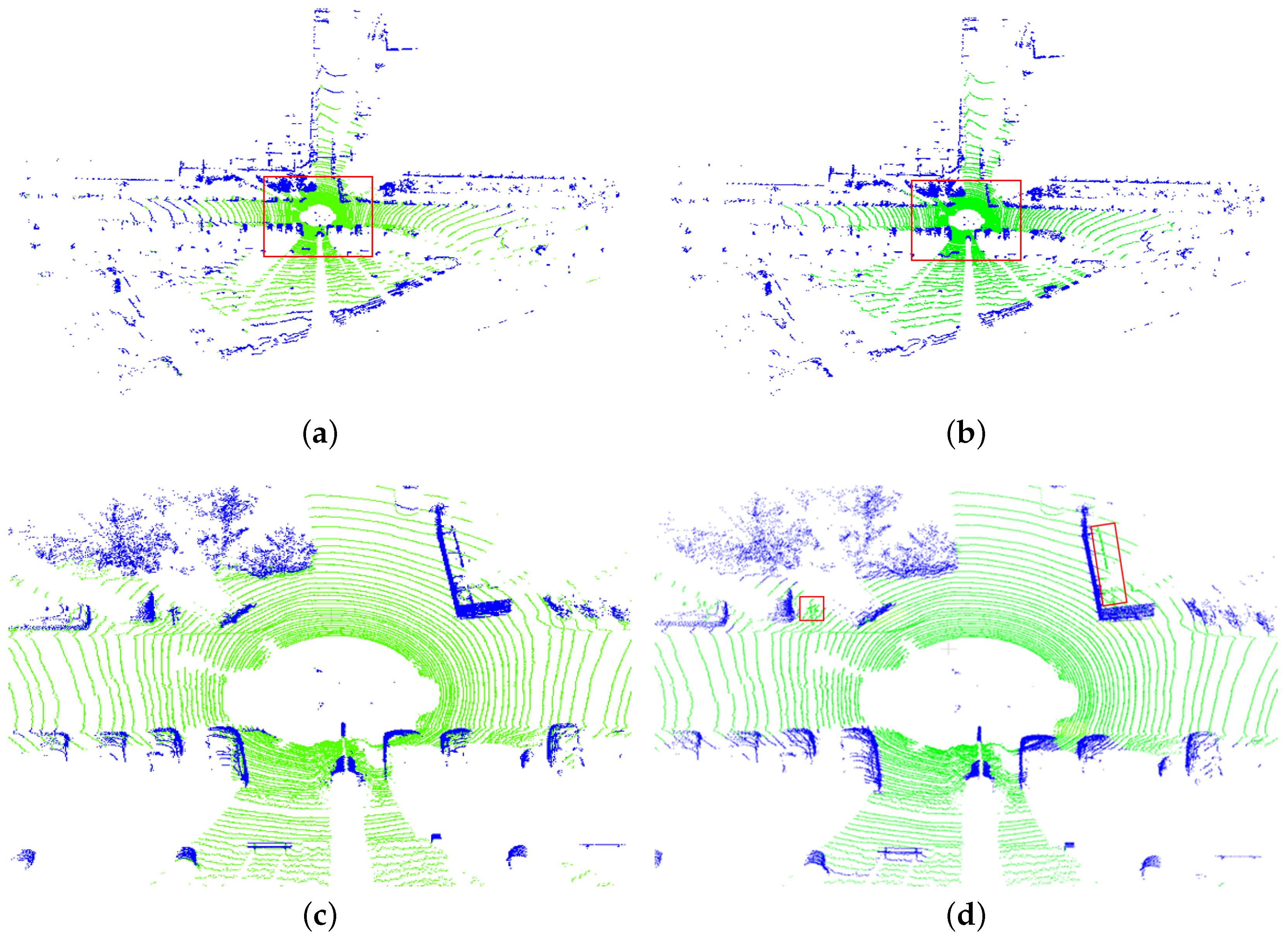
We select two point clouds in the KITTI data set. Both point clouds are road scenes with 110 k points. We manually label the point cloud. As shown in
Figure 5a, the green points are ground points, and the blue points are non-ground points. The red frame marked area in
Figure 5a is enlarged as shown in
Figure 5c.
The height of the ground of the first point cloud part is about −3 to 0.2 m. We set the fitting plane height parameter
to (−3, 0.2) and set the rejection threshold
to 1.5. After the parameter setting is completed, the point cloud is processed by the proposed method. The filtering result of the proposed method is shown in
Figure 5b. The red frame marked area in
Figure 5b is enlarged as shown in
Figure 5d. Comparing
Figure 5a,b, the method in this article can effectively distinguish ground points from other objects.
The results obtained by the proposed method are essentially consistent with the results of manual labeling. Comparing
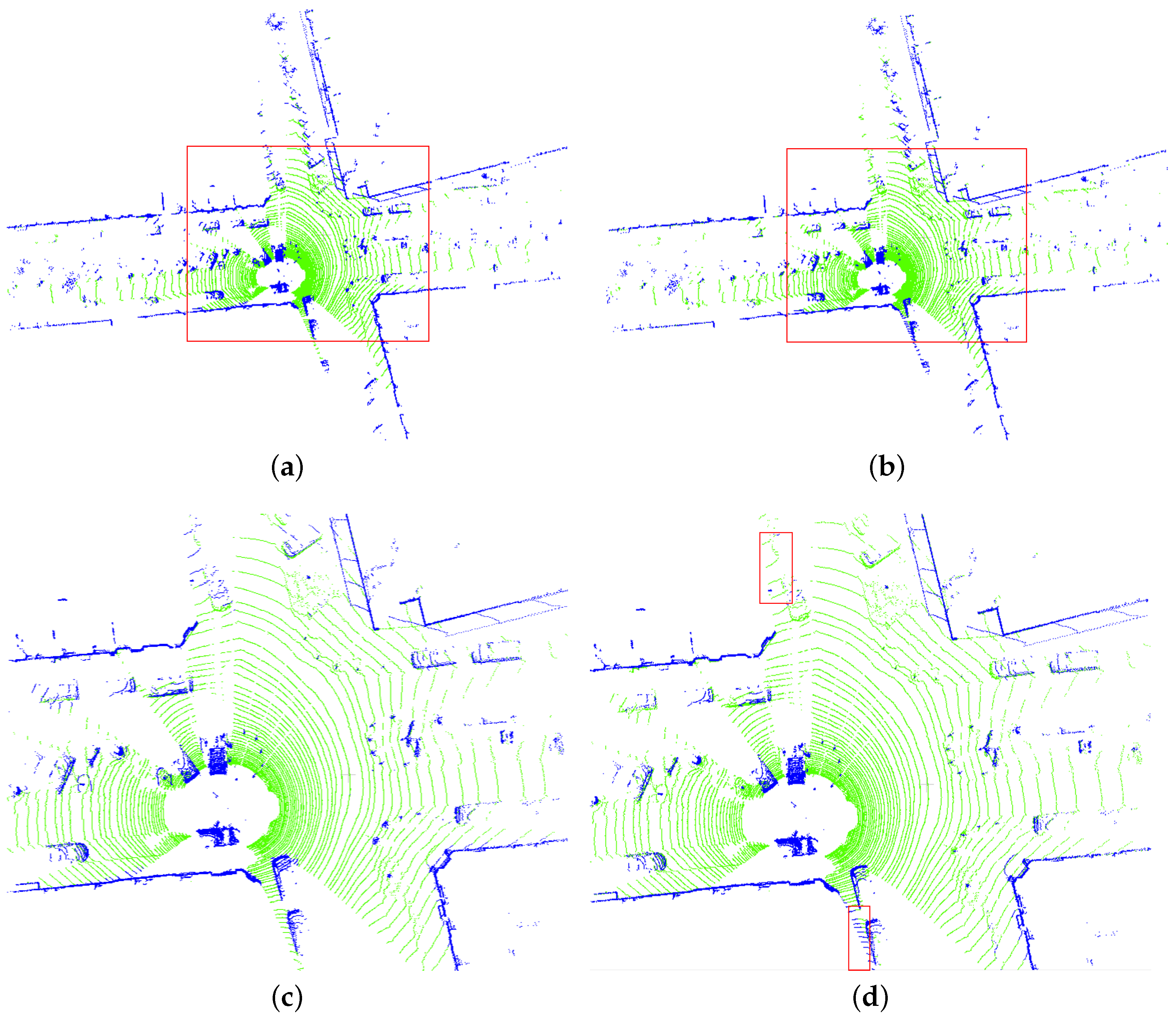
Figure 5c,d, the method in this article handles the details of the point cloud well, and can accurately distinguish ground points from non-ground points. A fact that can be demonstrated in
Figure 6 as in
Figure 5 is that the proposed method can better preserve details in the filtering results.
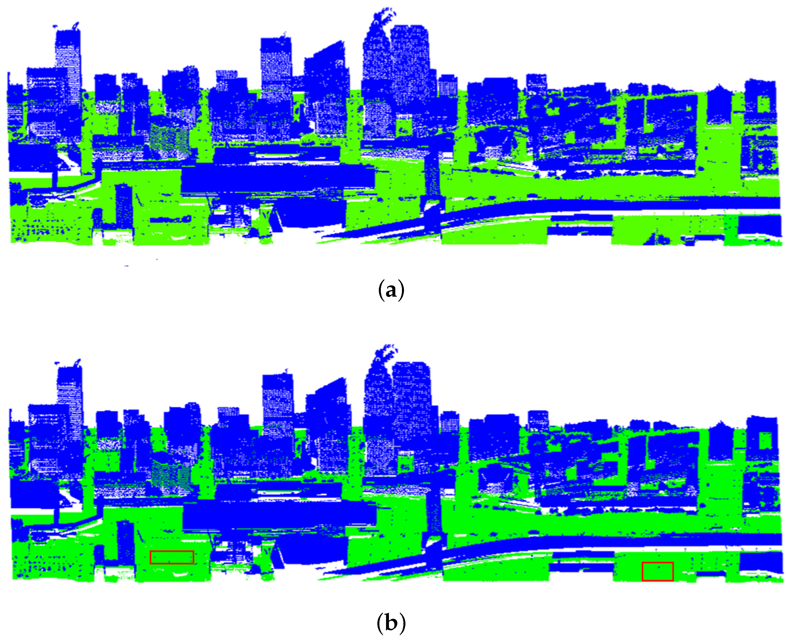
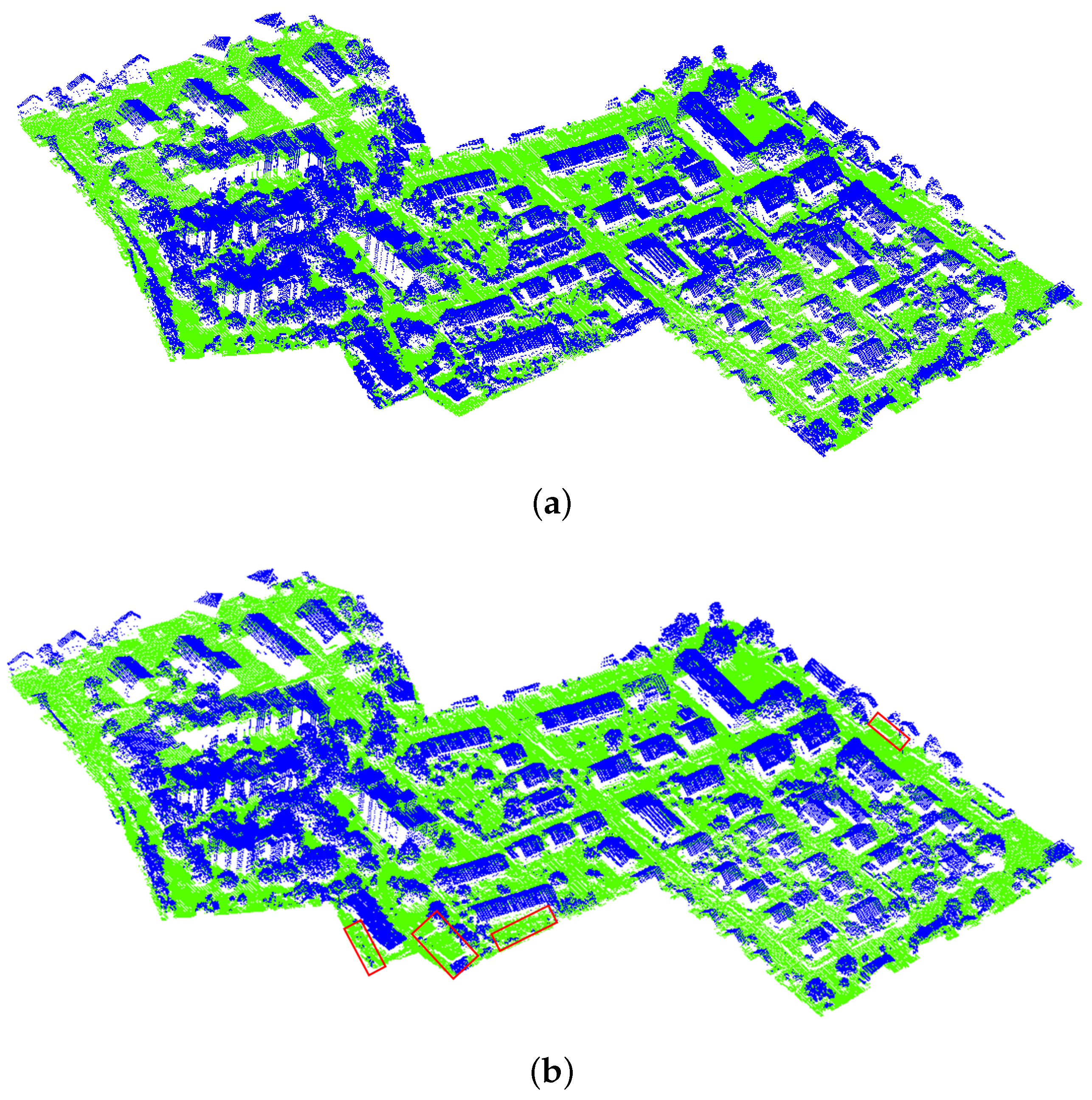
Toronto is an urban scene composed of 750 k points. The ground is relatively flat as shown in
Figure 7a. We set the fitting plane height parameter
to (40, 50) and set the rejection threshold
to 5. The result is shown in
Figure 7b. Comparing
Figure 7a,b, it can be seen that the method in this article can better distinguish large buildings from the ground. At the same time, it can take into account the details of the ground, and some small objects can be distinguished from the ground.
Vaihingen is a village scene with a total of 720 k points. The ground in this village is uneven as shown in
Figure 8a. We set the fitting plane height parameter
to (251, 270) and set the rejection threshold
to 15. The processing result of the proposed method is shown in
Figure 8b. It can be seen from the figure that the method in this article can adapt to complex scene of the point cloud with uneven ground.
4.2. Accuracy Comparison
The proposed method is compared with eight methods. Among these methods are recent and classic. Method I is the original RANSAC. Method II is progressive TIN densification [
47]. Method III is cloth simulation filter [
48]. Method IV is the multiscale curvature classification [
49]. Method V is active contours [
50]. Method VI is regularization method [
51]. Method VII is modified slope based filter [
52]. Method VIII is hierarchical modified block-minimum [
53]. The comparison of the first four methods is shown in
Table 1, and we show the different performance of each method applied to different data. The comparison of the last four methods is shown in
Table 2. We show the total error of filtering.
We use two data provided by ISPRS and two data in the KITTI dataset as experimental data. Error Type I, Error Type II, and the total error are used as evaluation indicators. The type I error represents the proportion of ground points erroneously assigned as nonground points, and the type II error represents the proportion of nonground points erroneously assigned as ground points. The total error is the proportion of all the point-cloud data that is misjudged and is used to evaluate the overall quality of the filtering results [
54].
As shown in
Table 1, compared with other methods, the error of the method in this article is relatively small. The mean value of the total errors of the proposed method is about 7.86%. The mean values of the total error of the remaining four methods are 18.4%, 9.57%, 8.5%, and 9.54%, respectively. Compared with Method I, the average error of the proposed method is reduced by about 10.54%. The comparison of the filtering results of these two methods is shown in
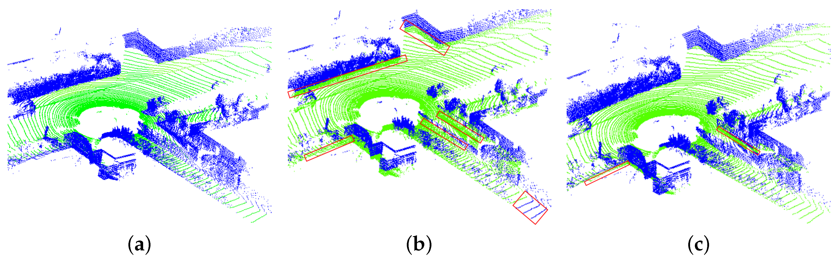
Figure 9. Compared with the current commonly used methods, the average error of the proposed method is reduced by at least 0.64%. The proposed method has a better comprehensive performance on the KITTI dataset and the datasets provided by ISPRS.
Compared with other methods, the proposed method can adapt to complex scenes and deal with the details in the point cloud. The advantage of this method is that it has high filtering accuracy on relatively flat ground. The comparison with the last four methods is shown in
Table 2. The average errors of other methods are significantly higher than those of the proposed method. This further confirms the high filtering accuracy of the proposed method.
4.3. 3D Object Detection Experiment and Efficiency Analysis
We explore the application of LiDAR ground filtering for 3D-object detection. We use the KITTI dataset. The vehicle is the detection object. We test three open-source 3D-object detection methods. Pretrained weights are used to detect objects in point clouds. The detection results of the unfiltered point cloud and the filtered point cloud are compared. The results are shown in
Table 3. It can be clearly seen that when the filtered point cloud is used for 3D-object detection in simple or moderate situations, the detection accuracy is significantly improved.
In the process of object detection, ground points are often interference information. After removing the ground points, each object is in an isolated state, and the object detection algorithm only needs to match the detected object from multiple isolated objects. This can reduce the difficulty of object detection, thereby, improving the performance of object detection. However, when it is used for difficult 3D-object detection, the detection accuracy is slightly reduced. The main reason is that the filtering takes away a small part of the point cloud at the object. The original identification is more difficult, and it is more difficult to detect if some information is missing.
The LiDAR ground filtering experiment was conducted on a computer with Intel Core i7 3.19-GHz CPU and 16-GB RAM. The calculation time of the proposed method is about 20 ms to process a point cloud of 100 k points. Current 3D-object detection algorithms generally run on platforms with high computing power. Furthermore, better computing platforms have strong parallel computing capabilities, and thus the time used for ground filtering can be further reduced.
We randomly select 20 point clouds in the KITTI dataset, manually annotate the ground and non-ground points, and record the number of ground and non-ground points. We found that the ground points account for about 40–60% of the entire point cloud. The computation time of the 3D-object detection method is related to the number of points in the point cloud. The lower the number of points in the point cloud, the lower the runtime. Therefore, the filtered point cloud can improve the speed of 3D-object detection. The times for the three object detection methods are shown in
Table 4. It can be clearly seen that the detection time is significantly reduced. The results show that the proposed method does not have a large impact on the time of the 3D-object detection method.
5. Conclusions
In this paper, we proposed an improved RANSAC LiDAR ground filtering method. We evaluated the proposed method using point clouds with different characteristics and compared the filtering accuracy with a variety of commonly used methods. The results show that the filtering accuracy of this method was improved by about 10% compared with the original method and by about 1% compared with the current advanced method. Furthermore, this method has higher filtering efficiency.
The proposed method is intended to be applied to 3D-object detection. Ground filtering can improve object detection accuracy under simple and moderate conditions on the KITTI dataset. Furthermore, this can reduce the time of object detection. When the proposed method is applied to 3D-object detection methods, the influence of the filtering time on object detection can be ignored. This paper demonstrates that ground filtering can be used as an auxiliary method to improve the accuracy of 3D-object detection. Therefore, the LiDAR ground filtering method deserves further in-depth study.
Author Contributions
Conceptualization, J.L. and B.W.; methodology, B.W.; software, J.G.; validation, B.W. and J.G.; formal analysis, J.L.; investigation, B.W.; resources, J.G.; data curation, J.G.; writing—original draft preparation, B.W.; writing—review and editing, J.L.; visualization, J.G.; supervision, J.L. All authors have read and agreed to the published version of the manuscript.
Funding
This research was funded by the 13th Five-Year Plan Funding of China, the Funding 41419029102 and the Funding 41419020107.
Data Availability Statement
ISPRS datasets was provided by the German Society for Photogram metry, Remote Sensing and Geoinformation (DGPF). KITTI datasets was provided by Karlsruhe Institute of Technology (KIT) and Toyota Technological Institute at Chicago (TTI-C).
Conflicts of Interest
The authors declare no conflict of interest.
References
- Niu, Z.; Xu, Z.; Sun, G. Design of a New Multispectral Waveform LiDAR Instrument to Monitor Vegetation. IEEE Geosci. Remote Sens. Lett. 2015, 12, 1506. [Google Scholar]
- Montealegre, A.L.; Lamelas, M.T.; Juan, D. A Comparison of Open-Source LiDAR Filtering Algorithms in a Mediterranean Forest Environment. IEEE J. Sel. Top. Appl. Earth Obs. Remote Sens. 2015, 8, 4072–4085. [Google Scholar] [CrossRef] [Green Version]
- Huang, S.Y.; Liu, L.M.; Dong, J. Review of ground filtering algorithms for vehicle LiDAR scans point-cloud data. Opto-Electron. Eng. 2020, 47, 190688-1–190688-12. [Google Scholar]
- Zhao, H.; Xi, X.; Wang, C. Ground Surface Recognition at Voxel Scale From Mobile Laser Scanning Data in Urban Environment. IEEE Geosci. Remote Sens. Lett. 2019, 99, 1–5. [Google Scholar] [CrossRef]
- You, H.; Li, S.; Xu, Y. Tree Extraction from Airborne Laser Scanning Data in Urban Areas. Remote Sens. 2021, 13, 3428. [Google Scholar] [CrossRef]
- Lecun, Y.; Bengio, Y.; Hinton, G. Deep learning. Nature 2015, 521, 436. [Google Scholar] [CrossRef] [PubMed]
- Zheng, W.; Tang, W.; Chen, S. CIA-SSD: Confident IoU-Aware Single-Stage Object Detector From Point Cloud. In Proceedings of the 35th AAAI Conference on Artificial Intelligence (AAAI), Online, 2–9 February 2021. [Google Scholar]
- Pang, S.; Morris, D.; Radha, H. CLOCs: Camera-LiDAR Object Candidates Fusion for 3D Object Detection. In Proceedings of the IEEE/RSJ International Conference on Intelligent Robots and Systems (IROS), Las Vegas, NV, USA, 25–29 October 2020. [Google Scholar]
- Li, Z.; Yao, Y.; Quan, Z.; Yang, W.; Xie, J. SIENet: Spatial Information Enhancement Network for 3D Object Detection from Point Cloud. In Proceedings of the IEEE Conference on Computer Vision and Pattern Recognition, Nashville, TN, USA, 20–25 June 2021. [Google Scholar]
- Zhou, Y.; Tuzel, O. VoxelNet: End-to-End Learning for Point Cloud Based 3D Object Detection. In Proceedings of the IEEE/CVF Conference on Computer Vision and Pattern Recognition (CVPR), Salt Lake City, UT, USA, 18–23 June 2018. [Google Scholar]
- Lang, A.H.; Vora, S.; Caesar, H. PointPillars: Fast Encoders for Object Detection From Point Clouds. In Proceedings of the IEEE/CVF Conference on Computer Vision and Pattern Recognition (CVPR), Long Beach, CA, USA, 15–20 June 2019. [Google Scholar]
- Shi, S.; Wang, X.; Li, H. PointRCNN: 3D Object Proposal Generation and Detection from Point Cloud. In Proceedings of the IEEE/CVF Conference on Computer Vision and Pattern Recognition (CVPR), Long Beach, CA, USA, 15–20 June2019. [Google Scholar]
- Zhou, D.; Fang, J.; Song, X. Joint 3D Instance Segmentation and Object Detection for Autonomous Driving. In Proceedings of the IEEE/CVF Conference on Computer Vision and Pattern Recognition (CVPR), Seattle, WA, USA, 13–19 June 2020. [Google Scholar]
- Miadlicki, K.; Pajor, M.; Sakow, M. Real-time ground filtration method for a loader crane environment monitoring system using sparse LIDAR data. In Proceedings of the IEEE International Conference on INnovations in Intelligent SysTems and Applications (INISTA), Gdynia, Poland, 3–5 July 2017. [Google Scholar]
- Fan, W.; Wen, C.; Tian, Y. Rapid Localization and Extraction of Street Light Poles in Mobile LiDAR Point Clouds: A Supervoxel-Based Approach. IEEE Trans. Intell. Transp. Syst. 2017, 18, 292. [Google Scholar]
- Golovinskiy, A.; Kim, V.G.; Funkhouser, T. Shape-based recognition of 3D point clouds in urban environments. In Proceedings of the IEEE International Conference on Computer Vision, San Francisco, CA, USA, 13–18 June 2010. [Google Scholar]
- Raguram, R.; Chum, O.; Pollefeys, M. USAC: A Universal Framework for Random Sample Consensus. IEEE Trans. Pattern Anal. Mach. Intell. 2013, 35, 2022–2038. [Google Scholar] [CrossRef]
- Ni, K.; Jin, H.G.; Dellaert, F. GroupSAC: Efficient Consensus in the Presence of Groupings. In Proceedings of the IEEE International Conference on Computer Vision, Kyoto, Japan, 27 September–4 October 2009. [Google Scholar]
- Nister, D. Preemptive RANSAC for Live Structure and Motion Estimation. In Proceedings of the IEEE International Conference on Computer Vision, Nice, France, 13–16 October 2003. [Google Scholar]
- Kilian, J.; Haala, N.; Englich, M. Capture and evaluation of airborne laser scanner data. Int. Arch. Photogramm. Remote Sens. 1996, 31, 383–388. [Google Scholar]
- Zhang, K.; Chen, S.C.; Whitman, D. A progressive morphological filter for removing nonground measurements from airborne LIDAR data. IEEE Trans. Geosci. Remote Sens. 2003, 41, 872–882. [Google Scholar] [CrossRef] [Green Version]
- Pirotti, F.; Guarnieri, A.; Vettore, A. Ground filtering and vegetation mapping using multi-return terrestrial laser scanning. ISPRS J. Photogramm. Remote Sens. 2013, 76, 56–63. [Google Scholar] [CrossRef]
- Trepekli, K.; Friborg, T. Deriving Aerodynamic Roughness Length at Ultra-High Resolution in Agricultural Areas Using UAV-Borne LiDAR. Remote Sens. 2013, 13, 3538. [Google Scholar] [CrossRef]
- Thrun, S.; Montemerlo, M.; Dahlkamp, H. Stanley: The Robot that Won the DARPA Grand Challenge. J. Field Robot. 2006, 23, 661–692. [Google Scholar] [CrossRef]
- Zhao, G.; Yuan, J. Curb detection and tracking using 3D-LIDAR scanner. In Proceedings of the IEEE International Conference on Image Processing, Melbourne, Australia, 15–18 September 2013. [Google Scholar]
- Douillard, B.; Underwood, J.; Kuntz, N. On the segmentation of 3D LIDAR point clouds. In Proceedings of the IEEE International Conference on Robotics & Automation, Shanghai, China, 9–13 May 2011. [Google Scholar]
- Kraus, K.; Pfeifer, N. Determination of terrain models in wooded areas with airborne laser scanner data. ISPRS J. Photogramm. Remote Sens. 1998, 53, 193–203. [Google Scholar] [CrossRef]
- Kobler, A.; Pfeifer, N.; Ogrinc, P. Repetitive interpolation: A robust algorithm for DTM generation from Aerial Laser Scanner Data in forested terrain. Remote Sens. Environ. 2007, 108, 9–23. [Google Scholar] [CrossRef]
- Qin, L.; Wu, W.; Tian, Y. LiDAR Filtering of Urban Areas with Region Growing Based on Moving-Window Weighted Iterative Least-Squares Fitting. IEEE Geosci. Remote Sens. Lett. 2017, 14, 841–845. [Google Scholar] [CrossRef]
- Gao, L.; Shi, W.; Zhu, Y. Novel Framework for 3D Road Extraction Based on Airborne LiDAR and High-Resolution Remote Sensing Imagery. Remote Sens. 2021, 13, 4766. [Google Scholar] [CrossRef]
- Fischler, M.A.; Bolles, R.C. Random Sample Consensus: A Paradigm for Model Fitting with Applications to Image Analysis and Automated Cartography. Commun. ACM 1981, 24, 381–395. [Google Scholar] [CrossRef]
- Myatt, D.R.; Torr, P.H.; Nasuto, S.J. NAPSAC: High Noise, High Dimensional Robust Estimation. In Proceedings of the British Machine Vision Conference, Cardiff, UK, 2–5 September 2002. [Google Scholar]
- Chum, O.; Matas, J. Matching with PROSAC—Progressive Sample Consensus. In Proceedings of the IEEE Conference on Computer Vision and Pattern Recognition, San Diego, CA, USA, 20–26 June 2005. [Google Scholar]
- Capel, D. An Effective Bail-Out Test for RANSAC Consensus Scoring. In Proceedings of the British Machine Vision Conference, Oxford, UK, 5–8 September 2005. [Google Scholar]
- Chum, O.; Matas, J. Optimal Randomized RANSAC. IEEE Trans. Pattern Anal. Mach. Intell. 2008, 30, 1472–1482. [Google Scholar] [CrossRef] [PubMed] [Green Version]
- Matas, J.; Chum, O. Randomized RANSAC with Sequential Probability Ratio Test. In Proceedings of the IEEE International Conference on Computer Vision, Beijing, China, 17–21 October 2005. [Google Scholar]
- Chum, O.; Matas, J.; Kittler, J. Locally Optimized RANSAC. In Proceedings of the DAGM-Symposium Pattern Recognition, Magdeburg, Germany, 10–12 September 2003. [Google Scholar]
- Raguram, R.; Frahm, J.; Pollefeys, M. Exploiting Uncertainty in Random Sample Consensus. In Proceedings of the IEEE International Conference on Computer Vision, Kyoto, Japan, 27 September–4 October 2009. [Google Scholar]
- Yang, Z.; Sun, Y.; Liu, S.; Shen, X.; Jia, J. STD: Sparse-to-dense 3D object detector for point cloud. In Proceedings of the IEEE International Conference on Computer Vision, Kyoto, Japan, 27 September–4 October 2019. [Google Scholar]
- Liu, Z.; Zhou, S.; Suo, C. LPD-Net: 3D point cloud learning for large-scale place recognition and environment analysis. In Proceedings of the IEEE International Conference on Computer Vision, Kyoto, Japan, 27 September–4 October 2019. [Google Scholar]
- Zhang, W.; Xiao, C. PCAN: 3D attention map learning using contextual information for point cloud based retrieval. In Proceedings of the IEEE/CVF Conference on Computer Vision and Pattern Recognition (CVPR), Long Beach, CA, USA, 15–20 June 2019. [Google Scholar]
- Paigwar, A.; Erkent, O.; Wolf, C. Attentional PointNet for 3D-object detection in point clouds. In Proceedings of the IEEE/CVF Conference on Computer Vision and Pattern Recognition (CVPR), Long Beach, CA, USA, 15–20 June 2019. [Google Scholar]
- Shi, S.; Guo, C.; Jiang, L. PV-RCNN: Point-voxel feature set abstraction for 3D-object detection. In Proceedings of the IEEE/CVF Conference on Computer Vision and Pattern Recognition (CVPR), Seattle, WA, USA, 13–19 June 2020. [Google Scholar]
- Aiswarya, G.; Valsaraj, N.; Vaishak, M. Content-based 3D image retrieval using point cloud library a novel approach for the retrieval of 3D images. In Proceedings of the International Conference on Communication and Signal Processing, Melmaruvathur, India, 6–8 April 2017. [Google Scholar]
- Sithole, G.; Vosselman, G. Comparison of filtering algorithms. Int. Arch. Photogramm. Remote Sens. 2003, 34, 1–8. [Google Scholar]
- Wang, B.; Frémont, V.; Rodríguez, S.A. Color-based road detection and its evaluation on the KITTI road benchmark. In Proceedings of the IEEE Intelligent Vehicles Symposium Proceedings, Dearborn, MI, USA, 8–11 June 2014. [Google Scholar]
- Zhang, J.; Lin, X. Filtering airborne LiDAR data by embedding smoothness-constrained segmentation in progressive TIN densification. ISPRS J. Photogramm. Remote Sens. 2013, 81, 44–59. [Google Scholar] [CrossRef]
- Zhang, W.; Qi, J.; Wan, P. An Easy-to-Use Airborne LiDAR Data Filtering Method Based on Cloth Simulation. Remote Sens. 2016, 8, 501. [Google Scholar] [CrossRef]
- Evans, J.S.; THudak, A. A multiscale curvature algorithm for classifying discrete return LiDAR in forested environments. IEEE Trans. Geosci. Remote Sens. 2007, 45, 1029–1038. [Google Scholar] [CrossRef]
- Elmqvist, M.; Jungert, E.; Lantz, F.; Persson, A.; Soderman, U. Terrain modelling and analysis using laser scanner data. Int. Arch. Photogramm. Remote Sens. 2001, 34, 219–227. [Google Scholar]
- Sohn, G.; Dowman, I. Terrain Surface Reconstruction by the Use Of Tetrahedron Model With the MDL Criterion. Int. Arch. Photogramm. Remote Sens. 2002, 34, 336–344. [Google Scholar]
- Roggero, M. Airborne Laser Scanning: Clustering in raw data. Int. Arch. Photogramm. Remote Sens. 2001, 34, 227–232. [Google Scholar]
- Wack, R.; Wimmer, A. Digital Terrain Models From Airborne Laser Scanner Data—A Grid Based Approach. Int. Arch. Photogramm. Remote Sens. 2002, 34, 293–296. [Google Scholar]
- Sithole, G.; Vosselman, G. Report: ISPRS Comparison of Filters. Available online: http://www.itc.nl/isprswgIII-3/filtertest/ (accessed on 27 December 2016).
Figure 1.
Flowchart of Universal-RANSAC.
Figure 1.
Flowchart of Universal-RANSAC.
Figure 2.
Flowchart of the proposed method.
Figure 2.
Flowchart of the proposed method.
Figure 3.
Schematic diagram of a point cloud grouping. According to the height, the point cloud is divided into two groups, the blue group and the green group. It is clear that the green group contains more inliers.
Figure 3.
Schematic diagram of a point cloud grouping. According to the height, the point cloud is divided into two groups, the blue group and the green group. It is clear that the green group contains more inliers.
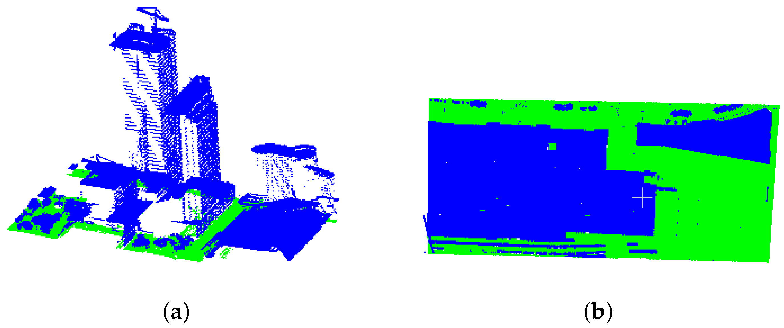
Figure 4.
Special cases. The green points are ground points, and the blue points are non-ground points. (a) The number of points on the side of the building is greater than the points on the ground. (b) The number of points on the top of the building is greater than the points on the ground.
Figure 4.
Special cases. The green points are ground points, and the blue points are non-ground points. (a) The number of points on the side of the building is greater than the points on the ground. (b) The number of points on the top of the building is greater than the points on the ground.
Figure 5.
The result of the proposed method. The red box area in (d) is classified incorrectly. (a) The point cloud manually labeled. (b) The point cloud processed by the proposed method. (c) The red box area in (a). (d) The red box area in (b).
Figure 5.
The result of the proposed method. The red box area in (d) is classified incorrectly. (a) The point cloud manually labeled. (b) The point cloud processed by the proposed method. (c) The red box area in (a). (d) The red box area in (b).
Figure 6.
The result of the proposed method. The red box area in (d) is classified incorrectly. (a) The point cloud manually labeled. (b) The point cloud processed by the proposed method. (c) The red box area in (a). (d) The red box area in (b).
Figure 6.
The result of the proposed method. The red box area in (d) is classified incorrectly. (a) The point cloud manually labeled. (b) The point cloud processed by the proposed method. (c) The red box area in (a). (d) The red box area in (b).
Figure 7.
The result of the proposed method. (a) The point cloud manually labeled. (b) The point cloud processed by the proposed method. The red box area in (b) is classified incorrectly.
Figure 7.
The result of the proposed method. (a) The point cloud manually labeled. (b) The point cloud processed by the proposed method. The red box area in (b) is classified incorrectly.
Figure 8.
The result of the proposed method. (a) The point cloud manually labeled. (b) The point cloud processed by the proposed method. The red box area in (b) is classified incorrectly.
Figure 8.
The result of the proposed method. (a) The point cloud manually labeled. (b) The point cloud processed by the proposed method. The red box area in (b) is classified incorrectly.
Figure 9.
The results of the comparison between the method proposed in this article and the RANSAC plane fitting method. Green points are the ground points, blue points are the non-ground points. The red boxes in (b,c) are classified incorrectly. (a) The point cloud manually labeled. (b) The point cloud processed by the RANSAC. (c) The point cloud processed by the method proposed in this article.
Table 1.
Comparison of the errors of the proposed method and other methods.
Table 1.
Comparison of the errors of the proposed method and other methods.
| Method | Data | Type I Error (%) | Type II Error (%) | Total Error (%) |
|---|
| Proposed Method | Toronto | 8.11 | 2.52 | 5.41 |
| Vaihingen | 2.38 | 17.74 | 9.28 |
| KITTI1 | 0.94 | 10.15 | 6.25 |
| KITTI2 | 5.67 | 15.97 | 10.50 |
| Method I | Toronto | 10.59 | 25.62 | 18.45 |
| Vaihingen | 24.65 | 19.75 | 22.53 |
| KITTI1 | 18.64 | 12.65 | 15.86 |
| KITTI2 | 16.47 | 17.57 | 16.75 |
| Method II | Toronto | 8.45 | 6.87 | 7.86 |
| Vaihingen | 13.58 | 11.96 | 12.77 |
| KITTI1 | 3.42 | 12.21 | 7.96 |
| KITTI2 | 7.65 | 11.14 | 9.71 |
| Method III | Toronto | 14.56 | 4.78 | 9.27 |
| Vaihingen | 10.64 | 6.98 | 8.40 |
| KITTI1 | 1.48 | 8.48 | 4.71 |
| KITTI2 | 14.68 | 8.57 | 11.67 |
| Method IV | Toronto | 12.54 | 6.86 | 8.74 |
| Vaihingen | 5.76 | 17.86 | 11.46 |
| KITTI1 | 3.86 | 11.53 | 7.34 |
| KITTI2 | 13.75 | 8.64 | 10.65 |
Table 2.
Comparison of the total errors of the proposed method and other methods.
Table 2.
Comparison of the total errors of the proposed method and other methods.
| Data | Method V (%) | Method VI (%) | Method VII (%) | Method VIII (%) | Proposed (%) |
|---|
| Toronto | 12.43 | 8.54 | 15.64 | 6.08 | 5.41 |
| Vaihingen | 9.06 | 11.53 | 14.53 | 11.46 | 9.28 |
| KITTI1 | 7.75 | 9.68 | 16.34 | 5.75 | 6.25 |
| KITTI2 | 14.64 | 15.57 | 11.91 | 16.45 | 10.50 |
| average | 10.97 | 11.33 | 14.61 | 9.94 | 7.86 |
Table 3.
Comparison of accuracy before and after ground filtering.
Table 3.
Comparison of accuracy before and after ground filtering.
| | | Raw Point Cloud (%) | No Ground Point Cloud (%) |
|---|
| CIA-SSD | Easy | 89.59 | 90.57 |
| Mod | 80.28 | 82.04 |
| Hard | 72.87 | 74.46 |
| CLOCs | Easy | 89.16 | 90.34 |
| Mod | 82.28 | 83.64 |
| Hard | 77.23 | 75.85 |
| SIENet | Easy | 88.22 | 90.47 |
| Mod | 81.71 | 85.15 |
| Hard | 77.22 | 73.74 |
Table 4.
Comparison of efficiency before and after ground filtering.
Table 4.
Comparison of efficiency before and after ground filtering.
| | Raw Point Cloud (ms) | No Ground Point Cloud (ms) |
|---|
| CIA-SSD | 30 | 22 |
| CLOCs | 100 | 70 |
| SIENet | 80 | 55 |
| Publisher’s Note: MDPI stays neutral with regard to jurisdictional claims in published maps and institutional affiliations. |
© 2022 by the authors. Licensee MDPI, Basel, Switzerland. This article is an open access article distributed under the terms and conditions of the Creative Commons Attribution (CC BY) license (https://creativecommons.org/licenses/by/4.0/).


