Tracking a Rain-Induced Low-Salinity Pool in the South China Sea Using Satellite and Quasi-Lagrangian Field Observations

Abstract

A low-salinity pool (LSP) was observed in the northeastern South China Sea on 8–10 August 2018. Employing satellite and field observations, as well as widely used HYbrid Coordinate Ocean Model (HYCOM) Analysis data, we investigated the distribution, origin and evolution of the LSP. A bowl-like structure of the LSP was observed from field observations and is also indicated by the HYCOM Analysis data. Spatially, the LSP extended 20 m deep vertically and spread at least 45 km laterally. Particle tracking simulations using satellite-observed precipitation and surface currents revealed the origin and evolution of the LSP. It is found that the LSP was induced by a heavy rainfall event two days prior to the field observations, evidenced by the significant correlation between the rainfall and salinity anomaly. The vertical expansion of the LSP was favored by nocturnal convection, but was restricted by the strong stratification at its base, which appeared to have prohibited development of convective instabilities as indicated by the observed vertical variation of the turbulent dissipation rate. The formation of a barrier layer due to the LSP restricted vertical heat exchanges, and as a result a thin temperature inversion layer was formed as the surface temperature dropped due to the nighttime cooling and mixing with the cold rainwater. The thermohaline structure favored development of diffusive convection, which is evidenced by the observation that the diapycnal diffusivity for heat (K_T) was one order of magnitude larger than that for density (K_ρ). Overall, this study provides novel insights into how the upper ocean responds to rainfall with satellite and field observations.

1. Introduction

Near-surface freshening due to rainfall modifies density distribution of the upper ocean and may generate a rain-induced low-salinity pool (LSP, also referred to as “low-salinity patches”, “freshwater plumes” or “freshwater lenses”, associated with a strong rainfall event(s)), which affects mixed layer dynamics and air–sea exchanges as well as climate [1,2]. In tropical open oceans, freshwater lenses are formed by frequent and intense precipitations, which inject a large amount of fresh rainwater into the upper ocean and eventually get dispersed due to vertical and lateral mixing processes. In most cases, a rain-induced salinity anomaly has a spatial scale of O(10) km horizontally and O(1–10) m vertically and lasts for O(1–10) h. The scale is affected by the amount of precipitation, drift due to wind and ambient currents and the characteristics of mixing [2,3,4,5].

The rain-induced LSP plays an important role in modulating the stratification of the upper ocean. The formation and evolution of an LSP results in strong vertical stratification at its base, which can suppress turbulent exchange with the deeper water. It can form a low-density layer and enhance surface currents [6,7], analogous to the warm diurnal layer formed by daytime solar heating [8]. This freshwater flux-induced stratification is an important factor for the formation of a barrier layer, which is defined as a layer between the isopycnic (isohaline) layer and the isothermal layer when the latter is deeper [9,10,11]. A temperature inversion (temperature increases with depth) usually occurs when a cold and freshwater cap exists at the surface [12,13,14], and this combination of unstable thermal stratification and stable haline stratification is conducive to the development of diffusive convection (a type of double diffusion). Recently, Walesby et al. reported observations of rain-induced double diffusion based on microstructure profiling measurements in the near-surface layer [15].

In addition to the aforementioned impacts on vertical structures and processes, rainfall events can also produce localized freshwater plumes, which tend to spread laterally as intrusions. A series of observations and numerical simulations were performed by Soloviev et al. [16,17,18], and it was found that wind stress interacting with near-surface freshwater lenses can lead to an asymmetry relative to the wind direction (sharper frontal interfaces and enhanced mixing on the upwind side). The drift induced by the wind and ambient currents can expand the low salinity water to a spatial scale far larger than the size of the original rainfall patch, and it may induce a fresh bias in satellite measurements of the sea surface salinity (SSS) [18,19,20,21], especially in typical rainy regions such as the inter-tropical convergence zone, Indo-Pacific warm pool and monsoon-forced area. Moreover, rainfall can modulate surface gravity waves and enhance near-surface currents at the expense of wave growth [22].

Rainfall can also influence biogeochemical processes in the upper ocean, such as phytoplankton productivity and air–water gas exchange. Heavy rainfall caused by tropical cyclones can cause phytoplankton blooming [23]. At a longer time scale, marine phytoplankton in tropical oceans appears to benefit from the increasing rainfall to avoid dramatic declines in productivity by local warming [24]. The enhancement of air–water gas exchange by rainfall was studied with laboratory experiments [25,26] and model ocean experiments (at the artificial ocean at Biosphere 2) [27,28]. It is found that the enhancement is caused by an enhanced gas transport rate at the air–water interface and surface layer chemical dilution.

The South China Sea (SCS) is a large tropical marginal sea affected by the East-Asian monsoon. The prevailing winds are northeasterly in winter and southwesterly in summer [29]. Southwest trade winds often bring heavy rainfall, especially in the eastern SCS [30,31]. It has been noted that these rainfalls contribute to the formation of the barrier layer [32] and seasonal variations of the near-surface salinity [31,33]. However, direct observations of how the upper ocean responds to rainfall remain very sparse, especially in the SCS. One major reason is that rain-induced fresher water is usually sparsely distributed and gets dispersed quickly in the upper ocean, making it very difficult to predict, capture and observe in field observations.

In this study, we report on a rain-induced LSP observed during a field campaign in the northeastern SCS. The LSP was tracked as we conducted quasi-Lagrangian field observations during cruising along the looping path of the Kuroshio intrusion into the SCS. By integrating cruise-based field measurements, satellite observations and HYCOM data, we investigate the formation, evolution and impact of the LSP. This paper is organized as follows: Section 2 describes the field measurements, satellite and HYCOM Analysis data used in this study and introduces particle tracking simulations used to reveal the horizontal evolution of LSP. In Section 3, we investigate the formation and evolution of the LSP, focusing on both horizontal and vertical processes. The characteristics and generation mechanisms of the inversion layer, as well as its effects on diapycnal mixing, are also described. We summarize the results and draw conclusions in Section 4.

2. Data and Method

The field observations were carried out onboard the R/V TAN KAH KEE (TKK) in the northeastern SCS, west of the Luzon Strait, from 09:00 on 8 August to 06:30 on 10 August, in 2018 (local time). The R/V track was roughly along the looping path of the Kuroshio intrusion to the SCS, which was accompanied by an anticyclonic eddy, as clearly indicated by the spatial pattern of absolute dynamic topography (Figure 1). Hydrological, microstructure and meteorological data were collected during the 46-h observation period (along a 128 km-long R/V track). For revealing the formation and evolution of the LSP, satellite and HYCOM Analysis data were also used to complement the field observations.

2.1. Field Observations and Data Processing

Twenty-three vertical turbulence profiles were collected using a free-fall microstructure profiler (VMP-500, Rockland Scientific Ltd., Victoria, BC, Canada). The processing of the microstructure data followed the recommendations of Roget et al. [34] using instrument and probe specifics provided by the manufacturer. The turbulent kinetic energy (TKE) dissipation rate (ε) was calculated by fitting the Nasmyth spectrum to the measured shear spectra over consecutive 3 s segments with a 50% overlap. As a result, vertical profiles of ε were obtained with a vertical spacing of ~2 m. The dissipation of thermal variance (χ) was calculated by integrating the resolved temperature spectrum or fitting its inertial-convective subrange, depending on whether inertial-convective subrange is well resolved (for details see ref. [35]). The diapycnal diffusivity of density (K_ρ) was estimated using the Osborn [36] formula:

$$K_{\rho }=\Gamma \frac{\epsilon }{N^2}.$$

(1)

where the mixing efficiency Γ was taken as a canonical value 0.2 [37] and N is the background buoyancy frequency. The diapycnal diffusivity of heat (K_T) was estimated following the Osborn and Cox [38] relation:

$$K_T=\frac{0.5\chi }{{\left(\frac{\partial \overline{T}}{\partial z}\right)}^2}.$$

(2)

where $\overline{T}$ is the background temperature. Besides two shear probes and two FP07 fast-response thermistors, the VMP was also equipped with an ancillary SBE-3 thermistor.

Nineteen regular hydrographic profiles were collected with a conductivity–temperature–depth (CTD) system (SBE 911plus). The data were processed through the SBE standard quality control procedure and eventually averaged into 0.1 m bins.

In addition, underway data were also obtained. Horizontal velocities were recorded using a shipboard acoustic Doppler current profiler (SADCP, 300 kHz). The SADCP continuously collected velocity profiles (averaged into 2 min bins) in 45 bins of 2 m thick below ~10 m. The surface temperature (SST) and salinity (SSS) data were collected using a thermosalinograph SBE-21 at ~5 m depth every 10 s (averaged to every 1 min). Wind speed, wind direction, surface air temperature, precipitation, relative humidity and solar radiation were recorded every minute during the observations from the R/V’s Automatic Weather Station (AWS).

The Turner angle is calculated as:

$$\mathrm{Tu}={\tan }^{-1}\left[\alpha (\partial \overline{T}/\partial z)+\beta (\partial \overline{S}/\partial z),\alpha (\partial \overline{T}/\partial z)-\beta (\partial \overline{S}/\partial z)\right],$$

(3)

where α and β are coefficients of thermal expansion and haline contraction, respectively.

The shear squared is calculated as

$$S^2={\left(\frac{\partial u}{\partial z}\right)}^2+{\left(\frac{\partial v}{\partial z}\right)}^2,$$

(4)

where u and v are the zonal and meridional velocity components, respectively.

The squared buoyancy frequency is calculated as

$$N^2=-\frac{g}{{\rho }_0}\frac{\partial \rho }{\partial z},$$

(5)

where g is the acceleration due to gravity, ρ is potential density and ρ₀ is a reference density (1020 kg m⁻³).

2.2. Satellite Observations and Particle Tracking Simulations

We used a set of satellite observations to show the observation background and the horizontal processes of the evolution of the LSP. The satellite altimeter data from AVISO have a horizontal resolution of 0.25° for the daily absolute dynamic topography and surface geostrophic velocities. The half-hourly level 3 precipitation data from Global Precipitation Measurement (GPM, IMERG Final Run) have a horizontal resolution of 0.1° [39]. The hourly gridded ocean surface current data used in particle tracking simulations have a horizontal resolution of 0.25°. The data were produced by combining the altimeter-derived surface geostrophic velocities and modeled Ekman currents using ECMWF ERA-Interim wind stress data [40].

In order to study the origin and distribution of the LSP, we conducted particle tracking simulations (PTS) based on satellite-observed precipitation and sea surface velocity combining altimeter-derived surface geostrophic velocities and modeled Ekman currents. We used the Python package “Parcels” from the OceanParcels project [41,42], which simulates the particles’ trajectories using a fourth-order Runge-Kutta scheme. Regarded as passive particles, rainwater can be advected by surface currents without considering vertical mixing or horizontal diffusion. Treated as a moving rain gauge, a passive particle can hold the rainwater and then drift together. Therefore, the rainwater can not only be accumulated but also be advected as

$$R_{PTS}={\displaystyle \sum _{i=0}^n\left[Rai{n}_i\left(x_i,y_i,t_i\right)\times \Delta t\right]},$$

(6)

where R_PTS is the accumulated rainwater indicated by the particle, (x_i, y_i) is the position of the particle, Rain_i is the rain rate at time t = t_i, Δt is time stepping and t_i = i × Δt. Then the results are interpolated at uniform grid points. To compare the results from PTS and field observations, R_PTS is interpolated to the R/V track as the rainwater “measured” by shipboard (R_PTS·ship). In this study, the particles were released at 9:00 on 7 August and then freely moved with time at a step of 30 min. Correspondingly, its accumulation was calculated and regarded as the rainwater in the analysis.

Although convection and mixing cannot be ignored in the real ocean, our idealized simulations provide a qualitative analysis of how the LSP forms, especially on a short time scale. Treating the R/V as a rain gauge (supporting the rainfall from GPM accumulated as the R/V drifted), we can get local accumulated rainwater R_local without considering the horizontal advection (under the background currents) of rainwater. Descriptions of three accumulated rainwater values are shown in

Table 1. Descriptions of three accumulated rainwater values.

Values	Descriptions
RPTS	Gridded data of time integration of the rain rate along particles’ tracks
RPTS·ship	RPTS along the R/V track
Rlocal	Time integration of the rain rate along the R/V track

. The results of PTS are analyzed in Section 3.2.

2.3. Supporting Data

The HYCOM Analysis data were used in this study to provide additional information. This includes three-dimensional hydrographic and their temporal variations, which were limited in the field and satellite observations.

The HYCOM Global Ocean Forecasting System (GOFS) 3.1 data at a horizontal resolution of 0.08° (about 8–9 km in the study region) and a temporal resolution of 3 h with 41 vertical layers were used in this study. The salinity and sea surface height data were the key parameters used in our analysis.

3. Results and Discussions

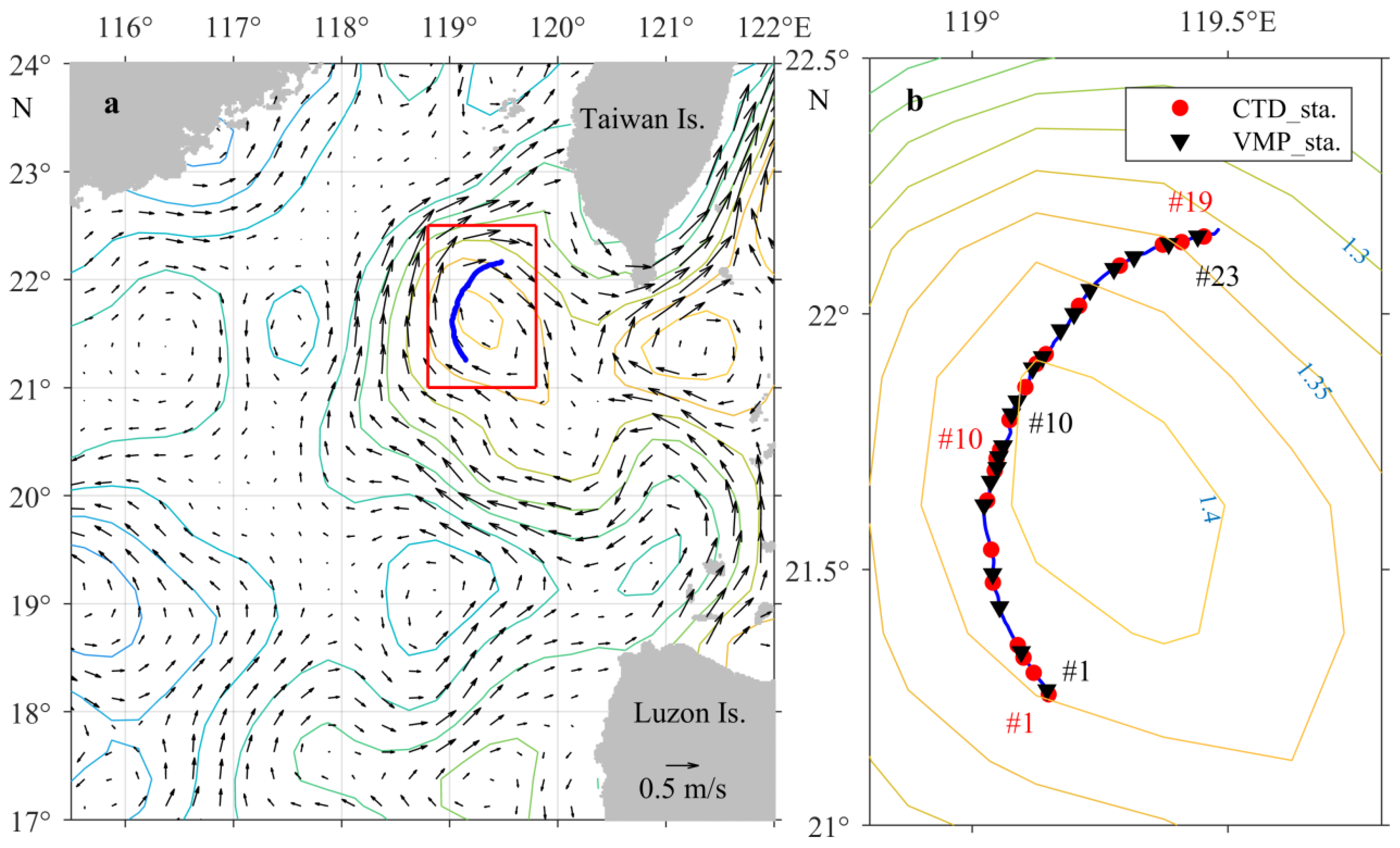
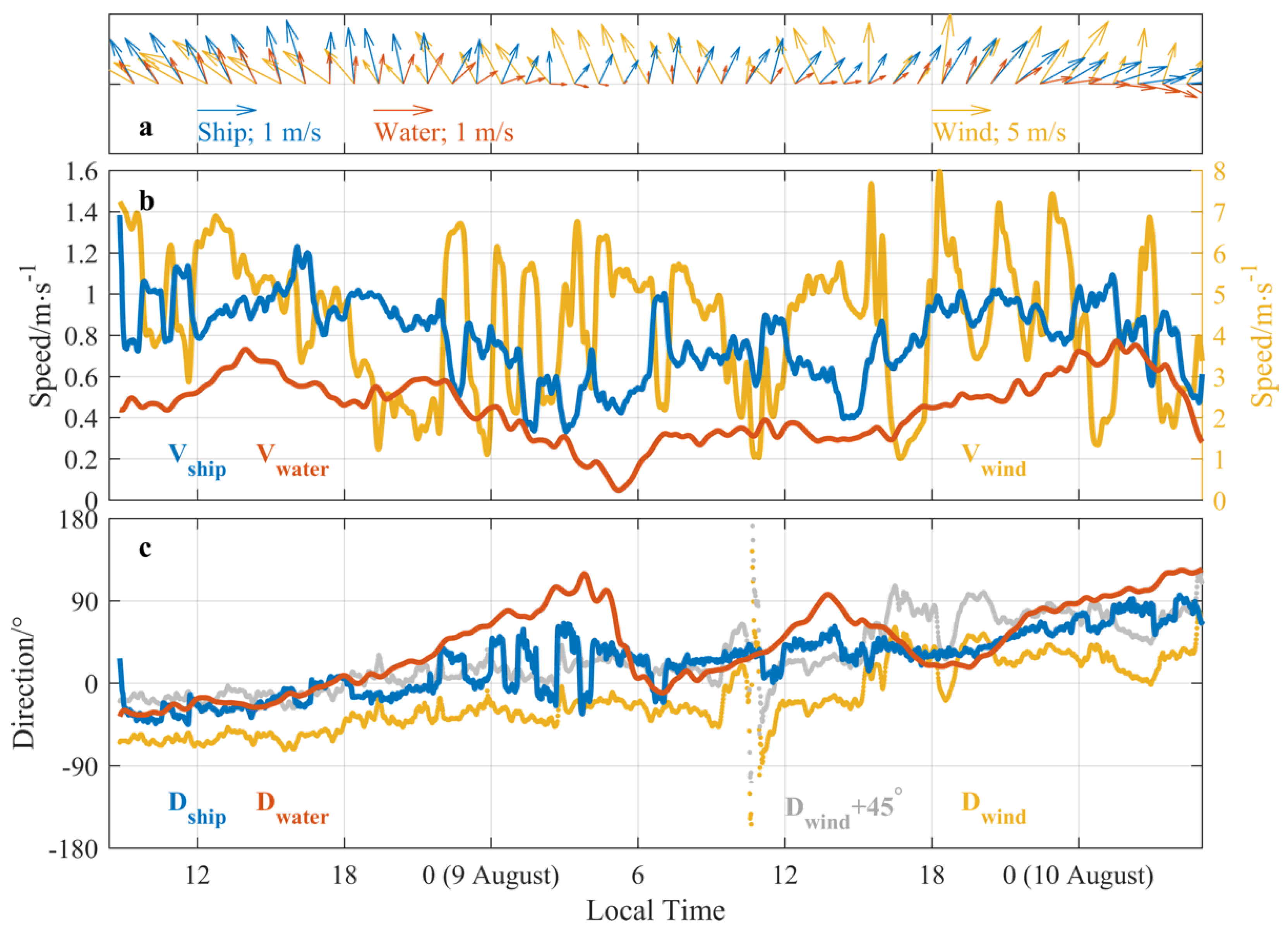
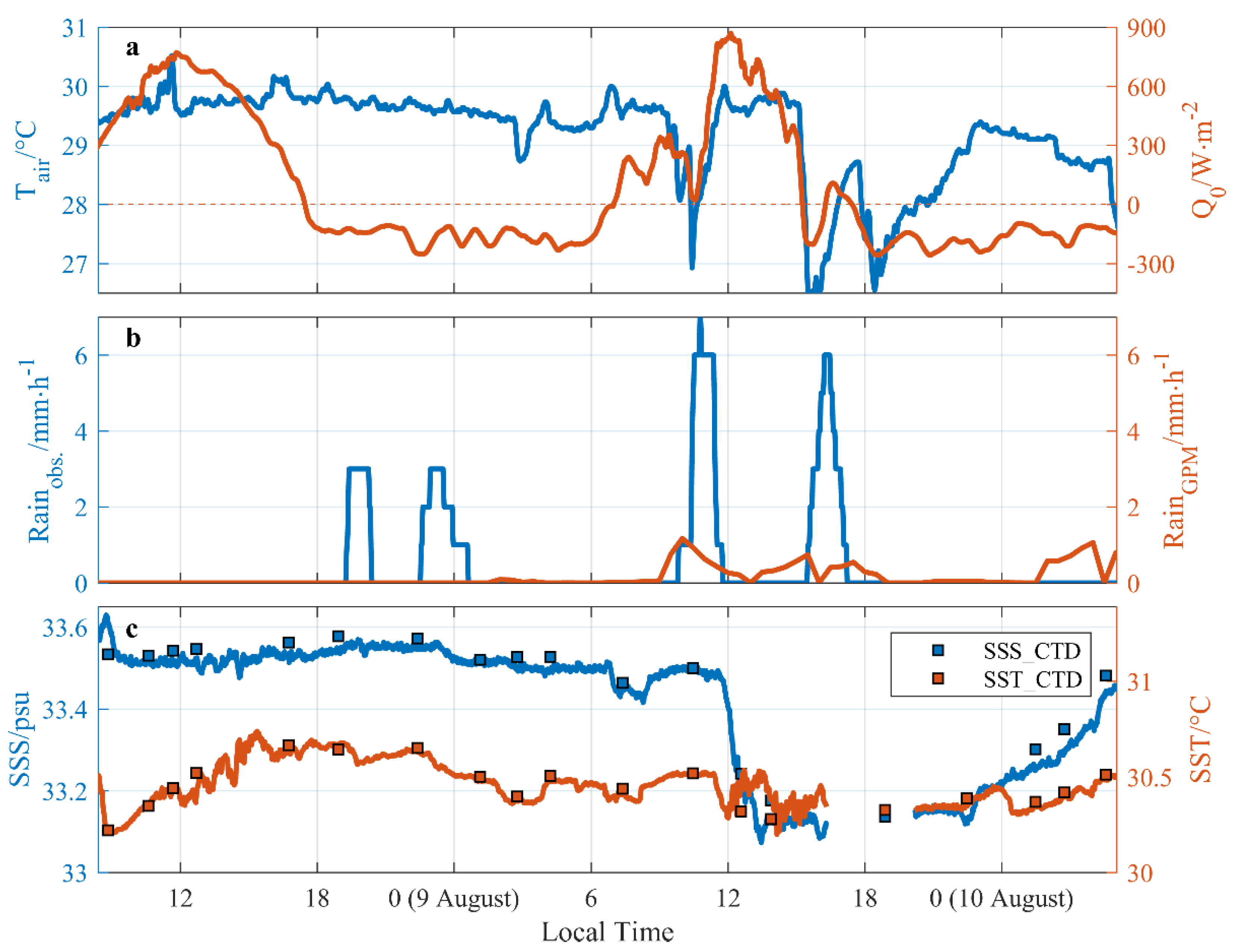
3.1. Environmental Context

During the field campaign along the looping path of the Kuroshio intrusion, we carried out quasi-Lagrangian observations, i.e., the R/V drifted without engine power. As shown in Figure 1, the trajectory of the R/V was roughly along a strong geostrophic current.

The trajectory was affected by both the sea surface current and the wind. As shown in Figure 2, the R/V drift speed (V_ship) was well correlated with the surface current speed (V_water), but the former is almost twice as high as that of the latter (mean speeds were 0.78 m/s and 0.44 m/s, respectively). V_water was relatively small (0.1–0.3 m/s) near the anticyclonic eddy center but large (0.4–0.7 m/s) near its edge in the early and late stages. The wind speed (V_wind) varied from 1 to 8 m/s during the observation period, and the mean wind speed was 4.2 m/s. The direction of the R/V drift velocity (D_ship) and the wind velocity (D_wind) both changed from the northwest to the northeast, but the former was about 45° larger than the latter. Moreover, the direction of the surface current velocity (D_water) was also close to D_ship except for the position near the anticyclonic eddy core at the middle of the R/V track. To investigate the relationship among the drifting velocity of the R/V, the surface current and the wind velocity, we fitted the observation data to the following formula:

$${\overrightarrow{V}}_{ship}={\lambda }_1{\overrightarrow{V}}_{water}+{\lambda }_2{\overrightarrow{V}}_{wind},$$

(7)

and obtained λ₁ = 1.293 and λ₂ = 0.056 through best fitting. We can quantify the contributions of the surface current and the wind by comparing the two terms on the right-hand side of Equation (7). It is found that the surface current contributed 71% of the drifting while the wind contributed 29%.

In summary, we put forward a toy model, i.e., Equation (7), for estimating the R/V track and quantifying the contributions of the surface current and wind to the drift of R/V. We concluded that estimating the trajectory of the R/V should include both wind and surface current contributions, although the surface current played a more important role. Under the action of the wind, the R/V drifted twice as fast as the surface (about 10 m) currents, which happened to be in the same direction.

The underway SST and SSS data indicate that the R/V passed through a low salinity pool or a strong salinity front in the second half of the transect from 12:00 on 9 August (Figure 3c). It was in this afternoon that a rainfall event occurred, which was accompanied by cloudy weather where the air temperature suddenly dropped by 6 °C. The rainfall has been identified by both AWS and GPM data, but the GPM precipitation was one order of magnitude smaller than the observed one from AWS (Figure 3b). Although satellite precipitation data cannot represent small-scale rainfall well, it provides reliable information on rainfall and its influence on the mesoscale [43].

In addition, we calculated the net surface heat flux (Q₀), which is the sum of solar shortwave radiation Q_sw, net infrared long-wave radiation Q_lw, latent heat flux Q_l, sensible heat flux Q_s and additional sensible heat flux Q_sr caused by the rainfall as

$$Q_0=Q_{sw}+Q_{lw}+Q_l+Q_s+Q_{sr},$$

(8)

where positive values mean that the ocean gains heat from the atmosphere. Compared with the first half of the transect (8 August), the upper ocean near the LSP (rainy, 9 August) gained less heat (i.e., time integration of heat flux 17.5 × 10⁶ vs. 12.1 × 10⁶ J/m²) in the daytime but lost more heat (i.e., time integration of heat flux −7.46 × 10⁶ vs. −8.43 × 10⁶ J/m²) at nighttime.

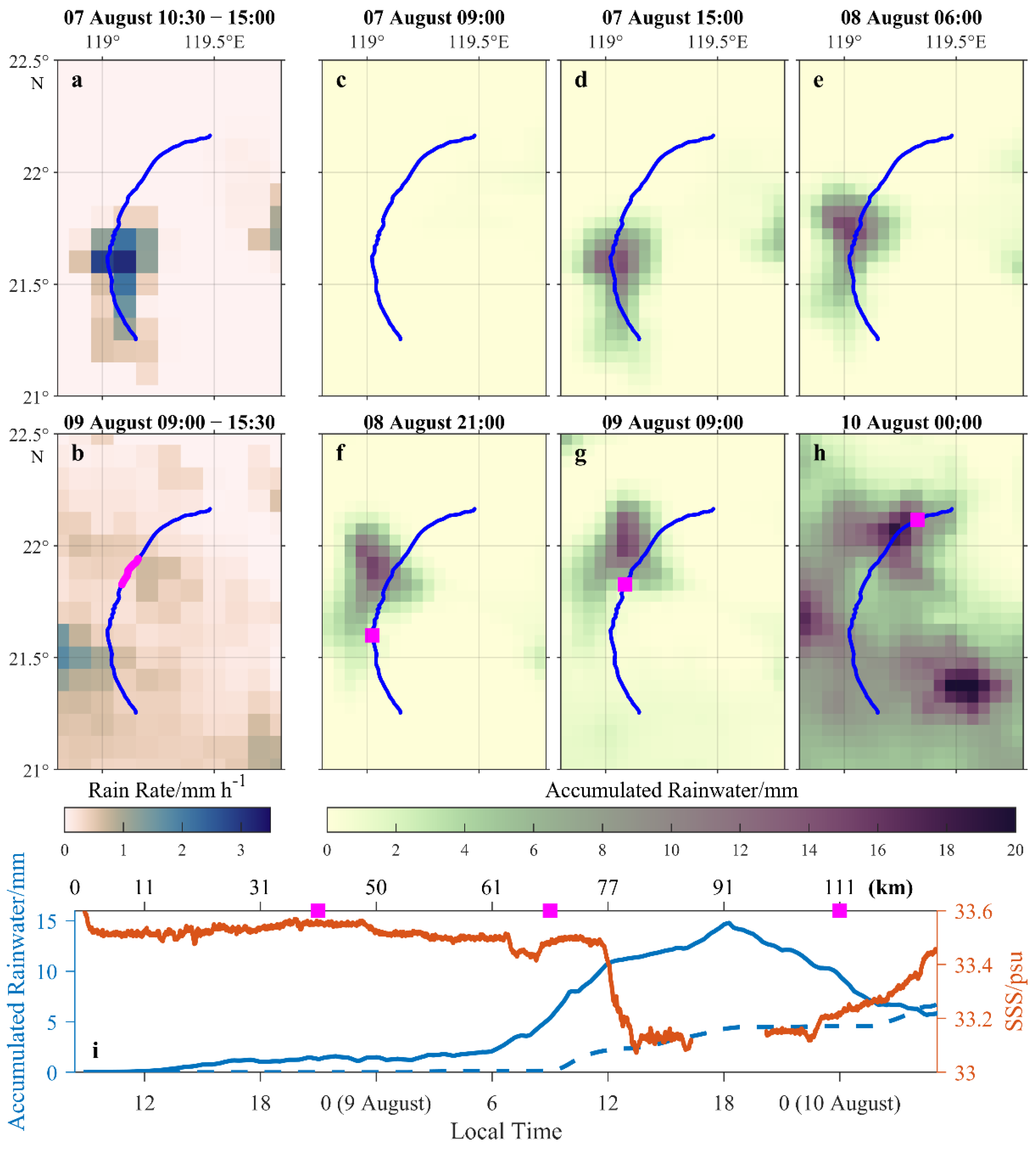
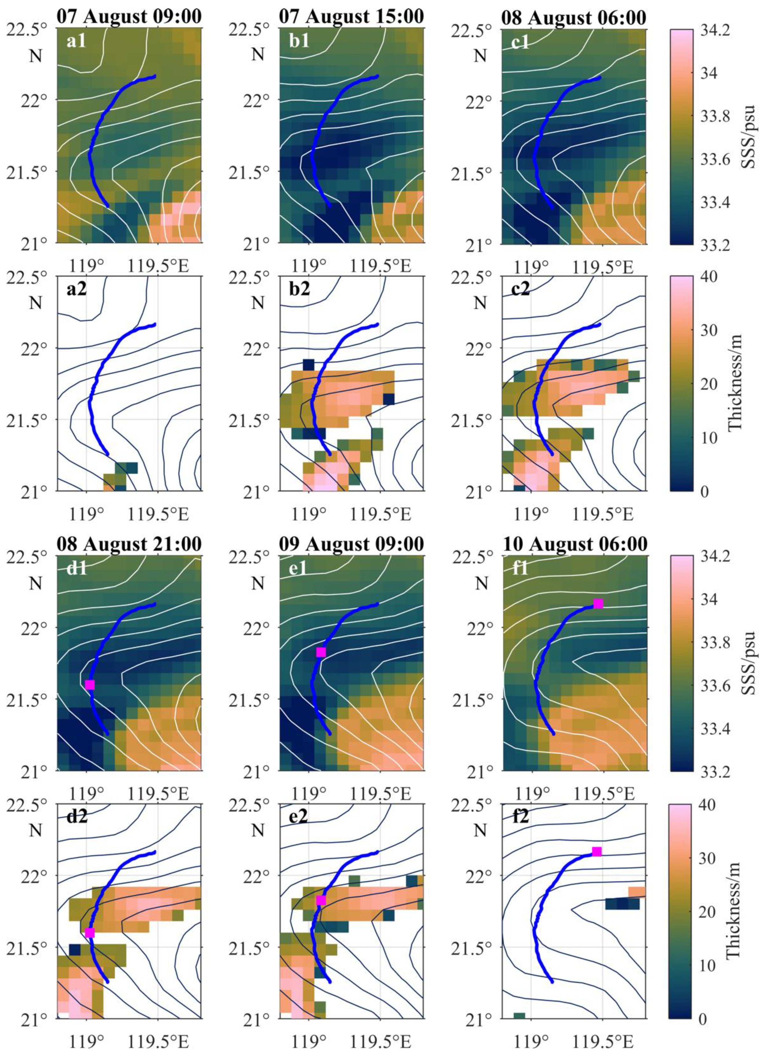
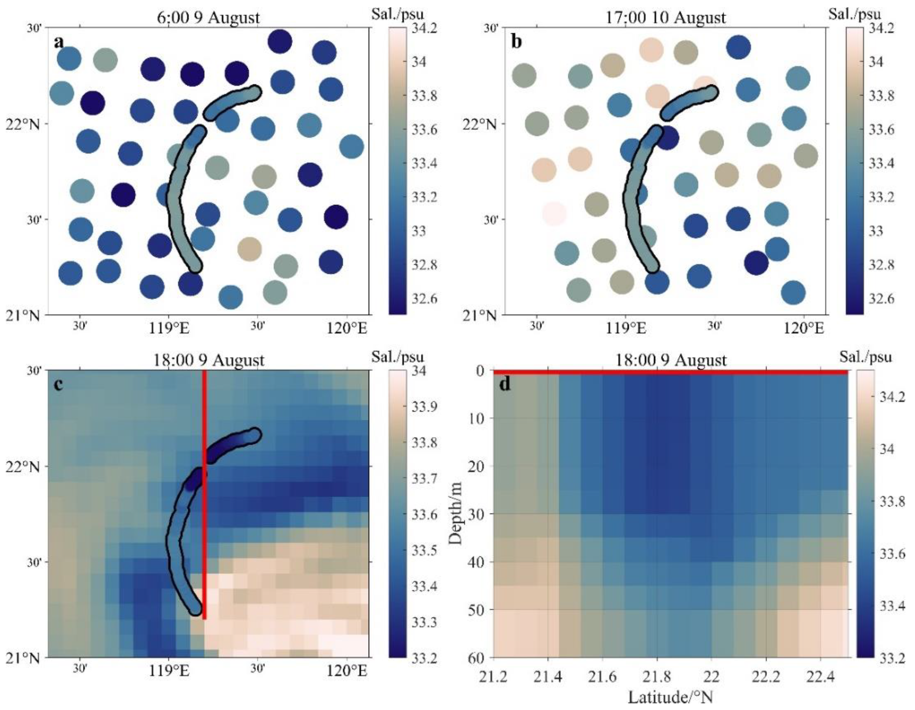
3.2. Origin and Distribution of the LSP

From satellite precipitation data, there were two rainfall events that may have contributed to the formation of the LSP (Figure 4a,b): the first one (10:30–15:00 on 7 August) and the latter one (9:00–15:30 on 9 August). The former was much heavier than the latter. To study the origin and horizontal evolution of the LSP, as well as the contributions of those two rainfall events, we tracked the Lagrange particles and calculated the rainfall carried by those particles based on surface current data (combining geostrophic flows with the Ekman currents) and the satellite data of the precipitation. R_PTS combined two effects: advection contribution and accumulation contribution. The particles were advected by the background currents and carried the “falling raindrops” along the way (i.e., moving rain gauges). The results are shown in Figure 4c–h. The rainwater pool was formed by the first heavy rainfall before we started the transect observations and drifted northeast under the advection of surface flows, and finally, it was observed near the anticyclonic eddy core. As for the R/V, it crossed the rainwater pool and encountered the second rainfall event (Figure 3b,c). To compare the SSS measured by shipboard instruments and the results from PTS, we interpolated R_PTS into the R/V track and thus got “measured” accumulated rainwater by shipboard R_PTS·ship. There is a high correlation between the measured SSS and R_PTS·ship at the location of the R/V during the observation period (correlation coefficient R = −0.90, and significance value p < 0.05). R_PTS·ship (considering horizontal advection under the background currents) was three times larger than R_local (not considering horizontal advection under the background currents) (Figure 4i), suggesting that the latter rainfall event we encountered during the observation (9:00–15:30 on 9 August) cannot explain the observed LSP. This suggests that it was the previous rainfall event (10:30–15:00 on 7 August) that formed the LSP, and its horizontal distribution and evolution were decided by horizontal advection of the surface flow.

The three-dimensional structure of the LSP was further studied using HYCOM Analysis data (the reason is discussed in Appendix A). By selecting 33.35 psu as the threshold, we defined the depth with a salinity less than this threshold as the LSP region. Figure 5 shows the evolution of the LSP. A bowl-like structure of the LSP was formed at 15:00 on 7 August after the former rainfall, showing a thick center (about 30 m) and a thin edge (Figure 5(a1,b1,a2,b2)). It then slowly drifted northwest (Figure 5(c1–e1,c2–e2)), consistent with the PTS (Figure 4c–h). The difference is that the size of the LSP from the HYCOM Analysis data was progressively smaller and disappeared on 10 August since the low-salinity water was mixed or advected by surrounding water in the simulations. The LSP spanned about 3 days according to the analysis based on the HYCOM Analysis data. It may have existed longer in the real ocean since most numerical simulations suffer from the problem of overmixing [44].

These results from both PTS and HYCOM Analysis data agreed well with the observations. As shown in Figure 6a–d, the bowl-like low-salinity/density layer was well correlated with R_PTS·ship. Considering that it was unlikely the R/V crossed the exact center of the PTS, the diameter of the LSP was at least 45 km from the CTD section. Compared with field observations, the HYCOM Analysis data provided good estimates of the LSP thickness (Figure 5(d2–e2) and Figure 6c).

Combining the results from the PTS and HYCOM output analyses, we conclude that the observed LSP evolved from the heavy rainfall event two days before (10:30–15:00 on 7 August). Horizontal advection brought the freshwater to the LSP region.

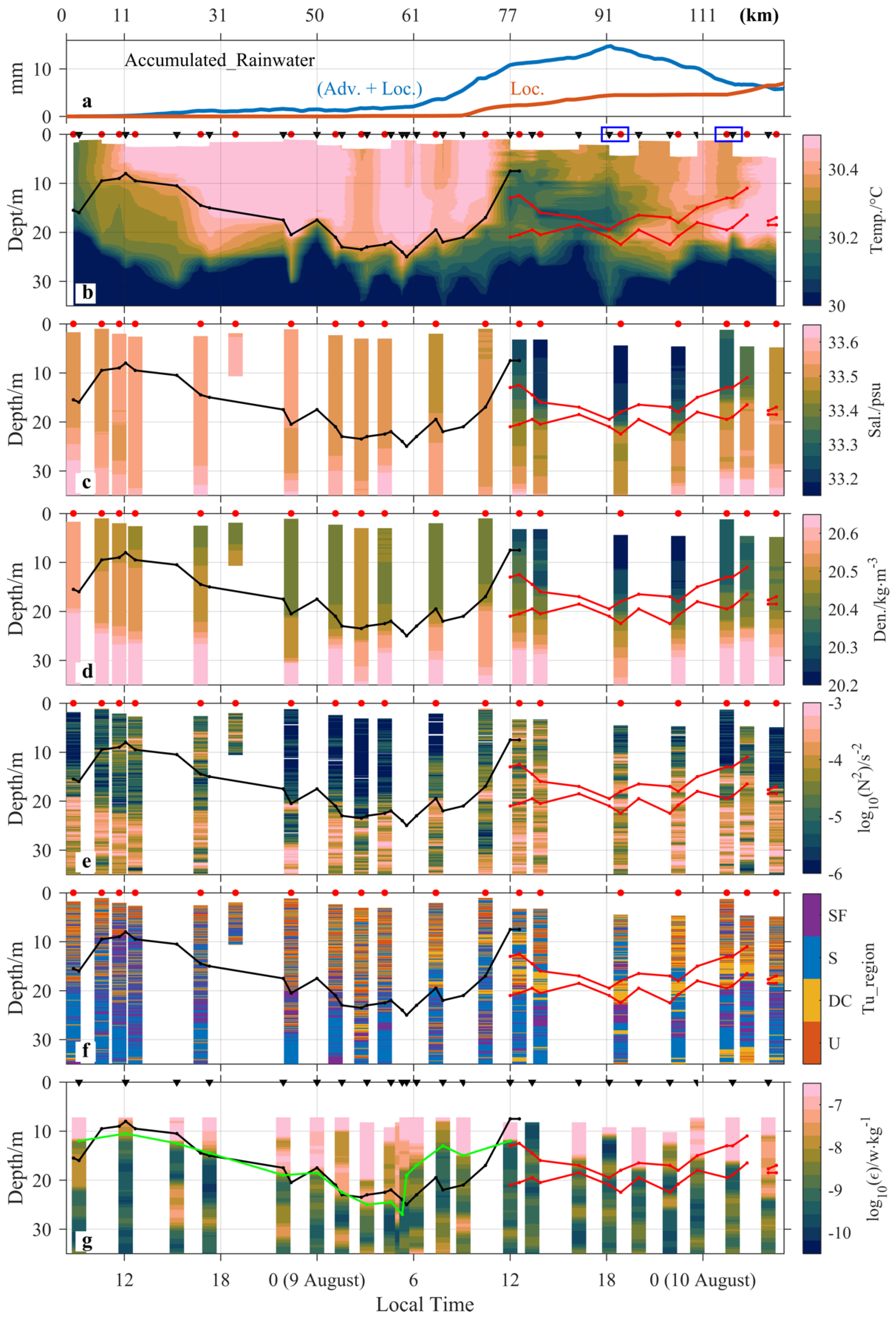
3.3. Vertical Evolution of the LSP

In general, in the absence of rainfall, diurnal solar heating (temperature) dominates the stratification in the mixed layer. Daytime heating makes the surface layer warm, light and stable, forming a warm layer (several meters thick depending on wind and surface waves). However, in the nighttime, when the ocean loses heat, convective overturns occur in the upper layer due to gravity instabilities [45,46]. As a result, the diurnal mixed layer (or convective layer) deepens, entraining more quiescent water upward from below until the diurnal mixed layer depth reaches its maximum depth (i.e., the seasonal mixed layer depth). It is worth noting that typically the salinity has little variation during the whole diurnal cycle.

In this study, the transect before encountering the LSP (before about 12:00 on 9 August) can be roughly regarded as a temporal evolution, and it is the typical temperature-dominated diurnal cycle, as shown in Figure 6. The diurnal mixed layer depth h_ρ (black line in Figure 6) is calculated according to the 0.2 °C temperature criteria relative to the temperature at the surface, given that density variation is dominated by that of the temperature [47,48]. The active mixing layer depth h_ε can be a good proxy for the depth of the diurnal mixed layer depth. It is because convective instabilities at nighttime can be indicated by enhanced turbulent dissipation. Here, h_ε is defined as the depth where the TKE dissipation rate decreases to an assumed background value (i.e., 10⁻⁹ W/kg) [49,50]. The two depths, i.e., h_ρ and h_ε, agreed well with each other. These depths increased as heat lost at the sea surface from ~17:15 on 8 August (Figure 5a and Figure 6). Finally, the active mixing layer depth developed to the depth of 25 m at ~6:00 on 9 August as shown in Figure 6. Therefore, 25 m could be regarded as the maximum depth of nocturnal convection without the influence of LSP in our case study.

After the LSP was formed by the rainfall on 7 August (Figure 4d), nocturnal convection occurred due to nighttime cooling, although salinity dominated the stratification. After sufficient time (2 days) for the development of nocturnal convection, the LSP expanded deeper, reaching a thickness ~20 m (according to the 33.35 psu salinity criteria, not shown here) until it was captured by the R/V on 9 August. As for the local (second) rainfall, it only affected the salinity anomaly in the upper 10 m. This is evidenced by the double-halocline structure in the salinity profile at 18:53 on 9 August (Figure 7a, ~8 h after the local rainfall). Previous studies using numerical simulations have shown that the rain-induced fresh lens can reach a depth of ~5 m after about 4 h [1,2], similar to our observations. It was the first heavy rainfall that caused the 20 m thick LSP via nocturnal convection. However, it did not reach the previous maximum depth (25 m) due to inhibition by the strong haline stratification in the LSP base.

3.4. The Impact of the LSP: The Temperature Inversion Layer

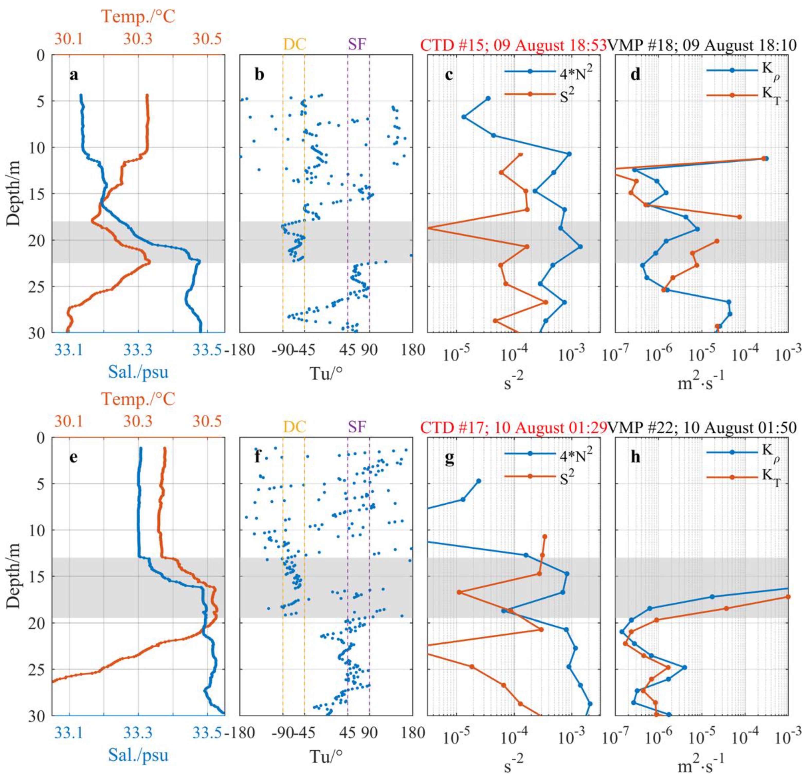
3.4.1. Features of the Temperature Inversion Layer

Previous studies have shown that the temperature and salinity structures of LSPs are highly complex [11,51,52]. Significant thermohaline complexities were also observed during the cruise. The temperature inversion layer (hereafter inversion layer) has been detected directly below the LSP bottom in the temperature profiles (including both CTD and VMP profiles). Its boundaries are marked as two red lines in Figure 6. The upper boundary of the inversion layer is essentially the LSP bottom, and the lower boundary is the base of the seasonal mixed layer. The thickness of the inversion layer ranges between 2 and 8 m, and the temperature difference varies from −0.2 to −0.1 °C. Despite the temperature being reversed, the inversion layer is stable as the vertical gradient of the salinity is much higher (0.1 ± 0.05 psu/m) and dominates the stratification. We also calculated the Turner angle, which is an equivalent parameter of overcoming the large range of density ratios [53]. It can be divided into four regions by Tu, including salt fingering (SF, 45° < Tu < 90°), stable (S, −45° < Tu < 45°), diffusive convection (DC, −90° < Tu < −45°) and unstable (U, 90° < Tu or Tu < −90°). Referring to the Turner angle, the inversion layer could be defined as a diffusive convection layer. When cold, freshwater overlies warm, salty water, diffusive convection can occur, which can enhance mixing [54,55,56]. Two typical profiles from the center and edge of the LSP are shown in Figure 7 to indicate the inversion layer.

3.4.2. Formation and Impact of the Temperature Inversion Layer

The appearance and formation of the inversion layer was related to the occurrence of barrier layers in the upper layer, as reported in previous studies [52,57,58,59]. According to the typical profiles in Figure 7e, we detected the existence of a barrier layer, according to its definition of the isothermal layer being deeper than the isopycnic (isohaline) layer [9,10,11]. Here, the barrier layer was between ~13 and ~23 m, based on the criteria using salinity and temperature, respectively. The barrier layer had strong haline stratification between 13 and 17 m, according to the Turner angle in Figure 7f. The strong haline stratification provided a condition to enhance the stability of the water column and compensate for the stability loss due to the increasing temperature with depth. The existence of the barrier layer restricted the heat exchange between the upper and lower layers, maintaining the existence of the cold/fresh LSP over the warm/salt water.

Due to the barrier layer, the water below the LSP can remain stable and warm. However, water temperature above the barrier layer can decrease due to heat loss by nighttime cooling and mixing with cold rainwater. Considering the heat lost at nighttime (−7.46 × 10⁶ J m⁻²), we calculated the temperature change by nighttime cooling ΔT_night = ~−0.18 °C in the upper 10 m. Additionally, the temperature variation due to the mixing of cold rainwater (~0 psu and ~20 °C) and seawater (~33.5 psu and ~30 °C) was ΔT_rain·mixing = ~−0.09 °C within the LSP based on the observed salinity anomaly (~0.3 psu). The two values of temperature variation (~−0.18 °C, ~−0.09 °C) agreed with the observation of the temperature inversion layer with a value of −0.2–−0.1 °C. Therefore, surface cooling at the basis of the barrier layer was the main reason for the formation of the temperature inversion in our observation.

The existence of the temperature inversion layer can induce diffusive convection. Within the inversion layer, S² was smaller than 4N², suggesting an unlikely possibility of shear instability (Figure 6 and Figure 7). By contrast, the vertical structure of cooler/fresher overlying water warmer/saltier water (−90° < Tu < −45°) provided favorable conditions for diffusive convection. The diapycnal diffusivity for heat (K_T) was around one order of magnitude larger than the diapycnal diffusivity for density (K_ρ), providing the evidence of significantly enhanced mixing for heat by diffusive convection than by shear turbulence within the inversion layer. Actually, similar to the observation of Walesby et al. [15], the faint staircase-like structure was detected in the inversion layer of several T/S profiles from CTD and VMP (not shown), which also indicated the existence of diffusive convection.

4. Conclusions

Treating the R/V as a drifter affected by both ocean current and the wind, we conducted quasi-Lagrangian field observations along the looping path of the Kuroshio intrusion into the northeastern SCS. The R/V encountered a rainfall event and captured a region with low salinity induced by the rainfall. In this paper, we analyzed the distribution, origin and evolution of the LSP. The main conclusions are summarized as follows.

• The LSP was formed by a previous rainfall event, which injected a large amount of freshwater into the upper ocean. Then the LSP drifted northeastward to our study region. This rainfall event was stronger than the second one, which could not affect the upper ocean to a deeper layer. Therefore, the LSP captured by our observations was attributed to the upstream formation of the Kuroshio loop and tracked by the northeastward advection. The conclusion was supported by both the PTS and HYCOM Analysis data.
• The local rainfall during the field observations only affected the upper 10 m of the water column, according to its double-halocline structure. With good development of nocturnal convection within 2 days, the LSP was mainly formed during the previous rainfall event and finally reached a depth of 20 m. However, the existence of an LSP can inhibit the downward development of convective mixing and limit the maximum depth of nocturnal convection.
• A thin temperature inversion layer formed between the bottom of the LSP and the seasonal mixed layer. The formation of the temperature inversion layer was attributed to the surface cooling at the basis of the barrier layer, where strong salinity stratification hindered vertical heat exchange at the base of the LSP. The stable salinity stratification with temperature inversion provided a favorable condition for developing diffusive convection, which was confirmed by the difference between the diapycnal diffusivities of the density and heat.

The results presented in this paper have important implications for not only regional oceanography but also the climate. In this study, the rain-induced LSP was laterally advected by the Kuroshio looping current or mesoscale eddies. The Kuroshio intrusion brings warm and saline Pacific water into the SCS, while local rainfall changes the salinity in the upper ocean, which may be brought into the western Pacific by the Kuroshio. It is because the rain-induced LSP can maintain in the upper ocean for a couple of days and be transported by ocean circulation. Modified by the monsoon and frequent tropical cyclones, the rainfall in the South China Sea not only affects the local water property but may also contribute to the water exchange between the western Pacific and the SCS and has a climate implication. As a result, in addition to studying the effects of precipitation in the upper ocean at seasonal and climate scales, it is worth a more detailed investigation into the dynamic process and influence of rainfall events in further research.

References

1. Soloviev, A.; Lukas, R. The Near-Surface Layer of the Ocean: Structure, dynamics and applications; Springer: New York, NY, USA, 2013. [Google Scholar]
2. Drushka, K.; Asher, W.E.; Ward, B.; Walesby, K. Understanding the formation and evolution of rain-formed fresh lenses at the ocean surface. J. Geophys. Res. Ocean. 2016, 121, 2673–2689. [Google Scholar] [CrossRef] [Green Version]
3. Soloviev, A.; Lukas, R. Observation of Spatial Variability of Diurnal Thermocline and Rain-Formed Halocline in the Western Pacific Warm Pool. J. Phys. Oceanogr. 1996, 26, 2529–2538. [Google Scholar] [CrossRef] [Green Version]
4. Price, J.F. Observations of a Rain-Formed Mixed Layer. J. Phys. Oceanogr. 1979, 9, 643–649. [Google Scholar] [CrossRef] [Green Version]
5. Anderson, S.P.; Weller, R.A.; Lukas, R.B. Surface Buoyancy Forcing and the Mixed Layer of the Western Pacific Warm Pool: Observations and 1D Model Results. J. Clim. 1996, 9, 3056–3085. [Google Scholar] [CrossRef]
6. Webster, P.J.; Clayson, C.A.; Curry, J.A. Clouds, Radiation, and the Diurnal Cycle of Sea Surface Temperature in the Tropical Western Pacific. J. Clim. 1996, 9, 1712–1730. [Google Scholar] [CrossRef]
7. Wijesekera, H.W.; Paulson, C.A.; Huyer, A. The Effect of Rainfall on the Surface Layer during a Westerly Wind Burst in the Western Equatorial Pacific. J. Phys. Oceanogr. 1999, 29, 612–632. [Google Scholar] [CrossRef]
8. Hughes, K.G.; Moum, J.N.; Shroyer, E.L. Evolution of the Velocity Structure in the Diurnal Warm Layer. J. Phys. Oceanogr. 2020, 50, 615–631. [Google Scholar] [CrossRef]
9. Lukas, R.; Lindstrom, E. The mixed layer of the western equatorial Pacific Ocean. J. Geophys. Res. Earth Surf. 1991, 96, 3343–3357. [Google Scholar] [CrossRef]
10. Cronin, M.; McPhaden, M.J. Barrier layer formation during westerly wind bursts. J. Geophys. Res. Ocean. 2002, 107, SRF 21-1–SRF 21-12. [Google Scholar] [CrossRef]
11. Katsura, S.; Sprintall, J. Seasonality and Formation of Barrier Layers and Associated Temperature Inversions in the Eastern Tropical North Pacific. J. Phys. Oceanogr. 2020, 50, 791–808. [Google Scholar] [CrossRef]
12. Katsura, S.; Sprintall, J.; Bingham, F.M. Upper Ocean Stratification in the Eastern Pacific During the SPURSField Campaign. J. Geophys. Res. Ocean. 2021, 126, e2020JC016591. [Google Scholar] [CrossRef]
13. Bingham, F.M.; Li, Z.; Katsura, S.; Sprintall, J. Barrier Layers in a High-Resolution Model in the Eastern Tropical Pacific. J. Geophys. Res. Ocean. 2020, 125, e2020JC016643. [Google Scholar] [CrossRef]
14. Vialard, J.; Delecluse, P. An OGCM Study for the TOGA Decade. Part I: Role of Salinity in the Physics of the Western Pacific Fresh Pool. J. Phys. Oceanogr. 1998, 28, 1071–1088. [Google Scholar] [CrossRef]
15. Walesby, K.; Vialard, J.; Minnett, P.J.; Callaghan, A.H.; Ward, B. Observations indicative of rain-induced double diffusion in the ocean surface boundary layer. Geophys. Res. Lett. 2015, 42, 3963–3972. [Google Scholar] [CrossRef]
16. Soloviev, A.; Lukas, R. Sharp Frontal Interfaces in the Near-Surface Layer of the Ocean in the Western Equatorial Pacific Warm Pool. J. Phys. Oceanogr. 1997, 27, 999–1017. [Google Scholar] [CrossRef]
17. Soloviev, A.; Lukas, R.; Matsuura, H. Sharp frontal interfaces in the near-surface layer of the tropical ocean. J. Mar. Syst. 2002, 37, 47–68. [Google Scholar] [CrossRef]
18. Soloviev, A.; Matt, S.; Fujimara, A. Three-Dimensional Dynamics of Freshwater Lenses in the Ocean’s Near-Surface Layer. Oceanogr. Wash. DC 2015, 28, 142–149. [Google Scholar] [CrossRef] [Green Version]
19. Vinogradova, N.; Lee, T.; Boutin, J.; Drushka, K.; Fournier, S.; Sabia, R.; Stammer, D.; Bayler, E.; Reul, N.; Gordon, A.; et al. Satellite Salinity Observing System: Recent Discoveries and the Way Forward. Front. Mar. Sci. 2019, 6, 243. [Google Scholar] [CrossRef]
20. Drushka, K.; Asher, W.E.; Sprintall, J.; Gille, S.T.; Hoang, C. Global Patterns of Submesoscale Surface Salinity Variability. J. Phys. Oceanogr. 2019, 49, 1669–1685. [Google Scholar] [CrossRef]
21. Drushka, K.; Asher, W.; Jessup, A.; Thompson, E.; Iyer, S.; Clark, D. Capturing Fresh Layers with the Surface Salinity Profiler. Oceanography 2019, 32, 76–85. [Google Scholar] [CrossRef]
22. Laxague, N.J.M.; Zappa, C.J. The Impact of Rain on Ocean Surface Waves and Currents. Geophys. Res. Lett. 2020, 47, e2020GL087287. [Google Scholar] [CrossRef] [Green Version]
23. Lin, Y.-C.; Oey, L.-Y. Rainfall-enhanced blooming in typhoon wakes. Sci. Rep. 2016, 6, 31310. [Google Scholar] [CrossRef] [PubMed] [Green Version]
24. Yuan, Z.; Liu, D.; Masque, P.; Zhao, M.; Song, X.; Keesing, J.K. Phytoplankton Responses to Climate-Induced Warming and Interdecadal Oscillation in North-Western Australia. Paleoceanogr. Paleoclimatol. 2020, 35, e2019PA003712. [Google Scholar] [CrossRef]
25. Ho, D.T.; Bliven, L.F.; Wanninkhof, R.; Schlosser, P. The effect of rain on air-water gas exchange. Tellus B Chem. Phys. Meteorol. 1997, 49, 149–158. [Google Scholar] [CrossRef] [Green Version]
26. Takagaki, N.; Komori, S. Effects of rainfall on mass transfer across the air-water interface. J. Geophys. Res. Ocean. 2007, 112, C06006. [Google Scholar] [CrossRef]
27. Zappa, C.J.; Ho, D.T.; McGillis, W.R.; Banner, M.L.; Dacey, J.W.H.; Bliven, L.F.; Ma, B.; Nystuen, J. Rain-induced turbulence and air-sea gas transfer. J. Geophys. Res. Ocean. 2009, 114, C06006. [Google Scholar] [CrossRef] [Green Version]
28. Ho, D.T.; Schlosser, P.; Hendricks, M.B.; Zappa, C.J.; McGillis, W.R.; Bliven, L.F.; Ward, B.; Dacey, J.W.H. Influence of rain on air-sea gas exchange: Lessons from a model ocean. J. Geophys. Res. Ocean. 2004, 109. [Google Scholar] [CrossRef]
29. Liu, W.T.; Xie, X. Spacebased observations of the seasonal changes of south Asian monsoons and oceanic responses. Geophys. Res. Lett. 1999, 26, 1473–1476. [Google Scholar] [CrossRef] [Green Version]
30. Xie, S.-P.; Xu, H.; Saji, N.H.; Wang, Y.; Liu, W.T. Role of Narrow Mountains in Large-Scale Organization of Asian Monsoon Convection. J. Clim. 2006, 19, 3420–3429. [Google Scholar] [CrossRef]
31. Zeng, L.L.; Chen, J.; Shi, P. Response of upper ocean salinity to precipitation during summer monsoon. J. Trop. Oceanogr. 2007, 26, 11–17. [Google Scholar]
32. Zeng, L.; Du, Y.; Xie, S.-P.; Wang, D. Barrier layer in the South China Sea during summer 2000. Dyn. Atmos. Ocean. 2009, 47, 38–54. [Google Scholar] [CrossRef] [Green Version]
33. Guo, J.; Chen, X.Y.; Zhang, Y.L. Factors Influencing the Seasonal Variations of Mixed Layer Salinity in the South China Sea. Adv. Mar. Sci. 2013, 31, 180–187. [Google Scholar]
34. Roget, E.; Lozovatsky, I.; Sanchez, X.; Figueroa, M. Microstructure measurements in natural waters: Methodology and applications. Prog. Oceanogr. 2006, 70, 126–148. [Google Scholar] [CrossRef]
35. Bluteau, C.E.; Lueck, R.G.; Ivey, G.; Jones, N.L.; Book, J.W.; Rice, A.E. Determining Mixing Rates from Concurrent Temperature and Velocity Measurements. J. Atmos. Ocean. Technol. 2017, 34, 2283–2293. [Google Scholar] [CrossRef]
36. Osborn, T.R. Estimates of the Local Rate of Vertical Diffusion from Dissipation Measurements. J. Phys. Oceanogr. 1980, 10, 83–89. [Google Scholar] [CrossRef] [Green Version]
37. Gregg, M.; D’Asaro, E.; Riley, J.; Kunze, E. Mixing Efficiency in the Ocean. Annu. Rev. Mar. Sci. 2018, 10, 443–473. [Google Scholar] [CrossRef]
38. Osborn, T.R.; Cox, C.S. Oceanic fine structure. Geophys. Fluid Dyn. 1972, 3, 321–345. [Google Scholar] [CrossRef]
39. Hou, A.Y.; Kakar, R.K.; Neeck, S.; Azarbarzin, A.A.; Kummerow, C.D.; Kojima, M.; Oki, R.; Nakamura, K.; Iguchi, T. The global precipitation measurement mission. Bull. Am. Meteorol. Soc. 2014, 95, 701–722. [Google Scholar] [CrossRef]
40. Rio, M.-H.; Mulet, S.; Picot, N. Beyond GOCE for the ocean circulation estimate: Synergetic use of altimetry, gravimetry, and in situ data provides new insight into geostrophic and Ekman currents. Geophys. Res. Lett. 2014, 41, 8918–8925. [Google Scholar] [CrossRef]
41. Lange, M.; Sebille, E.V. Parcels v0. 9: Prototyping a Lagrangian ocean analysis framework for the petascale age. Geosci. Model Dev. 2017, 10, 4175–4186. [Google Scholar] [CrossRef] [Green Version]
42. Delandmeter, P.; van Sebille, E. The Parcels v2.0 Lagrangian framework: New field interpolation schemes. Geosci. Model Dev. 2019, 12, 3571–3584. [Google Scholar] [CrossRef] [Green Version]
43. Skofronick-Jackson, G.; Petersen, W.A.; Berg, W.; Kidd, C.; Stocker, E.F.; Kirschbaum, D.B.; Kakar, R.; Braun, S.A.; Huffman, G.J.; Iguchi, T.; et al. The Global Precipitation Measurement (GPM) Mission for Science and Society. Bull. Am. Meteorol. Soc. 2017, 98, 1679–1695. [Google Scholar] [CrossRef] [PubMed]
44. Robertson, R.; Hartlipp, P. Surface wind mixing in the Regional Ocean Modeling System (ROMS). Geosci. Lett. 2017, 4, 1–11. [Google Scholar] [CrossRef] [PubMed] [Green Version]
45. Brainerd, K.E.; Gregg, M.C. Diurnal restratification and turbulence in the oceanic surface mixed layer: 1. Observations. J. Geophys. Res. Earth Surf. 1993, 98, 22645–22656. [Google Scholar] [CrossRef]
46. Lombardo, C.P.; Gregg, M.C. Similarity scaling of viscous and thermal dissipation in a convecting surface boundary layer. J. Geophys. Res. Earth Surf. 1989, 94, 6273–6284. [Google Scholar] [CrossRef]
47. Kara, A.B.; Rochford, P.A.; Hurlburt, H.E. An optimal definition for ocean mixed layer depth. J. Geophys. Res. Earth Surf. 2000, 105, 16803–16821. [Google Scholar] [CrossRef]
48. De Boyer Montegut, C.; Madec, G.; Fischer, A.S.; Lazar, A.; Iudicone, D. Mixed layer depth over the global ocean: An examination of profile data and a profile-based climatology. J. Geophys. Res. Ocean. 2004, 109, C12003. [Google Scholar] [CrossRef]
49. Sutherland, G.; Reverdin, G.; Marié, L.; Ward, B. Mixed and mixing layer depths in the ocean surface boundarylayer under conditions of diurnal stratification. Geophys. Res. Lett. 2014, 41, 8469–8476. [Google Scholar] [CrossRef] [Green Version]
50. Brainerd, K.E.; Gregg, M.C. Surface mixed and mixing layer depths. Deep Sea Res. I 1995, 42, 1521–1543. [Google Scholar] [CrossRef]
51. Moulin, A.J.; Moum, J.N.; Shroyer, E.L.; Hoecker-Martínez, M. Freshwater Lens Fronts Propagating as Buoyant Gravity Currents in the Equatorial Indian Ocean. J. Geophys. Res. Ocean. 2021, 126, e2021JC017186. [Google Scholar] [CrossRef]
52. Thadathil, P.; Suresh, I.; Gautham, S.; Kumar, S.P.; Lengaigne, M.; Rao, R.R.; Neetu, S.; Hegde, A. Surface layer temperature inversion in the Bay of Bengal: Main characteristics and related mechanisms. J. Geophys. Res. Ocean. 2016, 121, 5682–5696. [Google Scholar] [CrossRef]
53. Ruddick, B. A practical indicator of the stability of the water column to double-diffusive activity. Deep Sea Res. Part A Oceanogr. Res. Pap. 1983, 30, 1105–1107. [Google Scholar] [CrossRef]
54. Radko, T. Double-Diffusive Convection; Springer: New York, NY, USA, 2013. [Google Scholar]
55. Nagai, T.; Inoue, R.; Tandon, A.; Yamazaki, H. Evidence of enhanced double-diffusive convection below the main stream of the Kuroshio Extension. J. Geophys. Res. Ocean. 2015, 120, 8402–8421. [Google Scholar] [CrossRef] [Green Version]
56. George, J.V.; Vinayachandran, P.N.; Nayak, A.A. Enhanced Double-Diffusive Salt Flux from the High-Salinity Core of Arabian Sea Origin Waters to the Bay of Bengal. J. Phys. Oceanogr. 2021, 51, 505–518. [Google Scholar] [CrossRef]
57. Sprintall, J.; Cronin, M.F. Upper ocean vertical structure. Encycl. Ocean Sci. 2001, 6, 3120–3129. [Google Scholar]
58. Thadathil, P.; Gopalakrishna, V.; Muraleedharan, P.; Reddy, G.; Araligidad, N.; Shenoy, S. Surface layer temperature inversion in the Bay of Bengal. Deep Sea Res. Part I Oceanogr. Res. Pap. 2002, 49, 1801–1818. [Google Scholar] [CrossRef]
59. Sprintall, J. SIDEBAR. Upper-Ocean Salinity Stratification During SPURS-2. Oceanography 2019, 32, 40–41. [Google Scholar] [CrossRef]
Figure 1. The study region, surface geostrophic current and the sampling stations during the field observations. (a) The surface geostrophic currents (arrows) and the corresponding absolute dynamic topography (colored contours, with a contour interval of 0.05 m) from Archiving, Validation, and Interpretation of Satellite Oceanographic data (AVISO). The blue curve indicates the R/V track. (b) The sampled CTD (red dots, #1−#19) and VMP stations (black triangles, #1−#23) shown in a zoomed area indicated by the red rectangle in (a). Colored contours are the same as in (a).
Remotesensing 14 02030 g001
Figure 2. The drifting velocity of the R/V (blue arrows and lines), surface velocity (red arrows and lines) and the wind velocity (yellow arrows and lines). (a) Velocity (arrows). (b) Speed. (c) Direction. 0° (180°) means due north (south) and 90° (−90°) means due east (west). The gray lines indicate wind direction plus 45°.
Remotesensing 14 02030 g002
Figure 3. (a) Air temperature (blue lines) and net surface heat flux (red lines). (b) Rainfall rate from the R/V’s AWS (blue lines) and GPM (red lines). (c) Near sea surface salinity (blue lines) and temperature (red lines) from SBE-21. Rectangles indicate salinity (blue) and temperature (red) from CTD profiles at ~5 m depth. Vertical axes are scaled by the thermal expansion and haline contraction coefficients, respectively, so that fluctuations of temperature and salinity of equal size imply identical contributions to the density.
Remotesensing 14 02030 g003
Figure 4. (a,b) The mean rain rate based on GPM data during the two rainfall events. The magenta lines indicate the R/V track during the rain periods. (ch) RPTS in different times. The magenta squares indicate the position of the R/V. (i) RPTS·ship (blue solid lines) and Rlocal (blue dash lines). Red lines indicate the sea surface salinity from SBE-21. The blue curve in (ah) indicates the R/V track during the observation. The magenta squares in (i) indicate the same time as in (fh).
Remotesensing 14 02030 g004
Figure 5. (a1f1) Sea surface salinity (colored) and sea surface height (white contours, with a contour interval of 0.025 m) from the HYCOM Analysis data. (a2f2) Thickness of the low-salinity water layer (colored, according to the 33.35 psu salinity criteria) and sea surface height (black contours, with a contour interval of 0.025 m) from HYCOM Analysis data. The blue curve indicates the R/V track during the observation. The magenta squares indicate the R/V position.
Remotesensing 14 02030 g005
Figure 6. (a) RPTS·ship (blue solid lines) and Rlocal (red solid lines). Distance coordinates were added according to the R/V track in space. (bg) Vertical profiles during the cruise observations. Black triangles indicate VMP profiles. Red dots indicate CTD profiles. (b) Temperature. (c) Salinity. (d) Potential density anomaly. (e) Squared buoyancy frequency (N2). (f) Double-diffusive stability based on the Turner angle. (g) TKE dissipation rate. Red lines in (bg) indicate the depth range of the temperature inversion layer. Black lines in (bg) indicate the base of the diurnal mixed layer according to the 0.2 °C temperature criteria. Green lines in (g) indicate the base of the active mixing layer according to the 10−9 W/kg background dissipation rate. Blue boxes in (b) indicate the typical profiles shown in Figure 7.
Remotesensing 14 02030 g006
Figure 7. Two typical profiles as the two blue boxes marked in Figure 6b. Gray shadings indicate the temperature inversion layer. (a,e) Temperature (red lines) and salinity (blue lines). (b,f) Turner angle. Yellow dashed lines indicate the diffusive convection (DC) region. Purple dashed lines indicate the salt finger (SF) region. (c,g) The squared buoyancy frequency (N2) and the shear squared (S2). N2 has been multiplied by a factor of 4 to comparison with the critical Richardson number (Ri = 0.25 or, equivalently, 4N2 = S2). (d,h) The diapycnal diffusivities of density (Kρ) and heat (KT).
Remotesensing 14 02030 g007