
A Fast Inference Vision Transformer for Automatic Pavement Image Classification and Its Visual Interpretation Method


1
Department of Roadway Engineering, School of Transportation, Southeast University, Nanjing 211189, China
2
National Demonstration Center for Experimental Road and Traffic Engineering Education, Southeast University, Nanjing 211189, China
*
Author to whom correspondence should be addressed.
Remote Sens. 2022, 14(8), 1877; https://doi.org/10.3390/rs14081877
Submission received: 24 March 2022
/
Revised: 8 April 2022
/
Accepted: 11 April 2022
/
Published: 13 April 2022
(This article belongs to the Special Issue Road Extraction and Distress Assessment by Spaceborne, Airborne and Terrestrial Platforms)
Abstract
:Traditional automatic pavement distress detection methods using convolutional neural networks (CNNs) require a great deal of time and resources for computing and are poor in terms of interpretability. Therefore, inspired by the successful application of Transformer architecture in natural language processing (NLP) tasks, a novel Transformer method called LeViT was introduced for automatic asphalt pavement image classification. LeViT consists of convolutional layers, transformer stages where Multi-layer Perception (MLP) and multi-head self-attention blocks alternate using the residual connection, and two classifier heads. To conduct the proposed methods, three different sources of pavement image datasets and pre-trained weights based on ImageNet were attained. The performance of the proposed model was compared with six state-of-the-art (SOTA) deep learning models. All of them were trained based on transfer learning strategy. Compared to the tested SOTA methods, LeViT has less than 1/8 of the parameters of the original Vision Transformer (ViT) and 1/2 of ResNet and InceptionNet. Experimental results show that after training for 100 epochs with a 16 batch-size, the proposed method acquired 91.56% accuracy, 91.72% precision, 91.56% recall, and 91.45% F1-score in the Chinese asphalt pavement dataset and 99.17% accuracy, 99.19% precision, 99.17% recall, and 99.17% F1-score in the German asphalt pavement dataset, which is the best performance among all the tested SOTA models. Moreover, it shows superiority in inference speed (86 ms/step), which is approximately 25% of the original ViT method and 80% of some prevailing CNN-based models, including DenseNet, VGG, and ResNet. Overall, the proposed method can achieve competitive performance with fewer computation costs. In addition, a visualization method combining Grad-CAM and Attention Rollout was proposed to analyze the classification results and explore what has been learned in every MLP and attention block of LeViT, which improved the interpretability of the proposed pavement image classification model.
1. Introduction
Cracks are common pavement distress caused by vehicle loading and environmental conditions. Pavement cracking can cause damage to pavement structures, and the area of pavement structure damage can increase over time, affecting the performance of the pavement. Therefore, the timely detection and monitoring of pavement cracks and other distress is essential for road maintenance [1,2].
The traditional manual pavement distress detection method is inefficient and significantly affected by subjective factors, restricting the development of maintenance intelligence. In response to such problems, benefiting from the development of artificial intelligence technology, researchers have continuously applied the latest image-processing methods to pavement disease recognition [3]. Deep learning is the state-of-the-art (SOTA) artificial intelligence method. Compared with traditional image-processing and machine-learning methods, complex image preprocessing is not required in deep learning. Deep learning has the characteristics of automatic feature learning, which can significantly improve the efficiency of pavement distress recognition. It is a general trend to collect pavement images using automated detection equipment and adopt advanced algorithms to identify pavement distress [4,5].
Convolutional Neural Network (CNN) has been well established in image recognition among all the deep learning methods in pavement distress identification. Since AlexNet was proposed in 2012 [6], new CNN structures have been introduced every year. Breakthroughs in early CNN structures such as VGG [7] and MSRANet [8] were mainly in larger width and depth, resulting in more neurons and parameters. This may cause overfitting and requires a large number of computation resources. The application of residual blocks significantly improved the efficiency of training a CNN and was widely used in the architectures of some SOTA CNN, such as ResNet [9] and DenseNet [10]. In the last 5 years, extensive research has been conducted and has shown that the application of CNN in pavement distress identification is feasible and scientific. Wang’s research team proposed several CNN-based crack detection models named CrackNet and improved versions [11,12,13]. Because training a CNN is time-consuming, the improvement direction of their proposed models is mainly higher detection accuracy and faster performance. Hou et al. [14] proposed an adaptive, lightweight CNN pavement object classification model named MobileCrack to achieve more efficient training. Ali et al. [15] introduced a customized CNN for concrete crack detection. By comparing existing well-known CNN models, they found that the number of learnable parameters of models can significantly affect the computational time. Kim et al. [16] employed a shallow CNN to acquire higher identification accuracy with minimum computation. All of this research showed that computation time and accuracy are critical for applying deep learning in pavement distress recognition. However, CNNs still have the problem that the lower-level features outside the effective receptive fields cannot be described [17,18]. It is not conducive to making full use of the context information to capture features of images. Continuously stacking deeper convolutional layers can help get more levels of image features, but it will cause a sharp increase in computation.
Recurrent neural networks (RNNs), including LSTM [19] and GRU [20], are also typical deep learning methods. RNNs have the advantage that they can combine contextual information and are widely used in speech recognition. Sequential data are required to conduct the RNN model, which differs from the pavement image dataset. Limited studies about RNN-based pavement image recognition have been completed. Zhang et al. [21] defined the sequence of pixels in an image as the input sequence of RNN. They proposed CrackNet-R for pavement crack detection, which revealed the potential of sequence-based deep learning in pavement image recognition. In the application of computer vision in pavement image recognition, CNNs remain dominant.
Self-attention is a structure to help deal with the problem of parallelization within training examples in recurrent models [22]. A network called Transformer entirely based on attention mechanism and eliminates recurrence and convolutions was proposed to solve the parallel processing of words in a sentence in RNN-based models and achieved considerable success in natural language processing [22,23]. Inspired by the successful application of Transformer in natural language processing, an image classification model that displaced the traditional convolutional networks and was based entirely on Transformer architecture called Vision Transformer (ViT) was initially introduced in computer vision and turned out to have competitive performance in a large-scale image database [24]. Nevertheless, the original ViT model still has some problems, such as its poor generalization ability on inadequate data. Thus, more and more improved versions of ViT-based image recognition methods were proposed recently [25,26,27,28].
A typical Transformer block contains multi-head self-attention, skip connection, and normalization. In terms of pavement image recognition, researchers have also made preliminary attempts to apply Transformer to pavement distress detection. Liu et al. [29] employed a network called CrackFormer using the self-attention modules embedded in the CNN structure. Guo et al. [30] adopted a vision transformer structure to detect the crack boundary and found it precedes several SOTA schemes. These works focus on the edge detection of crack images. Image classification is a fundamental task in deep learning and is the backbone of other complex tasks such as object detection and semantic segmentation. However, deep learning-based object classification in pavement images remains challenging because of the inconspicuous features, low contrast and noisy background, and high economic cost of computation. To solve the above problems, a faster inference vision transformer model called LeViT [31] was applied in pavement object classification in this study. It combined the convolutional operation in the original ViT structure and achieved competitive classification accuracy with a relatively higher processing speed.
On the other hand, as deep learning-based algorithms were once addressed as ‘black box’, the interpretability matters of deep learning have been a problem for many years [32,33]. Moreover, as deep learning models become increasingly complex, it is also becoming increasingly difficult for us to understand our model [34]. To build up trust in the AI-based pavement distress recognition models for engineers, ensuring the ability to understand why a particular prediction is made is critical. Therefore, in our study, a visual interpretation method for both multilayer perceptron (MLP) and self-attention blocks was proposed to better understand the mechanism of the employed deep learning model. Our work is a potential solution for the interpretability matters in deep learning-based pavement distress detection models.
The rest of this paper is structured as follows: Section 2 presents the methodology, including the introduction of the original ViT methods, the overall structure of the LeViT model, visual explanation methods, and the evaluation matrix; Section 3 presents the experimental results of the proposed classification model and the analysis of the visual interpretation results; Section 4 presents the discussion and comparison of other SOTA models; and, finally, Section 5 offers the research conclusion.
2. Methodology and Materials
2.1. Overall Procedure
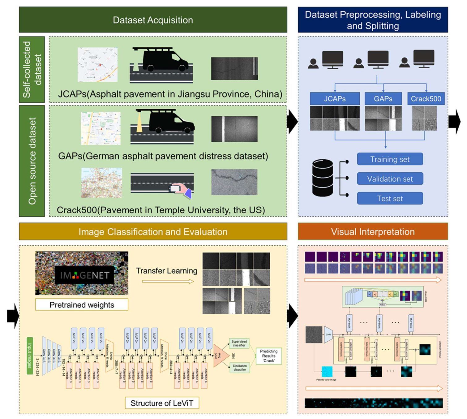
Figure 1 shows the framework of the proposed work. We collected the pavement images from three distinct sources, forming three different datasets for comparison experiments. The original images were then preprocessed to a smaller size that meets the computer training requirements. Next, the three datasets were divided in the ratio of 6:2:2 to form the training set, validation set, and test set, respectively. A transformer-based deep learning approach called LeViT was used to automatically classify the pavement images. During training, pre-trained weights based on the ImageNet were obtained, and then the model was trained based on our datasets using the transfer learning strategy. The proposed method was also compared with other prevailing deep learning networks. Subsequently, a visualization strategy was proposed to visualize the classification results and what has been learned at each layer of our proposed network.
2.2. Data Acquisition
Three different pavement datasets are used in our experiments.
- (1)
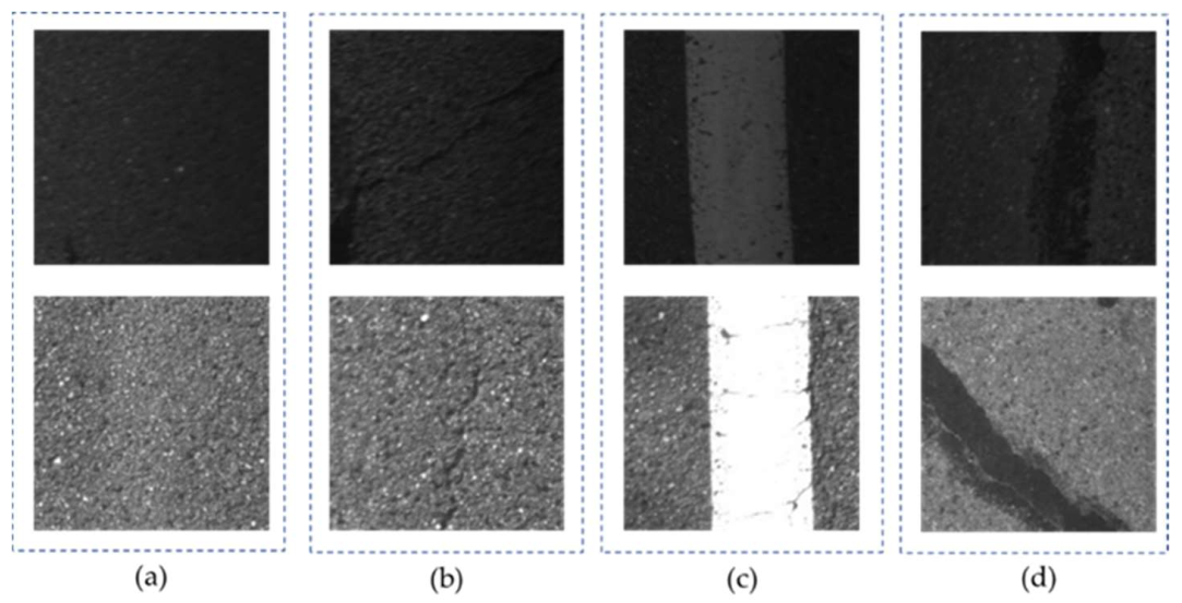
- JCAPs: The first dataset was collected from the multi-functional intelligent road detection vehicle on asphalt pavement on Lanhua Road, Nanjing, Jiangsu Province, China, in April 2018. This multi-functional pavement detection vehicle was equipped with onboard computers and embedded integrated multi-sensor synchronous control units to automatically capture pavement pictures. It took about half an hour for the vehicle to collect the original images. The original data collected were RGB images of 4096 × 2000 pixels. To satisfy the training requirements, the original images were processed to a proper size. First, the original images were horizontally resized to 4000 × 2000 pixels via bilinear interpolation. Then, the resized images were continuously clipped to 400 × 400 pixels. Subsequently, the sub-images were resized to 224 × 224 pixels. To balance the number of images of various samples in the dataset, 1600 images were selected, including 400 pavement background images, pavement marking images, crack images, and sealed crack images. In terms of the crack images, transverse and longitudinal crack images are included in the dataset. This dataset is named as JCAPs. Example images of different classifications in JCAPs are shown in Figure 2. As the images were affected by the equipment and lighting conditions, the original dataset contained road images with good lighting exposure and poor lighting exposure. In addition, the cracks in this image dataset have a relatively smaller width, and the image feature is inconspicuous, which may increase the difficulty of classification for deep learning models.
- (2)
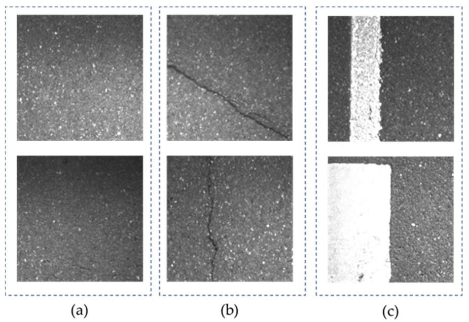
- GAPs: The German Asphalt Pavement Distress (GAPs) dataset is an open-source dataset with various classes of distress using a mobile mapping system. Four-year cycle images are contained in the original GAPs dataset. The resolution of the original images is 1920 × 1080 pixels. More details of the dataset are presented in [35]. We randomly selected several of the original images and cropped the original GAPs images into tiny images with 400 × 400 pixels using the sliding-window method and resized them into 224 × 224 pixels to prevent the problem of running out of memory while computing. A total of 1200 images with the size of 224 × 224 were manually labeled, including 400 pavement background images, pavement marking images, and crack images. Longitudinal and transverse cracking are included in the crack images. Figure 3 shows the example images from the GAPs dataset.
- (3)
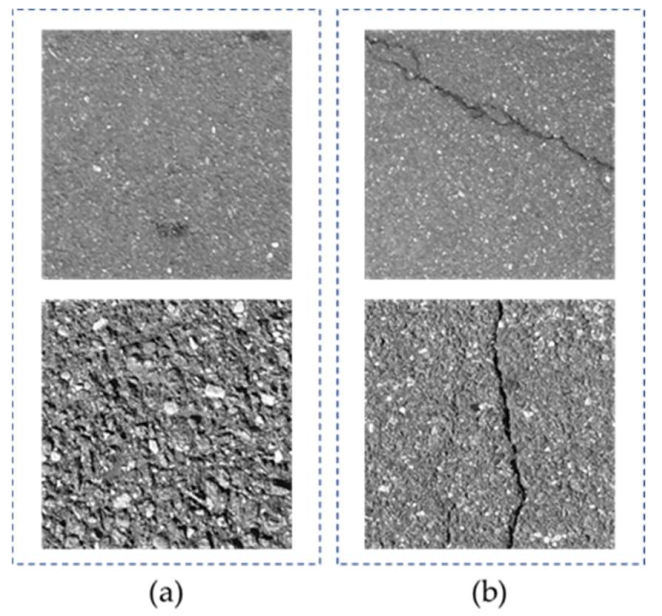
- Crack500: This dataset is also an open-source dataset collected from the main campus of Temple University, Philadelphia, Pennsylvania, U.S. The resolution of the original images in the Crack500 dataset is 2000 × 1500 pixels. More details of the dataset are presented in [36,37]. We also randomly selected several of the original images and cropped the original images into 500 × 500 pixels using the sliding-window method. The tiny images were also resized to 224 × 224 pixels before inputting into the training networks. A total of 2000 images with the size of 224 × 224 were manually categorized, including 1000 pavement background images and 1000 crack images. The crack images include longitudinal and transverse cracks. Figure 4 shows the example preprocessed images in the Crack500 dataset.
In this study, 60% of every dataset was used as the training set for network training, 20% of every dataset was used as the validation set for network validation and monitoring, and 20% was allocated as the test set to evaluate different models. The different classes of samples in the dataset had a balanced distribution. Table 1 describes the distribution of pavement images in each classification in every dataset.
2.3. Vision Transformer
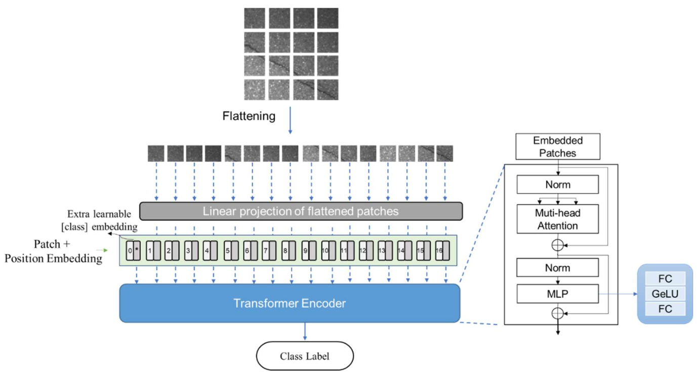
The structure of ViT entirely replaces the convolution operation in image recognition. The original architecture of ViT splits images into patches. Then, the patches are flattened and linear projected into learnable features. To acquire the position information of image patches, position encoding is added to the Patch embedding. Moreover, an extra learnable class embedding, named class token, is also input into the transformer encoder. Layer normalization and two fully connected layers are included in the classifier. The output of the class token is taken as the classification result of the whole network. Figure 5 shows the framework of the original ViT.
Residual connection is applied in the transformer encoder. This structure was first proposed in ResNet [9]. It allows lower layers to directly connect to higher layers and skip one or more middle layers. It does not introduce additional parameters or add computation complexity but can help improve the accuracy with the same computation resources.
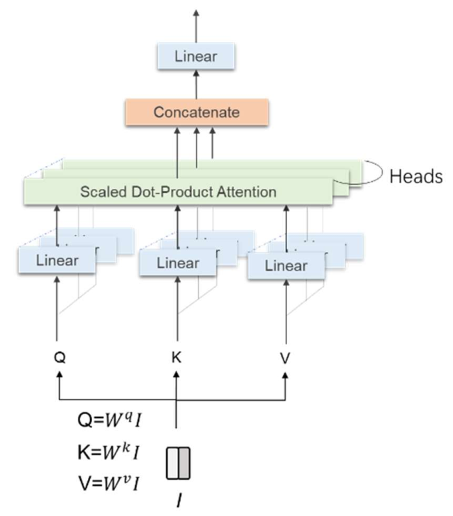
Multi-head attention is the core block in transformer models. The architecture of attention was firstly introduced in 2014 [38]. The neural network can pay more attention to relevant information in input vectors using an attention mechanism. An illustration of the multi-head self-attention is presented in Figure 6. The input vector of embedded patches after normalization is I. By multiplying with three different trainable weight matrices Wq, Wk, and Wv, the input of multi-head attention is query Q, key K, and value V. All of them are linear projected, and then scaled dot-product is applied to calculate attention score, seen in Equation (1) [22], and SoftMax function is used as alignment function, and Equation (2).
![Remotesensing 14 01877 g006]() where dk is the dimension of K. xi is the input activation of attention blocks. n is the dimension of the input vector.
where dk is the dimension of K. xi is the input activation of attention blocks. n is the dimension of the input vector.
Figure 6.
Illustration of multi-head self-attention in Transformers.

Multi-head attention is to conduct different linear transformations by h times to project Q, K, and V. After that, attention results of different heads are concatenated, shown in Equation (3) [22] and Equation (4) [22]:
where , and present learnable weight matrix in the ith head, and h is the number of head.
2.4. Levit Structure
LeViT is a newly developed approach proposed in 2021 [31]. It reintroduced convolutional operations, which replaced some Transformer components to achieve a faster inference speed. The architecture of LeViT is similar to LeNet [39], where the whole network presents a pyramid shape with pooling. Specifically, the difference between LeViT and original ViT can be summarized in the following aspects.
- (1)
- Convolutional layers
The convolution operation is adopted in this network to extract features. Four convolutional layers with the kernel size of 3 × 3 are added to process the input images. After the convolutional layers, a tensor with more channels and smaller width and height is acquired as the input of Transformer Blocks. Batch normalization [40] is used to stabilize the training process. All of the activation function in LeViT is Hardswish, shown in Equation (5) [41]:
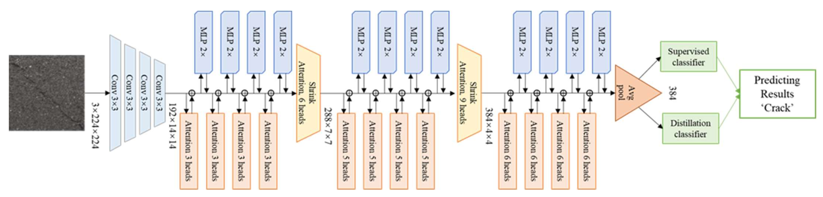
The size of the output feature map of the last convolutional layers is 13 × 13. The number of the channels of the output of the previous convolutional layer determines the input size of the transformer blocks. LeViT-192 represents that the number of channels on the input of transformer stage is 192. The architecture of the LeViT-192 is presented in Figure 7.
- (2)
- Transformer stages
There are three Transformer stages in LeViT. Attention and MLP blocks alternate with a residual structure in every transformer stage. The following is the description of the attention and MLP blocks.
Attention blocks—There are two kinds of attention blocks in LeViT, seen in Figure 8. One is in Transformer Blocks, seen in Figure 8a; another is between the stages, seen in Figure 8b, and has the function of subsampling. Position embeddings are replaced by attention bias to get position information not only in the input layer but also in the inner layers of transformer blocks. Assume that C × H × W is the input activation map. N is the number of heads. D is the output dimension of Q and K. Operator V has 2D channels. For two pixels (x, y) and (x′, y′) belonging to H × W for one head h, their attention value can be calculated as Equation (6) [31]:
MLP blocks—The structure of MLP in traditional ViT is linear transformation. In LeViT, a convolutional kernel with the size of 1 × 1 is adopted. Every convolution operation is followed by batch normalization. The expansion factor of the convolution is 2, which means the number of neurons will double in the first layer of MLP and return the same number of neurons as the input vector in the second layer of MLP.
- (3)
- Classification layers
In classification layers of LeViT, Globel Average Pooling (GAP) [42] is used. All pixel values of the feature map in one channel are added to get a vector with the same dimension as the channel of the feature maps. The output vector of the GAP is the basis of the supervised classifier and distillation classifier. The supervised classifier compares the loss between the predicted label and the ground truth label to calculate the cross-entropy loss (LCE), shown in Equation (7). The distillation classifier will calculate the Lgloble, shown in Equation (8) [26], the loss between the predicted label and the teacher-predicted label. The average of these two predicted labels is set as the ultimate label of this model.
where represents the prediction result of the model and y represents the ground truth labels.
where Zt is the outputs of the teacher model, Zs is the outputs of the student model, is distillation temperature, and is the coefficient to balance KL Loss and the cross-entropy loss.
The number of parameters varies with the different sizes of the LeViT network. Table 2 shows the parameters of LeViT models.
2.5. Visual Interpretation Methods
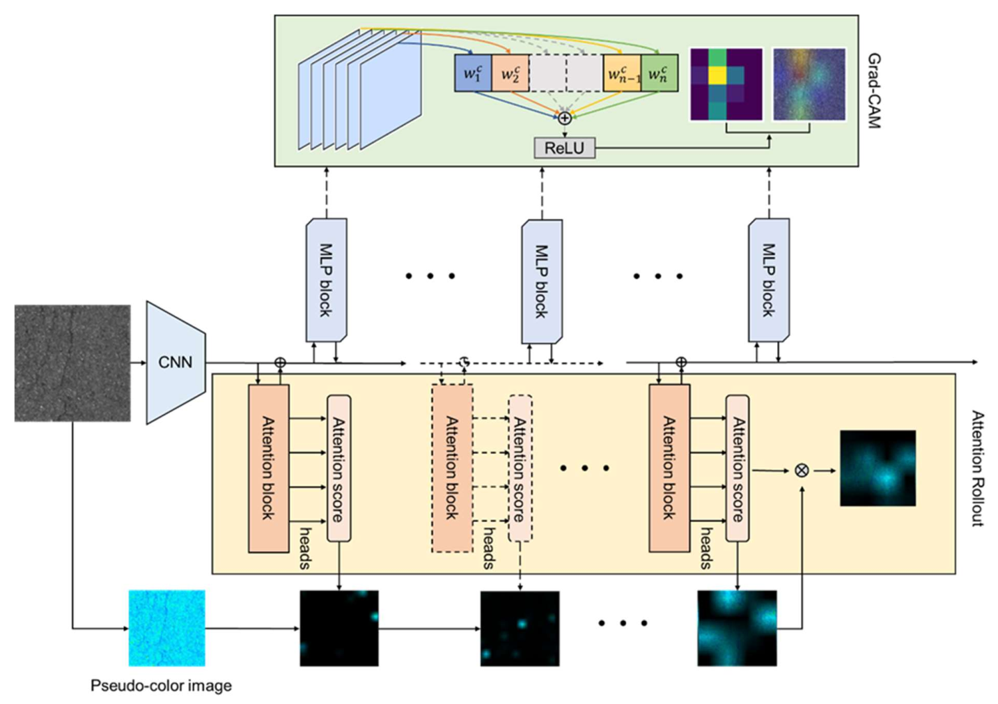
As the deep learning algorithms have been criticized as black boxes, this section will try to interpret the proposed models visually and help us better understand the proposed algorithms’ operation mode. Figure 9 shows the visual explanation methods used in this study. The visual interpretation of MLP blocks and the attention blocks are both explored.
For MLP layers, a technique called Gradient-weighted Class Activation Mapping (Grad-CAM) [33] was employed to explain what image features are learned at each network layer.
The gradient information in the specific convolutional layers was attained to assign an importance score for every neuron to acquire the class activation maps in Grad-CAM. Assume the output logits of a specific layer of class c is yc and the activation of feature map is Ak, the gradient of class c is calculated. Global average pooling is conducted in the gradient of width and height. Then the importance weight of neurons is attained as , shown in Equation (9) [33]:
where i and j represent the index of gradients in width and height. A represents the output feature map of this layer. k represents the channel of the feature map. is the gradients via back-propagation. Z is the total number of pixels in this feature map. is the function of global average pooling.
All the channels of feature maps are linear weighted and sum up to get the heat map, as shown in Equation (10) [33]. Only regions that have a positive effect on class c are reserved using the activation function ReLU, seen in Equation (11).
For attention layers, the attention maps of each attention lay were computed using the Attention Rollout [43]. It can be described as the following steps. First, the attention weights from each attention layer of LeViT were attained. Then, the attention weights across all heads of this layer were averaged. Next, recursively multiply the weight matrices of all layers, as seen in Equation (12). The attention from all positions in layer li to all positions in layer lj (j < i) is calculated:
where is attention rollout. A is raw attention. Matrix multiplication is conducted.
The original input images were transformed into pseudo-color images to highlight the attention mask applied to the input images. Finally, apply masks from the output token to the input space.
2.6. Evaluation Indexes
To evaluate the performance of the proposed model, the indices of accuracy, precision, recall rate, F1-score, and processing speed were calculated to evaluate the experimental results.
Accuracy (ACC) is the proportion of correctly classified samples in the total number of samples, seen in Equation (13):
where nc is the number of samples correctly predicted and nt is the total number of samples.
Precision (P) is the proportion of the samples predicted to be positive and is actually a positive sample (Equation (14)):
where TP is the positive samples that are correctly predicted and FP is the negative samples that are wrongly predicted to positive samples.
Recall (R) is the proportion of correctly predicted positive samples (Equation (15)):
where TN is the negative samples that are correctly predicted and FN is the negative samples that are wrongly predicted to positive cracks.
As P and R were unable to achieve high performance simultaneously, F1-score was used to take the harmonic mean of the two to measure the effectiveness of the model (Equation (16)):
As each class has equal weight, the Macro-Average principle is used when computing the evaluation metric. Metric within each category was calculated first, then the average resulting metrics across categories.
In addition, the computational costs were also evaluated for different methods. The number of the parameters, average training time per epoch, and inference time per step were set as the evaluation indexes.
3. Experimental Results and Analysis
3.1. Experimental Environment and Hyperparameters
The training software environment in this study was python 3.7, keras 2.3 with TensorFlow-2.5.0 backend. The operating system is Linux. All the experiments in this study were conducted in a supercomputing cluster equipped with a 7185 32C 2.0 GHz CPU with a 64-core Processor, 256 GB memory, and 8 DCU accelerator card.
A total of 100 training epochs were conducted with a batch size of 16 to improve the computation memory utilization. Adam [44] is the optimization algorithm for gradient descent in back-propagation in this study. The hyperparameters of the Adam algorithm were set as follows.
- (1)
- The learning rate was 1 × 10⁻⁴. The learning rate can control the weight update ratio and a lower learning rate allows the model to achieve better convergence.
- (2)
- β1 was 0.9 and β2 was 0.999. β1 and β2 can control the decay rates of the first and second moment means, respectively.
- (3)
- ε was 1 × 10⁻⁸, which prevented a relatively fixed value division by zero in the implementation.
Before training, the dataset was randomly shuffled before imputing into the networks. To reduce the training time, the transfer learning method was employed. The models were pretrained based on ImageNet [45], a large public dataset with approximately 15 million images.
3.2. Training Results of LeViT
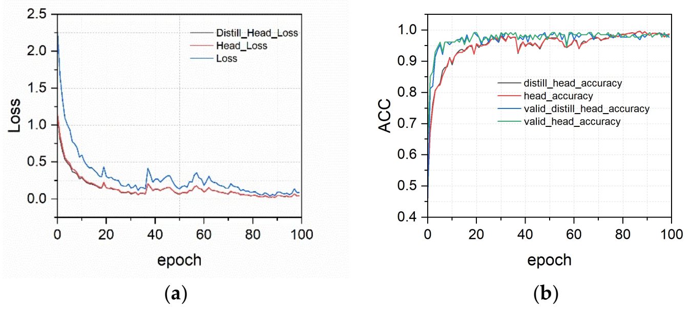
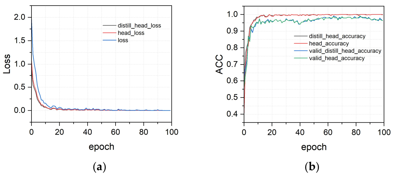
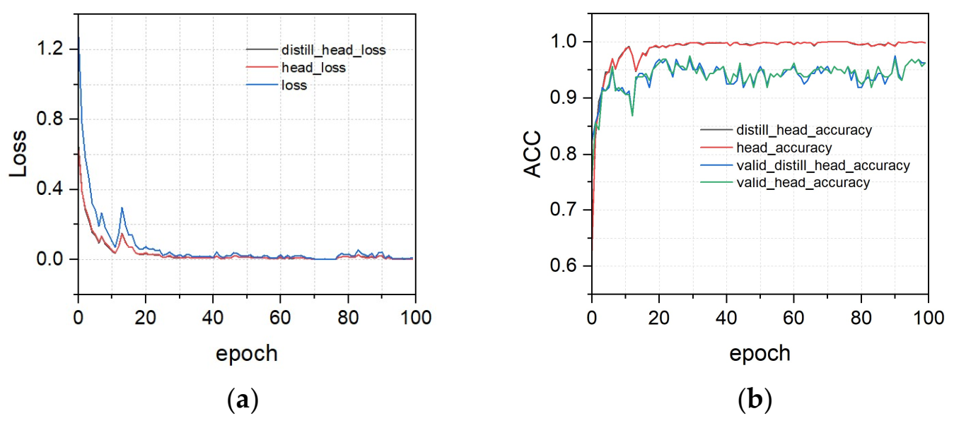
The training loss curves of two classification heads in the different datasets are presented in Figure 10a, Figure 11a and Figure 12a. During training, the supervised classifier and the distillation classifier work together, reaching convergence by the end of the training process. The training accuracy curves of the training and validation sets of different datasets based on LeViT are displayed in Figure 10b, Figure 11b and Figure 12b. The curves show that the training and validation loss drops rapidly at the beginning epochs and, after several epochs, they stabilize around a value with slight fluctuation.
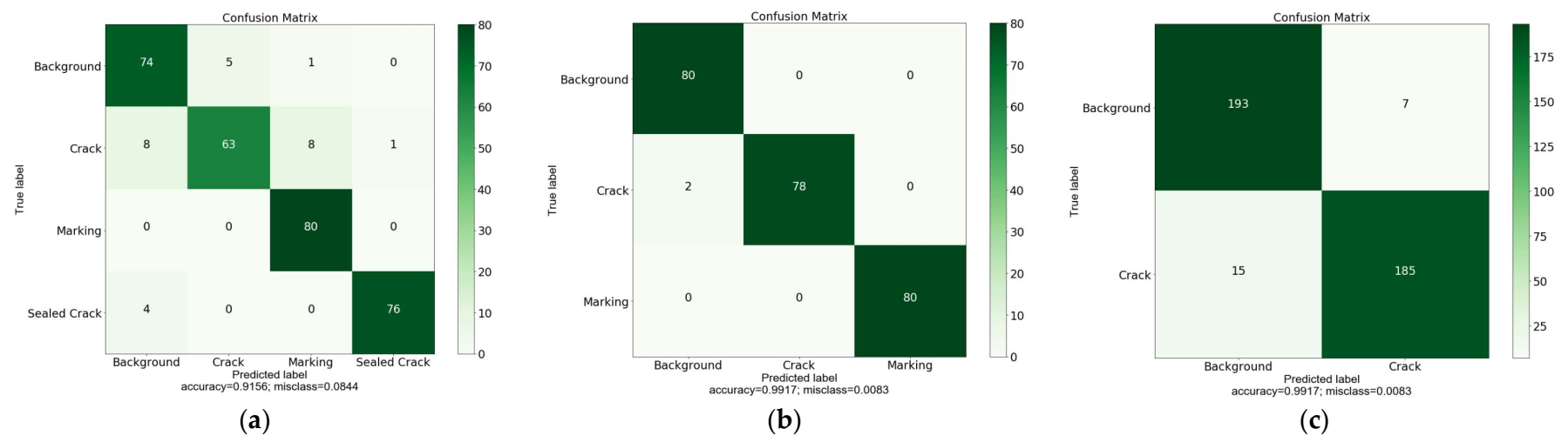
After 100 epochs of training, the LeViT model was tested by different test sets. Figure 13 shows the classification confusion matrix of different datasets. The overall classification accuracy of different test sets was 91.56%, 99.17%, and 94.50%, respectively. LeViT appears to have an excellent performance in classifying the images in dataset GAPs and Crack500. However, there are certain fusions of crack images. Among 80 crack images in the test set of JCAPs, eight images are misclassified as background, and eight images are misclassified as sealed crack images. The reason for these misclassifications could be the quality of the images. To obtain a better classification result, image augmentation methods can be used for further study.
3.3. Visual Interpretation
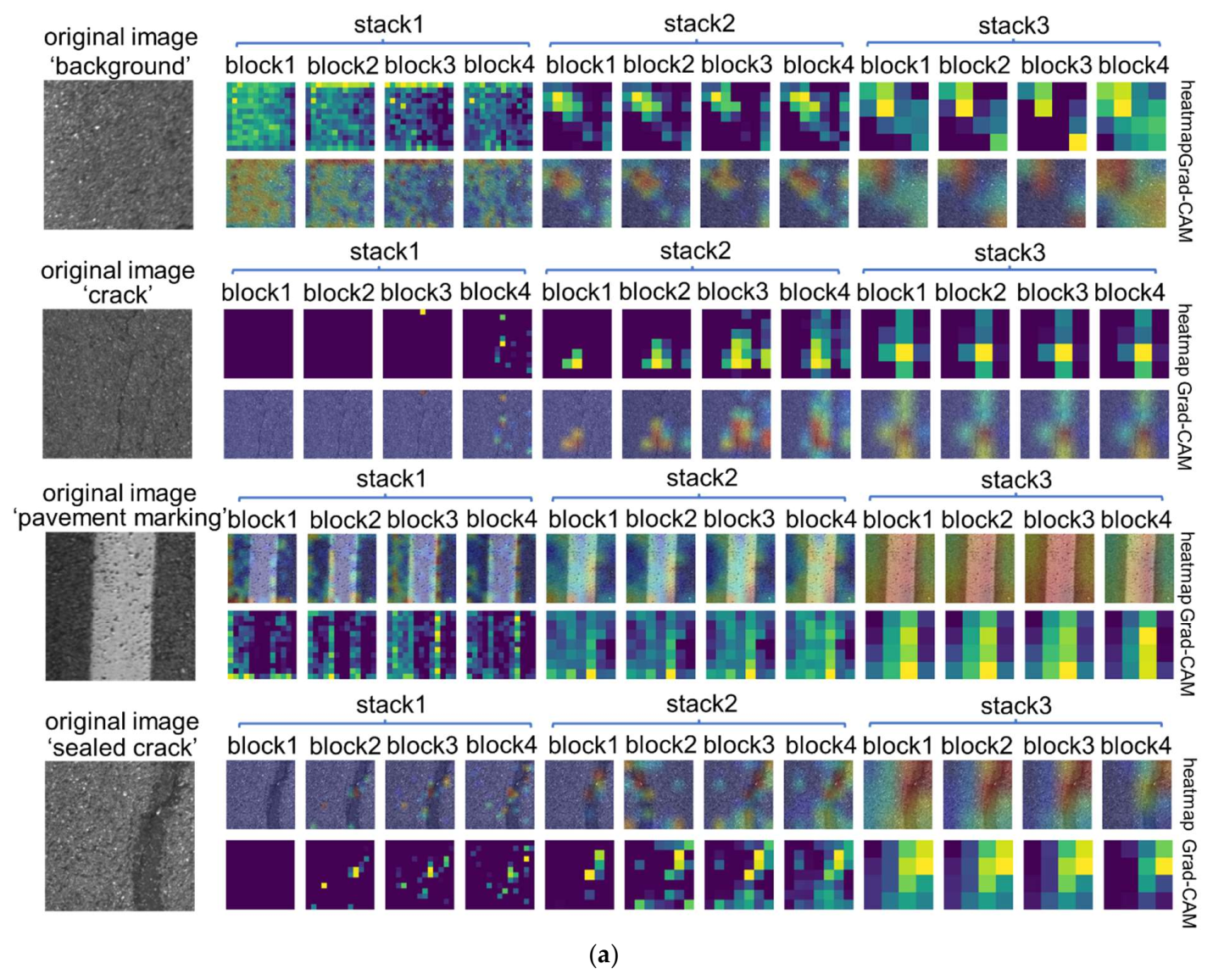
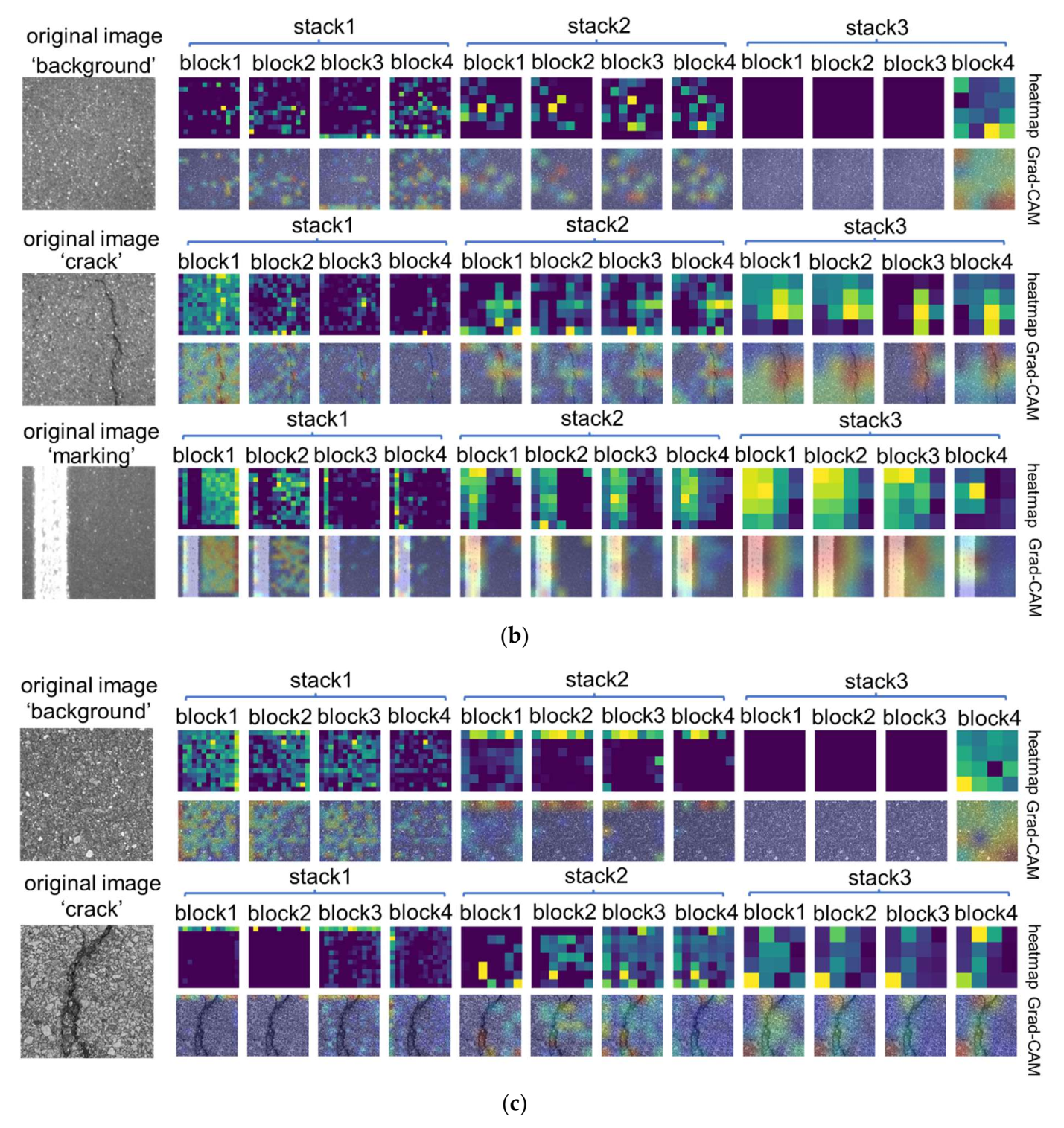
Visual interpretation results of both MLP blocs and attention blocks were explored. Figure 14 shows the visual explanation results of MLP blocks based on Grad-CAM. Figure 15 displays the interpretation results of attention blocks based on Attention Rollout.
The heat maps and Grad-CAM outputs from different MLP blocks of LeViT networks in different datasets are illustrated in Figure 14. In heat maps, the brighter color indicates regions that contribute more to the classification results in heat maps. Correspondingly in Grad-CAM output images, the red areas present higher scores for the class. As can be seen, for the ‘background’ class of the model, MLP blocks at the first stack have a wide range of focuses. In the following stack, blocks start to focus on some small regions. At the last stack, the blocks return to a broader focus and tend not to concentrate on small spots in the ‘background’ images. For the ‘crack’ and ‘sealed crack’ classes of the networks, as the layer of the LeViT network goes deeper, it generally learns to focus on the regions related to the specific objects and focus more on some small spots. As for the ‘pavement marking’, the blocks at the first stack concentrate mainly on the pavement background regions. In the following stacks, MLP blocks start to learn a more extensive range of area at the second stack. Finally, at the last stack, blocks gradually shift their attention to areas relevant to pavement marking and ignore the irrelevant regions. Overall, from the interpretation results, we can find that as the layer of the network goes deeper, it will focus more on the related part of the images. In addition, as can be seen in the heat maps of different classifications, the ‘crack’ and the ‘sealed crack’ have similar features with a long and wide light spot. To some extent, it explained why these two classifications of images were misclassified in the same class.
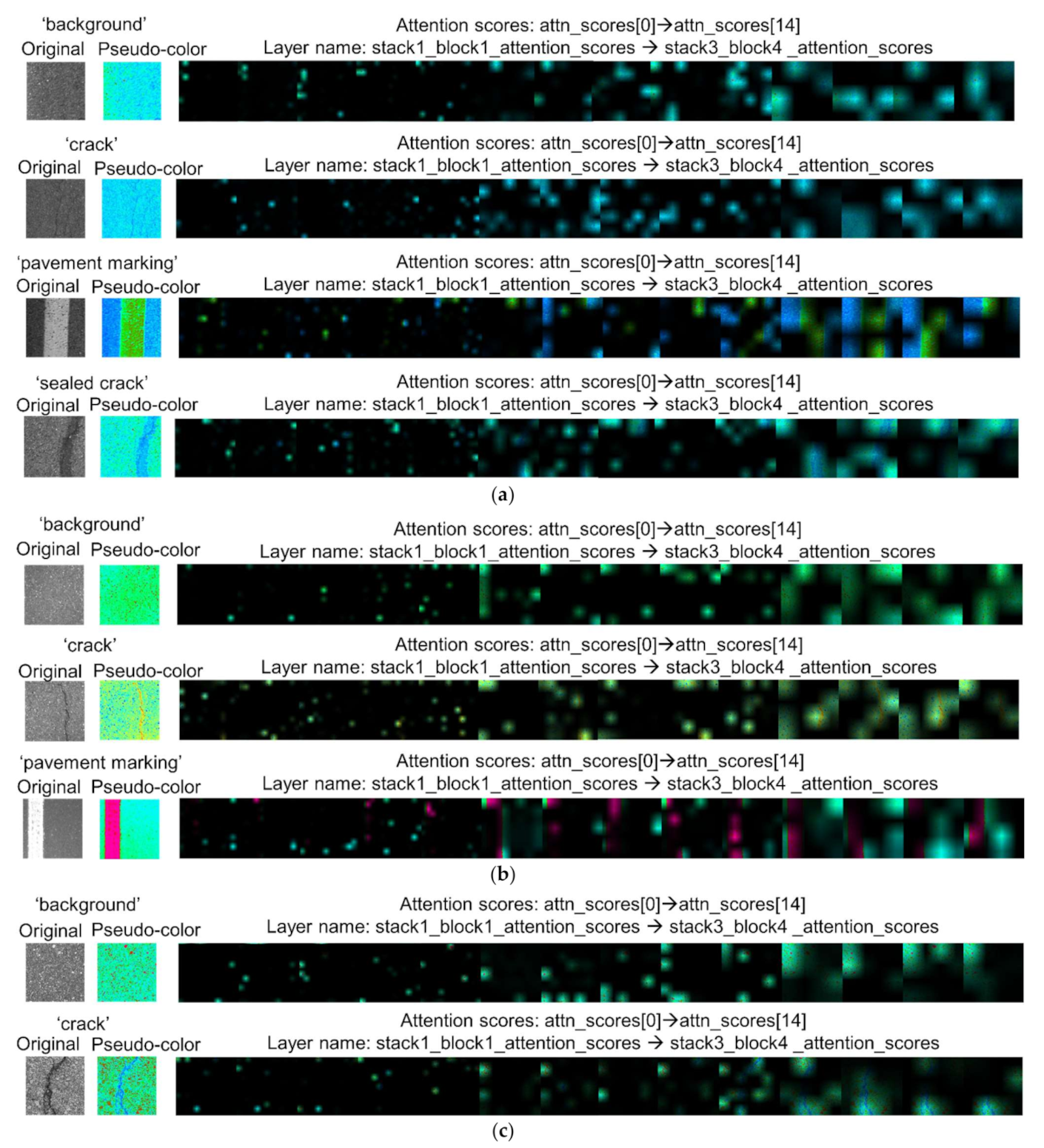
Figure 15 shows the attention score map from the output of different attention blocks. The regions with higher attention scores were highlighted by applying masks to areas with lower attention scores. From the visual interpretation results of the attention layers, in the first few attention blocks, the network pays almost equal attention to all regions in the images. Subsequently, in the following few regions, the network begins to focus on some separated and scattered regions in the images. As the layers get deeper, the regions of the posterior attention layers are connected to a larger area. Overall, there is a trend that the areas with higher attention scores will cover more effective feature areas in the deeper layers.
4. Discussion and Comparison
To validate the proposed methods, six popular models, including VGG-16 [7], ResNet-50 [9], InceptionV3 [46], DenseNet121 [10], MobileNetV1 [47], and ViT-b16 [24], were conducted for comparison. The basic principles of each method are as follows.
- VGG-16 [7]: This adopts a convolution kernel with a smaller size (3 × 3) and uses deeper layers to achieve good performance. VGG-16 means the number of its weight layer is 16.
- ResNet-50 [9]: The core idea of this network is its shortcut or skip connections. In residual blocks, the input information can detour to the output, which is helpful to decrease learning difficulties. ResNet-50 represents that the number of its weight layer is 50.
- InceptionNet-V3 [46]: Its main idea is to find out how to approximate the optimal locally sparse junction with dense components.
- Densenet-121 [10]: The core of the network is a dense block. The input to each layer of the network in the structure comes from the outputs of all the previous layers.
- MobileNet-V1 [47]: It is a lightweight network. A structure of depth-wise separable convolutions was introduced in this network.
Before training on our experimental dataset, pre-trained weights based on ImageNet of all the models were obtained to speed up the training process. During training, the hyperparameters were kept the same with LeViT, seen in Section 3.1. Sparse categorical cross-entropy was adopted to monitor the training process. The pre-trained weights of all the comparison models were obtained. The test results are provided in Table 3.
In the classification of dataset JCAPs, our model acquired the highest classification accuracy (91.56%), precision (91.72%), recall (91.56%), and F1-score (91.45%), while the original ViT network did not show competitive advantages compared with the equivalent CNN-based image classification model. Among all the classifications, the ‘crack’ images of our JCAPs dataset remain the biggest challenge for classification tasks.
In the test of dataset GAPs, our model also had the best performance with the highest classification accuracy (99.17%), precision (99.19%), recall (99.17%), and F1-score (99.17%). Among all the classifications, the ‘background’ images and the ‘pavement marking’ images reached the classification accuracy of 100.00%.
In the classification tasks of dataset Crack500, the accuracy, precision, recall, and F1-score of LeViT are 94.50%, 94.57%, 94.50%, and 94.50%, while the counterpart of the best-performed model is 95.00%, 95.11%, 95.00%, and 95.00%. The gap between them is acceptable.
Table 4 presents the comparison of training costs in dataset JCAPs. As the batch size is 16, the inference time per step is the processing time for every 16 images. From the table, it can be found that the proposed LeViT model has the fastest inference speed (86 ms/step) among all the comparison models. The average training time of LeViT for every epoch is 6.21 s, which is approximately 25% of the original ViT method and 80% of some prevailing CNN-based models, including DenseNet, VGG, and ResNet. Furthermore, the number of parameters in LeViT-192 is less than half of ResNet and InceptionNet, three-quarters of VGG, and one-eighth of original ViT. Although MobileNet has the fewest number of parameters among these methods, its inference speed is the lowest in our test. Overall, LeViT achieved competitive results with relatively fewer computation costs.
5. Conclusions
To solve the problem of high computation resources cost and poor interpretation of deep learning-based pavement image recognition models, this paper introduced a fast inference Transformer-based deep learning method called LeViT for the automatic object classification of pavement images. A visual explanation method was also employed to improve the interpretability of the proposed deep learning model. The performance of the proposed methods was evaluated on three different sources of pavement datasets. Compared to several state-of-the-art methods, LeViT attained the best classification accuracy, precision, recall, and F1-score in two pavement image datasets tested in this study. Moreover, the proposed LeViT model has a relatively faster inference speed (86 ms/step) among all the comparison models, which is approximately 80% of some prevailing CNN-based models, including DenseNet, VGG, and ResNet. Overall, the proposed method can achieve competitive performance with fewer computation costs. In addition, the proposed visual interpretation methods combining Grad-CAM and Attention Rollout can well visually explain the feature extraction mechanism of both MLP and attention blocks. Several issues that were not addressed in this study need to be noted. First, the impact of the number of the training images on the performance of the model was not be considered. Second, only longitudinal and transverse cracks are included in this research. For further study, more data containing alligator cracking can be added, and data augmentation methods can also be applied to improve the prediction performance of pavement images with poor quality.
Author Contributions
The authors confirm contributions to the paper as follows: study conception and design: Y.C. and X.G.; data collection: X.G. and J.L.; analysis and interpretation of results: Y.C. and Z.L.; draft manuscript preparation: Y.C., X.G., Z.L. and J.L. All authors have read and agreed to the published version of the manuscript.
Funding
This research received no external funding.
Institutional Review Board Statement
Not applicable.
Informed Consent Statement
Not applicable.
Data Availability Statement
Not applicable.
Conflicts of Interest
The authors declare no conflict of interest.
References
- Chen, C.; Chandra, S.; Han, Y.; Seo, H. Deep Learning-Based Thermal Image Analysis for Pavement Defect Detection and Classification Considering Complex Pavement Conditions. Remote Sens. 2021, 14, 106. [Google Scholar] [CrossRef]
- Liu, Z.; Wu, W.; Gu, X.; Li, S.; Wang, L.; Zhang, T. Application of combining YOLO models and 3D GPR images in road detection and maintenance. Remote Sens. 2021, 13, 1081. [Google Scholar] [CrossRef]
- Dorafshan, S.; Thomas, R.J.; Maguire, M. Comparison of deep convolutional neural networks and edge detectors for image-based crack detection in concrete. Constr. Build. Mater. 2018, 186, 1031–1045. [Google Scholar] [CrossRef]
- Hou, Y.; Li, Q.; Zhang, C.; Lu, G.; Ye, Z.; Chen, Y.; Wang, L.; Cao, D. The state-of-the-art review on applications of intrusive sensing, image processing techniques, and machine learning methods in pavement monitoring and analysis. Engineering 2021, 7, 845–856. [Google Scholar] [CrossRef]
- Liu, Z.; Gu, X.; Dong, Q.; Tu, S.; Li, S. 3D visualization of airport pavement quality based on BIM and WebGL integration. J. Transp. Eng. Part B Pavements 2021, 147, 04021024. [Google Scholar] [CrossRef]
- Krizhevsky, A.; Sutskever, I.; Hinton, G.E. Imagenet classification with deep convolutional neural networks. Adv. Neural Inf. Process. Syst. 2012, 25, 1097–1105. [Google Scholar] [CrossRef]
- Simonyan, K.; Zisserman, A. Very deep convolutional networks for large-scale image recognition. arXiv 2014, arXiv:1409.1556. [Google Scholar]
- He, K.; Zhang, X.; Ren, S.; Sun, J. Delving deep into rectifiers: Surpassing human-level performance on imagenet classification. In Proceedings of the IEEE International Conference on Computer Vision, Santiago, Chile, 7–13 December 2015; pp. 1026–1034. [Google Scholar]
- He, K.; Zhang, X.; Ren, S.; Sun, J. Deep residual learning for image recognition. In Proceedings of the IEEE Conference on Computer Vision and Pattern Recognition, Vegas, NV, USA, 27–30 June 2016; pp. 770–778. [Google Scholar]
- Huang, G.; Liu, Z.; Van Der Maaten, L.; Weinberger, K.Q. Densely connected convolutional networks. In Proceedings of the IEEE Conference on Computer Vision and Pattern Recognition, Honolulu, HI, USA, 21–26 July 2017; pp. 4700–4708. [Google Scholar]
- Zhang, A.; Wang, K.C.; Li, B.; Yang, E.; Dai, X.; Peng, Y.; Fei, Y.; Liu, Y.; Li, J.Q.; Chen, C. Automated pixel-level pavement crack detection on 3D asphalt surfaces using a deep-learning network. Comput.-Aided Civil Infrastruct. Eng. 2017, 32, 805–819. [Google Scholar] [CrossRef]
- Zhang, A.; Wang, K.C.; Fei, Y.; Liu, Y.; Tao, S.; Chen, C.; Li, J.Q.; Li, B. Deep learning–based fully automated pavement crack detection on 3D asphalt surfaces with an improved CrackNet. J. Comput. Civil. Eng. 2018, 32, 04018041. [Google Scholar] [CrossRef] [Green Version]
- Fei, Y.; Wang, K.C.; Zhang, A.; Chen, C.; Li, J.Q.; Liu, Y.; Yang, G.; Li, B. Pixel-level cracking detection on 3D asphalt pavement images through deep-learning-based CrackNet-V. IEEE Trans. Intell. Transp. Syst. 2019, 21, 273–284. [Google Scholar] [CrossRef]
- Hou, Y.; Li, Q.; Han, Q.; Peng, B.; Wang, L.; Gu, X.; Wang, D. MobileCrack: Object classification in asphalt pavements using an adaptive lightweight deep learning. J. Transp. Eng. Part B Pavements 2021, 147, 04020092. [Google Scholar] [CrossRef]
- Ali, L.; Alnajjar, F.; Jassmi, H.A.; Gochoo, M.; Khan, W.; Serhani, M.A. Performance Evaluation of Deep CNN-Based Crack Detection and Localization Techniques for Concrete Structures. Sensors 2021, 21, 1688. [Google Scholar] [CrossRef] [PubMed]
- Kim, B.; Yuvaraj, N.; Preethaa, K.S.; Pandian, R.A. Surface crack detection using deep learning with shallow CNN architecture for enhanced computation. Neural Comput. Appl. 2021, 33, 9289–9305. [Google Scholar] [CrossRef]
- Wu, Y.; Qi, S.; Sun, Y.; Xia, S.; Yao, Y.; Qian, W. A vision transformer for emphysema classification using CT images. Phys. Med. Biol. 2021, 66, 245016. [Google Scholar] [CrossRef]
- Liu, Z.; Chen, Y.; Gu, X.; Yeoh, J.K.; Zhang, Q. Visibility classification and influencing-factors analysis of airport: A deep learning approach. Atmos. Environ. 2022, 278, 119085. [Google Scholar] [CrossRef]
- Xingjian, S.; Chen, Z.; Wang, H.; Yeung, D.-Y.; Wong, W.-K.; Woo, W.-C. Convolutional LSTM network: A machine learning approach for precipitation nowcasting. In Proceedings of the Advances in Neural Information Processing Systems, Montreal, QC, Canada, 7–12 December 2015; pp. 802–810. [Google Scholar]
- Cho, K.; Van Merriënboer, B.; Gulcehre, C.; Bahdanau, D.; Bougares, F.; Schwenk, H.; Bengio, Y. Learning phrase representations using RNN encoder-decoder for statistical machine translation. arXiv 2014, arXiv:1406.1078. [Google Scholar]
- Zhang, A.; Wang, K.C.; Fei, Y.; Liu, Y.; Chen, C.; Yang, G.; Li, J.Q.; Yang, E.; Qiu, S. Automated pixel-level pavement crack detection on 3D asphalt surfaces with a recurrent neural network. Comput.-Aided Civil Infrastruct. Eng. 2019, 34, 213–229. [Google Scholar] [CrossRef]
- Vaswani, A.; Shazeer, N.; Parmar, N.; Uszkoreit, J.; Jones, L.; Gomez, A.N.; Kaiser, Ł.; Polosukhin, I. Attention is all you need. In Proceedings of the Advances in Neural Information Processing Systems, Long Beach, CA, USA, 4–9 December 2017; pp. 5998–6008. [Google Scholar]
- Bazi, Y.; Bashmal, L.; Rahhal, M.M.A.; Dayil, R.A.; Ajlan, N.A. Vision transformers for remote sensing image classification. Remote Sens. 2021, 13, 516. [Google Scholar] [CrossRef]
- Dosovitskiy, A.; Beyer, L.; Kolesnikov, A.; Weissenborn, D.; Zhai, X.; Unterthiner, T.; Dehghani, M.; Minderer, M.; Heigold, G.; Gelly, S. An image is worth 16x16 words: Transformers for image recognition at scale. arXiv 2020, arXiv:2010.11929. [Google Scholar]
- Zhou, D.; Kang, B.; Jin, X.; Yang, L.; Lian, X.; Jiang, Z.; Hou, Q.; Feng, J. Deepvit: Towards deeper vision transformer. arXiv 2021, arXiv:2103.11886. [Google Scholar]
- Touvron, H.; Cord, M.; Douze, M.; Massa, F.; Sablayrolles, A.; Jégou, H. Training data-efficient image transformers & distillation through attention. In Proceedings of the International Conference on Machine Learning, online, 18–24 July 2021; pp. 10347–10357. [Google Scholar]
- Chen, C.-F.; Fan, Q.; Panda, R. Crossvit: Cross-attention multi-scale vision transformer for image classification. arXiv 2021, arXiv:2103.14899. [Google Scholar]
- Mehta, S.; Rastegari, M. MobileViT: Light-weight, General-purpose, and Mobile-friendly Vision Transformer. arXiv 2021, arXiv:2110.02178. [Google Scholar]
- Liu, H.; Miao, X.; Mertz, C.; Xu, C.; Kong, H. CrackFormer: Transformer Network for Fine-Grained Crack Detection. In Proceedings of the IEEE/CVF International Conference on Computer Vision, Montreal, QC, Canada, 10–17 October 2021; pp. 3783–3792. [Google Scholar]
- Guo, J.-M.; Markoni, H. Transformer based Refinement Network for Accurate Crack Detection. In Proceedings of the 2021 International Conference on System Science and Engineering (ICSSE), Ho Chi Minh City, Vietnam, 26–28 August 2021; pp. 442–446. [Google Scholar]
- Graham, B.; El-Nouby, A.; Touvron, H.; Stock, P.; Joulin, A.; Jégou, H.; Douze, M. LeViT: A Vision Transformer in ConvNet’s Clothing for Faster Inference. arXiv 2021, arXiv:2104.01136. [Google Scholar]
- Castelvecchi, D. Can we open the black box of AI? Nat. News 2016, 538, 20–23. [Google Scholar] [CrossRef] [Green Version]
- Selvaraju, R.R.; Cogswell, M.; Das, A.; Vedantam, R.; Parikh, D.; Batra, D. Grad-cam: Visual explanations from deep networks via gradient-based localization. In Proceedings of the IEEE International Conference on Computer Vision, Venice, Italy, 22–29 October 2017; pp. 618–626. [Google Scholar]
- Serrano, S.; Smith, N.A. Is attention interpretable? arXiv 2019, arXiv:1906.03731. [Google Scholar]
- Eisenbach, M.; Stricker, R.; Seichter, D.; Amende, K.; Debes, K.; Sesselmann, M.; Ebersbach, D.; Stoeckert, U.; Gross, H.-M. How to get pavement distress detection ready for deep learning? A systematic approach. In Proceedings of the 2017 International Joint Conference on Neural Networks (IJCNN), Anchorage, AK, USA, 14–19 May 2017; pp. 2039–2047. [Google Scholar]
- Yang, F.; Zhang, L.; Yu, S.; Prokhorov, D.; Mei, X.; Ling, H. Feature pyramid and hierarchical boosting network for pavement crack detection. IEEE Trans. Intell. Transp. Syst. 2019, 21, 1525–1535. [Google Scholar] [CrossRef] [Green Version]
- Zhang, L.; Yang, F.; Zhang, Y.D.; Zhu, Y.J. Road crack detection using deep convolutional neural network. In Proceedings of the 2016 IEEE International Conference on Image Processing (ICIP), Phoenix, AZ, USA, 25–28 September 2016; pp. 3708–3712. [Google Scholar]
- Bahdanau, D.; Cho, K.; Bengio, Y. Neural machine translation by jointly learning to align and translate. arXiv 2014, arXiv:1409.0473. [Google Scholar]
- LeCun, Y.; Boser, B.; Denker, J.S.; Henderson, D.; Howard, R.E.; Hubbard, W.; Jackel, L.D. Backpropagation applied to handwritten zip code recognition. Neural Comput. 1989, 1, 541–551. [Google Scholar] [CrossRef]
- Ioffe, S.; Szegedy, C. Batch normalization: Accelerating deep network training by reducing internal covariate shift. In Proceedings of the International Conference on Machine Learning, Lile, France, 6–11 July 2015; pp. 448–456. [Google Scholar]
- Howard, A.; Sandler, M.; Chu, G.; Chen, L.-C.; Chen, B.; Tan, M.; Wang, W.; Zhu, Y.; Pang, R.; Vasudevan, V. Searching for mobilenetv3. In Proceedings of the IEEE/CVF International Conference on Computer Vision, Seol, Korea, 27–28 October 2019; pp. 1314–1324. [Google Scholar]
- Lin, M.; Chen, Q.; Yan, S. Network in network. arXiv 2013, arXiv:1312.4400. [Google Scholar]
- Abnar, S.; Zuidema, W. Quantifying attention flow in transformers. arXiv 2020, arXiv:2005.00928. [Google Scholar]
- Kingma, D.P.; Ba, J. Adam: A method for stochastic optimization. arXiv 2014, arXiv:1412.6980. [Google Scholar]
- Deng, J.; Dong, W.; Socher, R.; Li, L.-J.; Li, K.; Fei-Fei, L. Imagenet: A large-scale hierarchical image database. In Proceedings of the 2009 IEEE Conference on Computer Vision and Pattern Recognition, Miami, FL, USA, 20–25 June 2009; pp. 248–255. [Google Scholar]
- Szegedy, C.; Vanhoucke, V.; Ioffe, S.; Shlens, J.; Wojna, Z. Rethinking the inception architecture for computer vision. In Proceedings of the IEEE Conference on Computer Vision and Pattern Recognition, Las Vegas, NV, USA, 27–30 June 2016; pp. 2818–2826. [Google Scholar]
- Howard, A.G.; Zhu, M.; Chen, B.; Kalenichenko, D.; Wang, W.; Weyand, T.; Andreetto, M.; Adam, H. Mobilenets: Efficient convolutional neural networks for mobile vision applications. arXiv 2017, arXiv:1704. 04861. [Google Scholar]
Figure 1.
The framework of the proposed work.

Figure 2.
Example images from the JAPs dataset used in this study: (a) background, (b) crack, (c) pavement marking, and (d) sealed crack.
Figure 2.
Example images from the JAPs dataset used in this study: (a) background, (b) crack, (c) pavement marking, and (d) sealed crack.

Figure 3.
Example images from the GAPs dataset used in this study: (a) background, (b) crack, and (c) pavement marking.
Figure 3.
Example images from the GAPs dataset used in this study: (a) background, (b) crack, and (c) pavement marking.

Figure 4.
Example images from the Crack500 dataset used in this study: (a) background and (b) crack.
Figure 4.
Example images from the Crack500 dataset used in this study: (a) background and (b) crack.

Figure 5.
Structure of Vision Transformer (ViT).

Figure 7.
The architecture of the LeViT-192.

Figure 8.
The structure of multi-head attention in LeViT: (a) Regular attention block; (b) Attention block with subsampling function (shrink attention blocks). C is the channel of feature maps, and H and W represent the height and width, respectively, of the feature map. N is the number of self-attention heads. D is the output dimension of key K and query Q. Operator V has 2D channels.

Figure 9.
Visual interpretation methods used in this study.

Figure 10.
Training curves of JCAPs. (a) Loss curves of two classifier heads, (b) Training curves of training and validation set.
Figure 10.
Training curves of JCAPs. (a) Loss curves of two classifier heads, (b) Training curves of training and validation set.

Figure 11.
Training curves of GAPs. (a) Loss curves of two classifier heads, (b) Training curves of training and validation set.
Figure 11.
Training curves of GAPs. (a) Loss curves of two classifier heads, (b) Training curves of training and validation set.

Figure 12.
Training curves of Crack500. (a) Loss curves of two classifier heads, (b) Training curves of training and validation set.
Figure 12.
Training curves of Crack500. (a) Loss curves of two classifier heads, (b) Training curves of training and validation set.

Figure 13.
Confusion Matrix of LeViT in different test set: (a) JACPs, (b) GAPs, and (c) Crack500.

Figure 14.
The heat maps and Grad-CAM images of different classifications in different datasets. (a) JACPs, (b) GAPs, (c) Crack500.
Figure 14.
The heat maps and Grad-CAM images of different classifications in different datasets. (a) JACPs, (b) GAPs, (c) Crack500.


Figure 15.
The attention score maps of different classifications. (a) JCAPs, (b) GAPs, (c) Crack500.
Figure 15.
The attention score maps of different classifications. (a) JCAPs, (b) GAPs, (c) Crack500.


Table 1.
Distribution of different datasets used in this study.
| Datasets | Number of Images | Background | Crack | Pavement Marking | Sealed Crack | |
|---|---|---|---|---|---|---|
| JCAPs | Training set | 960 | 240 | 240 | 240 | 240 |
| Validation set | 320 | 80 | 80 | 80 | 80 | |
| Test set | 320 | 80 | 80 | 80 | 80 | |
| All | 1600 | 400 | 400 | 400 | 400 | |
| GAPs | Training set | 720 | 240 | 240 | 240 | - |
| Validation set | 240 | 80 | 80 | 80 | ||
| Test set | 240 | 80 | 80 | 80 | - | |
| All | 1200 | 400 | 400 | 400 | - | |
| Crack500 | Training set | 1200 | 600 | 600 | - | - |
| Validation set | 400 | 200 | 200 | - | ||
| Test set | 400 | 200 | 200 | - | - | |
| All | 2000 | 1000 | 1000 | - | - | |
Table 2.
Parameters of LeViT-192. Each stage contains pairs of attention and MLP blocks. C is the number of channels in MLP blocks. N is the number of heads in attention blocks. n is the number of the classifications.
Table 2.
Parameters of LeViT-192. Each stage contains pairs of attention and MLP blocks. C is the number of channels in MLP blocks. N is the number of heads in attention blocks. n is the number of the classifications.
| Layers | Operation | Output Size | |
|---|---|---|---|
| Convolutional layers | 4 × [Conv 3 × 3, stride = 2] | 14 × 14 × 192 | |
| Transformer stages | Stage 1 | 14 × 14 × 192 | |
| Subsample | , N = 6] | 7 × 7 × 288 | |
| Stage 2 | 7 × 7 × 288 | ||
| Subsample | . ] | 4 × 4 × 384 | |
| Stage 3 | 4 × 4 × 384 | ||
| Classification layers | Average Pooling | 384 | |
| Classifiers | [n, n] | ||
Table 3.
Classification results of different methods based on different datasets.
| Dataset | Method | All Classifications | Background | Crack | Pavement Marking | Sealed Crack | |||||||
|---|---|---|---|---|---|---|---|---|---|---|---|---|---|
| ACC (%) | P (%) | R (%) | F1 (%) | ACC (%) | F1 (%) | ACC (%) | F1 (%) | ACC (%) | F1 (%) | ACC (%) | F1 (%) | ||
| JCAPs | ViT | 88.13 | 89.33 | 88.13 | 88.21 | 83.75 | 88.16 | 77.50 | 82.67 | 93.75 | 96.77 | 97.50 | 85.25 |
| ResNet | 88.75 | 89.12 | 88.75 | 88.80 | 88.75 | 87.65 | 85.00 | 85.54 | 87.50 | 92.71 | 93.75 | 89.29 | |
| DenseNet | 88.75 | 89.55 | 88.75 | 88.61 | 97.50 | 96.30 | 70.00 | 79.43 | 97.50 | 96.89 | 90.00 | 81.81 | |
| VGG | 89.38 | 90.16 | 89.38 | 89.45 | 92.50 | 82.50 | 87.50 | 87.50 | 91.25 | 94.81 | 96.25 | 87.50 | |
| InceptionNet | 89.69 | 90.12 | 89.69 | 89.64 | 91.25 | 87.95 | 78.75 | 85.71 | 93.75 | 94.94 | 95.50 | 89.94 | |
| MobileNet | 90.31 | 91.03 | 90.31 | 90.35 | 96.25 | 91.12 | 82.50 | 82.50 | 88.75 | 94.04 | 93.75 | 88.24 | |
| Levit(ours) | 91.56 | 91.72 | 91.56 | 91.45 | 92.50 | 89.16 | 78.75 | 85.14 | 100.00 | 99.38 | 95.00 | 92.12 | |
| GAPs | InceptionNet | 97.08 | 97.15 | 97.08 | 97.10 | 96.25 | 96.86 | 97.50 | 95.71 | 97.50 | 98.73 | - | - |
| DenseNet | 98.33 | 98.38 | 98.33 | 98.32 | 100.00 | 98.16 | 95.00 | 97.44 | 100.00 | 99.38 | - | - | |
| ViT | 98.33 | 98.38 | 98.33 | 98.32 | 100.00 | 98.16 | 95.00 | 97.44 | 100.00 | 99.38 | - | - | |
| ResNet | 98.75 | 98.80 | 98.75 | 98.75 | 100.00 | 98.16 | 97.50 | 98.73 | 98.75 | 99.37 | - | - | |
| MobileNet | 98.75 | 98.80 | 98.75 | 98.75 | 100.00 | 98.16 | 96.25 | 98.09 | 100.00 | 100.00 | - | - | |
| VGG | 98.75 | 99.17 | 99.17 | 99.17 | 100.00 | 99.38 | 98.75 | 98.75 | 98.75 | 99.37 | - | - | |
| Levit(ours) | 99.17 | 99.19 | 99.17 | 99.17 | 100.00 | 100.00 | 97.50 | 98.73 | 100.00 | 100.00 | - | - | |
| Crack500 | InceptionNet | 92.00 | 92.60 | 92.00 | 91.97 | 98.00 | 92.45 | 86.00 | 91.49 | - | - | - | - |
| MobileNet | 93.75 | 93.88 | 93.75 | 93.75 | 96.50 | 93.92 | 91.00 | 93.57 | - | - | - | - | |
| VGG | 94.00 | 94.02 | 94.00 | 94.00 | 95.00 | 94.06 | 93.00 | 93.94 | - | - | - | - | |
| ViT | 94.00 | 94.07 | 94.00 | 94.00 | 96.00 | 94.12 | 92.00 | 93.88 | - | - | - | - | |
| LeViT(ours) | 94.50 | 94.57 | 94.50 | 94.50 | 96.50 | 94.61 | 92.50 | 94.39 | - | - | - | - | |
| ResNet | 94.75 | 95.08 | 94.75 | 94.74 | 99.00 | 94.96 | 90.50 | 94.52 | - | - | - | - | |
| DenseNet | 95.00 | 95.11 | 95.00 | 95.00 | 97.50 | 95.12 | 92.50 | 94.87 | - | - | - | - | |
Table 4.
Comparison of training costs in JCAPs.
| Method | Number of Parameters | Inference Time/Step | Average Training Time/Epoch |
|---|---|---|---|
| MobileNetV1 | 3.2 M | 3 s | 210.83 s |
| ViT-b16 | 85.8 M | 333 ms | 24.08 s |
| DenseNet-121 | 7.0 M | 103 ms | 7.45 s |
| VGG-16 | 14.7 M | 107 ms | 7.74 s |
| ResNet-50 | 23.6 M | 108 ms | 7.94 s |
| InceptionNetV3 | 21.8 M | 95 ms | 6.90 s |
| LeViT(ours) | 10.2 M | 86 ms | 6.21 s |
Publisher’s Note: MDPI stays neutral with regard to jurisdictional claims in published maps and institutional affiliations. |
© 2022 by the authors. Licensee MDPI, Basel, Switzerland. This article is an open access article distributed under the terms and conditions of the Creative Commons Attribution (CC BY) license (https://creativecommons.org/licenses/by/4.0/).
Share and Cite
MDPI and ACS Style
Chen, Y.; Gu, X.; Liu, Z.; Liang, J. A Fast Inference Vision Transformer for Automatic Pavement Image Classification and Its Visual Interpretation Method. Remote Sens. 2022, 14, 1877. https://doi.org/10.3390/rs14081877
AMA Style
Chen Y, Gu X, Liu Z, Liang J. A Fast Inference Vision Transformer for Automatic Pavement Image Classification and Its Visual Interpretation Method. Remote Sensing. 2022; 14(8):1877. https://doi.org/10.3390/rs14081877
Chicago/Turabian StyleChen, Yihan, Xingyu Gu, Zhen Liu, and Jia Liang. 2022. "A Fast Inference Vision Transformer for Automatic Pavement Image Classification and Its Visual Interpretation Method" Remote Sensing 14, no. 8: 1877. https://doi.org/10.3390/rs14081877
Note that from the first issue of 2016, this journal uses article numbers instead of page numbers. See further details here.