A Review of Remote Sensing for Water Quality Retrieval: Progress and Challenges

Abstract

Water pollution has become one of the most serious issues threatening water environments, water as a resource and human health. The most urgent and effective measures rely on dynamic and accurate water quality monitoring on a large scale. Due to their temporal and spatial advantages, remote sensing technologies have been widely used to retrieve water quality data. With the development of hyper-spectral sensors, unmanned aerial vehicles (UAV) and artificial intelligence, there has been significant advancement in remotely sensed water quality retrieval owing to various data availabilities and retrieval methodologies. This article presents the application of remote sensing for water quality retrieval, and mainly discusses the research progress in terms of data sources and retrieval modes. In particular, we summarize some retrieval algorithms for several specific water quality variables, including total suspended matter (TSM), chlorophyll-a (Chl–a), colored dissolved organic matter (CDOM), chemical oxygen demand (COD), total nitrogen (TN) and total phosphorus (TP). We also discuss the significant challenges to atmospheric correction, remotely sensed data resolution, and retrieval model applicability in the domains of spatial, temporal and water complexity. Finally, we propose possible solutions to these challenges. The review can provide detailed references for future development and research in water quality retrieval.

1. Introduction

According to the Global Risks Report 2020, the water crisis, including water shortage, water pollution and other water issues, is ranked fifth out of the the top 10 risks in terms of impact. In particular, water pollution has been becoming a complex and frustrating problem threatening many countries’ economy and technology policies [1]. Water pollution monitoring is an important basis for the comprehensive evaluation of water quality on both a regional and a national scale [2,3]. Therefore, accurate and fast water environment monitoring is especially important.

Traditionally, in situ measurements can obtain precise water quality parameters by using certain sampling points, but it is time-consuming, laborious and high costs with limits on large-scale monitoring [4,5]. Due to advantages of spatial and temporal coverage, remote sensing technology has been used to reflect the spatial distribution and dynamic changes in water quality components [6,7,8,9]. Owing to high frequency data acquisition and large-scale coverage, various spaceborne sensors with visible, infrared and microwave wavelengths can be used to monitor water quality. In the microwave domain, radiometers and synthetic aperture radars may be marginally helpful in the estimation of sea surface temperature and sea surface salinity [10], while in the VIS and IR domains, a range of spectral remotely sensed data have been proven successfully and widely used in water quality retrieval [11,12,13,14]. Data from Landsat-9, which launched in September 2021, are now publicly available to users and researchers around the world. Except for far-distance sensing platforms, the use of unmanned aerial vehicles (UAV) as a kind of prevailing airborne platform, provides good conditions for water quality retrieval because of their flexibility and portability for carrying multiple or high spectrum sensors [15,16].

The key of water quality retrieval is to dissect the relationship between the water constituents’ concentration and scattering signals (i.e., water-leaving radiance) from the sensors. The spectrum transfer process between water substances and sensors can be illustrated as it is shown in Figure 1 [17]. For different optical active components (OAC), the retrieval model can be established based on the relationship between inherent optical properties (IOP) and remote sensing reflection. IOP is an optical property of water that has nothing to do with external conditions and is only related to the composition of the water body. Additionally, then water quality parameters can be directly retrieved including Chl–a, SM, and CDOM [18,19,20]. Non-optically active substances in water have no direct optical characteristics, such as TN, TP, COD, dissolved oxygen (DO), etc., which can also be proceeded according to relationships between different substances in water or by using Artificial Intelligence (AI) [21,22]. However, to quantitively retrieve various water quality parameters, calculating the water-leaving reflectance is essential and complicated, because of the radiation at various wavelengths transferred among the atmosphere, water surface and water body. Generally, remote sensing-based water quality retrieval modes can be classified into four categories: empirical mode, physical mode, semi-empirical mode and intelligent mode. Among them, the AI mode is also a kind of empirical mode using different statistical approaches.

A large number of reviews presented many achievements in water quality remote sensing retrieval, mainly focusing on multi-source remotely sensed data and retrieval methods [23,24,25,26,27,28,29]. However, a comprehensive review will still provide an understanding of the state-of-the-art of water quality, especially under the urgent requirements for sustainable development. This paper summarizes a relatively thorough review of the current progress on optical remote sensing water quality retrieval in terms of data sources, retrieval modes and several specific water quality parameters retrieval algorithms. We still also indicate the significant challenges, including atmospheric correction, spatial and seasonal applicability of inversion models, and the mutual interference of the spectrum of water quality indicators. Finally, we propose possible solutions for the current challenges of remote sensing water quality retrieval.

2. Available Data Sources for Remote Sensing Water Quality Retrieval

2.1. Satellite-Borne Remote Sensing Data

2.1.1. Multispectral Data

Multispectral data, mostly with 3–10 bands, available for remote sensing water quality retrieval, includes MSS, TM, ETM+, OLI, ESA’s Sentinel-2, ENVISAT MERIS, France’s SPOT satellite data, and NOAA’s AVHRR data [30,31]. Recently, China’s GF series data and HJ data have also been used by some scholars [32,33]. Considering the spatial, temporal and spectral resolution and the accessibility, Landsat series data are the most commonly used for water quality monitoring, such as TSM, COD and TP [34,35]. Generally, due to resolution limitations, multi-spectral remote sensing water quality retrieval models are mainly constructed with empirical methods, which are more suitable for a certain specified period or water area.

2.1.2. Hyperspectral Data

Hyperspectral satellites have multiple bands with about 0.01 μm spectral resolution. Hyperspectral data, including the USA’s Hyperion data and HIS data of China’s HJ-1 satellite have been used for water quality retrieval [36]. Higher spectral resolution data have plentiful bands, which can be selected precisely and optimally for establishing water quality retrieval methods to distinguish the spectral mixing differences in multispectral data, thus greatly improving the accuracy of water quality parameters retrieval algorithms and showing good application potential [37,38,39].

2.2. Non-Satellite Remote Sensing Data

Non-satellite remote sensing data have been used in recent years, and various airborne remote sensing data and ground measured spectral data can also be used as data sources for remote sensing water quality retrieval. With the rapid progress of UAV technology, the light and small UAV system, equipped with multi-spectral camera, high spectrometer, infrared sensor and Lidar, is convenient and effective in water environment management [11,40]. For example, the USA’s AVIRIS with 220 channels and Canada’s Compact Airborne Spectrographic Imager (CASI) with 48 channels were extensively used for water environment monitoring. In addition, airborne Chinese Imaging spectrometer (CIS) data were also applied to monitor water environment. Nevertheless, airborne-based data have the limitations of high flight costs or uncertain risks. Except for the airborne-based spectrometer, portable spectrometers can be flexibly used on board to detect the water surface reflectance with adjustable spectral ranges. For example, the SVC HR-1024 portable field spec radiometer has 1024 bands with a range of 350~2500 nm [33]. Some portable spectrometers, including L1–1800, ASD Field Spec Pro and PSR-1100 are also popular within water quality management. Non-satellite spectrometers have the strength of having higher spectral and spatial resolution and they can provide continuous ground feature spectral curves. In addition, compared with satellite data, non-satellite remote sensing data are much less affected by the atmosphere. However, non-satellite remote sensing data sources based on aircraft measurement or ground measurement have a higher cost and are limited by their weak capacity for comprehensive observation of large areas of lakes and rivers. Some of the satellites available for water quality retrieval are presented in

Table 1. Available satellites for remote sensing water quality retrieval (bands more than 5).

	Satellite Sensor	Launch Date	Spatial Resolution (m)	Spectral Resolution Band	Temporal Resolution (Day)
Multi- spectral	NIMBUS-7 CZCS	1978.10	825	6	6
	Landsat-5/7/8/9	1984–2020	30	5	16
	SeaWiFS	1997.8	1130	8	16
	NOAA-16 AVHRR	2000.10	1100–4000	6	9
	EO-1 ALI	2000.11	10	9	16
	WorldView-2/3	2009/2014	1.85/1.24	8	1.1
	MERIS	2002.3	300–1200	15	1
	MODIS	1999.12	250–500–1000	9	0.5
	Landsat-8 OLI	2013.2	30	7	16
Hyper- spectral	HY-1A COCTS	2002.5	1100	10	3
	PROBA CHRIS	2001.10	18–36	19	7
	Hyperion	2000.11	30	42	16
	HJ-1A HSI	2008.9	100	128	4
	HICO	2009.9	100	128	10
	VIIRS	2011.10	375–750	22	0.5
	OHS	2018.4	10	32	2
	GF5-AHSI	2018.5	30	330	3
	ZY1-02D	2019.9	30	166	3
sensors for UAV	ZK-VNR-FPG480	/	0.09	270	/
	GaiaSky-mini	/	0.04	176	/

, which includes a wide spectral range. According to the research of Liu, although shortwave infrared (SWIR) and near infrared (NIR) are mainly used for turbid waters and clear waters individually, the combination of SWIR and NIR can improve the application [41].

3. Water Quality Parameters Retrieval Modes

3.1. Empirical Mode

The empirical mode (EM) is a kind of correlation statistical regression formula, which can be established by using a ground-measured water quality parameter value and reflectance of the optimal band or combination of bands [40]. The advantage of the empirical mode is that it is simple and easy to operate, and can be refined by selecting more precise spectral channels to increase the accuracy of water quality parameters retrieval [42]. However, the empirical mode has three obvious disadvantages. Firstly, it is hard for simple empirical models to meet the accuracy requirements of water quality parameters concentration estimation because the related spectral characteristics are mainly affected by the complex composition of water quality variables including phytoplankton pigments, SM, and CDOM, etc., which bring great uncertainty to the inversion of water quality concentration [23]. Secondly, due to regional and temporal constraints, empirical models have poor generalities and the established models in a certain water area may not be applicably used in other regions [43]. Finally, the empirical model requires a lot of field water quality sampling data as the basis to assure a relatively higher accuracy.

3.2. Analytical Mode

The analytical mode (AM) uses bio-optical models and radiation transmission models to simulate the propagation of light in the atmosphere and water bodies to describe the relationship between water quality components and the radiance or reflection spectrum of off-water radiation. In 1975, Gordon et al. proposed the general relationship between the apparent optical reflectance and water properties in water bodies [44]. This kind of quasi-single-scattering diffuse reflectance model represents an important foundation for the development of the analytical model as follows:

$$R_{rs}=f\left[\frac{b_b\left(\lambda \right)}{a\left(\lambda \right)+b_b\left(\lambda \right)}\right]$$

(1)

where $R_{rs}$ is the reflectance, $\lambda$ represents the wavelength,$a$ is the total absorption coefficient of water, $b_b$ is the total backscattering coefficient of water, and $f$ is the functional relation.

Based on the bio-optical inversion model, Gilerson calculated the Chl–a concentration of lakes in eastern Nebraska by using some sampling data [45]. However, the composition of the water body and radiation transmission procedure is rather complex because many factors need to be measured for the model to be established, such as the inherent optical characteristics of water, surface tourism characteristics, and water quality variables. In addition, the spectral resolution of most satellite sensors and those measured near the ground are inconsistent, which leads to some difficulties in model research. Therefore, the quantitative remote sensing inversion based on the analytical mode is difficult to achieve and is limited in practical applications [23,46].

3.3. Semi-Empirical Mode

The semi-empirical mode (SEM) is a combination of the empirical mode and the analytical mode. By using a certain paradigm derived from rigorous analytical models, SEM has a good applicability to calculate the water quality variables by combining only a small amount of in situ data and reflectance or radiance values. Some scholars used this method to retrieve water quality components such as SM, Chl–a, CDOM and associated visibility and turbidity with higher accuracies [47,48]. As for the study of suspended matter concentration retrieval, Lathrop [49], found that the SPOT–1 R band and Nir band were more sensitive to the suspended matter concentration, so they calculated different SM concentrations with R-G band ratio and Nir band based on the SEM mode. The semi-empirical method considers the optical characteristics of water quality parameters and has better portability than the empirical method.

3.4. Artificial Intelligence (AI) Mode

The Artificial Intelligence (AI) mode (AIM) is a kind of implicit algorithm that is different from above three modes (EM, AM and SEM) and that can provide explicit equations. Due to complicated and various background effects from the water surface, a combination of water quality parameters and sediment deposits, AIM mode can capture both linear and nonlinear relationships compared with traditional statistical or physical modes. A large number of scholars have applied the AIM mode such as neural networks (NN) and support vector machines (SVM) in water quality retrieval and achieved relatively satisfactory results [11,50]. The artificial neural network (ANN) model is a commonly used NN model. This method takes the gray value, radiance value or reflectance of each band of remote sensing data as the input of the NN model, and uses the water quality data as the output of the model. Generally, it is hard to accurately represent a simple linear relationship between water body component concentration and spectral reflectance or radiance. Therefore, the neural network method, as a nonlinear approximation method, is more flexible for water quality parameters retrieval. However, establishing a neural network for water quality retrieval requires a large number of samples to be trained with extensive experiences, otherwise there may be under-learning or over-learning situations, which greatly limit the neural network model inversion accuracy [51]. Compared with neural network models, SVM models can solve defects with small sample sizes. SVM uses nuclear functions to solve the computational complexity brought about by the dimensionality of high-dimensional space. SVM can solve the problem of convex optimization ensuring the global optimality of the algorithm. SVM is very suitable for solving the problems of small samples, nonlinearity, high dimensionality and local minimum points [52], but the increase in the number of training samples will make SVM algorithms difficult to implement and run slowly. In recent years, some scholars have applied the convolutional neural network model (Figure 2) to water quality parameters retrieval [12]. Yang proposed a Chl–a inversion model based on CNN with the matrix extension method to generate 5 × 5 grid pixel blocks, and the structure diagram of CNN and matrix expansion method was presented in Figure 3 [53]. The convolutional neural network has reduced the number of network parameters, alleviated the problem of overfitting, and accelerated the algorithm’s computing speed.

4. Progress in Water Quality Parameters Retrievals

4.1. Total Suspended Matter

Total suspended matter (TSM) concentration is one of the key parameters in main water quality components. The high concentration of SM in estuaries and inland lakes will disturb the optical properties of water, such as the depth of the true light layer, and then influence the growth of aquatic plants and the primary productivity of water bodies [54,55,56]. Researchers have developed some methods for estimating the concentration of TSM using remote sensing data, and have achieved good results in practical applications [57,58,59]. Table 2 shows a variety of SM inversion models. By studying the bio-optical model for turbid lakes with TSM concentrations within 5–50 g/m³, Dekker confirmed that the main values of the G and R bands (TM, HRV) are highly correlated with the TSM concentration with an exponential relationship (r² = 0.99) [60]. Based on Landsat data, Wang used a semi-empirical method to analyze the SM concentration changes in the Zhuhai estuary from 1987 to 2015, and indicated spatiotemporal changes in SM concentrations on the estuary coast [26]. Some scholars have used SPOT-6 data to calculate the SM concentration of narrow and diving rivers in mountainous areas through empirical methods, showing good results [61].

The reflectance in the 580–680 nm and 700–900 nm spectral range are most sensitive to TSM concentration changes, and are the best choice for TSM concentration remote sensing retrieval. Owing to above characteristic, Kallio used AISA imagery data to study the lakes in southern Finland, and designed the best algorithm for estimating TSM concentration with a single band reflectance of 705–714 nm [6]. In offshore water bodies, Miller used the statistical method and estimated the concentration of SM in the north Gulf of Mexico with channel-1 and channel-2 bands of MODIS data [62]. As for highly turbid waters (<985 g/m³) at the mouth of France’s Gerent, Doxaran disclosed that the increase in the concentration of SM had a strong relationship with the reflectivity ratio of 850 nm to 550 nm, and the results showed the potential of using the near infrared band to estimate the concentration of SM [63]. There are some TSM inversion models in Table 2, in which $C_{TSM}$ means the total suspended matter concentration, R (λ) means the remote sensing reflectance at wavelength λ, and MBP means a kind of matrix back propagation (MBP) neural network. The concentration range of TSM in the references is from 0.5 to 55 μg/L with an R² of above 0.65 and up to 0.89.

Table 2. Retrieval models of total suspended matter concentration (TSM).

Models	Modes	R2	Data	References
$\log \left(C_{TSM}\right)=a+b\ast \log R\left(710\right)$	EM	0.85	AISA	[6]
$C_{TSM}=-1.91\ast 1140.25R\left(645\right)$	EM	0.89	MODIS	[62]
$C_{TSM}=947.579{(R\left(660\right))}^{4.07}$	EM	0.65	SPOT6	[61]
$C_{TSM}=\frac{21428.77R\left(825\right)}{1-\frac{R\left(825\right)}{0.21}}-346.17$	EM	0.86	DEIMOS-1	[59]
$\log \left(C_{TSM}\right)=\frac{-b\pm \sqrt{b^2-4a\left(c-\frac{\log R\left(865\right)}{\log R\left(655\right)}\right)}}{2a}$	SEM	-	TM and OLI	[19]
$C_{TSM}=3.88{\left(R\left(645\right)\right)}^2+19.6R\left(645\right)$	SEM	0.79	In situ	[57]
Neural network (MBP)	IAM	0.72	MODIS	[58]

Table 2. Retrieval models of total suspended matter concentration (TSM).

Models	Modes	R2	Data	References
$\log \left(C_{TSM}\right)=a+b\ast \log R\left(710\right)$	EM	0.85	AISA	[6]
$C_{TSM}=-1.91\ast 1140.25R\left(645\right)$	EM	0.89	MODIS	[62]
$C_{TSM}=947.579{(R\left(660\right))}^{4.07}$	EM	0.65	SPOT6	[61]
$C_{TSM}=\frac{21428.77R\left(825\right)}{1-\frac{R\left(825\right)}{0.21}}-346.17$	EM	0.86	DEIMOS-1	[59]
$\log \left(C_{TSM}\right)=\frac{-b\pm \sqrt{b^2-4a\left(c-\frac{\log R\left(865\right)}{\log R\left(655\right)}\right)}}{2a}$	SEM	-	TM and OLI	[19]
$C_{TSM}=3.88{\left(R\left(645\right)\right)}^2+19.6R\left(645\right)$	SEM	0.79	In situ	[57]
Neural network (MBP)	IAM	0.72	MODIS	[58]

4.2. Chlorophyll–a

Chl–a can indicate the distribution of plankton biomass, and is the most basic indicator reflecting the primary productivity and eutrophication of water bodies. Various data sources, including hyperspectral data and multispectral data, have been well applied to the estimation of Chl–a concentration [6,12,64,65]. If the Chl–a concentration increases, the reflectance in the G and R bands increases, while the reflectance in the blue band decreases. Therefore, the selection of the optimal band depends on Chl–a [66]. When the concentration of Chl–a increased and the peak position moved from about 680 nm to around 715 nm with the increase in the peak amplitude value, Gitelson found that the reflection peak at 700 nm was important for the calculation of Chl–a concentration in inland waters [67]. Using the MERIS data from 2007 to 2012 in large turbid and complex shallow lakes, Palmer proposed a method for retrieving Chl–a concentration and temporal–spatial variations [25]. Boucher tested a variety of previously developed algorithms, covering 11 scenarios across 192 lakes, based on Landsat imagery from 2013 to 2015. The results suggest that remote sensing may be an effective and accessible regional-scale tool for monitoring programs of Chl–a in lakes [68]. We summarized four types of Chl–a concentration retrieving models.

(1)

Band ratio model

Chl–a content is usually retrieved with the reflectance of the maximum reflectance value in the Nir band and the minimum reflectance value in R. Kevin constructed a quantitative inversion model of Chl–a with negligible backscattering and incident light environment, which used a reflectivity ratio of 672 nm to 704 nm [69]. Using aerial hyperspectral data and MERIS imagery data, Sampas analyzed regression patterns through various possible channels or channel ratios to establish the best band ratio algorithm for Chl–a retrieval, and classified water quality indicators according to two classification criteria, in which Chl–a is divided into five levels with a classification accuracy of 78% [70].

(2)

First order differential model

The first order differential model, proposed by Rundquist [71], can remove the influence of partial noise spectra on the target spectrum. By using the differential model, the position of the spectral inflection point and the maximum and minimum reflectance wavelength can be determined. Luo concluded that under the condition of high Chl–a concentration, the wavelength position with the best effect of differential estimation of Chl–a concentration was 690 nm [72].

(3)

Three-band model

The three-band model generally uses three-band data to calculate the Chl–a content of water. This model was adaptable, to a certain extent, with high precision because the interaction of various water components can be eliminated partially with more bands used [73]. Subsequently, a semi-analytical three-band model for the inversion of Chl–a was developed in turbid water based on a bio-optical model [74]. Without any parameter adjustments, the MERIS data were used to verify the three-band model, and it was found that the simulated values of Chl–a were highly correlated with the measured values, which confirmed that the three-band Chl–a inversion model has a certain universality [75]. Using sampling data from lakes in eastern Nebraska, Gitelson proposed a Chl–a concentration estimation model based on the three-band algorithm explaining more than 89% of the Chl–a variation from 2 to 20 mg/m³ [76]. To better attenuate the effects of the absorption and backscattering of water quality, especially in the Nir band, Le improved the three-band model and introduced the fourth band model [77].

(4)

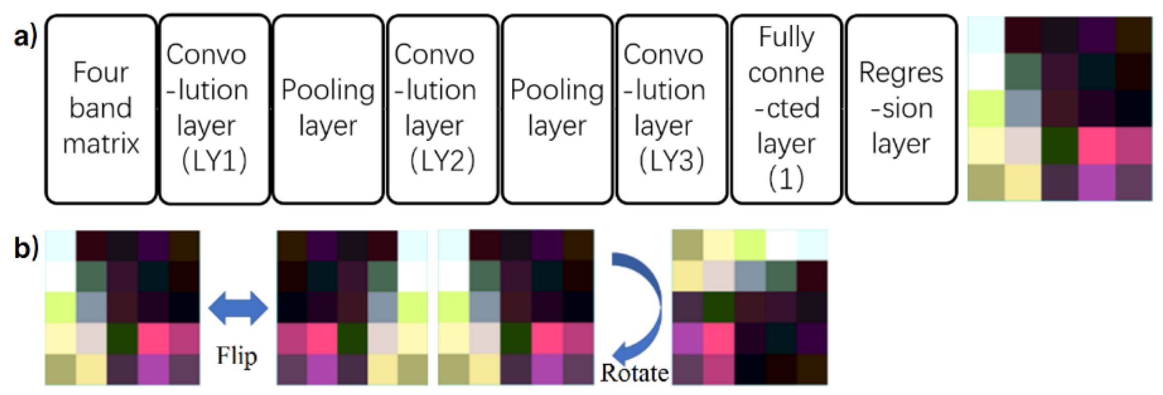
Artificial Intelligence model

By using remote sensing data, Zhang et al. [78] used an empirical neural network algorithm to calculate Chl–a content, and showed the results with a good accuracy. Singh established support vector machine regression model and classification model for Chl–a retrieval individually, and results disclosed the former model with a higher accuracy [52]. Song combined the measured spectral data and sampling data with a genetic algorithm to establish a Chl–a inversion model for four reservoirs in different regions, and found that neural network models were superior to three-band models in terms of spatial transferability [79]. Figure 4 shows the correlation curve of Chl–a inversion results based on convolutional neural network algorithm with good reliability (R² > 0.81) [53].

Some inversion models for Chl–a concentration are presented in

Table 3. Inversion models of Chl–a concentration.

Models	Modes	R2	Data	References
$C_{Chl-a}=\left(23.09\pm 0.98\right)+\left(117.42\pm 2.49\right)\ast \left[R^{-1}\left(665\right)-R\left(715\right)\right]\ast R\left(750\right)$ $C_{Chl-a}=-\left(16.2\pm 1.8\right)+\left(136.2\pm 3.2\right)\ast \left[R^{-1}\left(667\right)\ast R\left(748\right)\right]$	SEM	0.94 0.93	MERIS	[75]
$C_{Chl-a}=\frac{-b\pm \sqrt{b^2-4a\left[c-\left(R^{-1}\left(670\right)-R^{-1}\left(710\right)\right)\ast R\left(750\right)\right]}}{2a}$	SEM	0.89	MERIS	[76]
$C_{Chl-a}=\left[\left(R^{-1}\left(662\right)-R^{-1}\left(693\right)\right){\left(R^{-1}\left(740\right)-R^{-1}\left(705\right)\right)}^{-1}+b\right]/c$	SEM	0.97	In situ	[77]
$C_{Chl-a}=328.2\left(R^{-1}\left(656\right)-R^{-1}\left(716\right)\right)\ast R\left(753\right)+18.384$	SEM	0.84	HJ-1A HSI	[45]
$C_{Chl-a}=232.29\left[R^{-1}\left(665\right)-R^{-1}\left(708\right)\ast R\left(753\right)\right]+23.17$ $C_{Chl-a}=61.32R^{-1}\left(665\right)\ast R\left(708\right)-37.94$	EM	0.95 0.97	MERIS	[80]
Convolutional neural network	AIM	0.92	Airborne	[12]

. $C_{Chl-a}$ means the concentration or Chl–a, and R (λ) means the remote sensing reflectance at wavelength λ. Generally, empirical and semi-analytical algorithms are not only limited to the geographical applicability, but also to the accurate atmospheric correction which may cause uncertainties and difficulties. With the advances in Artificial Intelligence (AI) algorithms, AI models can meet this gap with their advantages of little requirement for prior knowledge. Some of inversion models for Chl–a are listed in Table 3, in which the concentration range of Chl–a in references is from 0 to 409 mg/m³ with an R² of 0.84 to 0.97.

4.3. Colored Dissolved Organic Matter

CDOM has a relatively complex composition, and it has an important impact on water color, underwater light field and chemical processes. CDOM can absorb part of ultraviolet and visible light. When the CDOM concentration increases, the absorption can extend to the blue band near 440 nm. Based on the measurement of the field and laboratory experimental data, Kowalczuk established a CDOM concentration inversion model in the Baltic Sea by using the remote sensing reflectance ratio ranging from 490 nm to 590 nm as independent variable [81]. In Mississippi River, Eurico and Richard proposed an empirical model and testified the best relationship between CDOM absorption (412 nm) and the reflectance ratios (510/555) with higher accuracy [82]. Using quasi-synchronous Advanced Land Imager (ALI) remote sensing data of two lakes in Finland and southern Sweden, Kutser analyzed CDOM absorption of filtrated water at 420 nm and developed CDOM retrieval algorithm using band 525–605 nm to band 630–690 nm [83]. Multiple remote sensing spectral reflectance ratios were testified to build a regression algorithm for retrieving yellow matter [84]. Based on the 412 nm and 555 nm bands of GOCI images, Moon et al. [85] established CDOM absorption coefficient α (440) inversion model. Duan analyzed the absorption coefficient and spectral slope of CDOM at 443 nm in different zones of Taihu Lake to disclose the black water blooms events [86]. Joshi et al. developed an empirical algorithm for CDOM retrieval from VIIRS images with the absorption coefficient at 412 nm (ag412) (Figure 5a), and there was a good performance in the validation of VIIRS ag412 against in situ observed ag412 (Figure 5b) [87]. In recent years, some studies have shown that Landsat-8 data can invert the CDOM absorption coefficient of inland water and this has achieved good results [88,89,90,91]. Some inversion models for CDOM concentrations are presented in

Table 4. Inversion models of CDOM Concentration.

Models	Modes	R2	Data	References
$C_{CDOM}\left(420\right)=5.13{\left(R\left(560\right)/R\left(660\right)\right)}^{-2.67}$	SEM	0.73	ALI	[83]
$C_{CDOM}\left(400\right)={10}^{(-0.2 - 0.5\log \left(R\left(490\right)/R\left(590\right)\right) + 0.65{(\log \left(R\left(490\right)/R\left(590\right)\right))}^2}$	EM	0.63	In situ	[81]
$C_{CDOM}\left(400\right)=0.2355{\left(R\left(412\right)/R\left(555\right)\right)}^{-1.3423}$	EM	0.85	GOCI	[85]
$C_{CDOM}\left(412\right)=3.18{\left(R\left(551\right)/R\left(671\right)\right)}^{-1.046}$	EM	0.87	VIIRS	[87]
$C_{CDOM}\left(400\right)=40.75e^{-2.463\left(R\left(563\right)/R\left(655\right)\right)}$	EM	0.83	OLI	[90]
Neural network (RBF)	IAM	0.972	USB2000+	[91]

. $C_{CDOM}$ means the concentration of CDOM, R (λ) means the remote sensing reflectance at wavelength λ, and MBP means a kind of matrix back propagation (MBP) neural network. In Table 4, the concentration range of CDOM in references is from 0.08 to 11.3/m with an R² from 0.63 to 0.97.

4.4. Chemical Oxygen Demand

The optical characteristics of COD in water bodies are not clear and are not suitable for using bio-optical models. Wang used the field-measured data and the Landsat TM satellite data to apply the empirical method to retrieve the COD of Shenzhen’s reservoir; the results confirm the feasibility of satellite image data estimating COD (R² = 0.791, p = 0.01) [92]. Based on the empirical model, Tao established an improved CODM index based on the combination of Landsat-8 OLI sensors B1, B7 and B4/B3, and quantitatively retrieved the concentration of CODM index in Taihu Lake (relative error 7.8%) [93]. Generally, the correlation of the COD concentration and remote sensing reflectance is a complex nonlinearity because of mutual interactions among water quality parameters. Din used a back-propagation network (BPMN) model and Support Vector Machine (SVM) model to retrieve COD (R² = 0.918) concentration based on Landsat-8 image data, and the results showed that the accuracy of the BPMN model was higher than that of the SVM model [94]. Some inversion models for COD concentrations are presented in

Table 5. Inversion models of COD Concentration.

Models	Modes	R2	Data	References
$$\begin{gathered} C_{COD}=2.76-17.27R\left(475\right)+72.15R\left(560\right) \\ -12.11R\left(660\right) \end{gathered}$$	EM	0.79	TM	[92]
$C_{COD}=e^{\left(0.367+1.2454\ln \left(R\left(560\right)/R\left(660\right)\right)\right)}$	EM	0.66	TM	[94]
Neural network	IAM	0.92	OLI	[22]

.$C_{COD}$ means the total suspended matter concentration, R (λ) means the remote sensing reflectance at wavelength λ. In Table 5, the concentration range of COD in references is from 1.6 to 4.8 mg/L with an R² from 0.66 to 0.92.

4.5. TP and TN Concentrations

TP and TN, as two important factors, has been widely studied to reflect the eutrophication of rivers and lakes, which has become a serious water pollution problem, deteriorating functions and threatening water security in many countries [95,96,97,98,99,100,101]. However, because the spectral response mechanism is not clear enough, there are still challenges to retrieving TN and TP by using remote sensing [43]. Based on Landsat TM data, Wu used statistical methods to establish a TP inversion model of the Qiantang River [102]. By using Landsat’s ETM + data and in situ data, Isenstein established a multivariate linear regression model to better disclose the nutrient distribution of Lake Champlain [103]. Based on the ratio method, Xu et al. [104] established the best regression model for retrieving TN and TP with a higher R² (0.839 and 0.934). Chang et al. [105] used a genetic algorithm to analyze the spatial distribution of TP based on MODIS image data in Tampa Bay, western Florida. Chebud et al. [50] used the neural network method to analyze TP distribution in the Kissimmee River basin. Some inversion models for TP and TN are presented in

Table 6. Inversion models of TP and TN.

Models	Modes	R2	Data	References
$C_{TP}=0.896+5.419x_1-3.016x_2$, $$\begin{gathered} \mathrm{Where},x_1=(\left(R\left(830\right)/R\left(475\right)- \\ \left(R\left(830\right)-R\left(475\right)\right)/\left(R\left(830\right)+R\left(475\right)\right)\right)/-ln\left(R\left(830\right)+R\left(560\right)\right) \\ x_2=(\left(R\left(830\right)/R\left(475\right)-\left(R\left(830\right)-R\left(475\right)\right)/\left(R\left(830\right)+R\left(475\right)\right)\right) \end{gathered}$$	EM	0.99	HJ-1A CCD	[43]
$C_{TN}=e^{15.39-0.92\left(R\left(555\right)+R\left(830\right)\right)/\ln \left(R\left(660\right)+R\left(830\right)\right)}/100$	EM	0.92	CBERS-1 CCD	[106]
$\ln \left(C_{TP}\right)=-21.45\left(\frac{R\left(660\right)}{R\left(560\right)}\right)-14.42\left(\frac{R\left(485\right)}{R\left(660\right)}\right)+42.99R\left(485\right)+27.1$	EM	0.77	TM	[102]
$C_{TN}=-22825.891R\left(455\right)+0.607\left(1015\right)/R\left(528\right)+4.659$	EM	0.78	In situ	[104]
$C_{TN}=0.116+2.071(R\left(655\right)/{\left(R\left(562+R\left(865\right)\right)\right)}^{1.26477}$ $C_{TP}=-0.2+0.005e^{\left(R\left(443\right)+R\left(562\right)+R\left(655\right)\right)/R\left(583\right)}$	EM	0.84; 0.8	OLI	[42]
$\mathrm{Neural}\mathrm{network}(C_{TP}$)	IAM	0.95	TM	[50]
$\mathrm{Genetic}\mathrm{programming}(C_{TP}$)	IAM	0.58	MODIS	[105]

.$C_{TP}$ and $C_{TN}$ mean the concentration or TP and TN, respectively, R (λ) means the remote sensing reflectance at wavelength λ. In Table 6, the concentration range of TP/TN in references is from 0.02 to 0.96 mg/L and 0.18 to 1.78 mg/L with an R² of 0.58 to 0.99 and 0.78 to 0.92 individually.

5. Challenges and Possible Solutions in Water Quality Retrievals

5.1. Atmospheric Correction

(1)

Challenges

In the process of water quality retrieval, the water-leaving radiance received by a sensor at the top of the atmosphere is not only dominated by water component parameters and water bottom absorbance, but is also significantly influenced by atmospheric scattering [107,108,109,110,111,112]. Due to aerosol scattering in the atmosphere, 80–90% of the signal collected by the sensor, within a majority of spectral ranges of ocean remote sensing, is light scattered by atmospheric molecules [113,114]. Water-leaving radiance, the most useful information for retrieving water quality, is seriously attenuated because of atmospheric influences. To solve this problem, atmospheric correction is crucial in order to eliminate the radiation error caused by the atmospheric influence so that more accurate results can be retrieved. Atmospheric models such as 6S, MODTRAN, spatially adaptive fast atmospheric correction (ATCOR), etc. are widely used for atmospheric correction [115,116,117].

However, some atmospheric parameters in many algorithms are pre-defined with average values or a certain atmospheric profile status, which cannot reflect the spatial and temporal variations. In addition, atmospheric correction algorithms bring about significant challenges because of their weak adaptability and high uncertainties. Warren et al. (2019) pointed out that there was room to improve the performance six atmospheric algorithms, including C2RCC v1.0, Polymer v4.6, Sen2Cor v2.4.0, Acolite v20170718, iCOR v1.0 and l2gen version 7.5.1 [118]. Accurate atmospheric correction models are a major part of water quality parameters inversion.

(2)

Possible solutions

Because the atmospheric correction model in the inland water environment is difficult, it is necessary to establish high precision atmospheric correction algorithms to improve the monitoring accuracy of water quality [119]. To overcome the adjacency effects caused by dark waters and bright land in NIR bands, a sensor-generic adjacency pre-processing method was proposed to enhance the precision of water quality parameters retrieval [120]. Combining different bands from different remote sensing data by using merging algorithms has proven to be feasible [121].

In addition to the remote sensing satellite data, UAV platforms with high-resolution sensors are capable of retrieving water quality without considering the influence from the atmosphere [122]. Therefore, researchers should focus on the relationship between satellite imagery and UAV image reflectance to establish a universal atmospheric correction model.

5.2. Remotely Sensed Data Resolution

(1)

Challenges

Most satellite data, such as MODIS, MERIS, GOCI, etc. are suitable for ocean color remote sensing water quality retrieval [123]. However, for inland water, especially for small lakes or narrow rivers, there are significant challenges in obtaining remotely sensed data with fine spectral, spatial and temporal resolution simultaneously. Due to the impact of the image signal-to-noise ratio, data storage and transmission, homogeneous remote sensing images are mutually restricted in terms of temporal, space and spectral resolutions [124,125]. Some remotely sensed data with high spatial resolution could not provide long series and dynamic monitoring because of low temporal resolution, while some data with high temporal resolution could not support detailed investigation because of coarser spatial resolution [126]. Except for the limitations in spatial and temporal resolution, high spectral resolution data are essential for remote sensing water quality retrieval. Although many hyper-spectral data, such as OLCI, HJ-1A HIS, HICO, VIIRS, etc., have continuous spectral bands to reflect water quality components, some of them cannot meet the requirements of finer spatial resolution [127]. In addition, weather conditions have a great impact on remote sensing images which are notably contaminated by clouds and fog in monsoon season.

(2)

Possible solutions

Recently, many data fusion methods have been proposed to generate high spatiotemporal resolution data by using Landsat and MODIS data, including the spatial and temporal adaptive reflectance fusion model (STARFM), spatiotemporal integrated temperature fusion model (STITFM) and flexible spatiotemporal data fusion method (FSDAF) [128,129], satisfying the need of long-term and fine-scale regional study. The spatial and temporal fusion of remote sensing images is a combination of high spatial resolution and high temporal resolution of multi-source remote sensing satellite data. Using the spatio-temporal fusion algorithm can generate image sequences with high spatio-temporal resolution in the target area [130,131]. The spatio-temporal fusion algorithm of remote sensing images integrates the advantages of multi-source data to meet the requirements of spatial and temporal resolution of water quality monitoring, especially for small lakes and rivers [132].

The requirement for generating high spatial, temporal and spectral resolution data is urgent. The spatio-temporal–spectral fusion method was proposed to generate high spatial, temporal and spectral data by using the combination of multi-source remote sensing. It can integrate the spatial, high-temporal, and hyper-spectral advantages of multi-source data to generate high-spatial, high-temporal, hyper-spectral images of the target area [133]. Figure 6 shows the framework of Workflow of the Hybrid Spatio-Temporal–Spectral image Fusion Model [134].

5.3. Retrieval Model Applicability

(1)

Challenges

Spatially, remote sensing water quality models are generally established for certain regional water bodies based on the relationship between spectral reflectance and in situ water quality parameters, representing the local water pollution, sky background and weather conditions. Because of this spatial dependency, these water quality retrieval models show a good performance in some regions but may be not applicable for other regions, especially using bio-optical models in which the regional IOPs plays the fundamental roles [135]. Huang established different COD retrieval models for three rivers in Qingyang city with Landsat TM data, and results showed the application of the limitations of empirical models in different regions [136].

Temporally, satellite-based water quality models are limited in temporal applicability because most models are designed by using in situ data collected in the short term. Due to meteorological variation, water quality components in the same water area varied in different seasons [137]. For example, a difference in water temperature may affect Chl–a due to dissolved oxygen variations in complex ways [28]. Michael pointed out that remote sensing water quality retrieval algorithms caused errors because of time periods and locations where the model optical parameters were different than the actual properties [138].

Spectral interaction is also one of the key challenges affecting the model applicability, especially in inland waters (less than case 2) with complex compositions [139]. Because of the influence of optically active constituents, it can cause the disturbance of mixture inherent optical properties (IOP) which make it difficult to distinguish different water quality components contributions from the total spectral water-leaving radiances [140]. Generally, one algorithm cannot obtain accurate water quality retrieval in the complex waters due to the interacted optical signals of different water quality components [141].

(2)

Possible solutions

Because of the complexity of water quality components’ interaction and spatiotemporal variation, solutions for improving retrieval model applicability may focus on the differences in water types, new methods and new data.

Previously, eight optical water types (OWT) was defined by their optical properties in the global ocean to characterize the uncertainties of water quality retrieval model [142]. Additionally, then OWT was extended to a blending approach for retrieving chlorophyll–a concentration in inland lakes [143]. Moreover, a typology of OWTs was developed with extensive representability by using various aquatic systems and conditions [144].

A regional generalized additive model (GAM)-based satellite Chl–a algorithm was evaluated and compared with OC3M Chl–a, and results showed that the GAM Chl–a improved accuracy in both magnitude and seasonality [145]. Machine learning-based models, with environmental variables dependence, can reflect complicated nonlinear relationships, and can be trained to improve their applicability [146,147]. Some environmental variables such water surface temperature (WST) can be obtained based on MODIS land surface temperature (LST) products MOD11L2, which was generated with MODIS bands 31 (11 μm) and 32 (12 μm) using a split-window algorithm [148]. Various methods are put forward with those advantages in different dimensions. Finding ways to effectively combine these methods is the key solution to enhancing the models’ applicability. For example, 19 models including empirical methods, peak height methods, neural networks and semi-analytical methods were calibrated to an ensemble, and then optimal models based on the OWT framework were assured of the Chl–a retrieval applicability in space and time dynamically [149].

With the technologies of sensing and platforms, airborne data have high spectra with powerful discrimination ability, which is helpful for retrieving inactive water quality parameters. There is a correlation between some non-optically active substances and optically active substances, such as nitrogen and phosphorus content [150]. As for long-term water quality monitoring, multisensory satellites data must be calibrated, validated and corrected with plentiful in situ measurements [151]. To develop in situ multi-sensor-system monitoring, within the international research project “Dynamics of Water Quality” (DYNAQUA) which aims to assure good water quality in the lake Taihu, depth- and time-resolved water quality profiles were frequently obtained with meteorological data and sampling data [152]. A combination of both satellite and airborne remote sensing is useful in assessing the quality of inland waters [153].

6. Conclusions

This paper summarizes the progress of remote sensing water quality retrieval including data sources, algorithm modes and some water quality parameters retrieval models, and indicates the current challenges and possible solutions.

(1)

A series of remotely sensed data including multispectral and hyperspectral data are widely used in water quality monitoring. With the rapid development of UAV performance, various airborne-based spectrometers can provide flexible and efficient solutions satisfying water quality retrieval with higher temporal, spatial and spectral resolution.

(2)

Four categories of retrieval modes including empirical mode, analytical mode, semi-empirical method, and intelligent algorithm mode are presented. The empirical method avoids the complex physical parameters and quickly establishes the inversion model of water quality parameters through simple regression analysis; however, the empirical method lacks the physical mechanism, and therefore the result is a great deal of uncertainty, and it has very poor portability in space and time. The semi-empirical method combines the reflectivity of water body with the concentration of measured parameters, which has a certain physical significance and is simple to apply, but the semi-empirical method relies on a large number of on-site measured data, and the time and spatial applicability is poor. The physical mechanism of the analytical method is clear, the calculation does not require many field samplings points, and the portability is strong; however, the analytical method requires high accuracy of the measuring instrument, the application cost is high, and it is not easy to popularize.

(3)

Models for estimating SM, Chl–a, CDOM, COD, TN and TP are thoroughly summarized. Because the optical properties of these substances are clear, the inversion method is gradually developed from empirical methods to theoretical methods. The emergence of more and more new terrestrial satellites has promoted the expansion of water quality remote sensing monitoring from the ocean to inland water bodies, and with the rapid development of machine learning algorithms, more new Artificial Intelligence (AI) is used in remote sensing inversion of non-optical active substances such as COD, TN and TP.

(4)

We also conducted a bibliometric analysis of the relevant literature in the field, analyzing relevant authors, organizations, and literature.

(5)

Three challenges and possible solutions were indicated for future research. The effects of remote sensing monitoring on water quality are explained from the aspects of the limitations of sensor performance, the complexity of atmospheric correction, the spatiotemporal variability of water optical characteristics, and the interaction between various water quality parameters and the possible solutions are put forward for future research studies.

References

- Han, D.; Currell, M.J.; Cao, G. Deep challenges for China’s war on water pollution. Environ. Pollut. 2016, 218, 1222–1233. [Google Scholar] [CrossRef] [Green Version]
- Moss, B. Cogs in the endless machine: Lakes, climate change and nutrient cycles: A review. Sci. Total Environ. 2012, 434, 130–142. [Google Scholar] [CrossRef]
- Swain, R.; Sahoo, B. Improving river water quality monitoring using satellite data products and a genetic algorithm processing approach. Sustain. Water Qual. Ecol. 2017, 9–10, 88–114. [Google Scholar] [CrossRef]
- Schaeffer, B.A.; Schaeffer, K.G.; Keith, D.; Lunetta, R.S.; Conmy, R.; Gould, R.W. Barriers to adopting satellite remote sensing for water quality management. Int. J. Remote Sens. 2013, 34, 7534–7544. [Google Scholar] [CrossRef]
- Brivio, P.A.; Giardino, C.; Zilioli, E. Validation of satellite data for quality assurance in lake monitoring applications. Sci. Total Environ. 2001, 268, 3–18. [Google Scholar] [CrossRef]
- Kallio, K.; Kutser, T.; Hannonen, T.; Koponen, S.; Pulliainen, J.; Vepsäläinen, J.; Pyhälahti, T. Retrieval of water quality from airborne imaging spectrometry of various lake types in different seasons. Sci. Total Environ. 2001, 268, 59–77. [Google Scholar] [CrossRef]
- Song, K.; Wang, Z.; Blackwell, J.; Zhang, B.; Li, F.; Jiang, G. Water quality monitoring using Landsat Themate Mapper data with empirical algorithms in Chagan Lake, China. J. Appl. Remote Sens. 2011, 5, 53506. [Google Scholar] [CrossRef]
- Malahlela, O.E. Spatio-temporal assessment of inland surface water quality using remote sensing data in the wake of changing climate. In Proceedings of the IOP Conference Series: Earth and Environmental Science, West Java, Indonesia, 29 August 2019; Volume 227, p. 062012. [Google Scholar] [CrossRef]
- Shi, K.; Zhang, Y.; Zhu, G.; Qin, B.; Pan, D. Deteriorating water clarity in shallow waters: Evidence from long term MODIS and in-situ observations. Int. J. Appl. Earth Obs. Geoinf. 2018, 68, 287–297. [Google Scholar] [CrossRef]
- Zhang, Y.; Pulliainen, J.T.; Koponen, S.S.; Hallikainen, M.T. Water quality retrievals from combined landsat TM data and ERS-2 SAR data in the Gulf of Finland. IEEE Trans. Geosci. Remote Sens. 2003, 41, 622–629. [Google Scholar] [CrossRef]
- Becker, R.H.; Sayers, M.; Dehm, D.; Shuchman, R.; Quintero, K.; Bosse, K.; Sawtell, R. Unmanned aerial system based spec-troradiometer for monitoring harmful algal blooms: A new paradigm in water quality monitoring. J. Great Lakes Res. 2019, 45, 444–453. [Google Scholar] [CrossRef]
- Pyo, J.; Duan, H.; Baek, S.; Kim, M.S.; Jeon, T.; Kwon, Y.S.; Lee, H.; Cho, K.H. A convolutional neural network regression for quantifying cyanobacteria using hyperspectral imagery. Remote Sens. Environ. 2019, 233, 111350. [Google Scholar] [CrossRef]
- Feng, L.; Hu, C.; Li, J. Can MODIS land reflectance products be used for estuarine and inland waters? Water Resour. Res. 2018, 54, 3583–3601. [Google Scholar] [CrossRef]
- Shen, M.; Duan, H.; Cao, Z.; Xue, K.; Qi, T.; Ma, J.; Liu, D.; Song, K.; Huang, C.; Song, X. Sentinel-3 OLCI observations of water clarity in large lakes in eastern China: Implications for SDG 6.3.2 evaluation. Remote Sens. Environ. 2020, 247, 111950. [Google Scholar] [CrossRef]
- Ying, H.; Xia, K.; Huang, X.; Feng, H.; Yang, Y.; Du, X.; Huang, L. Evaluation of water quality based on UAV images and the IMP-MPP algorithm. Ecol. Inform. 2021, 61, 101239. [Google Scholar] [CrossRef]
- Cheng, K.; Chan, S.; Lee, J.H. Remote sensing of coastal algal blooms using unmanned aerial vehicles (UAVs). Mar. Pollut. Bull. 2020, 152, 110889. [Google Scholar] [CrossRef]
- Kirk, J.T.O.; Press, C. Light & Photosynthesis in Aquatic Ecosystems; Cambridge University Press: Cambridge, UK, 1983; Volume 45. [Google Scholar]
- Palmer, S.C.; Hunter, P.D.; Lankester, T.; Hubbard, S.; Spyrakos, E.; Tyler, A.N.; Presing, M.; Horvath, H.; Lamb, A.; Balzter, H.; et al. Validation of Envisat MERIS algorithms for chlorophyll retrieval in a large, turbid and optical-ly-complex shallow lake. Remote Sens. Environ. 2015, 157, 158–169. [Google Scholar] [CrossRef] [Green Version]
- Wang, C.; Li, W.; Chen, S.; Li, D.; Wang, D.; Liu, J. The spatial and temporal variation of total suspended solid concentration in Pearl River Estuary during 1987–2015 based on remote sensing. Sci. Total Environ. 2018, 618, 1125–1138. [Google Scholar] [CrossRef]
- Li, J.; Yu, Q.; Tian, Y.Q.; Becker, B.L.; Siqueira, P.; Torbick, N. Spatio-temporal variations of CDOM in shallow inland waters from a semi-analytical inversion of Landsat-8. Remote Sens. Environ. 2018, 218, 189–200. [Google Scholar] [CrossRef]
- Sun, D.; Qiu, Z.; Li, Y.; Shi, K.; Gong, S. Detection of Total Phosphorus Concentrations of Turbid Inland Waters Using a Remote Sensing Method. Water Air Soil Pollut. 2014, 225, 1–17. [Google Scholar] [CrossRef]
- El Din, E.S.; Zhang, Y.; Suliman, A. Mapping concentrations of surface water quality parameters using a novel remote sensing and artificial intelligence framework. Int. J. Remote Sens. 2017, 38, 1023–1042. [Google Scholar] [CrossRef]
- Palmer, S.C.J.; Kutser, T.; Hunter, P.D. Remote sensing of inland waters: Challenges, progress and future directions. Remote Sens. Environ. 2015, 157, 1–8. [Google Scholar] [CrossRef] [Green Version]
- Wang, X.; Yang, W. Water quality monitoring and evaluation using remote sensing techniques in China: A systematic review. Ecosyst. Health Sustain. 2019, 5, 47–56. [Google Scholar] [CrossRef] [Green Version]
- Chen, J.; Zhang, M.; Cui, T.; Wen, Z. A Review of Some Important Technical Problems in Respect of Satellite Remote Sensing of Chlorophyll-a Concentration in Coastal Waters. IEEE J. Sel. Top. Appl. Earth Obs. Remote Sens. 2013, 6, 2275–2289. [Google Scholar] [CrossRef]
- Dörnhöfer, K.; Oppelt, N. Remote sensing for lake research and monitoring—Recent advances. Ecol. Indic. 2016, 64, 105–122. [Google Scholar] [CrossRef]
- Chang, N.-B.; Imen, S.; Vannah, B. Remote Sensing for Monitoring Surface Water Quality Status and Ecosystem State in Re-lation to the Nutrient Cycle: A 40-Year Perspective. Crit. Rev. Environ. Sci. Technol. 2015, 45, 101–166. [Google Scholar] [CrossRef]
- Sagan, V.; Peterson, K.T.; Maimaitijiang, M.; Sidike, P.; Sloan, J.; Greeling, B.A.; Maalouf, S.; Adams, C. Monitoring inland water quality using remote sensing: Potential and limitations of spectral indices, bio-optical simulations, machine learning, and cloud computing. Earth-Sci. Rev. 2020, 205, 103187. [Google Scholar] [CrossRef]
- Chawla, I.; Karthikeyan, L.; Mishra, A.K. A review of remote sensing applications for water security: Quantity, quality, and extremes. J. Hydrol. 2020, 585, 124826. [Google Scholar] [CrossRef]
- Batur, E.; Maktav, D. Assessment of Surface Water Quality by Using Satellite Images Fusion Based on PCA Method in the Lake Gala, Turkey. IEEE Trans. Geosci. Remote Sens. 2018, 57, 2983–2989. [Google Scholar] [CrossRef]
- Odermatt, D.; Danne, O.; Philipson, P.; Brockmann, C. Diversity II water quality parameters from ENVISAT (2002–2012): A new global information source for lakes. Earth Syst. Sci. Data 2018, 10, 1527–1549. [Google Scholar] [CrossRef] [Green Version]
- Shang, P.; Shen, F. Atmospheric Correction of Satellite GF-1/WFV Imagery and Quantitative Estimation of Suspended Par-ticulate Matter in the Yangtze Estuary. Sensors 2016, 16, 1997. [Google Scholar] [CrossRef] [Green Version]
- Li, J.; Chen, X.; Tian, L.; Huang, J.; Feng, L. Improved capabilities of the Chinese high-resolution remote sensing satellite GF-1 for monitoring suspended particulate matter (SPM) in inland waters: Radiometric and spatial considerations. ISPRS J. Photogramm. Remote Sens. 2015, 106, 145–156. [Google Scholar] [CrossRef]
- Vakili, T.; Amanollahi, J. Determination of optically inactive water quality variables using Landsat 8 data: A case study in Geshlagh reservoir affected by agricultural land use. J. Clean. Prod. 2019, 247, 119134. [Google Scholar] [CrossRef]
- Wang, S.; Garcia, M.; Bauer-Gottwein, P.; Jakobsen, J.; Zarco-Tejada, P.J.; Bandini, F.; Paz, V.S.; Ibrom, A. High spatial res-olution monitoring land surface energy, water and CO2 fluxes from an Unmanned Aerial System. Remote Sens. Environ. 2019, 229, 14–31. [Google Scholar] [CrossRef]
- Cao, Y.; Ye, Y.; Zhao, H.; Jiang, Y.; Wang, H.; Shang, Y.; Wang, J. Remote sensing of water quality based on HJ-1A HSI imagery with modified discrete binary particle swarm optimization-partial least squares (MDBPSO-PLS) in inland waters: A case in Weishan Lake. Ecol. Inform. 2018, 44, 21–32. [Google Scholar] [CrossRef]
- Kudela, R.M.; Palacios, S.L.; Austerberry, D.C.; Accorsi, E.; Guild, L.S.; Torres-Perez, J. Application of hyperspectral remote sensing to cyanobacterial blooms in inland waters. Remote Sens. Environ. 2015, 167, 196–205. [Google Scholar] [CrossRef] [Green Version]
- Sudduth, K.A.; Jang, G.-S.; Lerch, R.N.; Sadler, E.J. Long-Term Agroecosystem Research in the Central Mississippi River Basin: Hyperspectral Remote Sensing of Reservoir Water Quality. J. Environ. Qual. 2015, 44, 71–83. [Google Scholar] [CrossRef]
- Hestir, E.L.; Brando, V.E.; Bresciani, M.; Giardino, C.; Matta, E.; Villa, P.; Dekker, A.G. Measuring freshwater aquatic eco-systems: The need for a hyperspectral global mapping satellite mission. Remote Sens. Environ. 2015, 167, 181–195. [Google Scholar] [CrossRef] [Green Version]
- Ouma, Y.O.; Waga, J.; Okech, M.; Lavisa, O.; Mbuthia, D. Estimation of Reservoir Bio-Optical Water Quality Parameters Using Smartphone Sensor Apps and Landsat ETM+: Review and Comparative Experimental Results. J. Sens. 2018, 2018, 1–32. [Google Scholar] [CrossRef]
- Liu, H.; Zhou, Q.; Li, Q.; Hu, S.; Shi, T.; Wu, G. Determining switching threshold for NIR-SWIR combined atmospheric cor-rection algorithm of ocean color remote sensing. ISPRS J. Photogramm. 2019, 153, 59–73. [Google Scholar] [CrossRef]
- Li, Y.; Zhang, Y.; Shi, K.; Zhu, G.; Zhou, Y.; Zhang, Y.; Guo, Y. Monitoring spatiotemporal variations in nutrients in a large drinking water reservoir and their relationships with hydrological and meteorological conditions based on Landsat 8 imagery. Sci. Total Environ. 2017, 599–600, 1705–1717. [Google Scholar] [CrossRef]
- Gao, Y.; Gao, J.; Yin, H.; Liu, C.; Xia, T.; Wang, J.; Huang, Q. Remote sensing estimation of the total phosphorus concentration in a large lake using band combinations and regional multivariate statistical modeling techniques. J. Environ. Manag. 2015, 151, 33–43. [Google Scholar] [CrossRef] [PubMed]
- Gordon, H.R.; Brown, O.; Jacobs, M.M. Computed Relationships Between the Inherent and Apparent Optical Properties of a Flat Homogeneous Ocean. Appl. Opt. 1975, 14, 417–427. [Google Scholar] [CrossRef] [PubMed]
- Gilerson, A.A.; Gitelson, A.A.; Zhou, J.; Gurlin, D.; Ahmed, S.A.J.O.E. Algorithms for Remote Estimation of Chlorophyll-α in Coastal and Inland Waters Using Red and Near Infrared Bands. Opt. Express. 2010, 18, 24109–24125. [Google Scholar] [CrossRef] [PubMed] [Green Version]
- Cheng Feng, L.; Yun Mei, L.; Yong, Z.; Deyong, S.; Bin, Y. Validation of a Quasi-analytical Algorithm for Highly Turbid Eu-trophic Water of Meiliang Bay in Taihu Lake, China. IEEE Trans. Geosci. Remote Sens. 2009, 47, 2492–2500. [Google Scholar] [CrossRef]
- Hunter, P.D.; Tyler, A.; Carvalho, L.; Codd, G.A.; Maberly, S.C. Hyperspectral remote sensing of cyanobacterial pigments as indicators for cell populations and toxins in eutrophic lakes. Remote Sens. Environ. 2010, 114, 2705–2718. [Google Scholar] [CrossRef] [Green Version]
- Zhou, L.; Roberts, D.A.; Ma, W.; Zhang, H.; Tang, L. Estimation of higher chlorophylla concentrations using field spectral measurement and HJ-1A hyperspectral satellite data in Dianshan Lake, China. ISPRS J. Photogramm. Remote Sens. 2013, 88, 41–47. [Google Scholar] [CrossRef]
- Lathrop, R.G.; Lillesand, T.M. Monitoring water quality and river plume transport in Green Bay, Lake Michigan with SPOT-1 imagery. Photogramm. Eng. Remote Sens. 1989, 55, 349–354. [Google Scholar]
- Chebud, Y.A.; Naja, G.M.; Rivero, R.G.; Melesse, A.M. Water Quality Monitoring Using Remote Sensing and an Artificial Neural Network. Water Air Soil Pollut. 2012, 223, 4875–4887. [Google Scholar] [CrossRef]
- Schmidhuber, J. Deep Learning in Neural Networks: An Overview. Neural Netw. 2015, 61, 85–117. [Google Scholar] [CrossRef] [Green Version]
- Singh, K.P.; Basant, N.; Gupta, S. Support vector machines in water quality management. Anal. Chim. Acta 2011, 703, 152–162. [Google Scholar] [CrossRef]
- Yang, H.; Du, Y.; Zhao, H.; Chen, F. Water Quality Chl-a Inversion Based on Spatio-Temporal Fusion and Convolutional Neural Network. Remote Sens. 2022, 14, 1267. [Google Scholar] [CrossRef]
- Moore, K.A.; Wetzel, R.L.; Orth, R.J. Seasonal pulses of turbidity and their relations to eelgrass (Zostera marina L.) survival in an estuary. J. Exp. Mar. Biol. Ecol. 1997, 215, 115–134. [Google Scholar] [CrossRef]
- Havens, K.E. Submerged aquatic vegetation correlations with depth and light attenuating materials in a shallow subtropical lake. Hydrobiologia 2003, 493, 173–186. [Google Scholar] [CrossRef]
- Hou, X.; Feng, L.; Duan, H.; Chen, X.; Sun, D.; Shi, K. Fifteen-year monitoring of the turbidity dynamics in large lakes and reservoirs in the middle and lower basin of the Yangtze River, China. Remote Sens. Environ. 2017, 190, 107–121. [Google Scholar] [CrossRef]
- Ondrusek, M.; Stengel, E.; Kinkade, C.S.; Vogel, R.L.; Keegstra, P.; Hunter, C.; Kim, C. The development of a new optical total suspended matter algorithm for the Chesapeake Bay. Remote Sens. Environ. 2012, 119, 243–254. [Google Scholar] [CrossRef] [Green Version]
- Chen, J.; Quan, W.T.; Cui, T.W.; Song, Q.J. Estimation of total suspended matter concentration from MODIS data using a neural network model in the China eastern coastal zone. Estuarine Coast. Shelf Sci. 2015, 155, 104–113. [Google Scholar] [CrossRef]
- Caballero, I.; Morris, E.; Ruiz, J.; Navarro, G. Assessment of suspended solids in the Guadalquivir estuary using new DEIMOS-1 medium spatial resolution imagery. Remote Sens. Environ. 2014, 146, 148–158. [Google Scholar] [CrossRef] [Green Version]
- Dekker, A.G.; Vos, R.J.; Peters, S.W.M. Analytical algorithms for lake water TSM estimation for retrospective analyses of TM and SPOT sensor data. Int. J. Remote Sens. 2002, 23, 15–35. [Google Scholar] [CrossRef]
- Isidro, C.M.; McIntyre, N.; Lechner, A.M.; Callow, I. Quantifying suspended solids in small rivers using satellite data. Sci. Total Environ. 2018, 634, 1554–1562. [Google Scholar] [CrossRef]
- Miller, R.L.; McKee, B.A. Using MODIS Terra 250 m imagery to map concentrations of total suspended matter in coastal waters. Remote Sens. Environ. 2004, 93, 259–266. [Google Scholar] [CrossRef]
- Doxaran, D.; Froidefond, J.-M.; Castaing, P. A reflectance band ratio used to estimate suspended matter concentrations in sediment-dominated coastal waters. Int. J. Remote Sens. 2002, 23, 5079–5085. [Google Scholar] [CrossRef]
- Feng, L.; Hu, C.; Han, X.; Chen, X.; Qi, L. Long-Term Distribution Patterns of Chlorophyll-a Concentration in China’s Largest Freshwater Lake: MERIS Full-Resolution Observations with a Practical Approach. Remote Sens. 2014, 7, 275–299. [Google Scholar] [CrossRef] [Green Version]
- Bresciani, M.; Stroppiana, D.; Odermatt, D.; Morabito, G.; Giardino, C. Assessing remotely sensed chlorophyll-a for the implementation of the Water Framework Directive in European perialpine lakes. Sci. Total. Environ. 2011, 409, 3083–3091. [Google Scholar] [CrossRef] [PubMed] [Green Version]
- Pulliainen, J.; Kallio, K.; Eloheimo, K.; Koponen, S.; Servomaa, H.; Hannonen, T.; Tauriainen, S.; Hallikainen, M. A semi-operative approach to lake water quality retrieval from remote sensing data. Sci. Total Environ. 2001, 268, 79–93. [Google Scholar] [CrossRef]
- Gitelson, A. The peak near 700 nm on radiance spectra of algae and water: Relationships of its magnitude and position with chlorophyll concentration. Int. J. Remote Sens. 1992, 13, 3367–3373. [Google Scholar] [CrossRef]
- Boucher, J.; Weathers, K.C.; Norouzi, H.; Steele, B. Assessing the effectiveness of Landsat 8 chlorophyll a retrieval algorithms for regional freshwater monitoring. Ecol. Appl. 2018, 28, 1044–1054. [Google Scholar] [CrossRef] [Green Version]
- Ruddick, K.G.; Gons, H.J.; Rijkeboer, M.; Tilstone, G. Optical remote sensing of chlorophyll a in case 2 waters by use of an adaptive two-band algorithm with optimal error properties. Appl. Opt. 2001, 40, 3575–3585. [Google Scholar] [CrossRef]
- Koponen, S.; Pulliainen, J.; Kallio, K.; Hallikainen, M. Lake water quality classification with airborne hyperspectral spec-trometer and simulated MERIS data. Remote Sens Environ. 2002, 79, 51–59. [Google Scholar] [CrossRef]
- Rundquist, D.C.; Han, L.; Schalles, J.F.; Peake, J.S. Remote Measurement of Algal Chlorophyll in Surface Waters: The Case for the First Derivative of Reflectance Near 690 nm. Photogramm. Eng. Remote Sens. 1996, 62, 195–200. [Google Scholar]
- Han, L.; Rundquist, D.C. Comparison of NIR/RED ratio and first derivative of reflectance in estimating algal-chlorophyll concentration: A case study in a turbid reservoir. Remote Sens. Environ. 1997, 62, 253–261. [Google Scholar] [CrossRef]
- Gitelson, A.A.; Gritz, Y.; Merzlyak, M.N. Relationships between leaf chlorophyll content and spectral reflectance and algo-rithms for non-destructive chlorophyll assessment in higher plant leaves. J. Plant Physiol. 2003, 160, 271–282. [Google Scholar] [CrossRef] [PubMed]
- Dall’Olmo, G.; Gitelson, A.A. Effect of bio-optical parameter variability on the remote estimation of chlorophyll-a concentra-tion in turbid productive waters: Experimental results—Erratum. Appl. Opt. 2005, 44, 412–422. [Google Scholar] [CrossRef] [PubMed] [Green Version]
- Gitelson, A.A.; Dall’Olmo, G.; Moses, W.; Rundquist, D.C.; Barrow, T.; Fisher, T.R.; Gurlin, D.; Holz, J. A simple semi-analytical model for remote estimation of chlorophyll-a in turbid waters: Validation. Remote Sens. Environ. 2008, 112, 3582–3593. [Google Scholar] [CrossRef]
- Gitelson, A.A.; Gurlin, D.; Moses, W.J.; Barrow, T. A bio-optical algorithm for the remote estimation of the chloro-phyll-aconcentration in case 2 waters. Environ. Res. Lett. 2009, 4, 045003. [Google Scholar] [CrossRef]
- Le, C.; Li, Y.; Zha, Y.; Sun, D.; Huang, C.; Lu, H. A four-band semi-analytical model for estimating chlorophyll a in highly turbid lakes: The case of Taihu Lake, China. Remote Sens. Environ. 2009, 113, 1175–1182. [Google Scholar] [CrossRef]
- Zhang, Y.; Pulliainen, J.; Koponen, S.; Hallikainen, M. Application of an empirical neural network to surface water quality estimation in the Gulf of Finland using combined optical data and microwave data. Remote Sens. Environ. 2002, 81, 327–336. [Google Scholar] [CrossRef]
- Song, K.; Li, L.; Tedesco, L.P.; Li, S.; Duan, H.; Liu, D.; Hall, B.E.; Du, J.; Li, Z.; Shi, K.; et al. Remote estimation of chlorophyll-a in turbid inland waters: Three-band model versus GA-PLS model. Remote Sens. Environ. 2013, 136, 342–357. [Google Scholar] [CrossRef]
- Moses, W.; Gitelson, A.A.; Berdnikov, S.; Povazhnyy, V. Satellite Estimation of Chlorophyll-a Concentration Using the Red and NIR Bands of MERIS—The Azov Sea Case Study. IEEE Geosci. Remote Sens. Lett. 2009, 6, 845–849. [Google Scholar] [CrossRef]
- Kowalczuk, P.; Olszewski, J.; Darecki, M.; Kaczmarek, S. Empirical relationships between coloured dissolved organic matter (CDOM) absorption and apparent optical properties in Baltic Sea waters. Int. J. Remote Sens. 2005, 26, 345–370. [Google Scholar] [CrossRef]
- D’Sa, E.J.; Miller, R.L. Bio-optical properties in waters influenced by the Mississippi River during low flow conditions. Remote Sens. Environ. 2003, 84, 538–549. [Google Scholar] [CrossRef]
- Kutser, T.; Pierson, D.C.; Kallio, K.Y.; Reinart, A.; Sobek, S. Mapping lake CDOM by satellite remote sensing. Remote Sens. Environ. 2005, 94, 535–540. [Google Scholar] [CrossRef]
- Gitelson, A.; Garbuzov, G.; Szilagyi, F.; Mittenzwey, K.-H.; Karnieli, A.; Kaiser, A. Quantitative remote sensing methods for real-time monitoring of inland waters quality. Int. J. Remote Sens. 1993, 14, 1269–1295. [Google Scholar] [CrossRef]
- Moon, J.-E.; Park, Y.-J.; Ryu, J.-H.; Choi, J.-K.; Ahn, J.-H.; Min, J.-E.; Son, Y.-B.; Lee, S.-J.; Han, H.-J.; Ahn, Y.-H. Initial vali-dation of GOCI water products against in situ data collected around Korean peninsula for 2010–2011. Ocean Sci. J. 2012, 47, 261–277. [Google Scholar] [CrossRef]
- Duan, H.; Ma, R.; Loiselle, S.; Shen, Q.; Yin, H.; Zhang, Y. Optical characterization of black water blooms in eutrophic waters. Sci. Total Environ. 2014, 482–483, 174–183. [Google Scholar] [CrossRef] [PubMed]
- Joshi, I.; D’Sa, E.J.; Osburn, C.L.; Bianchi, T.; Ko, D.S.; Oviedo-Vargas, D.; Arellano, A.R.; Ward, N.D. Assessing chromophoric dissolved organic matter (CDOM) distribution, stocks, and fluxes in Apalachicola Bay using combined field, VIIRS ocean color, and model observations. Remote Sens. Environ. 2017, 191, 359–372. [Google Scholar] [CrossRef]
- Herrault, P.-A.; Gandois, L.; Gascoin, S.; Tananaev, N.; Le Dantec, T.; Teisserenc, R. Using High Spatio-Temporal Optical Remote Sensing to Monitor Dissolved Organic Carbon in the Arctic River Yenisei. Remote Sens. 2016, 8, 803. [Google Scholar] [CrossRef] [Green Version]
- Olmanson, L.G.; Brezonik, P.L.; Finlay, J.C.; Bauer, M.E. Comparison of Landsat 8 and Landsat 7 for regional measurements of CDOM and water clarity in lakes. Remote Sens. Environ. 2016, 185, 119–128. [Google Scholar] [CrossRef]
- Chen, J.; Zhu, W.-N.; Tian, Y.Q.; Yu, Q. Estimation of Colored Dissolved Organic Matter from Landsat-8 Imagery for Complex Inland Water: Case Study of Lake Huron. IEEE Trans. Geosci. Remote Sens. 2017, 55, 2201–2212. [Google Scholar] [CrossRef]
- Yu, G.; Fu, D.; Liu, D.; Liu, B.; Liao, S.; Wang, L.; Zhang, X. Remote sensing estimation of colored dissolved organic matter in the water body of Zhanjiang Bay based on neural network model. Mar. Sci. 2018, 42, 73–80. [Google Scholar]
- Wang, Y.; Xia, H.; Fu, J.; Sheng, G. Water quality change in reservoirs of Shenzhen, China: Detection using LANDSAT/TM data. Sci. Total Environ. 2004, 328, 195–206. [Google Scholar] [CrossRef]
- Tao, Y.; Xu, M.; Ma, J. Estimation of COD Mn in Tai Lake Basin Using Landsat-8 Satellite. In Proceedings of the 2014 IEEE Geoscience and Remote Sensing Symposium, Quebec City, QC, Canada, 13–18 July 2014; pp. 3866–3869. [Google Scholar]
- Yang, B.; Liu, Y.; Ou, F.; Yuan, M. Temporal and Spatial Analysis of COD Concentration in East Dongting Lake by Using of Remotely Sensed Data. Procedia Environ. Sci. 2011, 10, 2703–2708. [Google Scholar] [CrossRef] [Green Version]
- Stitt, M. Nitrate regulation of metabolism and growth. Curr. Opin. Plant Biol. 1999, 2, 178–186. [Google Scholar] [CrossRef]
- Sherwood, L.J.; Qualls, R.G. Stability of Phosphorus within a Wetland Soil following Ferric Chloride Treatment to Control Eutrophication. Environ. Sci. Technol. 2001, 35, 4126–4131. [Google Scholar] [CrossRef] [PubMed]
- Edmondson, T.W. Phosphorus, Nitrogen, and Algae in Lake Washington after Diversion of Sewage. Science 1970, 169, 690–691. [Google Scholar] [CrossRef] [PubMed] [Green Version]
- Dillon, P.J.; Rigler, F.H. The phosphorus-chlorophyll relationship in lakes1,2. Limnol. Oceanogr. 1974, 19, 767–773. [Google Scholar] [CrossRef]
- Schindler, D.W. Evolution of Phosphorus Limitation in Lakes. Science 1977, 195, 260–262. [Google Scholar] [CrossRef] [Green Version]
- Tyrrell, T. The relative influences of nitrogen and phosphorus on oceanic primary production. Nature 1999, 400, 525–531. [Google Scholar] [CrossRef]
- Savage, C.; Leavitt, P.; Elmgren, R. Effects of land use, urbanization, and climate variability on coastal eutrophication in the Baltic Sea. Limnol. Oceanogr. 2010, 55, 1033–1046. [Google Scholar] [CrossRef]
- Wu, C.; Wu, J.; Qi, J.; Zhang, L.; Huang, H.; Lou, L.; Chen, Y. Empirical estimation of total phosphorus concentration in the mainstream of the Qiantang River in China using Landsat TM data. Int. J. Remote Sens. 2010, 31, 2309–2324. [Google Scholar] [CrossRef]
- Isenstein, E.M.; Park, M.-H. Assessment of nutrient distributions in Lake Champlain using satellite remote sensing. J. Environ. Sci. 2014, 26, 1831–1836. [Google Scholar] [CrossRef]
- Xu, L.; Huang, C.; Li, Y.; Xia, C. Deriving Concentration of TN, TP based on Hyper Spectral Reflectivity. Remote. Sens. Technol. Appl. 2013, 28, 681–688. [Google Scholar]
- Chang, N.-B.; Xuan, Z.; Yang, Y.J. Exploring spatiotemporal patterns of phosphorus concentrations in a coastal bay with MODIS images and machine learning models. Remote Sens. Environ. 2013, 134, 100–110. [Google Scholar] [CrossRef]
- Lei, K.; Zheng, B.; Wang, Q. Monitoring the surface water quality of Taihu Lake based on the data of CBERS. J. Environ. Sci. 2004, 24, 376–380. [Google Scholar]
- Silvestro, F.B. Remote Sensing Analysis of Water Quality. J. Water Pollut. Control Fed. 1970, 42, 553. [Google Scholar]
- Barnes, B.B.; Hu, C.M.; Bailey, S.W.; Pahlevan, N.; Franz, B.A. Cross-calibration of MODIS and VIIRS long near infrared bands for ocean color science and applications. Remote Sens. Environ. 2021, 260, 12. [Google Scholar] [CrossRef]
- Manzo, C.; Braga, F.; Zaggia, L.; Ernesto, B.V.; Claudia, G.; Mariano, B.; Cristiana, B. Spatio-temporal analysis of prodelta dy-namics by means of new satellite generation: The case of Po river by Landsat-8 data. Int. J. Appl. Earth Obs. Geoinf. 2018, 66, 210–225. [Google Scholar] [CrossRef]
- Sun, X.; Zhang, Y.L.; Shi, K.; Zhang, Y.B.; Li, N.; Wang, W.J.; Huang, X.; Qin, B.Q. Monitoring water quality using proximal remote sensing technology. Sci. Total Environ. 2022, 803, 12. [Google Scholar] [CrossRef]
- Duan, H.T.; Ma, R.H.; Hu, C.M. Evaluation of remote sensing algorithms for cyanobacterial pigment retrievals during spring bloom formation in several lakes of East China. Remote Sens. Environ. 2012, 126, 126–135. [Google Scholar] [CrossRef]
- IOCCG. Atmospheric Correction for Remotely-Sensed Ocean-Colour Products; Wang, M., Ed.; Reports of the International Ocean Colour Coordinating Group: Dartmouth, NS, Canada, 2010. [Google Scholar]
- Gordon, H.R. Removal of atmospheric effects from satellite imagery of the oceans. Appl. Opt. 1978, 17, 1631–1636. [Google Scholar] [CrossRef]
- Chen, X.; Feng, L. 8.09—Remote Sensing of Lakes’ Water Environment. In Comprehensive Remote Sensing; Liang, S., Ed.; Elsevier: Amsterdam, The Netherlands, 2018; pp. 249–277. [Google Scholar]
- Sriwongsitanon, N.; Surakit, K.; Thianpopirug, S. Influence of atmospheric correction and number of sampling points on the accuracy of water clarity assessment using remote sensing application. J. Hydrol. 2011, 401, 203–220. [Google Scholar] [CrossRef]
- Tian, L.; Lu, J.; Chen, X.; Yu, Z.; Xiao, J.; Qiu, F.; Zhao, X. Atmospheric correction of HJ-1A/B CCD images over Chinese coastal waters using MODIS-Terra aerosol data. Sci. China Technol. Sci. 2010, 53, 191–195. [Google Scholar] [CrossRef]
- Ma, R.; Duan, H.; Gu, X.; Zhang, S. Detecting Aquatic Vegetation Changes in Taihu Lake, China Using Multi-temporal Satellite Imagery. Sensors 2008, 8, 3988–4005. [Google Scholar] [CrossRef] [PubMed] [Green Version]
- Warren, M.; Simis, S.; Martinez-Vicente, V.; Poser, K.; Bresciani, M.; Alikas, K.; Spyrakos, E.; Giardino, C.; Ansper, A. Assessment of atmospheric correction algorithms for the Sentinel-2A MultiSpectral Imager over coastal and inland waters. Remote Sens. Environ. 2019, 225, 267–289. [Google Scholar] [CrossRef]
- Mao, Z.; Chen, J.; Hao, Z.; Pan, D.; Tao, B.; Zhu, Q. A new approach to estimate the aerosol scattering ratios for the atmos-pheric correction of satellite remote sensing data in coastal regions. Remote Sens. Environ. 2013, 132, 186–194. [Google Scholar] [CrossRef]
- Sterckx, S.; Knaeps, S.; Kratzer, S.; Ruddick, K. SIMilarity Environment Correction (SIMEC) applied to MERIS data over inland and coastal waters. Remote Sens. Environ. 2015, 157, 96–110. [Google Scholar] [CrossRef]
- Bi, S.; Li, Y.; Wang, Q.; Lyu, H.; Liu, G.; Zheng, Z.; Miao, S. Inland water atmospheric correction based on turbidity classifi-cation using OLCI and SLSTR synergistic observations. Remote Sens. 2018, 10, 1002. [Google Scholar] [CrossRef] [Green Version]
- Cillero Castro, C.; Domínguez Gómez, J.A.; Delgado Martín, J.; Hinojo Sánchez, B.A.; Cereijo Arango, J.L.; Cheda Tuya, F.A.; Díaz-Varela, R. An UAV and Satellite Multispectral Data Approach to Monitor Water Quality in Small Reservoirs. Remote Sens. 2020, 12, 1514. [Google Scholar] [CrossRef]
- Giardino, C.; Brando, V.E.; Gege, P.; Pinnel, N.; Hochberg, E.; Knaeps, E.; Reusen, I.; Doerffer, R.; Bresciani, M.; Braga, F.; et al. Imaging spectrometry of inland and coastal waters: State of the art, achievements and perspectives. Surv. Geophys. 2019, 40, 401–429. [Google Scholar] [CrossRef] [Green Version]
- Meng, X.; Shen, H.; Zhang, L.; Yuan, Q.; Li, H. A unified framework for spatio-temporal-spectral fusion of remote sensing images. In Proceedings of the 2015 IEEE International Geoscience and Remote Sensing Symposium, Milan, Italy, 26–31 July 2015; pp. 2584–2587. [Google Scholar] [CrossRef]
- Shen, H.; Meng, X.; Zhang, L. An Integrated Framework for the Spatio–Temporal–Spectral Fusion of Remote Sensing Images. IEEE T Geosci. Remote 2016, 54, 7135–7148. [Google Scholar] [CrossRef]
- Holderness, T.; Barr, S.; Dawson, R.; Hall, J. An evaluation of thermal Earth observation for characterizing urban heatwave event dynamics using the urban heat island intensity metric. Int. J. Remote Sens. 2012, 34, 864–884. [Google Scholar] [CrossRef] [Green Version]
- Toming, K.; Kutser, T.; Uiboupin, R.; Arikas, A.; Vahter, K.; Paavel, B. Mapping Water Quality Parameters with Sentinel-3 Ocean and Land Colour Instrument imagery in the Baltic Sea. Remote Sens. 2017, 9, 1070. [Google Scholar] [CrossRef] [Green Version]
- Gao, F.; Masek, J.; Schwaller, M.; Hall, F. On the blending of the Landsat and MODIS surface reflectance: Predicting daily Landsat surface reflectance. IEEE Trans. Geosci. Remote Sens. 2006, 44, 2207–2218. [Google Scholar] [CrossRef]
- Wu, P.; Shen, H.; Zhang, L.; Göttsche, F.-M. Integrated fusion of multi-scale polar-orbiting and geostationary satellite observations for the mapping of high spatial and temporal resolution land surface temperature. Remote Sens. Environ. 2015, 156, 169–181. [Google Scholar] [CrossRef]
- Zhu, X.; Helmer, E.H.; Gao, F.; Liu, D.; Chen, J.; Lefsky, M.A. A flexible spatiotemporal method for fusing satellite images with different resolutions. Remote Sens. Environ. 2016, 172, 165–177. [Google Scholar] [CrossRef]
- Wang, Q.; Atkinson, P.M. Spatio-temporal fusion for daily Sentinel-2 images. Remote Sens. Environ. 2018, 204, 31–42. [Google Scholar] [CrossRef] [Green Version]
- Chang, N.-B.; Vannah, B.W.; Yang, Y.J.; Elovitz, M. Integrated data fusion and mining techniques for monitoring total organic carbon concentrations in a lake. Int. J. Remote Sens. 2014, 35, 1064–1093. [Google Scholar] [CrossRef]
- Huang, B.; Zhang, H.; Song, H.; Wang, J.; Song, C. Unified fusion of remote-sensing imagery: Generating simultaneously high-resolution synthetic spatial–temporal–spectral earth observations. Remote Sens. Lett. 2013, 4, 561–569. [Google Scholar] [CrossRef]
- Zhao, Y.; Huang, B. A Hybrid Image Fusion Model for Generating High Spatial Temporal Spectral Resolution Data Using OLI MODIS Hyperion Satellite Imagery. Int. J. Environ. Chem. Ecol. Geol. Geophys. Eng. 2017, 11, 843–848. [Google Scholar]
- Matthews, M.W. A current review of empirical procedures of remote sensing in inland and near-coastal transitional waters. Int. J. Remote Sens. 2011, 32, 6855–6899. [Google Scholar] [CrossRef]
- Huang, M.; Xing, X.; Qi, X.; Yu, W.; Zhang, Y. In Identification Mode of Chemical Oxygen Demand in Water Based on Remotely Sensing Technique and Its Application. In Proceedings of the IEEE International Geoscience and Remote Sensing Symposium, Barcelona, Spain, 23–28 July 2007; pp. 1738–1741. [Google Scholar]
- Kim, H.; Son, S.; Kim, Y.H.; Khim, J.; Nam, J.; Chang, W.; Lee, J.; Lee, C.; Ryu, J. Remote sensing and water quality indicators in the Korean West coast: Spatio-temporal structures of MODIS-derived chlorophyll-a and total suspended solids Mar. Pollut. Bull. 2017, 121, 425–434. [Google Scholar] [CrossRef]
- Sayers, M.J.; Bosse, K.R.; Shuchman, R.A.; Ruberg, S.A.; Fahnenstiel, G.L.; Leshkevich, G.A.; Stuart, D.G.; Johengen, T.H.; Burtner, A.M.; Palladino, D. Spatial and temporal variability of inherent and apparent optical properties in western Lake Erie: Implications for water quality remote sensing. J. Great Lakes Res. 2019, 45, 490–507. [Google Scholar] [CrossRef]
- Zhou, G.; Tian, G.; Chen, J.; Li, J.; Gong, A. Research of coupling effects among various water quality components. Spectrosc. Spect. Anal. 2020, 30, 470–475. [Google Scholar]
- Gimond, M. Description and verification of an aquatic optics Monte Carlo model. Environ. Model. Softw. 2004, 19, 1065–1076. [Google Scholar] [CrossRef]
- Cui, T.W.; Zhang, J.; Wang, K.; Wei, J.W.; Mu, B.; Ma, Y.; Zhu, J.H.; Liu, R.J.; Chen, X.Y. Remote sensing of chlorophyll a concentration in turbid coastal waters based on a global optical water classification system. ISPRS J. Photogramm. Remote Sens. 2020, 163, 187–201. [Google Scholar] [CrossRef]
- Moore, T.S.; Campbell, J.W.; Dowell, M.D. A class-based approach to characterizing and mapping the uncertainty of the MODIS ocean chlorophyll product. Remote Sens. Environ. 2009, 113, 2424–2430. [Google Scholar] [CrossRef]
- Moore, T.S.; Dowell, M.D.; Bradt, S.; Verdu, A.R. An optical water type framework for selecting and blending retrievals from bio-optical algorithms in lakes and coastal waters. Remote Sens. Environ. 2014, 143, 97–111. [Google Scholar] [CrossRef] [Green Version]
- Spyrakos, E.; O’Donnell, R.; Hunter, P.D.; Miller, C.; Scott, M.; Simis, S.G.H.; Neil, C.; Barbosa, C.C.F.; Binding, C.E.; Bradt, S.; et al. Optical types of inland and coastal waters. Limnol. Oceanogr. 2017, 63, 846–870. [Google Scholar] [CrossRef] [Green Version]
- Wang, Y.; Liu, D.; Wang, Y.; Gao, Z.; Keesing, J.K. Evaluation of standard and regional satellite chlorophyll-a algorithms for moderate-resolution imaging spectroradiometer (MODIS) in the Bohai and Yellow Seas, China: A comparison of chlorophyll-a magnitude and seasonality. Int. J. Remote Sens. 2019, 40, 4980–4995. [Google Scholar] [CrossRef]
- Li, S.; Song, K.; Wang, S.; Liu, G.; Wen, Z.; Shang, Y.; Lyu, L.; Chen, F.; Xu, S.; Tao, H.; et al. Quantification of chlorophyll-a in typical lakes across China using Sentinel-2 MSI imagery with machine learning algorithm. Sci. Total Environ. 2021, 778, 146271. [Google Scholar] [CrossRef]
- Reichstein, M.; Camps-Valls, G.; Stevens, B.; Jung, M.; Denzler, J.; Carvalhais, N. Deep learning and process understanding for data-driven Earth system science. Nature 2019, 566, 195–204. [Google Scholar] [CrossRef]
- Wan, Z. New refinements and validation of the MODIS Land-Surface Temperature/Emissivity products. Remote Sens. Environ. 2008, 112, 59–74. [Google Scholar] [CrossRef]
- Neil, C.; Spyrakos, E.; Hunter, P.D.; Tyler, A.N. A global approach for chlorophyll-a retrieval across optically complex inland waters based on optical water types. Remote Sens. Environ. 2019, 229, 159–178. [Google Scholar] [CrossRef]
- Niu, C.; Tan, K.; Jia, X.; Wang, X. Deep learning based regression for optically inactive inland water quality parameter esti-mation using airborne hyperspectral imagery. Environ. Pollut. 2021, 286, 117534. [Google Scholar] [CrossRef] [PubMed]
- Staehr, S.U.; Van der Zande, D.; Staehr, P.A.; Markager, S. Suitability of multisensory satellites for long-term chlorophyll assessment in coastal waters: A case study in optically-complex waters of the temperate region. Ecol. Indic. 2021, 134, 108479. [Google Scholar] [CrossRef]
- Yang, J.; Holbach, A.; Wilhelms, A.; Qin, Y.; Zheng, B.; Zou, H.; Qin, B.; Zhu, G.; Norra, S. Highly time-resolved analysis of seasonal water dynamics and algal kinetics based on in-situ multi-sensor-system monitoring data in Lake Taihu, China. Sci. Total Environ. 2019, 660, 329–339. [Google Scholar] [CrossRef]
- Gholizadeh, M.H.; Melesse, A.M.; Reddi, L. A Comprehensive Review on Water Quality Parameters Estimation Using Remote Sensing Techniques. Sensors 2016, 16, 1298. [Google Scholar] [CrossRef] [Green Version]