
Modulation Mode Recognition Method of Non-Cooperative Underwater Acoustic Communication Signal Based on Spectral Peak Feature Extraction and Random Forest

Abstract
:1. Introduction
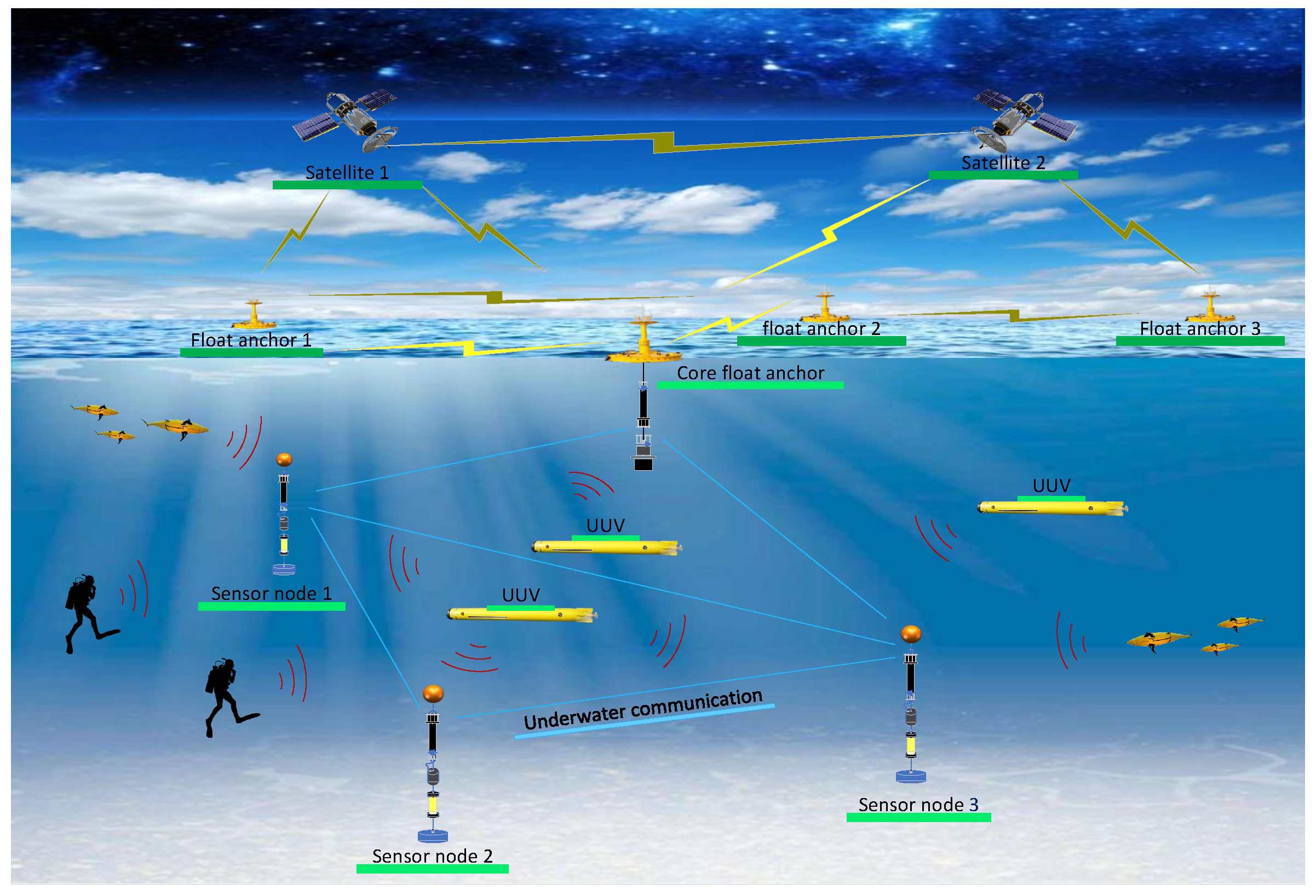
2. System Model
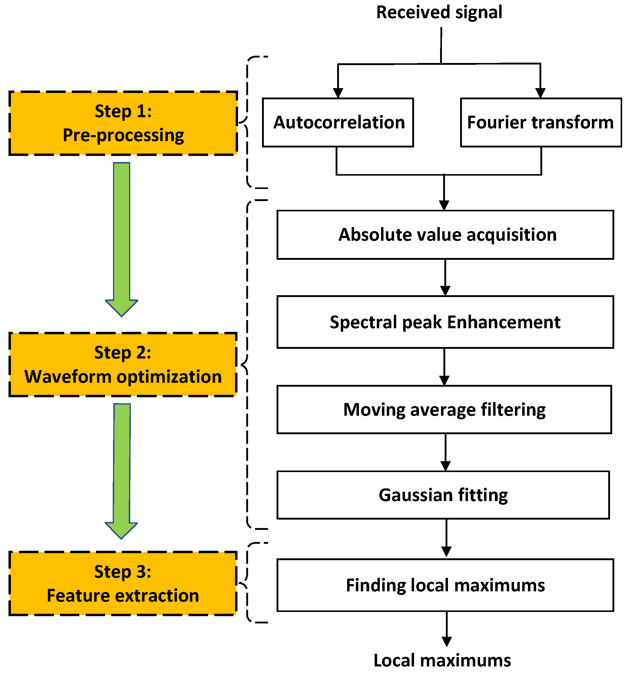
3. Proposed Spectral Peak Feature Extraction Method
3.1. Pre-Processing
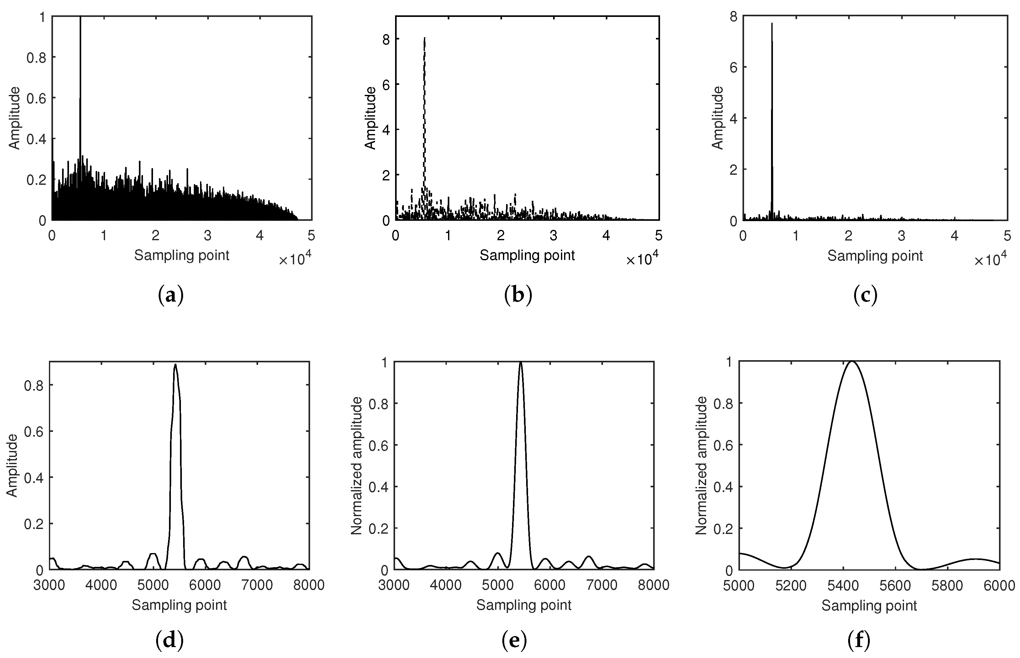
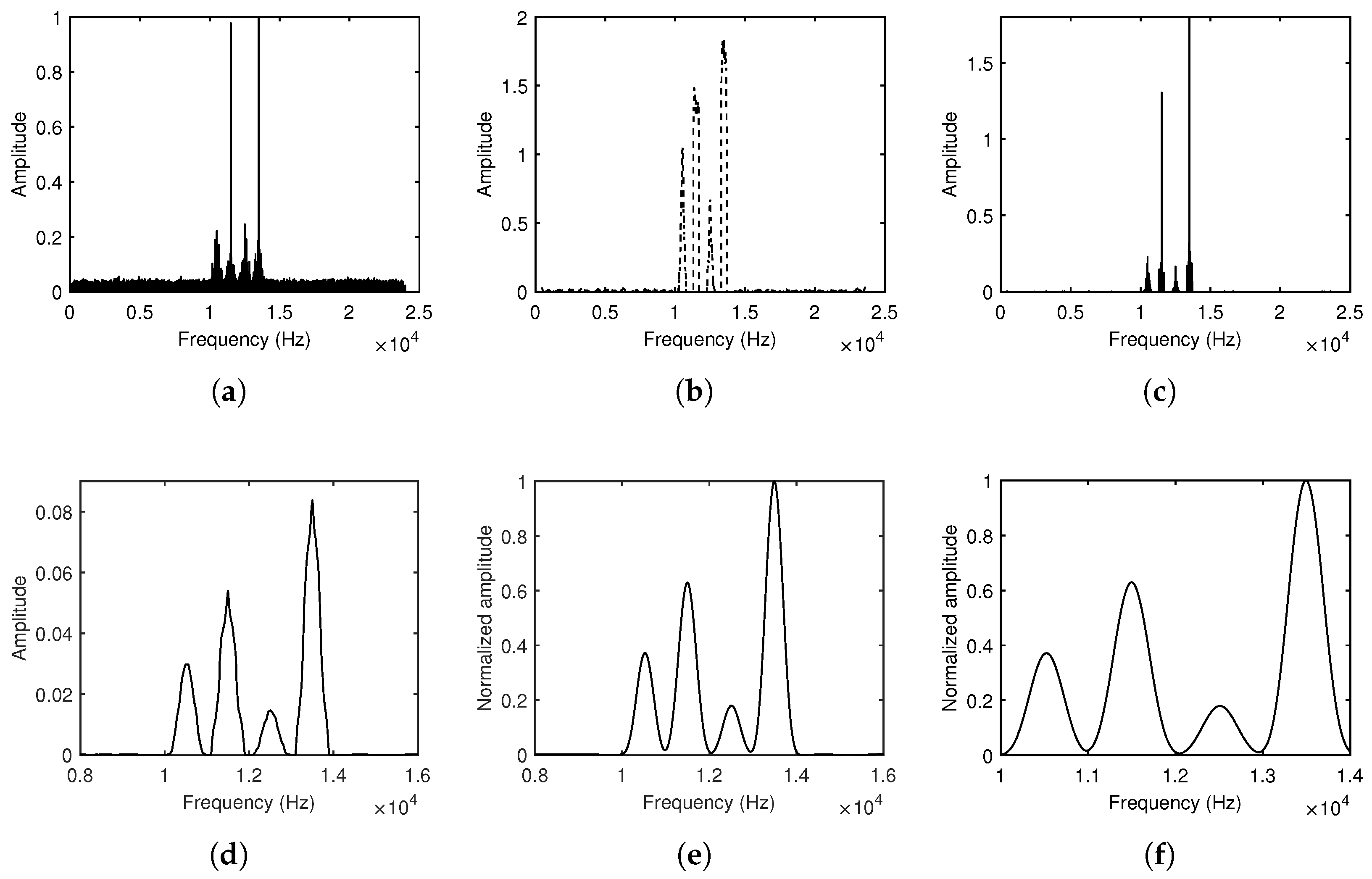
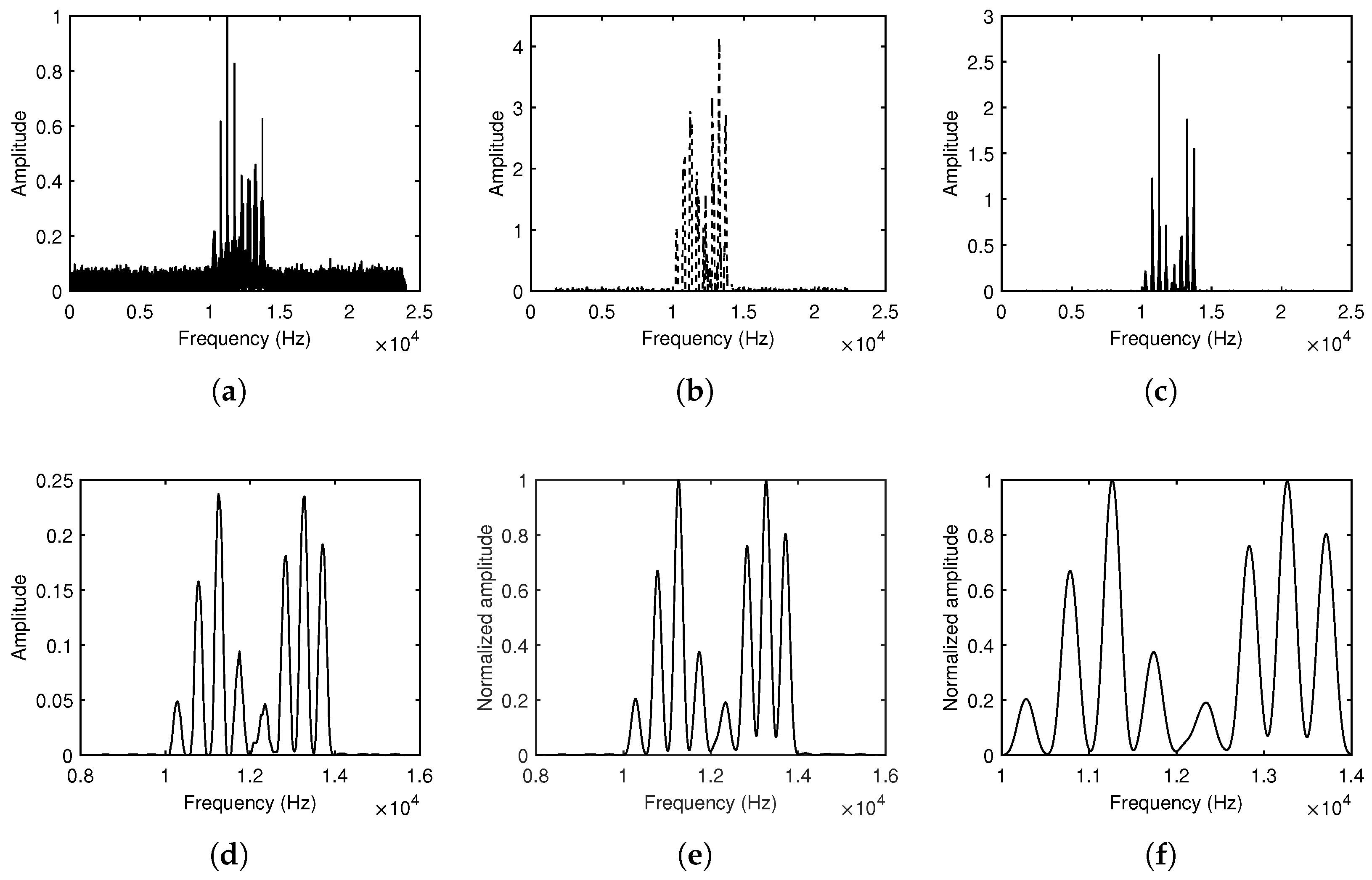
3.2. Waveform Optimization
3.2.1. Absolute Value Acquisition
3.2.2. Spectral Peak Enhancement
3.2.3. Moving Average Filter
3.2.4. Gaussian Fitting
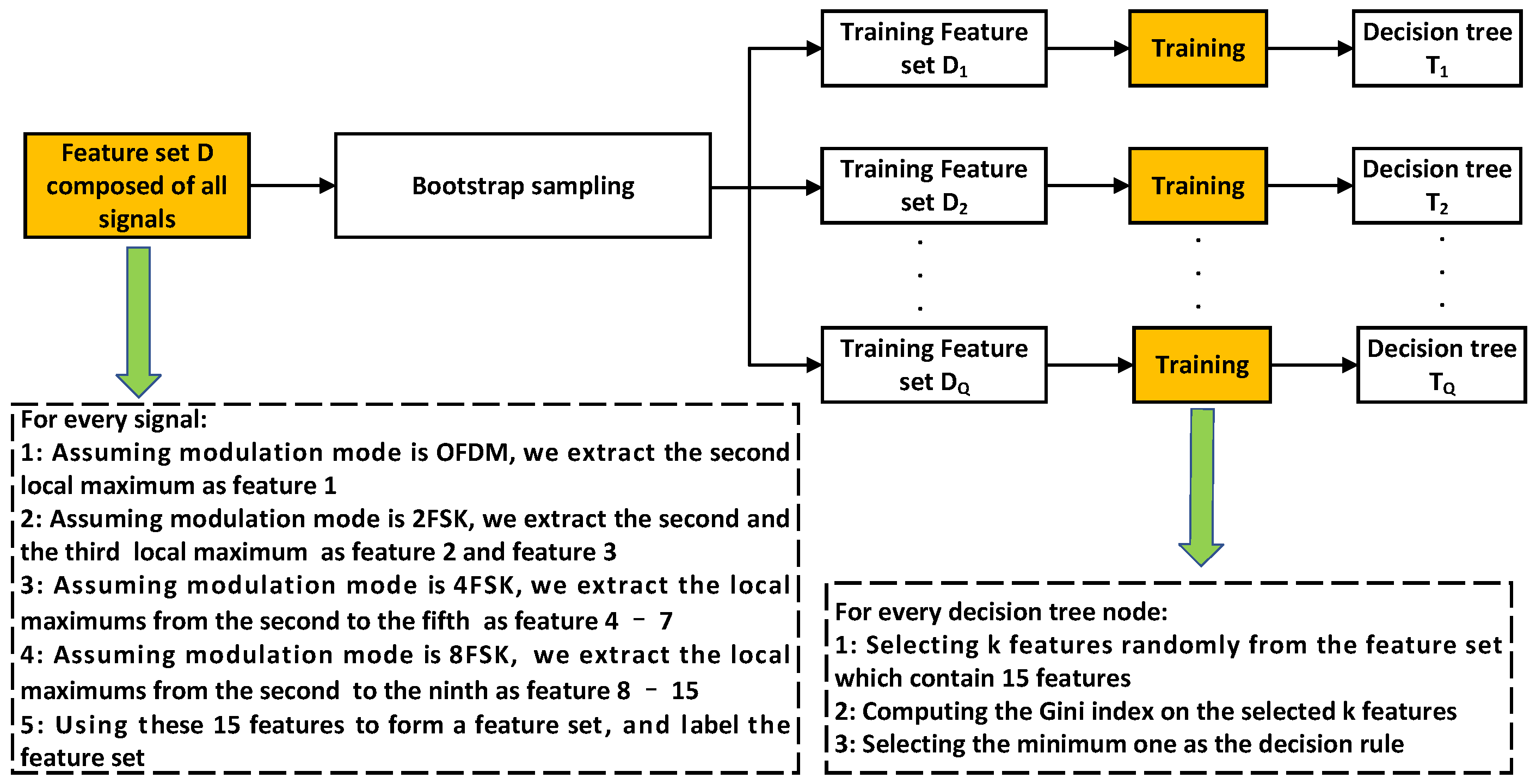
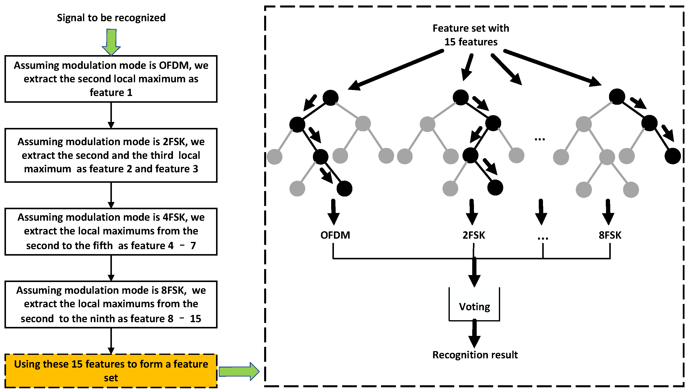
3.3. Feature Extraction
4. RF Classifier
4.1. Classifier Principle
4.2. Complexity Analysis
5. Results
5.1. Simulation Data Analysis
5.1.1. Parameter Setting
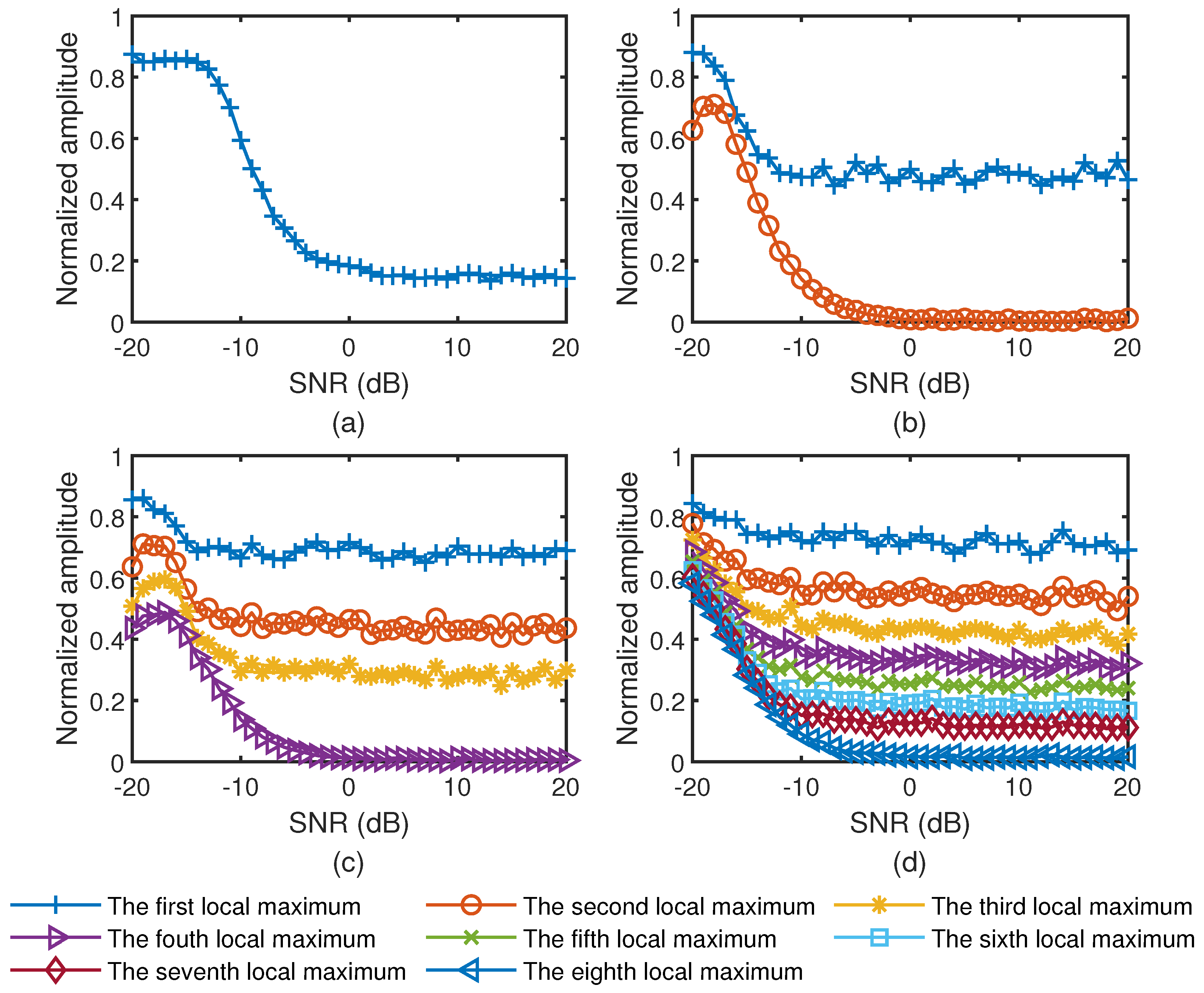
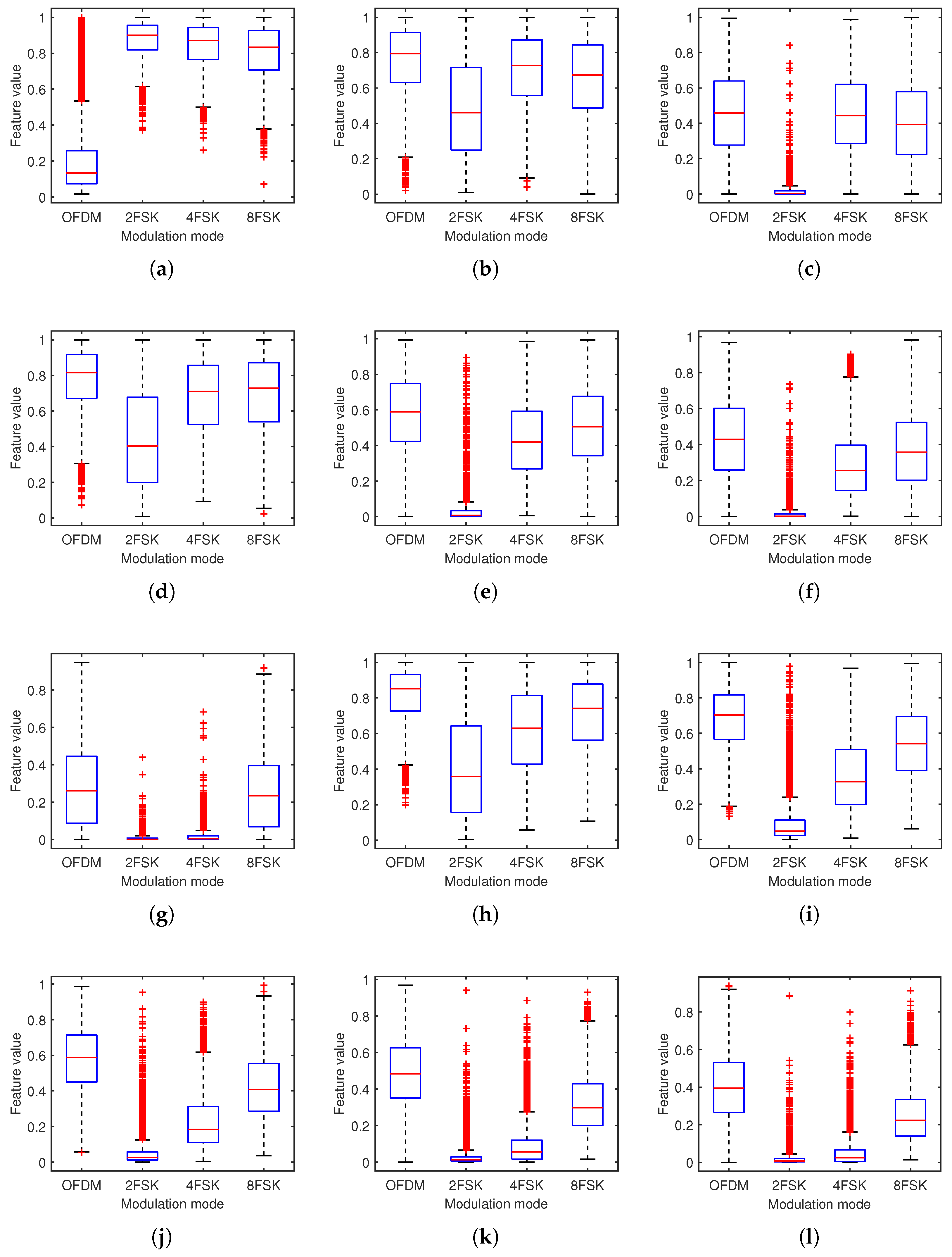
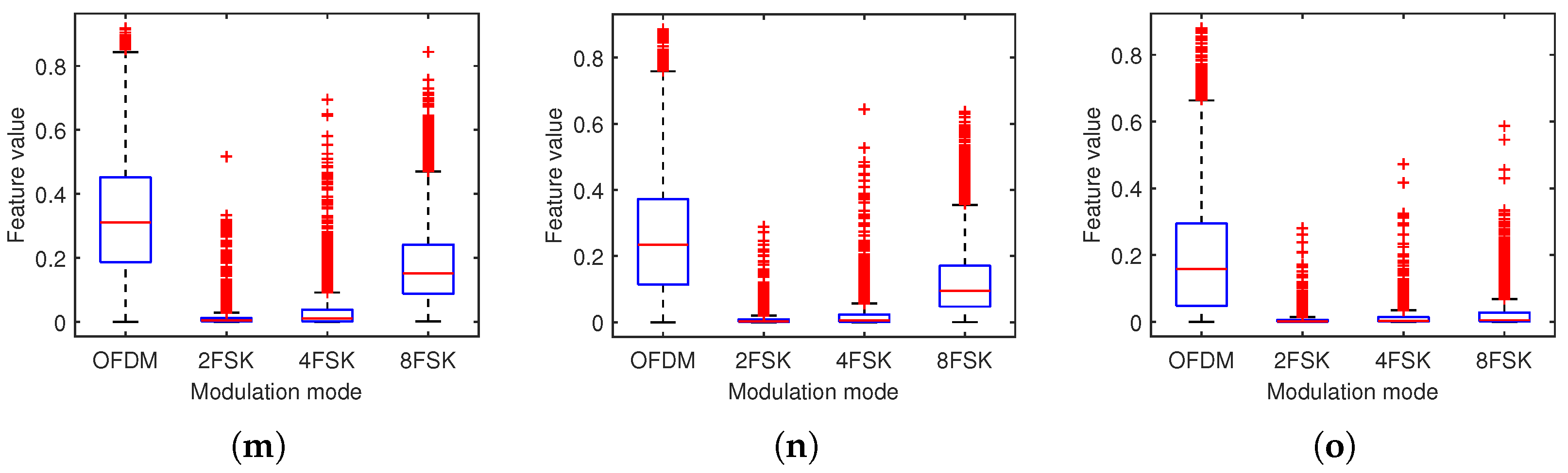
5.1.2. Robustness Analysis of Spectral Peak Features
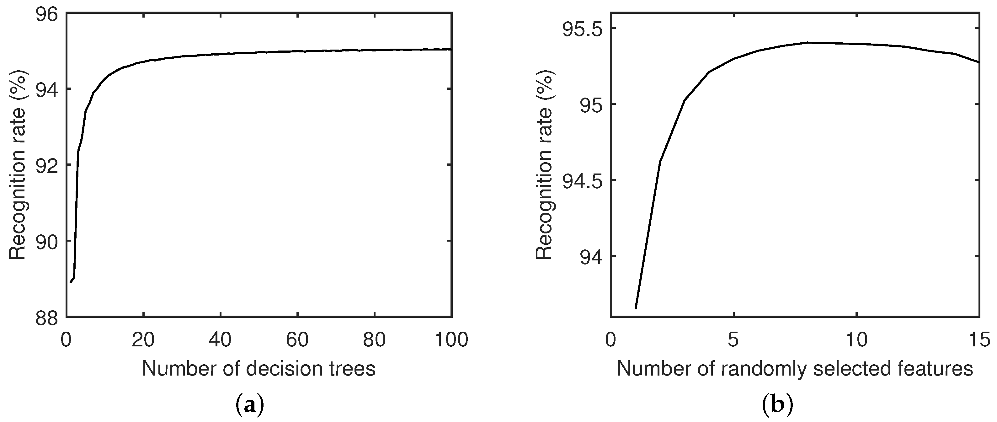
5.1.3. Parameter Determination of the Classifier
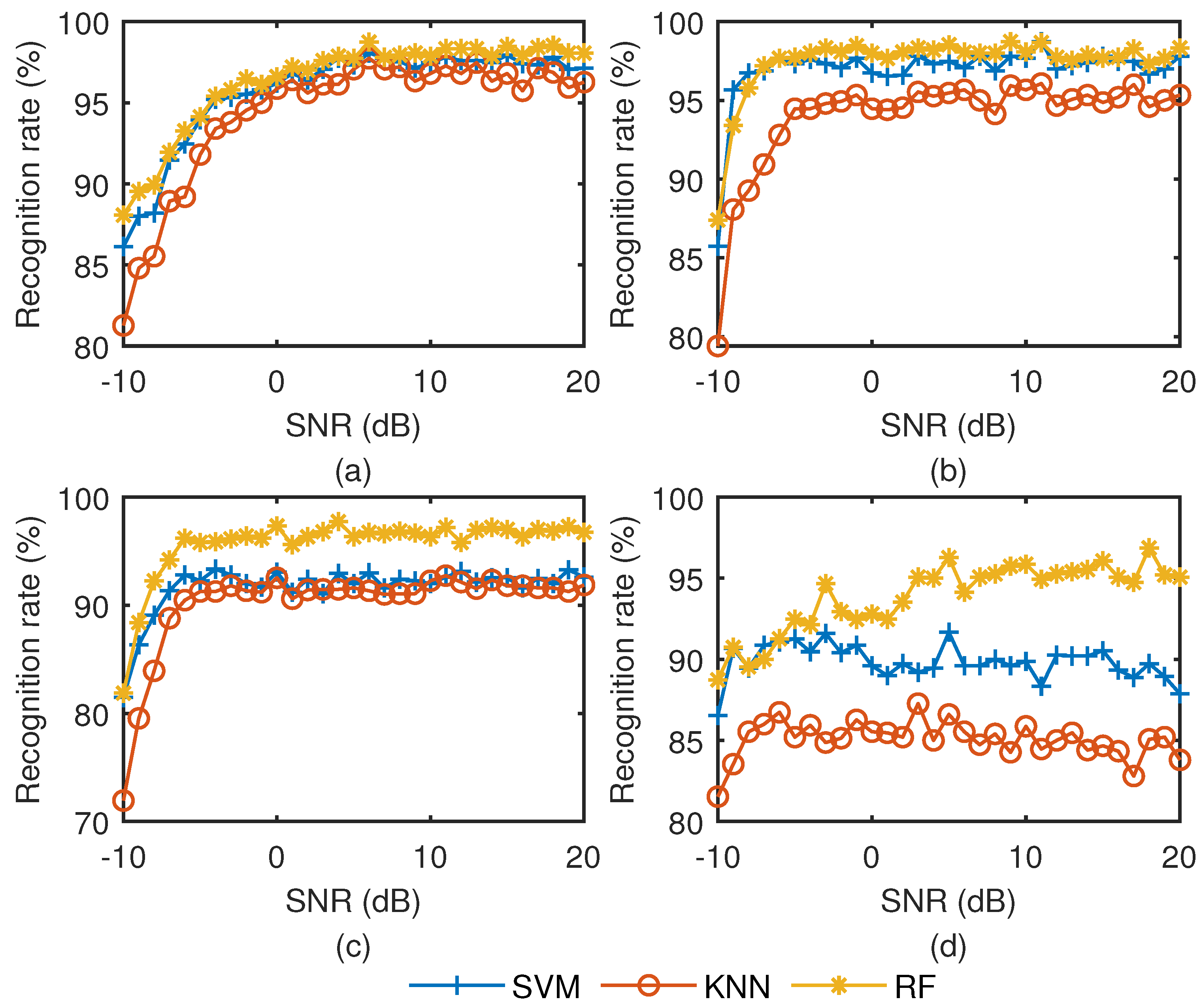
5.1.4. Performance Analysis of The Proposed Method
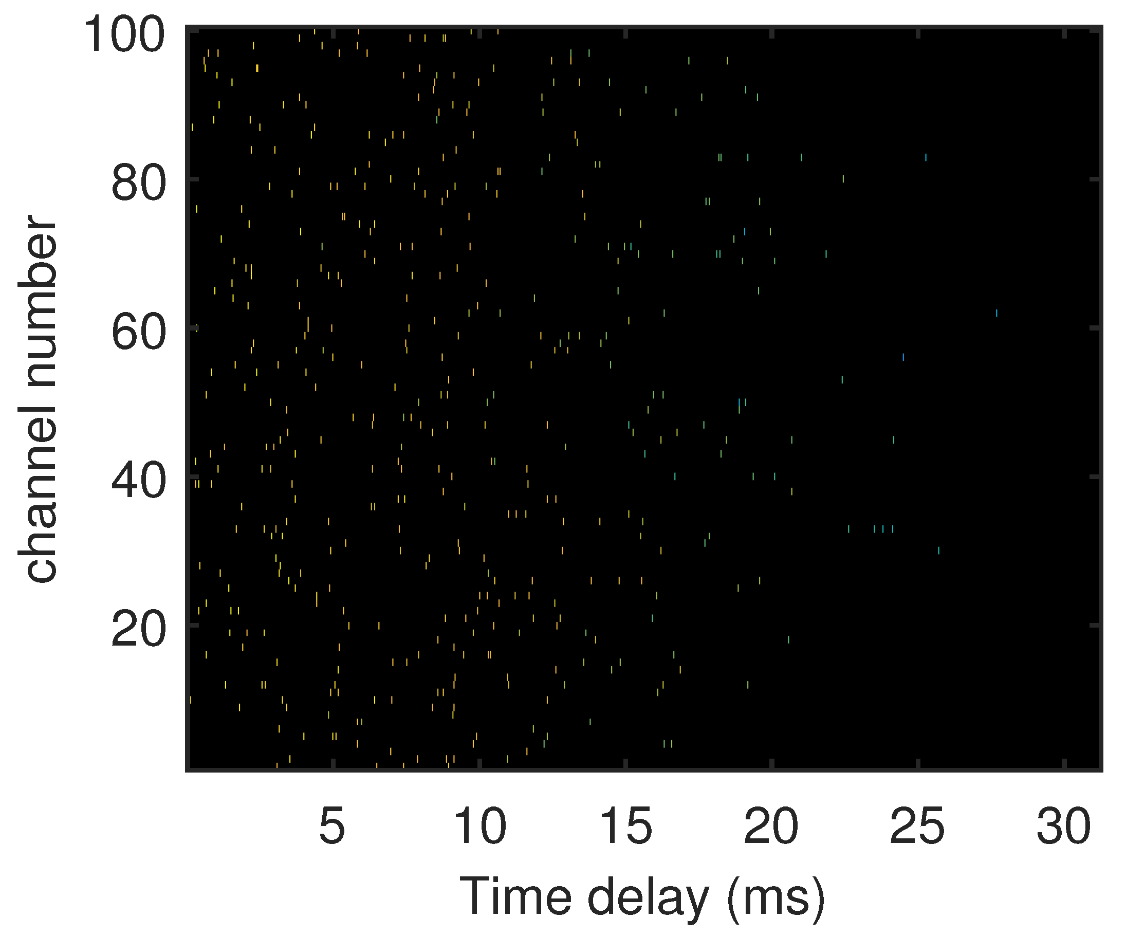
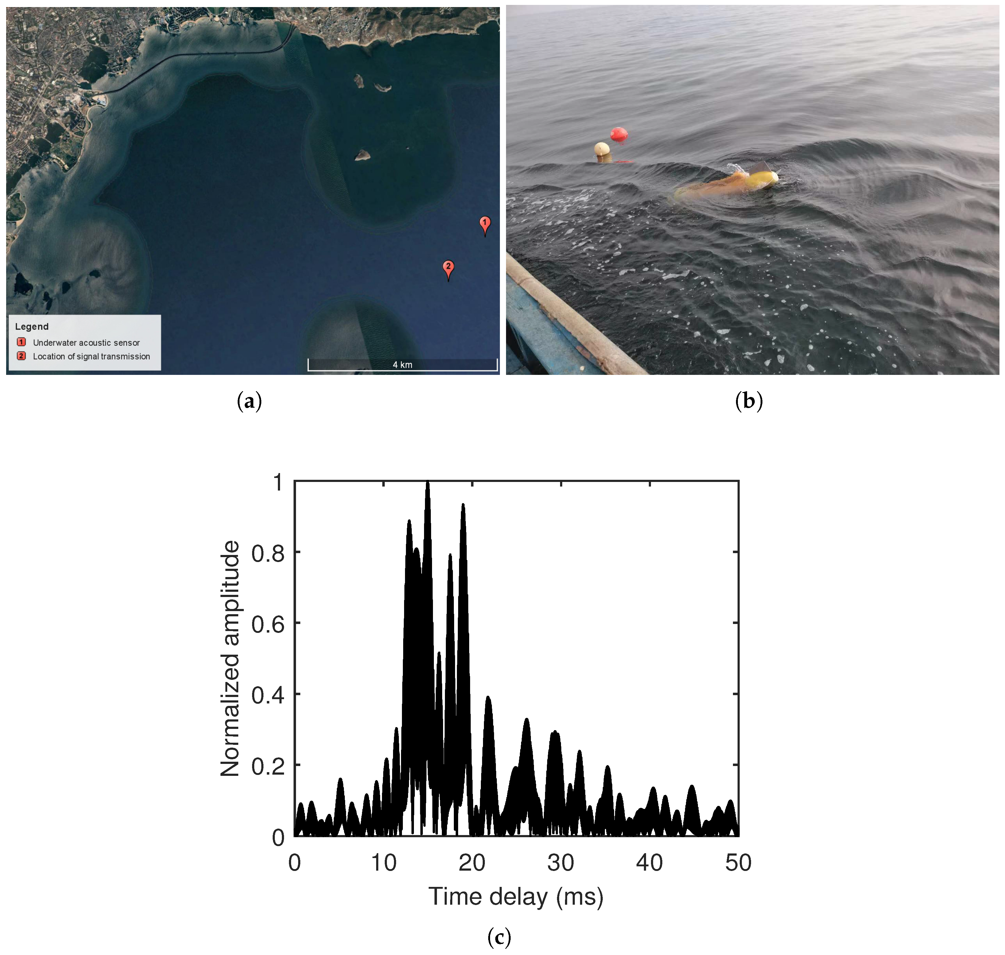
5.2. Experimental Data Analysis
6. Discussion
6.1. Significance of the Proposed Method
6.2. Limitations of the Proposed Method
7. Conclusions
Author Contributions
Funding
Institutional Review Board Statement
Informed Consent Statement
Data Availability Statement
Acknowledgments
Conflicts of Interest
References
- Petrioli, C.; Petroccia, R.; Potter, J.R.; Spaccini, D. The SUNSET framework for simulation, emulation and at-sea testing of underwater wireless sensor networks. Ad Hoc Netw. 2015, 34, 224–238. [Google Scholar] [CrossRef]
- Toso, G.; Masiero, R.; Casari, P. Field Experiments for Dynamic Source Routing: S2C EvoLogics modems run the SUN protocol using the DESERT Underwater libraries. In Proceedings of the MTS/IEEE Oceans Conference, Hampton Roads, VA, USA, 14–19 October 2012; pp. 1–10. [Google Scholar]
- Fang, T.; Liu, S.Z.; Ma, L.; Zhang, L.Y. Subcarrier modulation identification of underwater acoustic OFDM based on block expectation maximization and likelihood. Appl. Acoust. 2021, 173, 107654. [Google Scholar] [CrossRef]
- Fang, T.; Liu, S.Z.; Wu, X.B.; Yan, H.L. Non-cooperative MPSK Modulation Identification in SIMO Underwater Acoustic Multipath Channel. In Proceedings of the 2021 OES China Ocean Acoustics (COA), Harbin, China, 14–17 July 2021; pp. 1–6. [Google Scholar]
- Ren, H.; Yu, J.L.; Wang, Z.X.; Chen, J. Modulation format recognition in visible light communications based on higher order statistics. In Proceedings of the 2017 Conference on Lasers and Electro-Optics Pacific Rim, Sands Expo and Convention Centre, Singapore, 31 July–4 August 2017; pp. 1–2. [Google Scholar]
- Wang, L.X.; Guo, S.T.; Jia, C.J. Modulation format recognition in visible light communications based on higher order statistics. In Proceedings of the 2016 7th IEEE International Conference on Software Engineering and Service Science, Beijing, China, 26–28 August 2016; pp. 627–630. [Google Scholar]
- Li, S.J.; Wang, Y.W. Method of modulation recognition of typical communication satellite signals based on cyclostationary. In Proceedings of the 2013 ICME International Conference on Complex Medical Engineering, Beijing, China, 25–28 May 2013; pp. 268–273. [Google Scholar]
- Wei, Y.J.; Fang, S.L.; Wang, L.Y. Automatic Modulation Classification of Digital Communication Signals Using SVM Based on Hybrid Features, Cyclostationary, and Information Entropy. Entropy 2019, 21, 745. [Google Scholar] [CrossRef] [PubMed] [Green Version]
- Chen, E.; Yan, J.Q.; Sun, H.X. Research on MPSK Modulation Classification of Underwater Acoustic Communication Signals. In Proceedings of the 2016 IEEE/OES China Ocean Acoustics (COA), Harbin, China, 9–11 January 2016; pp. 1–5. [Google Scholar]
- Jiang, W.H.; Chen, D.S.; Wu, Y.Q. Modulation recognition of underwater acoustic OFDM signals based on the correlation property of the cyclic prefix. Appl. Acoust. 2016, 35, 42–49. [Google Scholar]
- Jiang, N.; Wang, B. Underwater Communication Signals’ Modulation Recognition Based on Sparse Autoencoding Network. J. Signal Process. 2019, 35, 103–114. [Google Scholar]
- Jiang, W.H.; Tong, F.; Wang, B. Modulation recognition of non-cooperation underwater acoustic communication signals using principal component analysis. Appl. Acoust. 2016, 37, 1670–1676. [Google Scholar] [CrossRef]
- Wang, M.C.; Liu, J.; Zhang, J.W. Modulation format identification based on phase statistics in Stokes space. Opt. Commun. 2020, 480, 1–7. [Google Scholar] [CrossRef]
- Burges, C.J.C. A Tutorial on Support Vector Machines for Pattern Recognition. Data Min. Knowl. Discov. 1998, 2, 121–167. [Google Scholar] [CrossRef]
- Zhu, Z.C.; Aslam, M.W.; Nandi, A.K. Augmented Genetic Programming for automatic digital modulation classification. In Proceedings of the 2010 IEEE International Workshop on Machine Learning for Signal Processing, Kittila, Finland, 29 August–1 September 2010; pp. 1–6. [Google Scholar]
- Yao, X.H.; Yang, H.H.; Li, Y.Q. Modulation Recognition of Underwater Acoustic Communication Signals based on Convolutional Neural Networks. Unmanned Syst. Technol. 2018, 1, 68–74. [Google Scholar]
- Rakshit, M.; Das, S. An efficient wavelet-based automated R-peaks detection method using Hilbert transform. Biocybern. Biomed. Eng. 2017, 37, 566–577. [Google Scholar] [CrossRef]
- Yuan, L.; Yang, Y.; Hernandez, A. Novel Adaptive Peak Detection Method for Track Circuits Based on Encoded Transmissions. IEEE Sens. J. 2018, 18, 6224–6234. [Google Scholar] [CrossRef]
- Chen, Y.; Yang, K.; Liu, H.L. Self-Adaptive Multi-Peak Detection Algorithm for FBG Sensing Signal. IEEE Sens. J. 2016, 16, 2658–2665. [Google Scholar] [CrossRef]
- Zhou, Z.H. Machine Learning; Tsinghua University Press: Beijing, China, 2016; pp. 73–95, 178–180. [Google Scholar]
- Berger, C.R.; Zhou, S.L.; Preisig, J.C. Sparse Channel Estimation for Multicarrier Underwater Acoustic Communication: From Subspace Methods to Compressed Sensing. IEEE Trans. Signal Process. 2010, 58, 1708–1721. [Google Scholar] [CrossRef] [Green Version]
- Fang, L.; Pascal, D.; Olivier, D. Acoustic Resonance Detection Using Statistical Methods of Voltage Envelope Characterization in Metal Halide Lamps. IEEE Trans. Ind. Appl. 2017, 53, 5988–5996. [Google Scholar]
- Friedman, J.H.; Baskett, F.; Shustek, L.J. An Algorithm for Finding Nearest Neighbors. IEEE Trans. Comput. 1975, C-24, 1000–1006. [Google Scholar] [CrossRef]


| Modulation Mode | Center Frequency | Bandwidth | CP Length | SNR Range | Number of Signals Under Each SNR |
|---|---|---|---|---|---|
| 20 ms | 50 | ||||
| OFDM | 12 kHz | 4 kHz | 30 ms | −20 dB–20 dB, 1 dB increment | 50 |
| 40 ms | 50 | ||||
| 3 kHz | 50 | ||||
| 2FSK | 12 kHz | 4 kHz | - | −20 dB–20 dB, 1 dB increment | 50 |
| 5 kHz | 50 | ||||
| 3 kHz | 50 | ||||
| 4FSK | 12 kHz | 4 kHz | - | −20 dB–20 dB, 1 dB increment | 50 |
| 5 kHz | 50 | ||||
| 3 kHz | 50 | ||||
| 8FSK | 12 kHz | 4 kHz | - | −20 dB–20 dB, 1 dB increment | 50 |
| 5 kHz | 50 |
| Modulation Mode | Center Frequency | Bandwidth | CP Length | SNR Range | Number of Signals Under Each SNR |
|---|---|---|---|---|---|
| 20 ms | 500 | ||||
| OFDM | 12 kHz | 4 kHz | 30 ms | −20 dB–20 dB, 1 dB increment | 500 |
| 40 ms | 500 | ||||
| 3 kHz | 500 | ||||
| 2FSK | 12 kHz | 4 kHz | - | −20 dB–20 dB, 1 dB increment | 500 |
| 5 kHz | 500 | ||||
| 3 kHz | 500 | ||||
| 4FSK | 12 kHz | 4 kHz | - | −20 dB–20 dB, 1 dB increment | 500 |
| 5 kHz | 500 | ||||
| 3 kHz | 500 | ||||
| 8FSK | 12 kHz | 4 kHz | - | −20 dB–20 dB, 1 dB increment | 500 |
| 5 kHz | 500 |
| Modulation Mode | Center Frequency | Bandwidth | CP Length | SNR Range | Number of Signals Under Each SNR |
|---|---|---|---|---|---|
| OFDM | 12 kHz | 4 kHz | 32 ms | 12 dB | 240 |
| 2FSK | 12 kHz | 4 kHz | - | 12 dB | 240 |
| 4FSK | 12 kHz | 4 kHz | - | 12 dB | 240 |
| 8FSK | 12 kHz | 4 kHz | - | 12 dB | 240 |
| Actual | OFDM | 2FSK | 4FSK | 8FSK | |
|---|---|---|---|---|---|
| Predicted | |||||
| SVM: 217(90.42%) | SVM: 1 | SVM: 6 | SVM: 16 | ||
| OFDM | KNN: 208(86.67%) | KNN: 1 | KNN: 7 | KNN: 24 | |
| RF: 219(91.25%) | RF: 3 | RF: 4 | RF: 14 | ||
| SVM: 0 | SVM: 240(100%) | SVM: 0 | SVM: 0 | ||
| 2FSK | KNN: 0 | KNN: 231(96.25%) | KNN: 7 | KNN: 2 | |
| RF: 0 | RF: 240(100%) | RF: 0 | RF: 0 | ||
| SVM: 0 | SVM: 11 | SVM: 224(93.33%) | SVM: 5 | ||
| 4FSK | KNN: 0 | KNN: 13 | KNN: 222(92.50%) | KNN: 5 | |
| RF: 0 | RF: 3 | RF: 233(97.08%) | RF: 4 | ||
| SVM: 0 | SVM: 4 | SVM: 34 | SVM: 202(84.17%) | ||
| 8FSK | KNN: 5 | KNN: 11 | KNN: 58 | KNN: 166(69.17%) | |
| RF: 2 | RF: 0 | RF: 7 | RF: 231(96.25%) | ||
Publisher’s Note: MDPI stays neutral with regard to jurisdictional claims in published maps and institutional affiliations. |
© 2022 by the authors. Licensee MDPI, Basel, Switzerland. This article is an open access article distributed under the terms and conditions of the Creative Commons Attribution (CC BY) license (https://creativecommons.org/licenses/by/4.0/).
Share and Cite
Fang, T.; Wang, Q.; Zhang, L.; Liu, S. Modulation Mode Recognition Method of Non-Cooperative Underwater Acoustic Communication Signal Based on Spectral Peak Feature Extraction and Random Forest. Remote Sens. 2022, 14, 1603. https://doi.org/10.3390/rs14071603
Fang T, Wang Q, Zhang L, Liu S. Modulation Mode Recognition Method of Non-Cooperative Underwater Acoustic Communication Signal Based on Spectral Peak Feature Extraction and Random Forest. Remote Sensing. 2022; 14(7):1603. https://doi.org/10.3390/rs14071603
Chicago/Turabian StyleFang, Tao, Qian Wang, Lanyue Zhang, and Songzuo Liu. 2022. "Modulation Mode Recognition Method of Non-Cooperative Underwater Acoustic Communication Signal Based on Spectral Peak Feature Extraction and Random Forest" Remote Sensing 14, no. 7: 1603. https://doi.org/10.3390/rs14071603