Article

MLCRNet: Multi-Level Context Refinement for Semantic Segmentation in Aerial Images

School of Computer Science and Technology, East China Normal University, Shanghai 200062, China
*
Author to whom correspondence should be addressed.
Remote Sens. 2022, 14(6), 1498; https://doi.org/10.3390/rs14061498
Submission received: 14 February 2022 / Revised: 16 March 2022 / Accepted: 17 March 2022 / Published: 20 March 2022
(This article belongs to the Topic Computational Intelligence in Remote Sensing)

Abstract

:
In this paper, we focus on the problem of contextual aggregation in the semantic segmentation of aerial images. Current contextual aggregation methods only aggregate contextual information within specific regions to improve feature representation, which may yield poorly robust contextual information. To address this problem, we propose a novel multi-level context refinement network (MLCRNet) that aggregates three levels of contextual information effectively and efficiently in an adaptive manner. First, we designed a local-level context aggregation module to capture local information around each pixel. Second, we integrate multiple levels of context, namely, local-level, image-level, and semantic-level, to aggregate contextual information from a comprehensive perspective dynamically. Third, we propose an efficient multi-level context transform (EMCT) module to address feature redundancy and to improve the efficiency of our multi-level contexts. Finally, based on the EMCT module and feature pyramid network (FPN) framework, we propose a multi-level context feature refinement (MLCR) module to enhance feature representation by leveraging multi-level contextual information. Extensive empirical evidence demonstrates that our MLCRNet achieves state-of-the-art performance on the ISPRS Potsdam and Vaihingen datasets.

1. Introduction

Image segmentation or semantic annotation is an exceptionally significant topic in remote sensing image interpretation and plays a key role in various real-world applications, such as geohazard monitoring [1,2], urban planning [3,4], site-specific crop management [5,6], autonomous driving systems [7,8], and land change detection [9]. This task aims to segment and interpret a given image into different image regions associated with semantic categories.
Recently, deep learning methods represented by deep convolutional neural networks [10] have demonstrated powerful feature extraction capabilities compared with traditional feature extraction methods, thereby sparking the interest of researchers and prompting a series of works [11,12,13,14,15,16]. Among these works, FCN [11] is a pioneer in deep convolutional neural networks and has made great progress in the field of image segmentation. Its encoder–decoder architecture first employs several down-sampling layers in the encoder to reduce the spatial resolution of the feature map to extract features. Then, it uses several up-sampling layers in the decoder to restore the spatial resolution, and it exhibits many improvements in semantic segmentation. However, limited by the structure of the encoder–decoder, FCN suffers from inadequate contextual and detail information. On one hand, some of the detail information is usually dropped by the down-sampling operation. On the other hand, due to the inherent nature of convolution, FCN does not provide adequate contextual information. This task leaves plenty of room for improvement. The key to improving the performance of semantic segmentation is to obtain strong semantic representation with detail information (e.g., detailed target boundaries, location, etc.) [17].
To restore detail information, several studies fuse features that come from encoder (low-level features) and decoder (high-level features) by long-range skip connections. FPN-based approaches [18,19,20] employ a long-range lateral path to refine feature representations across layers iteratively. SFNet [17] extracts location information from low-level features at a limited scope (e.g., 3 × 3 kernel size) and then applies it to calibrate the target boundaries of high-level features. Although impressive, these methods solely focus on harvesting contextual information from a local perspective (the local level) and do not aggregate contextual information from a more comprehensive perspective.
Furthermore, to improve the intra-class consistency of feature representation, some studies enhance feature representation by aggregating contextual information. Wang et al. [21] proposed the self-attention mechanism, a long-range contextual relationship modeling approach that is used by the segmentation model [22,23,24,25] to aggregate contextual information across an image adaptively. EDFT [26] designed the Depth-aware Self-attention (DSA) Module, which uses the self-attention mechanism to aggregate image-level contextual information to merge RGB features and depth features. Nevertheless, these approaches only focus on harvesting contextual information from the perspective of the whole image (the image level) without explicit guidance of prior context information [27], and they suffer from high computational complexity O ( ( H W ) 2 ) , where H W is the input image size [28]. In addition, OCRNet [29], ACFNet [30], and SCARF [31] model the contextual relationships within a specific category region based on coarse segmentation (the semantic level). However, in some regions, the contextual information tends to be unbalanced (e.g., pixels in the border or small-scale object regions are susceptible to interference from another category), leading to the misclassification of these pixels. Moreover, ISNet [32] models contextual information from the perspective of the image level and semantic level. HMANet [33] designed a Class Augmented Attention (CAA) module to capture semantic-level context information and a Region Shuffle Attention (RSA) module to exploit region-wise image level context information. Although these methods improve the intra-class consistency of the feature representation, they still lack local detail information, resulting in lower classification accuracy in the object boundary region.
Several works have attempted to combine local-level and image-level contextual information to enhance the detail information and intra-class consistency of feature maps. MANet [34] introduces the multi-scale context extraction module (MCM) to extract both local-level and image-level contextual information in low-resolution feature maps. Zhang et al. [35] aggregate local-level contextual information in a high-resolution branch and harvest image-level contextual information in a low-resolution branch based on HRNet. HRCNet [36] proposes a light-weight dual attention (LDA) module to obtain image-level contextual information, and then the feature enhancement feature pyramid (FEFP) module is designed to exploit the local-level and image-level contextual information in parallel structure. Although these methods harvest local-level and image-level contextual information within the single module or between different modules, they are still missing the contextual dependencies of distinct classes. This paper seeks to provide a solution to these issues by integrating different levels of contextual information efficiently to enhance feature representation.
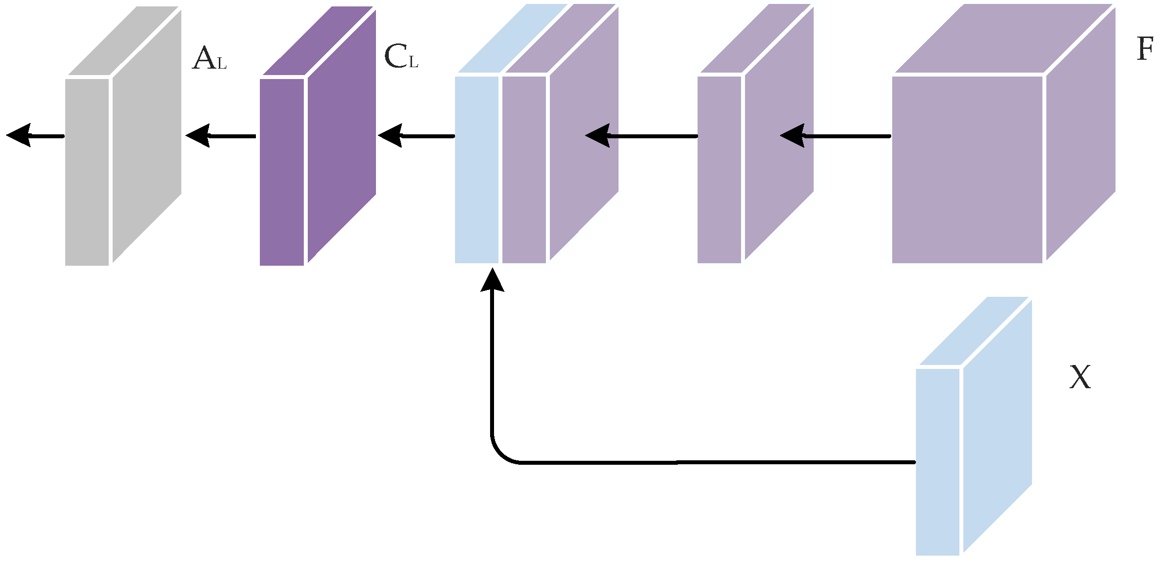
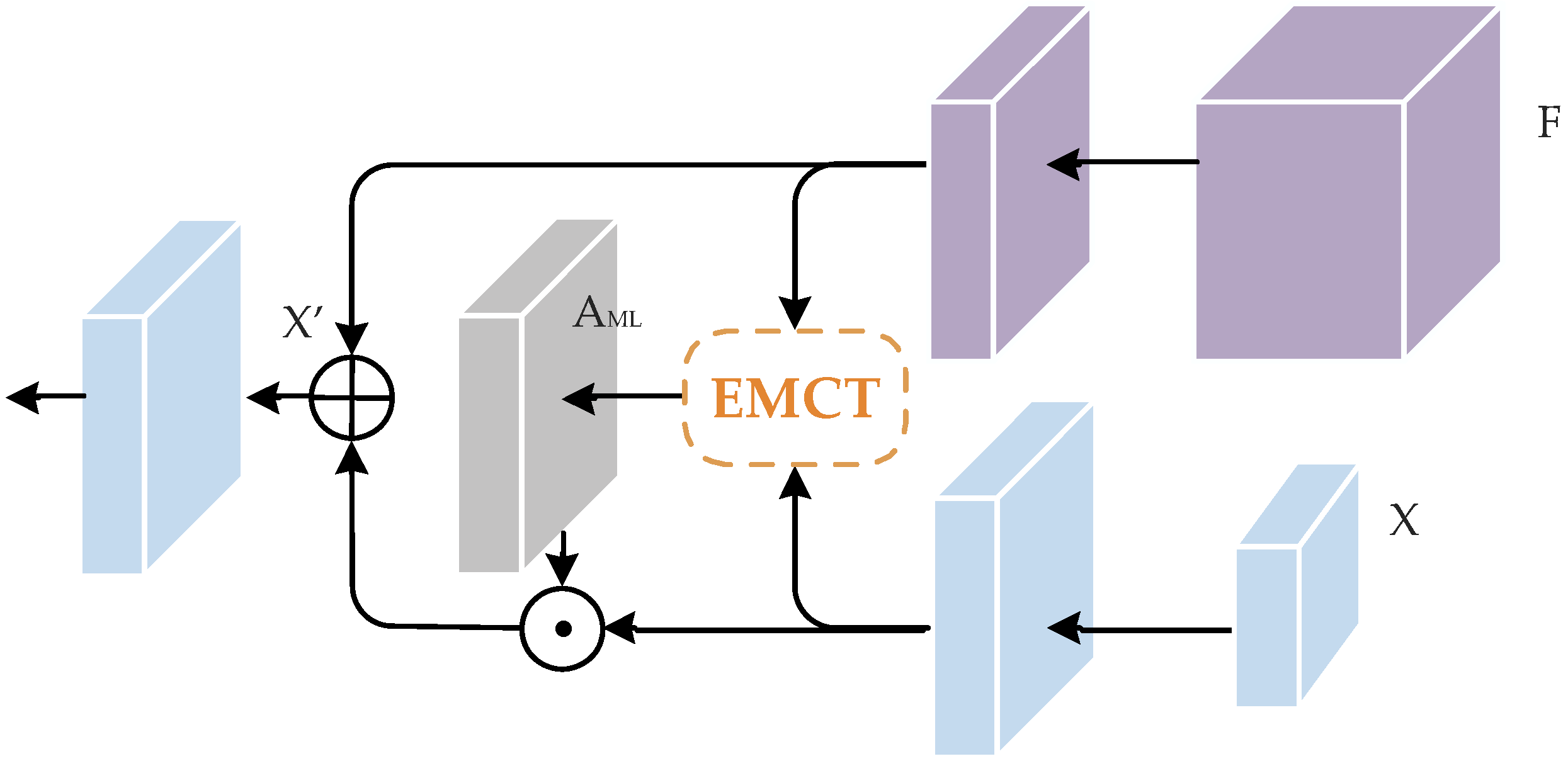
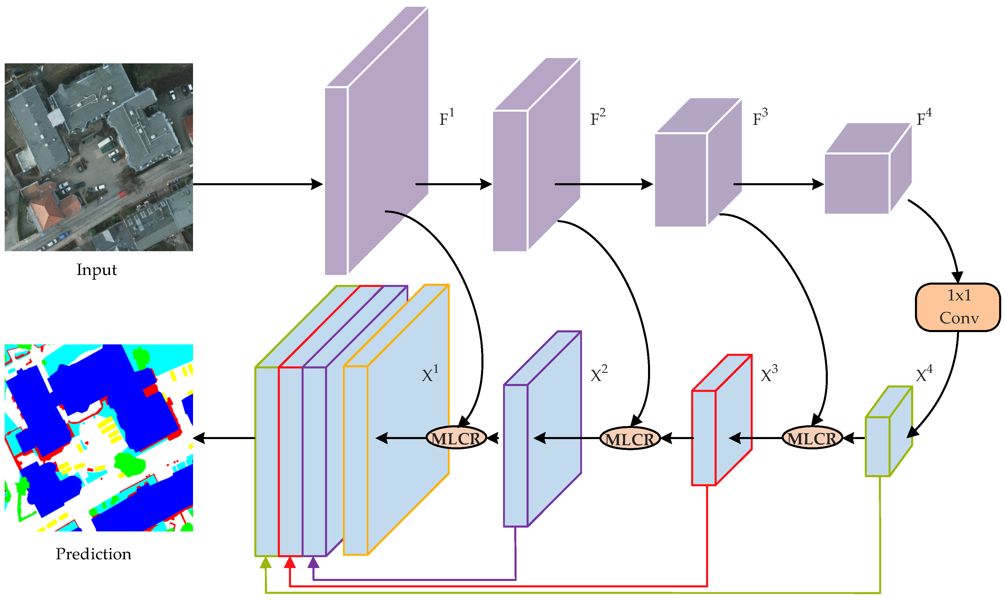
To this end, we propose a novel network called the multi-level context refinement network (MLCRNet) to harvest contextual information from a more comprehensive perspective efficiently. The basic idea is to embed local-level and image-level contextual information into semantic-level contextual relations to obtain more comprehensive and accurate contextual information to augment feature representation. Specifically, inspired by the flow alignment module in SFNet [17], we first design a local-level context aggregation module, which discards the warp operation that demands extensive computation and enhances the feature representation with a local contextual relationship matrix directly. Then, we propose the multi-level context transform (MCT) module to integrate three levels of context, namely, local-level, image-level, and semantic-level, to capture contextual information from multiple aspects adaptively, which can improve model performance but dramatically increased GPU memory usage and inference time. Thus, an efficient MCT (EMCT) module is presented to address feature redundancy and to improve the efficiency of our MCT module. Subsequently, based on the EMCT block and FPN framework, we propose a multi-level context prior feature refinement module called the multi-level context refinement (MLCR) module to enhance feature representation by aggregating multi-level contextual information. Finally, our model refines the feature map iteratively across FPN [18] decoder layers with MLCR.
In summary, our contribution falls into three aspects:
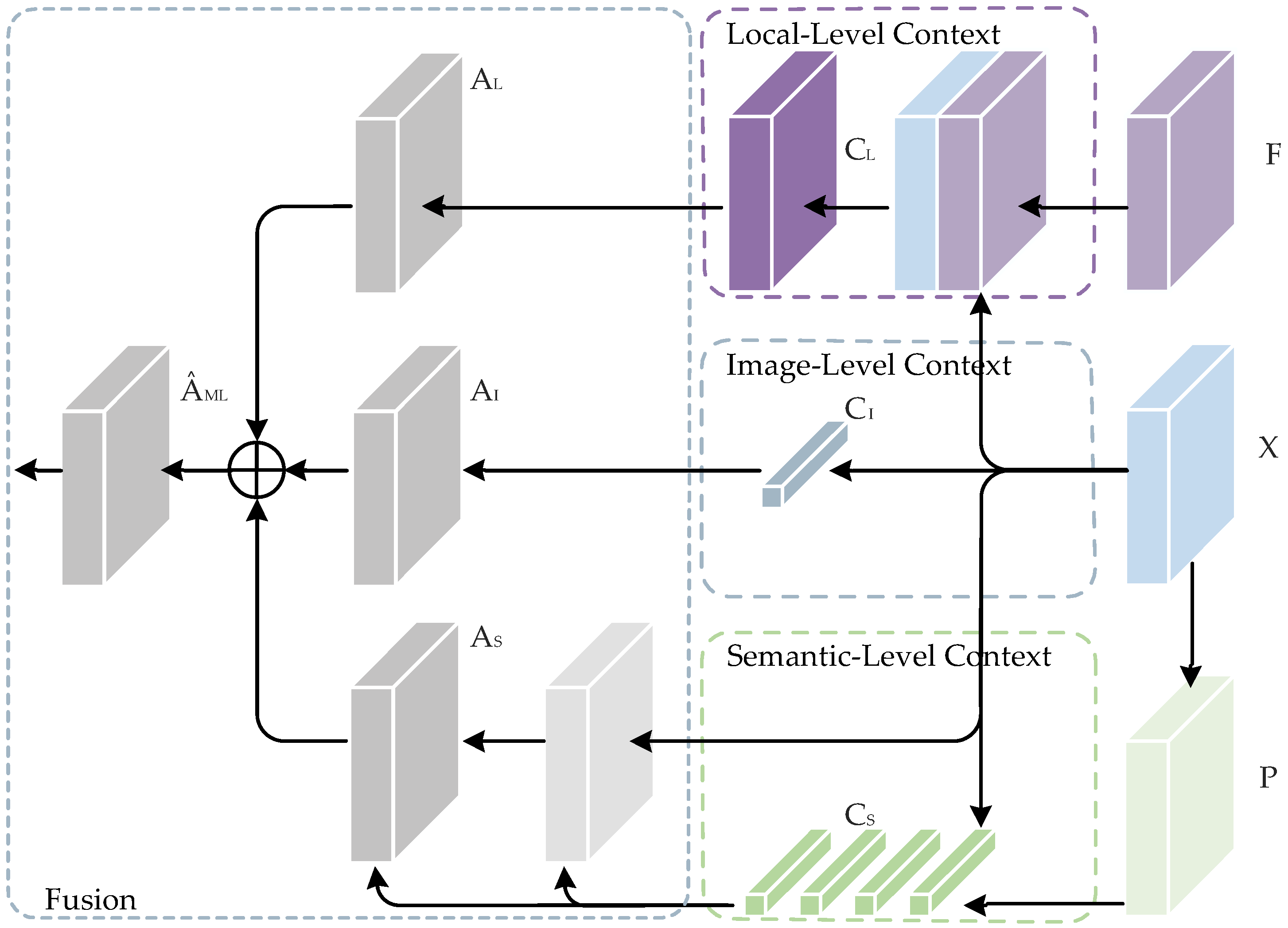
  • We propose a MCT module, which dynamically harvests contextual information from the semantic, image, and local perspectives.
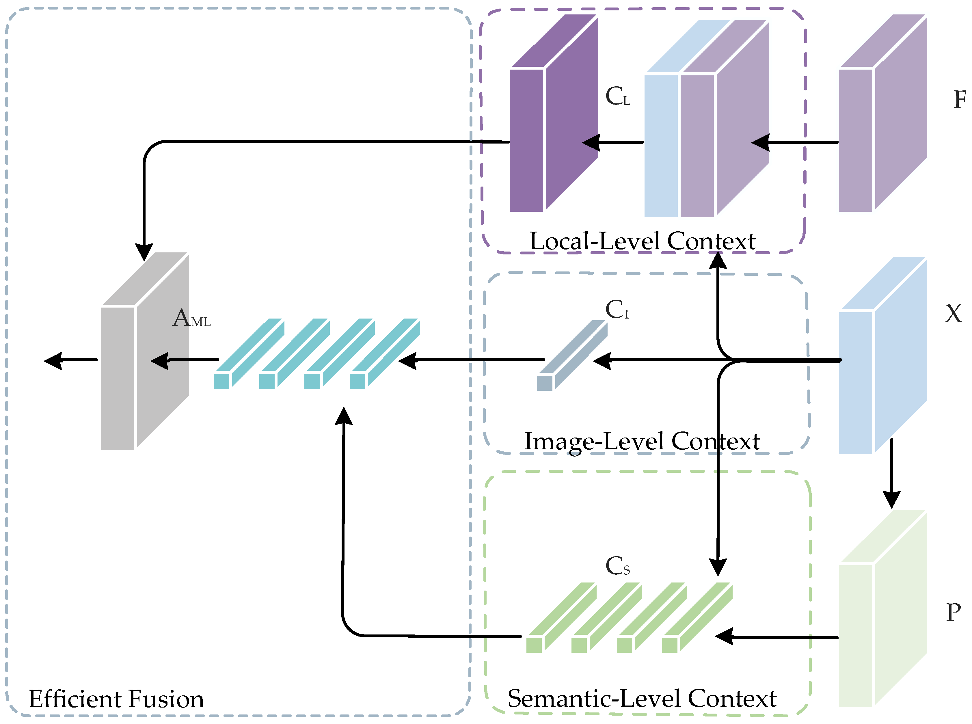
  • The EMCT module is designed to address feature redundancy and improve the efficiency of our MCT module. Furthermore, a MLCR module is proposed on the basis of EMCT and FPN to enhance feature representation by aggregating multi-level contextual information.
  • We propose a novel MLCRNet based on the feature pyramid framework for accurate semantic segmentation.

2. Related Work

2.1. Semantic Segmentation

Over the past decade, deep learning methods represented by convolutional neural networks have made substantial advances in the field of semantic segmentation. FCN is a seminal work that applies convolutional layers on the entire image to replace fully connected layers to generate pixel-by-pixel labels, and many researchers have made great improvements based on it. These improvements can be roughly divided into two categories. One is for encoders to improve the robustness of feature representation. Yu et al. [37] designed an efficient structure called STDC for the semantic segmentation task, which obtains variant scalable receptive fields with a small number of parameters. HRNet [38] obtains a strong semantic representation with detail information by parallelizing multiple branches with different spatial resolutions. The other improvement is for the decoder, which introduces richer contextual information to enhance feature representation. DeepLab [13,14,15] presents the ASPP module that collects multi-scale contexts by employing a series of convolutions with different dilation rates. SENet [39] harvests global contexts by using global average pooling (GAP), and GCNet [40] adopts query-independent attention to model global contexts. This work concentrates on the latter, which aggregates more robust contextual information to enhance feature representation.

2.2. Context Aggregation

Based on the scope of context modelling, we can roughly categorize these contextual aggregation methods into three categories, namely, local level, image level, and semantic level. OCRNet [29], ACFNet [30], and SCARF [31] model contextual relationships within a specific category region based on coarse segmentation results. FLANe [41] and DANet [22] use self-attention [21] to gather image-level contexts along channel and spatial dimensions. Li et al. [42] present a kernel attention with linear complexity to capture image-level context in the spatial dimension. ISANet [43] disentangles dense image-level contexts into the product of two sparse affinity matrices. CCNet [44] iteratively collects contextual information at a criss-cross pathway to approximate image-level contextual information. PSPNet [45] and DeepLab [13,14,15] harvest context at multiple scales, and SFNet [17] harvests local-level contextual information by using the flow alignment module.

2.3. Semantic Segmentation of Aerial Imagery

Unlike natural images, the use of semantic segmentation in aerial images is more challenging. Niu et al. [33] proposed hybrid multiple attention (HMA), which models attention in channel, spatial, and category dimensions to augment feature representation. Yang et al. [46] designed a collaborative network for image super-resolution and the segmentation of remote sensing images, which takes low-resolution images as input to obtain high-resolution semantic segmentation and super-resolution image reconstruction results, thereby effectively alleviating the constraints of inconvenient high-resolution data as well as limited computational resources. Saha et al. [47] proposed a novel unsupervised joint segmentation method, which separately feeds multi-temporal images to a deep network, and the segmentation labels are obtained from the argmax classification of the final layer. Du et al. [48] proposed an object-constrained higher-order CRF model to explore local-level and semantic-level contextual information to optimize segmentation results. EANet [49] combines aerial image segmentation with edge prediction tasks in a multi-task learning approach to improve the classification accuracy of pixels in object contour regions.

3. Methods

3.1. General Contextual Refinement Framework

As shown in Figure 1, the general contextual refinement scheme can be divided into three parts, namely, context modeling, transformation, and weighting:
C = f c ( X )
A = f t ( C )
X = f w ( A , g ( X ) )
where X R D is the input feature map, f c is the contextual information aggregate function, C is the context relation matrix, function f t is adopted to transform context relation into context the attention matrix A R D , f w is the weighting function, and X R D is the output feature map. The function g is used to calculate a better embedding of the input feature map. In this paper, we take g as part of f w and set g as identity embedding: g ( x ) = x .
According to the different context modelling methods, the generic definition can be divided into three specific examples, namely, local-level context, image-level context, and semantic-level context.

3.1.1. Local-Level Context

The main purpose of proposed local-level context is to calibrate misalignment pixels between fine and coarse feature maps from the encoder and decoder. Concretely, standard encoder–decoder semantic segmentation architecture relies heavily on up-sampling methods to up-sample the low spatial resolution strong semantic feature maps into high spatial resolution. However, the widely used up-sampling approaches, such as bilinear up-sampling, can not recover spatial detail information, which is lost during the down-sampling process. Therefore, the misalignment problem must be solved by utilizing the precise position information from the encoder feature map. As depicted in Figure 2, we first harvest local-level context information C L :
C L = ζ ( C a t ( τ ( F ) , β ( X ) ) )
where F R C × H W is a C -dimensional feature map from the encoder; X R C × H × W is the decoder feature map; τ and β are used to compress the channel depth of F and X to be the same, respectively; C a t represents the channel concatenation operation; ζ is implemented by one 3 × 3 convolutional layer; C L R K × H W ; and K is the category number. Then, C L is transformed into the local-level context attention matrix A L :
A L = φ ( C L ) ,
where φ is the local-level context transformation function and implemented by one 1 × 1 convolutional layer, and A L R C × H W .

3.1.2. Image-Level Context

The main purpose of the image-level context is to model the contextual information from the perspective of the whole image [32]. Here, we adopt the GAP operation to gather image-level prior context information C I :
C I = ρ ( G A P ( X ) )
where ρ is implemented by two 1 × 1 convolutional layer, and C I R C × 1 . Then, r e p e a t is adopted to generate the image-level context attention matrix A I :
A I = r e p e a t ( C I )
where A I R C × H W is the image-level context attention matrix.

3.1.3. Semantic-Level Context

The central idea of semantic-level context is to aggregate contextual information based on semantic-level prior information [29,30,31]. We first employ an auxiliary segmentation head ξ and class dimension normalized exponential function S o f t m a x to predict the category posterior probability distribution P :
P = S o f t m a x ( ξ ( X ) )
where X R C × H W ( C , H , and W stand for the number of channels, height, and width of the feature map, respectively), and P R K × H W (K is the number of semantic categories). Then, we aggregate the semantic prior context C S according to the category posterior probability distribution:
C S = X P T
where C S R C × K is the semantic-level contextual information. Finally, we apply self-attention to generate the semantic-level context attention matrix A S :
A S = η ( C S ) S o f t m a x ( ϕ ( C S T ) ψ ( X ) d )
where A S R C × H W is the semantic-level context attention matrix, η ,   ϕ ,   and   ψ are embeddings implemented by two 1 × 1 convolutional layer, and d is the number of the middle channel.

3.2. EMCT

The intuition of the proposed EMCT is to efficiently and dynamically extract contextual information from the category, image, and local perspectives.

3.2.1. Multi-Level Context Transform

The most straightforward way to transform multi-level contextual information is to directly sum up all levels’ context attention matrices. As shown in Figure 3, we propose a multi-level context transformation block, called MCT block, which first computes the local-level, image-level and semantic-level contextual attention matrices separately, and then directly sums them together to obtain the multi-level contextual attention matrix:
A ^ M L = r e s h a p e ( A L + A I + A S )
where A L R C × H W , A I R C × H W , and A S R C × H W are the local-level, image-level and semantic-level contextual attention matrices mentioned in Section 3.1, r e s h a p e is adopted to switch the dimension of the multi-level context attention matrix to R C × H × W , and A ^ M L R C × H × W is the multi-level context attention matrix.

3.2.2. Reduction of Computational Complexity

To alleviate contextual information redundancy and reduce computational complexity, we design an EMCT module by reframing the context transform operation based on the MCT block. As illustrated in Figure 4, we construct the EMCT block as:
A M L = ( C S C I ) C L
where A M L R C × H × W and is the broadcast element-wise multiplication that we use to embed image-level contextual information into semantic level contextual information. Then, we further fuse it with the local contextual information matrix C L by matrix multiplication to generate the multi-level contextual relationship matrix A M L . Our designed EMCT module outperforms the MCT module in terms of time complexity and space complexity. Detailed complexity comparison results are presented in Section 4.2.4.

3.3. Multi-Level Context Refinement Module

Based on the EMCT block, we propose a multi-level context feature refinement module called the MLCR module. According to Figure 5, we construct the MLCR block as:
X = [ E M C T ( U p s a m p l e 2 × ( X ) , F ) U p s a m p l e 2 × ( X ) ] F
where F R C × H × W is the fine feature map from the encoder, X R C × H / 2 × W / 2 is the prior decoder layer output, U p s a m p l e 2 × is the bilinear up-sample operation, stands for the broadcast element-wise addition, and X is the refined feature map.

3.4. MLCRNet

Finally, we construct a coarse-to-fine network based on the MLCR module called MLCRNet (Figure 6). MLCRNet incorporates the backbone network and FPN decoder, and any standard classification network with four stages (e.g., ResNet series [16,50,51]) can serve as the backbone network. The FPN [18] decoder progressively fuses high-level and low-level features by bilinear up-sampling to build up a hierarchical multi-scale pyramid network. As shown in Figure 6, the decoder can be seen as an FPN armed with multiple MLCRs.
Initially, we feed the input image I R 3 × H × W into the backbone network and projected it to a set of feature maps { F s } s [ 1 , 4 ] from each network stage, where F s R C s × H s × W s denotes the i-th stage of the backbone output, H s = H 2 s + 1 , and W s = W 2 s + 1 . Then, considering the complexity of the aerial image segmentation task and the overall network computation cost, we replace the 4th stage of the FPN [18] decoder with one 1 × 1 convolution layer, reduce the channel dimension to C d , and obtain the feature maps X 4 R C d × H 4 × W 4 . Then, we replace all the rest of the stages of the FPN decoder with MLCR:
X s = MLCR ( X s + 1 , F s + 1 )
where X s R C d × H s × W s is the FPN decoder output feature map of stage s [ 1 , 3 ] , MLCR is the MLCR module, and F s is the backbone network output feature map of stage s . The coarse feature map X s and the fine feature map F s are fed into the MLCR module to produce the fine feature map X 1 . We obtain the output feature map X 1 by refining the feature maps iteratively. Finally, following the same setting of FPN, { F s } s = 1 , 2 , 3 , 4 are up-sampled to the same spatial size of F 1 and concatenated together for prediction.

4. Experiments and Results

In this part, we first introduce the benchmarks, implementation, and training details of the proposed network. Next, we introduce the evaluation metric. Afterwards, we perform a string of ablation experiments on the Potsdam dataset. Finally, we compare the proposed method with the others from Potsdam and Vaihingen.

4.1. Experimental Setup

4.1.1. Benchmarks

We conducted experiments on two challenging datasets from the challenging 2D Semantic Labeling Contest held by the International Society for Photogrammetry and Remote Sensing (ISPRS).
Potsdam. The ISPRS Potsdam [52] data set contains 38 orthorectified patches, each of which is composed of four wave bands, namely, red (R), green (G), blue (B), and near-infrared (NIR), plus the corresponding digital surface model (DSM). All patches have a spatial resolution of 6000 × 6000 pixels and a ground sampling distance (GSD) of 5 cm. In terms of dataset partitioning, we randomly selected 17 images as the training set, 14 images as the test set, and 1 image as the validation set. It should be noted that we do not use NIR and DSM in our experiments.
Vaihingen. Unlike the Potsdam semantic labeling dataset, Vaihingen [52] is a relatively small dataset with only 33 patches and an average size of 2494 × 2064 pixels. Each of them contains NIR-R-G channels. Following the division method suggested by the dataset publisher, we used 16 patches for training and 17 for testing.

4.1.2. Implementation Details

We utilized ResNet50 [16] pre-trained on ImageNet [53] as the backbone by dropping the last several fully connected layers and by replacing the last stage down-sampling operations by dilated convolutional layer with dilation rate 2. Aside from the backbone, we applied Kaiming initialization [54] to initialize the weights. We replaced all batch normalization (BN) [55] layers in the network with Sync-BN [56]. Given that our model adopted deep supervision [57], for fair comparison, we used deep supervision in all experiments.

4.1.3. Training Settings

In the training phase, we adopted the stochastic gradient descent (SGD) optimizer with a batch size of 16, and the initial learning rate, momentum, and weight decay were set to 0.001, 0.9, and 5 ×10⁻⁴, respectively. As a common practice, ”Poly” learning rate schedules were adopted to update the initial learning rate by a decay factor ( 1 cur _ iter total _ iter ) 0.9 after each iteration. For Potsdam and Vaihingen, we set the training iterations as 73.6 K.
In practice, suitably enlarging the size of the input image can improve network performance. After balancing performance and memory constraints, we employed a sliding window with 25% overlap and clipped the original image into pixel 512 × 512 patches. We adopted random horizontal flip, random transpose, random scaling (scale ratio from 0.5 to 2.0), and random cropping with a crop size of 512 × 512 as our data augmentation strategy for all benchmarks.

4.1.4. Inference Settings

During inference, we used the same clipping method as the training phase. By default, we do not use any test time data augmentation. For the comprehensive quantitative evaluation of our proposed method, the mean intersection of union (mIoU), overall accuracy (OA), and average F1 score (F1) were used for accurate comparison. Furthermore, a number of float-point operations (FLOPs), memory cost (Memory), number of parameters (Parameter), and frames per second (FPS) were adopted for computation cost comparison.

4.1.5. Reproducibility

We conducted all experiments based on the PyTorch ( version 1.3 ) [58] framework and trained on tow NVIDIA RTX 3090 GPUs with a 24 GB memory per card. Aside from our method, all models were obtained from open sourcing code.

4.2. Ablation Study

4.2.1. Ablation Studies of the MLCR Module to Different Layers

To demonstrate the effectiveness of the MLCR, we replaced various FPN [18] decoder stages with our MLCR. As illustrated in Table 1, from the top four rows, MLCR enhances all stages and exhibits the most progress at Stage 1, bringing an improvement of 1.3% mIoU. By replacing MLCR in all stages, we achieved 76.0% mIoU by an improvement of 1.9%.
We up-sampled and visualized the feature maps outputted from the 4th stage of FPN [18] and after MLCR enhancement, as shown in Figure 7. The features enhanced by MLCR are more structural.

4.2.2. Ablation Studies of Different Level Contexts

To explore the impact of different levels of context on performance, we set the irrelevant contextual information to one and then observed how performance was affected by different levels of contextual information (e.g., set the image level context information C I and local level context information C L to one when investigating the importance of semantic level context). As shown in Table 2, the first to fourth rows suggest that improvements can come from any single level of context. Compared with the baseline, the addition of semantic-level and image-level contextual information brings 1.2% and 1.3% mIoU improvement, respectively. However, the addition of local-level context information only results in a 0.9 app mIoU improvement, most likely because local-level context improves the accuracy of object boundary areas, which occupy a comparatively small area. Meanwhile, combining semantic-level context and image-level context yields a result of 75.7% mIoU, which brings 1.4% improvement. Similarly, combining image-level context with local-level context also results in a 1.5% mIoU improvement. Finally, when we integrated local-level, image-level, and semantic-level context, it behaved superiorly compared with other methods, thereby further improving to 76.0%. In summary, our approach brings great benefit via exploiting multi-level context.

4.2.3. Ablation Studies of Local-Level Context Receptive Fields

To evaluate our proposed local-level context, we varied the kernel size to investigate the effect of different harvesting scopes on local-level contextual information, and the results are reported in Table 3. Appropriate kernel sizes (e.g., 3 × 3) can achieve maximum accuracy (76.0% mIoU) with a small additional computational cost. However, larger convolutions (e.g., 5 × 5) achieve results (75.8%) similar to those of 3 × 3 but come with a significant additional computational expense. Notably, smaller kernel sizes (e.g., 1 × 1) yield results similar to those when local context information (e.g., set local contextual relation C L as one) is eliminated, with results of 75.5% and 75.5%, respectively. This finding demonstrates that our proposed local-level context is effective in harvesting local information within an appropriate scope.

4.2.4. Ablation Studies of Computation Cost

We further studied the efficiency of the MLCR module by applying it to the baseline model. We reported the model memory cost, parameter number, FLOPs, FPS, and performance in the inference stage with the batch of size one. As illustrated in Table 4, the performance difference between MCT and EMCT is statistically negligible. However, EMCT only incurs minimal additional computation cost overhead. Specifically, MCT increases GPU memory usage by 255 M compared with the Baseline. However, EMCT increased it by only 2 M, and the same was true for the Parameter (+2.1 vs. +0.5), GFLOPs (+8.0 vs. +0.6), and FPS (−26.7 vs. −10.3).

4.3. Comparison with State-of-the-Art

Potsdam. Given that some models (e.g., ACFNet [30], SFNet [17], and SCARF [31]) apply additional context modelling blocks, such as ASPP [13] or PPM [45], between the backbone network and the decoder, we removed these additional blocks for a fair comparison. Considering that the ASPP module is part of the decoder in DeepLabV3+ [15], we retained the ASPP module in DeepLabV3+. Likewise, we preserved the PPM module in PSPNet [45]. Table 5 and Table 6 compare the quantification results on the Potsdam test set. At first glance, our method achieves the best performance (76.0% mIoU) among these approaches. In the subsequent sections, we analyze and compare these approaches in detail.
Table 5 shows that MLCRNet outperforms existing approaches with 76.0% mIoU, 85.2% OA, and a 85.8 F1 score on the Potsdam test set. Among previous works, semantic-level context methods, for instance, OCRNet [29], ACFNet [30], and SCARF [31], achieve 73.9% mIoU, 74.7% mIoU, and 75.7% mIoU, respectively. Image-level context models, such as CCNet [44], ISANet [43], and DANet [22], achieve 74.1% mIoU, 74.5% mIoU, and 74.9% mIoU, respectively. Local-level context approach SFNet [17] yields a result of 75.4% mIoU, 84.9% OA, and an 85.4 F1 score. Multi-level context methods, such as ISNet, MANet, DeepLabV3+, and PSPNet, reach 75.7% mIoU, 75.2% mIoU, 75.1% mIoU and 74.5% mIoU, respectively. Compared with these methods, MLCRNet harvests contextual information from a more comprehensive perspective, thereby achieving the best performance results with the lowest number of parameters (25.7 M) and relatively modest FLOPs (43.3 G).
Table 6 summarizes the detailed per-category comparisons. Our method achieves improvements in categories such as impervious surfaces, low vegetation, cars, and clutter. Our method effectively preserves the consistency of segmentation within objects at various scales.
Figure 8 shows the visualization results of our proposed MLCRNet and baseline model on the Potsdam datasets, which further proves the reliability of our proposed method. As can be observed, by introducing multi-level contextual information, the segmentation performance of large and small objects can be well improved. For example, in the first and third rows, our method improves the consistency of segmentation within large objects. In the second rows, our MLCR improves the consistency of segmentation within large objects. In the second row, our method not only enhances the consistency of the segmentation within small objects but also improves the performance of regions that are easily confused (e.g., the region sheltered by trees, buildings, or shadows). In addition, some robustness experiment results are presented in the Appendix A.
Vaihingen. We conducted further experiments on Vaihingen datasets, which is a challenging remote sensing image semantic labelling dataset with a total data volume (number of pixels) of roughly 8.1% of that of Potsdam. Table 7 summarizes the results, and our method achieves 68.1% mIoU, 77.5% OA, and a 79.8 F1 score, thereby significantly outperforming previous state-of-the-art methods by 1% mIoU, 1.1% OA, and a 0.8 F1 score due to the robustness of MLCRNet.
As listed in Table 8, our proposed method achieves outstanding performance consistently in categories such as impervious surfaces, buildings, low vegetation, trees, and cars.
To further understand our model, we displayed the segmentation results of the Baseline and MLCRNet on the Vaihingen datasets, which can be seen in Figure 9. By integrating different levels of contextual information to reinforce feature representation, MLCRNet increases the differences among the different categories. For example, in the first and second rows, some regions suffer from local noise (e.g., occluders such as trees, buildings, or shadows) and tend to be misclassified. Our proposed MLCRNet assembles different levels of contextual information to eliminate local noise and to improve the classification accuracy in these regions.

5. Discussion

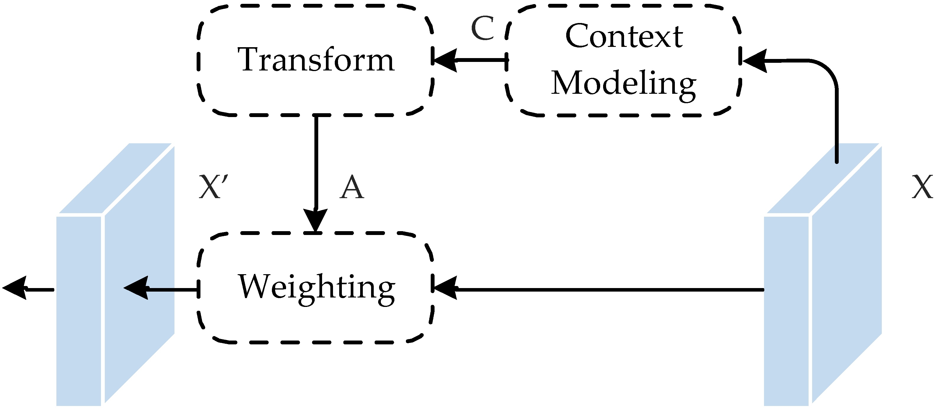
Previous studies have explored the importance of different levels of context and have made many improvements in semantic segmentation. However, these approaches tend to only focus on level-specific contextual relationships and do not harvest contextual information from a more holistic perspective. Consequently, these approaches are prone to suffer from a lack of contextual information (e.g., image-level context provides little improvement in identifying small targets). To this end, we aimed to seek an efficient and comprehensive approach that can model and transform contextual information.
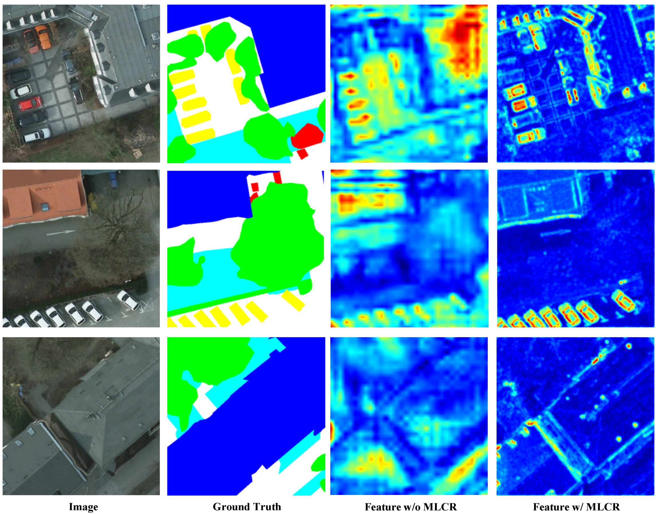
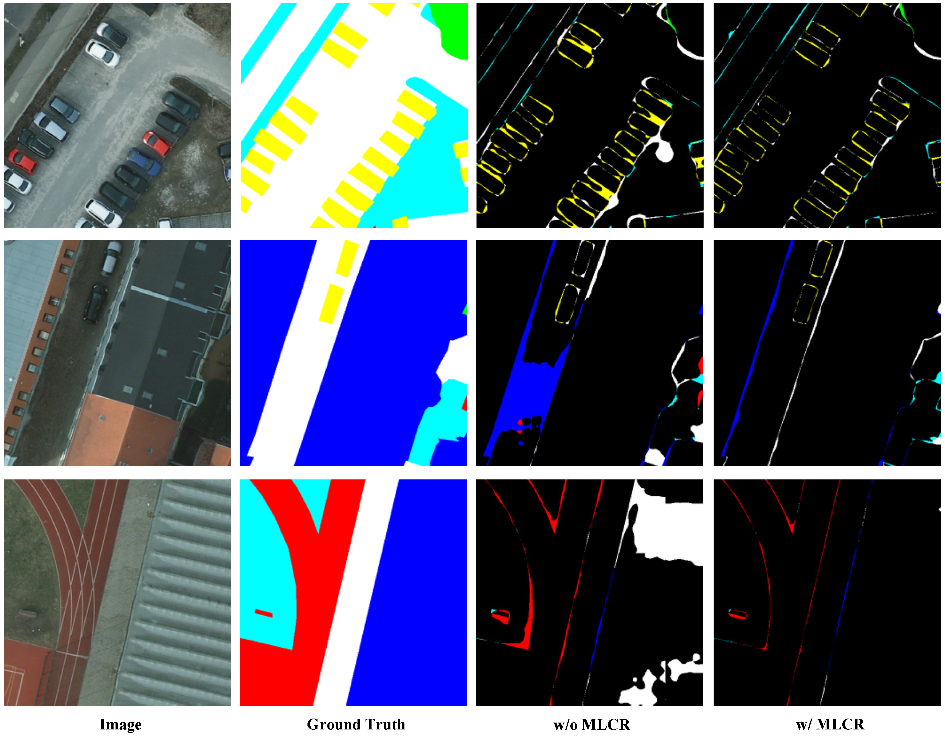
Initially, we directly integrated local-level, image-level, and semantic-level contextual attention matrices, which improved model performance but dramatically increased GPU memory usage and inference time. We realize that these three levels of context are not orthogonal. Moreover, concatenating the three levels of contextual attention matrices directly suffers from the redundancy of contextual information. Hence, we designed the EMCT module to transform the three levels of contextual relationships into a contextual attention matrix effectively and efficiently. The experimental results suggest that our proposed method has three advantages over other methods. First, our proposed MLCR module has made progress in quantitative experimental results, and ablation experimental results on the Potsdam test set reveal the effectiveness of our proposed module, thereby lifting the mIoU by 1.9% compared with the Baseline and outperforming other state-of-the-art models. Second, the computational cost of our proposed MLCR module is less than those of other contextual aggregation methods. Relative to DANet, MLCRNet reduces the number of parameters by 46% and the FLOPs by 78%. Lastly, from the qualitative experimental results, our MLCR module increases the consistency of intra-class segmentation and object boundary accuracy, as shown in the first row of Figure 10. MLCNet improves the quality of the car edges while solving the problem of misclassification of disturbed areas (e.g., areas between adjacent vehicles, areas obscured by building shadows). The second and third rows of Figure 10 show the power of MLCRNet to improve the intra-class consistency of large objects (e.g., buildings, roads, grassy areas, etc.). Nevertheless, for future practical applications, we need to continue to improve accuracy.

6. Conclusions

In this paper, we designed a novel MLCRNet that dynamically harvests contextual information from the semantic, image, and local perspectives for aerial image semantic segmentation. Concretely, we first integrated three levels of context, namely, local level, image level, and semantic level, to capture contextual information from multiple aspects adaptively. Next, an efficient fusion block is presented to address feature redundancy and improve the efficiency of our multi-level context. Finally, our model refines the feature map iteratively across FPN layers with MLCR. Extensive evaluations on Potsdam and Vaihingen challenging datasets demonstrate that our model can gather the multi-level contextual information efficiently, thereby enhancing the structure reasoning of the model.

Author Contributions

Z.H. and Q.Z. conceived of the presented idea and designed the study, respectively. Z.H. derived the models and performed the experiments. The manuscript was drafted by Z.H. with support from Q.Z. and G.Z. All authors discussed the results and contributed to the final manuscript. All authors have read and agreed to the published version of the manuscript.

Funding

This work was supported by the Natural Science Foundation of Shanghai (21ZR1421200), the National Nature Science Foundation of China (Grant Nos. 61731009 and 41301472), and the Science and Technology Commission of Shanghai Municipality (Grant Nos. 19511120600 and 18DZ2270800).

Institutional Review Board Statement

Not applicable.

Informed Consent Statement

Not applicable.

Data Availability Statement

The data and the code of this study are available from the corresponding author upon request.

Conflicts of Interest

The authors declare no conflict of interest.

Appendix A. Robustness Evaluation

Appendix A.1. Incorrect Labels and Rectification

During the early experiments, we noticed that two labels in Potsdam datasets (e.g., IDs: 4_12 and 6_7) were incorrect, with all pixels of labels 4_12 and some pixels of 6_7 (approximately 6000 pixels) inconsistent with the labels defined by the dataset publisher. We randomly selected three 512 × 512 patches in 4_12 (Figure A1). As shown in the second column, the original labels are mixed with noise, most likely because the dataset publisher failed to remove the original image channels after the tagging was completed.
After comparing the RGB channels of the incorrect labels with normals, we found that the RGB channels of the incorrect labels were shifted to varying degrees (offset ≤ 127). Therefore, we used the binarization operation to process the incorrect label:
G T k , i , j = { 255 , i f   G T k , i , j T 0 , o t e r w i s e
where G T R 3 × H × W is the original ground truth; G T R 3 × H × W is the fixed ground truth; and T is the threshold, which is set as T = 127 . We show the modified result in the third column of Figure A1. Next, we are to present the results of quantitative experiments on a training set that includes incorrect labels. Note that we have re-implemented the experiment with corrected labels and reported the results in the main text.
Figure A1. Error and binarization-corrected labels in the Potsdam datasets (best viewed when colored and zoomed in).
Remotesensing 14 01498 g0a1

Appendix A.2. Robustness Evaluation Results

We presented the experimental results before fixing the incorrect label to demonstrate the robustness of our proposed method. Table A1 shows that our method is less affected by the incorrect label than the other methods.
Table A1. Robustness evaluation results on the Potsdam test set.
ModelBackboneStridemIoU (%)Acc (%)F1
ISNet [32]ResNet5016×70.281.381.8
FCN [11]ResNet5016×71.581.982.8
OCRNet [29]ResNet5016×73.683.684.2
DepLabV3+ [15]ResNet5016×74.584.284.8
SCARF [31]ResNet5016×74.683.984.8
SFNet [17]ResNet5016×74.784.184.9
OursResNet5016×75.384.685.4

References

  1. Kang, Y.; Lu, Z.; Zhao, C.; Xu, Y.; Kim, J.-W.; Gallegos, A.J. InSAR monitoring of creeping landslides in mountainous regions: A case study in Eldorado National Forest, California. Remote Sens. Environ. 2021, 258, 112400. [Google Scholar] [CrossRef]
  2. Bianchi, F.M.; Grahn, J.; Eckerstorfer, M.; Malnes, E.; Vickers, H. Snow avalanche segmentation in SAR images with fully convolutional neural networks. IEEE J. Sel. Top. Appl. Earth Obs. Remote Sens. 2020, 14, 75–82. [Google Scholar] [CrossRef]
  3. Xu, F.; Somers, B. Unmixing-based Sentinel-2 downscaling for urban land cover mapping. ISPRS J. Photogramm. Remote Sens. 2021, 171, 133–154. [Google Scholar] [CrossRef]
  4. Luo, X.; Tong, X.; Pan, H. Integrating multiresolution and multitemporal Sentinel-2 imagery for land-cover mapping in the Xiongan New Area, China. IEEE Trans. Geosci. Remote Sens. 2021, 59, 1029–1040. [Google Scholar] [CrossRef]
  5. Azizi, A.; Abbaspour-Gilandeh, Y.; Vannier, E.; Dusséaux, R.; Mseri-Gundoshmian, T.; Moghaddam, H.A. Semantic segmentation: A modern approach for identifying soil clods in precision farming. Biosyst. Eng. 2020, 196, 172–182. [Google Scholar] [CrossRef]
  6. Anand, T.; Sinha, S.; Mandal, M.; Chamola, V.; Yu, F.R. AgriSegNet: Deep aerial semantic segmentation framework for iot-assisted precision agriculture. IEEE Sens. J. 2021, 21, 17581–17590. [Google Scholar] [CrossRef]
  7. Azimi, S.M.; Fischer, P.; Korner, M.; Reinartz, P. Aerial LaneNet: Lane-marking semantic segmentation in aerial imagery using wavelet-enhanced cost-sensitive symmetric fully convolutional neural networks. IEEE Trans. Geosci. Remote Sens. 2019, 57, 2920–2938. [Google Scholar] [CrossRef] [Green Version]
  8. Xu, Y.; Chen, H.; Du, C.; Li, J. MSACon: Mining spatial attention-based contextual information for road extraction. IEEE Trans. Geosci. Remote Sens. 2021, 60, 5604317. [Google Scholar] [CrossRef]
  9. Song, L.; Xia, M.; Jin, J.; Qian, M.; Zhang, Y. SUACDNet: Attentional change detection network based on siamese U-shaped structure. Int. J. Appl. Earth Obs. Geoinf. 2021, 105, 102597. [Google Scholar] [CrossRef]
  10. Krizhevsky, A.; Sutskever, I.; Hinton, G.E. ImageNet classification with deep convolutional neural networks. In Advances in Neural Information Processing Systems; Pereira, F., Burges, C.J.C., Bottou, L., Wein-berger, K.Q., Eds.; Curran Associates, Inc.: Red Hook, NY, USA, 2012; Volume 25. [Google Scholar]
  11. Long, J.; Shelhamer, E.; Darrell, T. Fully convolutional networks for semantic segmentation. In Proceedings of the IEEE Conference on Computer Vision and Pattern Recognition (CVPR), Boston, MA, USA, 7–12 June 2015; IEEE Computer Society: Los Alamitos, CA, USA, 2015; pp. 3431–3440. [Google Scholar]
  12. Girshick, R. Fast R-CNN. In Proceedings of the 2015 IEEE International Conference on Computer Vision (ICCV), Santiago, Chile, 7–13 December 2015; pp. 1440–1448. [Google Scholar] [CrossRef]
  13. Chen, L.-C.; Papandreou, G.; Kokkinos, I.; Murphy, K.; Yuille, A.L. DeepLab: Semantic image segmentation with deep convolutional nets, atrous convolution, and fully connected CRFs. IEEE Trans. Pattern Anal. Mach. Intell. 2018, 40, 834–848. [Google Scholar] [CrossRef] [Green Version]
  14. Chen, L.-C.; Papandreou, G.; Schroff, F.; Adam, H. Rethinking atrous convolution for semantic image segmentation. arXiv 2017, arXiv:1706.05587. [Google Scholar]
  15. Chen, L.-C.; Zhu, Y.; Papandreou, G.; Schroff, F.; Adam, H. Encoder-decoder with atrous separable convolution for semantic image segmentation. In Proceedings of the European Conference on Computer Vision (ECCV), Munich, Germany, 8–14 September 2018. [Google Scholar]
  16. He, K.; Zhang, X.; Ren, S.; Sun, J. Deep residual learning for image recognition. In Proceedings of the 2016 IEEE Conference on Computer Vision and Pattern Recognition (CVPR), Las Vegas, NV, USA, 27–30 June 2016; pp. 770–778. [Google Scholar]
  17. Li, X.; You, A.; Zhu, Z.; Zhao, H.; Yang, M.; Yang, K.; Tan, S.; Tong, Y. Semantic flow for fast and accurate scene parsing. In Proceedings of the Computer Vision—ECCV 2020, Glasgow, UK, 23–28 August 2020; Vedaldi, A., Bischof, H., Brox, T., Frahm, J.-M., Eds.; Springer International Publishing: Cham, Switzerland, 2020; pp. 775–793. [Google Scholar]
  18. Kirillov, A.; Girshick, R.; He, K.; Dollár, P. Panoptic feature pyramid networks. In Proceedings of the 2019 IEEE/CVF Conference on Computer Vision and Pattern Recognition (CVPR), Long Beach, CA, USA, 15–20 June 2019; pp. 6399–6408. [Google Scholar]
  19. Ronneberger, O.; Fischer, P.; Brox, T. U-Net: Convolutional networks for biomedical image seg-mentation. In Proceedings of the Medical Image Computing and Computer-Assisted Intervention—MICCAI 2015, Munich, Germany, 5–9 October 2015; Navab, N., Hornegger, J., Wells, W.M., Frangi, A.F., Eds.; Springer International Publishing: Cham, Switzerland, 2015; pp. 234–241. [Google Scholar]
  20. Lin, T.Y.; Dollár, P.; Girshick, R.; He, K.; Hariharan, B.; Belongie, S. Feature pyramid networks for object detection. In Proceedings of the 2017 IEEE Conference on Computer Vision and Pattern Recognition (CVPR), Honolulu, HI, USA, 21–26 July 2017; pp. 936–944. [Google Scholar] [CrossRef] [Green Version]
  21. Wang, X.; Girshick, R.; Gupta, A.; He, K. Non-local neural networks. In Proceedings of the 2017 IEEE Conference on Computer Vision and Pattern Recognition (CVPR), Honolulu, HI, USA, 21–26 July 2017. [Google Scholar]
  22. Fu, J.; Liu, J.; Tian, H.; Li, Y.; Bao, Y.; Fang, Z.; Lu, H. Dual attention network for scene segmentation. In Proceedings of the 2019 IEEE/CVF Conference on Computer Vision and Pattern Recognition (CVPR), Long Beach, CA, USA, 15–20 June 2019; pp. 3141–3149. [Google Scholar] [CrossRef] [Green Version]
  23. Hu, P.; Caba, F.; Wang, O.; Lin, Z.; Sclaroff, S.; Perazzi, F. Temporally distributed networks for fast video semantic segmentation. In Proceedings of the 2020 IEEE/CVF Conference on Computer Vision and Pattern Recognition (CVPR), Seattle, WA, USA, 13–19 June 2020; pp. 8815–8824. [Google Scholar]
  24. Zhang, H.; Wang, C.; Xie, J. Co-occurrent features in semantic segmentation. In Proceedings of the 2019 IEEE/CVF Conference on Computer Vision and Pattern Recognition (CVPR), Long Beach, CA, USA, 15–20 June 2019; pp. 548–557. [Google Scholar]
  25. Zhu, Z.; Xu, M.; Bai, S.; Huang, T.; Bai, X. Asymmetric non-local neural networks for semantic segmentation. In Proceedings of the 2019 IEEE/CVF International Conference on Computer Vision (ICCV), Seoul, Korea, 27 October–2 November 2019; pp. 593–602. [Google Scholar]
  26. Yan, L.; Huang, J.; Xie, H.; Wei, P.; Gao, Z. Efficient depth fusion transformer for aerial image semantic segmentation. Remote Sens. 2022, 14, 1294. [Google Scholar] [CrossRef]
  27. Yu, C.; Wang, J.; Gao, C.; Yu, G.; Shen, C.; Sang, N. Context prior for scene segmentation. In Proceedings of the 2020 IEEE/CVF Conference on Computer Vision and Pattern Recognition (CVPR), Seattle, WA, USA, 13–19 June 2020; pp. 12413–12422. [Google Scholar]
  28. Bello, I. LambdaNetworks: Modeling long-range interactions without attention. In Proceedings of the International Conference on Learning Representations, Vienna, Austria, 4 May 2021. [Google Scholar]
  29. Yuan, Y.; Chen, X.; Wang, J. Object-contextual representations for semantic segmentation. In Proceedings of the Computer Vision—ECCV 2020, Glasgow, UK, 23–28 August 2020; Vedaldi, A., Bischof, H., Brox, T., Frahm, J.-M., Eds.; Springer International Publishing: Cham, Switzerland, 2020; pp. 173–190. [Google Scholar]
  30. Zhang, F.; Chen, Y.; Li, Z.; Hong, Z.; Liu, J.; Ma, F.; Han, J.; Ding, E. ACFNet: Attentional class feature network for semantic segmentation. In Proceedings of the 2019 IEEE/CVF International Conference on Computer Vision (ICCV), Seoul, Korea, 27 October–2 November 2019; pp. 6797–6806. [Google Scholar]
  31. Ding, X.; Shen, C.; Che, Z.; Zeng, T.; Peng, Y. SCARF: A semantic constrained attention refinement network for semantic segmentation. In Proceedings of the 2021 IEEE/CVF International Conference on Computer Vision Workshops (ICCVW), Montreal, BC, Canada, 11–17 October 2021; pp. 3002–3011. [Google Scholar]
  32. Jin, Z.; Liu, B.; Chu, Q.; Yu, N. ISNet: Integrate image-level and semantic-level context for semantic segmentation. In Proceedings of the IEEE/CVF International Conference on Computer Vision, Montreal, BC, Canada, 11–17 October 2021. [Google Scholar]
  33. Niu, R.; Sun, X.; Tian, Y.; Diao, W.; Chen, K.; Fu, K. Hybrid multiple attention network for semantic segmentation in aerial images. IEEE Trans. Geosci. Remote Sens. 2021, 60, 5603018. [Google Scholar] [CrossRef]
  34. Shang, R.; Zhang, J.; Jiao, L.; Li, Y.; Marturi, N.; Stolkin, R. Multi-scale adaptive feature fusion network for semantic segmentation in remote sensing images. Remote Sens. 2020, 12, 872. [Google Scholar] [CrossRef] [Green Version]
  35. Zhang, J.; Lin, S.; Ding, L.; Bruzzone, L. Multi-scale context aggregation for semantic segmentation of remote sensing images. Remote Sens. 2020, 12, 701. [Google Scholar] [CrossRef] [Green Version]
  36. Xu, Z.; Zhang, W.; Zhang, T.; Li, J. Hrcnet: High-resolution context extraction net-work for semantic segmentation of remote sensing images. Remote Sens. 2020, 13, 71. [Google Scholar] [CrossRef]
  37. Fan, M.; Lai, S.; Huang, J.; Wei, X.; Chai, Z.; Luo, J.; Wei, X. Rethinking BiSeNet for real-time semantic segmentation. In Proceedings of the 2021 IEEE/CVF Conference on Computer Vision and Pattern Recognition (CVPR), Nashville, TN, USA, 20–25 June 2021; pp. 9711–9720. [Google Scholar]
  38. Wang, J.; Sun, K.; Cheng, T.; Jiang, B.; Deng, C.; Zhao, Y.; Liu, D.; Mu, Y.; Tan, M.; Wang, X.; et al. Deep high-resolution representation learning for visual recognition. IEEE Trans. Pattern Anal. Mach. Intell. 2021, 43, 3349–3364. [Google Scholar] [CrossRef] [Green Version]
  39. Hu, J.; Shen, L.; Sun, G. Squeeze-and-excitation networks. In Proceedings of the 2018 IEEE Conference on Computer Vision and Pattern Recognition (CVPR), Salt Lake City, UT, USA, 18–23 June 2018; pp. 7132–7141. [Google Scholar]
  40. Cao, Y.; Xu, J.; Lin, S.; Wei, F.; Hu, H. Gcnet: Non-local networks meet squeeze-excitation networks and beyond. In Proceedings of the 2019 IEEE/CVF International Conference on Computer Vision Workshop (ICCVW), Seoul, Korea, 27–28 October 2019; pp. 1971–1980. [Google Scholar] [CrossRef] [Green Version]
  41. Song, Q.; Li, J.; Li, C.; Guo, H.; Huang, R. Fully attentional network for semantic segmentation. arXiv 2021, arXiv:2112.04108. [Google Scholar]
  42. Li, R.; Zheng, S.; Zhang, C.; Duan, C.; Su, J.; Wang, L.; Atkinson, P.M. Multiattention network for semantic segmentation of fine-resolution remote sensing images. IEEE Trans. Geosci. Remote Sens. 2021, 60, 5607713. [Google Scholar] [CrossRef]
  43. Huang, L.; Yuan, Y.; Guo, J.; Zhang, C.; Chen, X.; Wang, J. Interlaced sparse self-attention for semantic segmentation. arXiv 2019, arXiv:1907.12273. [Google Scholar]
  44. Huang, Z.; Wang, X.; Wei, Y.; Huang, L.; Shi, H.; Liu, W.; Huang, T.S. CCNet: Criss-cross attention for semantic segmentation. IEEE Trans. Pattern Anal. Mach. Intell. 2020, 1, 9133304. [Google Scholar] [CrossRef]
  45. Zhao, H.; Shi, J.; Qi, X.; Wang, X.; Jia, J. Pyramid scene parsing network. In Proceedings of the 2017 IEEE Conference on Computer Vision and Pattern Recognition (CVPR), Honolulu, HI, USA, 21–26 July 2017; pp. 6230–6239. [Google Scholar] [CrossRef] [Green Version]
  46. Zhang, Q.; Yang, G.; Zhang, G. Collaborative network for super-resolution and semantic segmentation of remote sensing images. IEEE Trans. Geosci. Remote Sens. 2021, 60, 4404512. [Google Scholar] [CrossRef]
  47. Saha, S.; Mou, L.; Qiu, C.; Zhu, X.X.; Bovolo, F.; Bruzzone, L. Unsupervised deep joint segmentation of multitemporal high-resolution images. IEEE Trans. Geosci. Remote Sens. 2020, 58, 8780–8792. [Google Scholar] [CrossRef]
  48. Du, S.; Du, S.; Liu, B.; Zhang, X. Incorporating DeepLabv3+ and object-based image analysis for semantic segmentation of very high resolution remote sensing images. Int. J. Digit. Earth 2020, 14, 357–378. [Google Scholar] [CrossRef]
  49. Yang, G.; Zhang, Q.; Zhang, G. EANet: Edge-aware network for the extraction of buildings from aerial images. Remote Sens. 2020, 12, 2161. [Google Scholar] [CrossRef]
  50. He, K.; Zhang, X.; Ren, S.; Sun, J. Identity mappings in deep residual networks. In Proceedings of the Computer Vision—ECCV 2016, Amsterdam, The Netherlands, 11–14 October 2016; Leibe, B., Matas, J., Sebe, N., Welling, M., Eds.; Springer International Publishing: Cham, Switzerland, 2016; pp. 630–645. [Google Scholar]
  51. Xie, S.; Girshick, R.; Dollár, P.; Tu, Z.; He, K. Aggregated Residual Transformations for Deep Neural Networks. In Proceedings of the 2017 IEEE Conference on Computer Vision and Pattern Recognition (CVPR), Honolulu, HI, USA, 21–26 July 2017; pp. 5987–5995. [Google Scholar] [CrossRef] [Green Version]
  52. ISPRS 2D Semantic Labeling Contest. 2016. Available online: https://www2.isprs.org/commissions/comm2/wg4/benchmark/2d-sem-label-potsdam/ (accessed on 15 December 2020).
  53. Russakovsky, O.; Deng, J.; Su, H.; Krause, J.; Satheesh, S.; Ma, S.; Huang, Z.; Karpathy, A.; Khosla, A.; Bernstein, M.; et al. ImageNet large scale visual recognition challenge. Int. J. Comput. Vis. 2015, 115, 211–252. [Google Scholar] [CrossRef] [Green Version]
  54. He, K.; Zhang, X.; Ren, S.; Sun, J. Delving deep into rectifiers: Surpassing human-level performance on imagenet classification. In Proceedings of the International Conference on Computer Vision (CVPR), Las Condes, Chile, 11–18 December 2015; pp. 1026–1034. [Google Scholar]
  55. Ioffe, S.; Szegedy, C. Batch normalization: Accelerating deep network training by reducing internal covariate shift. In Proceedings of the 32nd International Conference on International Conference on Machine Learning, Lille, France, 7–9 July 2015; Volume 37, pp. 448–456. [Google Scholar]
  56. Bulo, S.R.; Porzi, L.; Kontschieder, P. In-place activated batchnorm for memory-optimized training of DNNs. In Proceedings of the 2018 IEEE/CVF Conference on Computer Vision and Pattern Recognition, Salt Lake City, UT, USA, 18–23 June 2018; pp. 5639–5647. [Google Scholar]
  57. Lee, C.-Y.; Xie, S.; Gallagher, P.; Zhang, Z.; Tu, Z. Deeply-supervised nets. In Proceedings of the Eighteenth International Conference on Artificial Intelligence and Statistics, San Diego, CA, USA, 9–12 May 2015; Lebanon, G., Vishwanathan, S.V.N., Eds.; PMLR: San Diego, CA, USA, 2015; Volume 38, pp. 562–570. [Google Scholar]
  58. Paszke, A.; Gross, S.; Massa, F.; Lerer, A.; Bradbury, J.; Chanan, G.; Killeen, T.; Lin, Z.; Gimelshein, N.; Antiga, L.; et al. PyTorch: An imperative style, high-performance deep learning library. In Proceedings of the Advances in Neural Information Processing Systems 32: Annual Conference on Neural Information Processing Systems 2019, NeurIPS 2019, Vancouver, BC, Canada, 8–14 December 2019; Wallach, H.M., Larochelle, H., Beygelzimer, A., d’Alché-Buc, F., Fox, E.B., Garnett, R., Eds.; Curran Associates, Inc.: Red Hook, NY, USA, 2019; pp. 8024–8035. [Google Scholar]
  59. Oktay, O.; Schlemper, J.; Folgoc, L.L.; Lee, M.C.H.; Heinrich, M.P.; Misawa, K.; Mori, K.; McDonagh, S.G.; Hammerla, N.Y.; Kainz, B.; et al. Attention U-Net: Learning where to look for the pancreas. arXiv 2018, arXiv:1804.03999. [Google Scholar]
Figure 1. General contextual refinement framework.
Remotesensing 14 01498 g001
Figure 2. Local-level context module.
Remotesensing 14 01498 g002
Figure 3. The multi-level context transform (MCT) module.
Remotesensing 14 01498 g003
Figure 4. The efficient multi-level context transform (EMCT) module. The image-level contextual information C I is first embedded into semantic-level contextual information C S , then we further fuse them with local contextual information matrix C L by matrix multiplication to generate multi-level contextual attention matrix A M L .
Remotesensing 14 01498 g004
Figure 5. MLCR module.
Remotesensing 14 01498 g005
Figure 6. Overview of the proposed MLCRNet.
Remotesensing 14 01498 g006
Figure 7. Visualization of features. Our module enhances the representation of more structural features.
Remotesensing 14 01498 g007
Figure 8. Qualitative comparisons against the Baseline on the Potsdam test set. We marked the improved regions with red dashed boxes (best viewed when colored and zoomed in).
Remotesensing 14 01498 g008
Figure 9. Qualitative comparisons between our method and Baseline on Vaihingen test set. We marked the improved regions with red dashed boxes (best viewed when colored and zoomed in).
Remotesensing 14 01498 g009
Figure 10. Qualitative comparison in terms of prediction errors on Potsdam test set, where correctly predicted pixels are shown with a black background and incorrectly predicted pixels are colored using the prediction results (best viewed when colored and zoomed in).
Remotesensing 14 01498 g010
Table 1. Ablation results for MLCR module to different insert positions on Potsdam test set.
Method321mIoU (%)∆α (%)
Baseline 74.1
MLCR 74.8 0.7 ↑
MLCR 75.0 0.9 ↑
MLCR 75.4 1.3 ↑
MLCR 75.7 1.6 ↑
MLCR76.0 1.9 ↑
Table 2. Ablation studies of different level context on Potsdam test set.
MethodSILmIoU (%)∆α (%)
Baseline74.1
75.3 1.2 ↑
75.4 1.3 ↑
75.0 0.9 ↑
75.6 1.5 ↑
75.5 1.4 ↑
75.6 1.5 ↑
76.0 1.9 ↑
Table 3. Ablation study on kernel size k in local-level context module.
MethodmIoU (%)FLOPs (G)
k = 175.542.7
k = 376.043.3
k = 575.844.3
k = 775.845.9
Table 4. Ablation study on computation cost.
MethodMemory (Mb)Parameter (M)FLOPs (G)FPSmIoU (%)
Baseline915 25.2 42.7 90.3 74.1
MCT1170 (+255)27.3 (+2.1)50.7 (+8.0)63.6 (−26.7)75.8 (+1.7)
Efficient MCT917 (+2)25.7 (+0.5)43.3 (+0.6)80.0 (−10.3)76.0 (+1.9)
Table 5. Quantitative comparisons with state-of-the-arts on Potsdam test set.
ModelBackboneStridemIoU (%)Acc (%)F1Parameter (M)FLOPs (G)
FCN [11]ResNet5016×72.583.0 83.532.9 33.7
OCRNet [29]ResNet5016×73.984.0 84.439.0 47.6
CCNet [44]ResNet5016×74.184.1 84.647.4 57.4
ISANet [43]ResNet5016×74.584.5 84.840.0 49.5
PSPNet [45]ResNet5016×74.584.2 84.846.6 52.0
ACFNet [30]ResNet5016×74.784.3 84.930.1 39.3
DANet [22]ResNet5016×74.984.4 85.147.4 198.1
DepLabV3+ [15]ResNet5016×75.184.7 85.140.3 69.3
MANet [42]ResNet5016×75.284.7 85.233.5 49.6
AttUNet [59]ResNet5016×75.384.6 85.396.5 207.8
SFNet [17]ResNet5016×75.4 84.9 85.430.6 100.1
ISNet [32]ResNet5016×75.785.0 85.644.5 58.8
SCARF [31]ResNet5016×75.785.3 85.625.9 45.0
OursResNet5016×76.085.2 85.825.7 43.3
Table 6. Per-class results (mean intersection over union) on the Potsdam test set.
ModelImp.surBuildingLow.vegTreeCarCluttermIoU(%)
FCN [11]79.8 90.3 70.6 72.6 72.2 49.8 72.5
OCRNet [29]80.9 90.9 71.6 73.5 74.7 51.9 73.9
CCNet [44]81.1 91.5 71.9 73.3 75.6 51.3 74.1
ISANet [43]81.2 91.5 72.4 74.1 74.7 52.8 74.5
PSPNet [45]81.4 91.3 72.1 74.1 75.4 52.5 74.5
ACFNet [30]81.3 91.4 71.5 73.4 79.4 51.0 74.7
DANet [22]81.7 91.5 72.0 74.4 76.4 53.2 74.9
DepLabV3+ [15]81.5 91.4 72.0 73.1 80.9 51.4 75.1
MANet [42]81.6 91.1 72.2 73.8 81.7 50.6 75.2
AttUNet [59]81.6 91.3 71.9 73.1 81.4 52.3 75.3
SFNet [17]81.9 91.5 72.5 73.7 81.0 51.8 75.4
ISNet [32]82.1 91.7 72.7 74.3 81.1 52.1 75.7
SCARF [31]82.1 91.5 72.8 74.1 81.4 52.1 75.7
Ours82.3 91.4 73.1 73.7 81.6 53.7 76.0
Table 7. Quantitative comparisons with state-of-the-arts on Vaihingen test set.
ModelBackboneStridemIoU (%)Acc (%)F1
FCN [11]ResNet5016×64.6 74.7 77.1
CCNet [44]ResNet5016×65.5 75.2 77.7
OCRNet [29]ResNet5016×66.3 76.5 78.6
ISNet [32]ResNet5016×66.4 76.7 78.6
ISANet [43]ResNet5016×66.6 76.4 78.7
PSPNet [45]ResNet5016×66.6 76.0 78.6
ACFNet [30]ResNet5016×66.7 76.4 78.7
DANet [22]ResNet5016×66.8 76.4 78.8
DepLabV3+ [15]ResNet5016×66.9 76.4 78.8
MANet [42]ResNet5016×66.9 76.2 78.8
AttUNet [59]ResNet5016×67.1 76.4 79.0
OursResNet5016×68.1 77.5 79.8
Table 8. Per-class results (mean intersection over union) on the Vaihingen test set.
ModelImp.surBuildingsLow.vegTreeCarCluttermIoU (%)
FCN [11]78.9 86.1 63.8 72.8 49.9 36.0 64.6
CCNet [44]80.1 86.7 65.0 73.5 52.5 35.3 65.5
OCRNet [29]79.6 86.5 64.6 73.5 54.1 39.4 66.3
ISNet [32]79.8 86.1 63.8 72.9 58.8 36.9 66.4
ACFNet [30]80.6 87.1 65.2 74.1 57.8 35.3 66.7
DANet [22]80.1 86.4 65.3 73.8 59.4 36.0 66.8
DepLabV3+ [15]80.4 86.5 64.3 73.7 61.3 35.2 66.9
MANet [42]80.3 86.5 64.1 73.5 63.4 33.7 66.9
AttUNet [59]80.4 86.6 64.3 73.7 63.2 34.4 67.1
Ours81.3 87.2 65.4 74.3 64.4 36.1 68.1
Publisher’s Note: MDPI stays neutral with regard to jurisdictional claims in published maps and institutional affiliations.

