Forecast of the Global TEC by Nearest Neighbour Technique

Abstract

We propose a method for Global Ionospheric Maps of Total Electron Content forecasting using the Nearest Neighbour method. The assumption is that in a database of global ionosphere maps spanning more than two solar cycles, one can select a set of past observations that have similar geomagnetic conditions to those of the current map. The assumption is that the current ionospheric condition can be expressed by a linear combination of conditions seen in the past. The average of these maps leads to common geomagnetic components being preserved and those not shared by several maps being reduced. The method is based on searching the historical database for the dates of the maps closest to the current map and using as a prediction the maps in the database that correspond to time shifts on the prediction horizons. In contrast to other methods of machine learning, the implementation only requires a distance computation and does not need a previous step of model training and adjustment for each prediction horizon. It also provides confidence intervals for the forecast. The method has been analyzed for two full years (2015 and 2018), for selected days of 2015 and 2018, i.e., two storm days and two non-storm days and the performance of the system has been compared with CODE (24- and 48-h forecast horizons).

1. Introduction

The variations in electron density and, correspondingly in its line-of-sight integral, the vertical total ionospheric electron content (TEC), affect satellite telecommunication services and Global Navigation Satellite Systems (GNSS) due to the effect these fluctuations have on radio wave propagation. The TEC variations induce changes that affect the transmission quality either as reduced transmission rate or positioning errors. This justifies the importance of monitoring and predicting global TEC maps, as the knowledge of the spatial distribution of TEC would allow corrections to be made. The TEC measurement consists of the total number of electrons integrated along a 1 m² cross-section tube, using as a unit the TECU defined as = 10¹⁶ electrons/m². The prediction of Global Ionospheric Maps (GIM) at different horizons is important because the ionospheric delay is main limiting factor in high-accuracy positioning. These predictions may allow achieving sub-meter accuracy for mass-market single-frequency receivers [1]. In this paper we propose a method for Global Ionospheric Maps of Total Electron Content forecasting using the nearest neighbour method which we denote as NNGIM.

1.1. Issues Related to Previous Work in TEC Map Prediction

The difficulty in predicting TEC maps of the ionosphere stems from the fact that the quality of the prediction depends on geomagnetic activity, season, geographical location, ionospheric structures, such as equatorial ionization anomaly (EIA), and storm-enhanced density (SED). Besides, the sparsity in the geographical distribution of stations leads to problems related to interpolation in regions not covered by these stations. Added to the problem of variability and dependence on external factors, the prediction of GIM maps by machine learning techniques is affected by the need for machine learning techniques to infer prediction rules from examples. This means that the database to train the system has to be rich enough to represent most of the combinations of effects acting on the ionosphere. One intrinsic limitation of machine learning-based systems is the availability of a database that sufficiently covers the multiple forms of phenomena that can occur. In the works cited below, most of the prediction proposals are made using databases covering at most one solar cycle. In this work, we will be using UPC-IonSAT’s database (for more information about the IonSAT group, i.e., ionospheric determination and navigation based on satellite and terrestrial systems group see [2]), which covers more than two solar cycles. It is important to highlight the importance of having more than one solar cycle to infer the structure and parameters of the forecasting system. Within the long-term solar cycle periodicity, there is large variability. As an example analyzed in this paper, we can mention two dates when storms occur. For instance, the Saint Patrick storm of 17 March 2015 (maximum of solar cycle C23) and the storm of 25–26 August 2018 (minimum of solar cycle C23). These are dates in different phases of the solar cycle, in which we have high solar and geomagnetic activity superimposed on different basal levels of ionization. The 

Table 1. Hourly Kp for the 17 March 2015.

Hour	00–03 h	03–06 h	06–09 h	09–12 h	12–15 h	15-18 h	18–21 h	21–00 h
Kp (17 March)	2	5	6	6	8	8	7	8

and

Table 2. Hourly Kp for the 25–26 August 2018.

Hour	00–03 h	03–06 h	06–09 h	09–12 h	12–15 h	15–18 h	18–21 h	21–00 h
Kp (25 August)	1	1	2	2	3	2	4	4
Kp (26 August)	5	7	7	5	5	6	5	3

, summarise the hourly Kp values on these days. In these two days, the activity in terms of Kp values and magnitude of the flares is similar. Therefore, within the periodicity associated with the solar cycles and the season of the year, there is a high variability that makes it difficult to infer prediction rules. This high variability, in addition to the baseline levels of activity due to the periodicity components, justifies the need for a long enough database.

The need for a database that sufficiently covers the variability of GIMs presents significant technical problems from the point of view of prediction algorithms. In the case of two solar cycles, with maps at a rate of one every 15 min, the resulting database consists of more than one million maps. The use of databases of this size makes the hardware requirements demanding, and the computational time requirements to perform topology and parameter tuning of the machine learning system are substantial.

To address the above mentioned problem, i.e., of training a machine learning system for forecasting the GIMs, making, there are two approaches.

Local approach: In this case, a specific subset of the database is constructed from the current observation. An example is [3], in which maps immediately before the current map are used, and the forecasting method is based on these maps and the associated tangent spaces, which are linearly combined to generate the predicted maps. This approach assumes that the change in the maps has inertia that determines the future evolution. In [4], they apply a similar idea to calculate the autoregression coefficients that predict the values of the spherical harmonics that allow the GIMs to be reconstructed. Another approach is the one followed in this article, in which prediction is made based on past examples that have a small distance to the current observation. This approach assumes that conditions similar to the one observed in the current map have occurred in the near past and that the temporal evolution of the current map can be inferred from the evolutions seen in the previous history. A noteworthy aspect of the local approximation is that increasing the number of prediction horizons does not lead to a significant increase in computation time, as most of the computation time comes from determining the coefficients in a window that spans a limited amount of time.

Global approach: In this case, the prediction model uses all the historical GIMs. One consequence of this is that to make a reliable prediction, the  model has to be estimated from a sufficiently rich set of examples. This leads to problems of implementation. For support vector machines, this approach is infeasible, since it is necessary to create the gram matrix, which is the square of the number of examples, and it must be kept in memory. In the case of deep learning [5], the training has to be carried out in graphical processing units (GPU), which have limited memory.

Another significant limitation in the approach using deep learning and similar methods is that either a completely new model or a more complicated topology has to be trained when increasing the number of prediction horizons. In contrast, the method we propose, the nearest neighbour GIM algorithm (NNGIM), is based on finding the nearest set of maps, increasing or changing the values of the horizons has minimal repercussions on the execution time.

A natural model for forecasting the GIM maps that has been used in the literature (see Section 1.2) is the long short term memory (LSTM) [5] architecture. A very significant limitation of the LSTM architectures is that they consist of units that have saturating nonlinearities, such as hyperbolic tangent and sigmoid. Since the GIM statistics are long tail (see the last section of [3]), the units work much of the time in saturation and cannot model large amplitudes. For a complete explanation see Section 4.4. One consequence is that precisely the regions of interest where there are large TEC gradients cannot be modelled correctly by these units, as the gradient is zero due to the saturation of the nonlinearities. The complexity of using Deep Learning based methods was one of the motivations for seeking a more simple approach to the problem.

1.2. Approaches and Limitations to the GIM Forecast

We will now discuss some antecedents to set the NNGIM in context. The features and limitations of other GIM prediction methods will allow us to justify NNGIM design decisions. This section will also serve to highlight the limitations of the global approach to forecasting.

Global approach: A first approach to the problem of predicting TEC maps consists of predicting TEC values for specific stations, thus obtaining a local description of the TEC distribution. This is the case of [6], where they predict the TEC over China using a variant of the LSTM type networks (ED-LSTM). This type of method differs from ours in the sense that the prediction is done at the station level and there is no interpolation process. One point to note is the use of data from one solar cycle (January 2006 to April 2018). The authors use training data from 2006 to 2016, validation between January 2017 and April 2018. To avoid the problem of the solar cycle-dependent baseline TEC level, and to adapt the data to the structure of the LSTM grids, the authors normalise the data. This assumes that the variations around the baseline TEC value are similar between different times of the solar cycle. One problem related to their approach is that the neural network units they apply have saturation-type non-linearities, which has as a consequence that for extreme values, the units work on saturation (i.e., the gradients are null, and the extreme value is set to the limit of the saturation function). Note that the statistics of the TEC distribution is Leptokurtic, i.e., long tail, which means that extreme values are much more common than expected in the case of a Gaussian or Exponential distribution. On the other hand, an advantage of the type of neural network they employ is that it allows the use of external data naturally in the architecture (solar flux and geomagnetic activity data). In addition to the LSTM architecture (ED-LSTM), the authors explore other architectures and provide a performance hierarchy. The forecast horizons are 2-h, 3-h, and 4-h, using as input a window of past samples between one day and three days. An important lesson from this work is that the inertia hypothesis, in the sense that the temporal evolution of the TEC follows a trajectory specified by the near past, leads to a prediction barrier at a horizon of a few hours. This limit on the prediction horizon under these conditions was also found in [3].

Another paper working on the prediction of TEC values using a network of local stations in Turkey is [7]. Unlike the present paper, which deals with stations distributed all over the globe, the authors use five stations, all located in the mid-latitude region. The training implementation uses inputs corresponding to the current TEC value, together with measurements affecting the evolution of ionization, such as Kp, solar flux (F10.7 cm), magnetic field (Bx, By and Bz) and proton density, and EUV radiation in two bands. The neural network they use is based on LSTM structures, which suffer from the above-mentioned drawback, i.e., the input signal has a Leptokurtic statistic. In other words, outliers are common (for instance Figures 5 to 7 of the article [6]), while the prediction mechanism is based on LSTM units that saturate at high levels of any of the inputs. This means that in situations of high ionization variations, this approach does not allow the prediction model to learn from these variations. Another aspect that concerns us in the current implementation is the robustness of the prediction system with respect to the measurements. The fact of using heterogeneous measurements as input to the network makes the prediction susceptible to events of loss of some type of measurement.

A similar paper is [8] that performs the map prediction on a single meridian, 120 degrees, in a range of latitudes between 80 degrees north and 80 degrees south, (in contrast to our case, where we perform a global prediction). They use as input to the system a history of past measurements of daily TEC sampled at 2-h intervals, together with the mean value of the solar flux. An interesting feature of this work is that the use of external information (kp and Dst) had a different influence depending on the phase of the solar cycle. Another limitation, which is common to other applications using neural networks, is the partitioning between train, test and validation. In this case, for the validation partition, the years 2015 and 2018 were used, which correspond to the time after the peak of activity and when the activity decreases. Since the statistics of the TEC variation and the external information used are different according to the phase of the solar cycle, this partition introduces a bias in the architecture and parameters selected for the predictor. Moreover, the use of sigmoid/hyperbolic nonlinearities in LSTM/MLP prediction methods leads to the limitations discussed in Section 4.4.

An article reporting a related architecture is [9]. Unlike the previous case, the objective was to predict global TEC maps, with a resolution of 5 by 2.5 degrees in longitude and latitude. The temporal resolution was 2 h. To solve the diurnal cyclicity problem, they use a solar centred reference frame. The authors propose the prediction of global maps with prediction horizons increasing in two-hour steps up to 48 h. The input data were the maps for the three immediately preceding days. The type of architecture they propose is based on a sequence to sequence, in which CNN-type networks are combined with memory networks, either LSTM or gated recurrent units (GRU), both with saturating nonlinearities. The authors report that prediction at intervals longer than 24 h did not achieve good results; in fact, in the 24-h prediction, they obtain a result that improves the cyclic prediction by only 6%. The study was conducted using the data from 1 January 2014 to 31 December 2016. Note also, that the use of LSTM or GRU also suffers from the limitation that the observations are leptokurtic, which means that the nolinearities work in saturation for extreme values.

In [10] the authors propose a system based on the use of two LSTM layers followed by a fully connected dense layer for the prediction of the global TEC maps. Unlike the previous cases, the prediction is performed directly on the spherical harmonic (SH) used to build the GIMs. In this approach, in addition to using the information in the recent past (24 h) regarding the SH, they also use external information that helps to make the prediction, such as the solar extreme ultraviolet (EUV) flux, the hour of the day, and disturbance storm time (Dst) index. The prediction horizon is set to 1 h and 2 h. It is interesting to note that the prediction has an error with respect to frozen maps (defined as persistence, i.e., $\widehat{M}a{p}_{frozen}(t+\tau )=Map\left(t\right)$) of 60% at one hour and 63% at two hours. Note that (although the experiment is not totally comparable) this gain is similar to the obtained by the frozen cyclic approach vs. the persistence hypothesis, in Section 2.5 of the current paper. As a test base, the intervals before and after the interval used for the training base were used. That is, for the training base the interval: 1 January 2015 to 26 May 2016 and for the test base the intervals 19 October to 31 December 2014 and 27 May to 31 December 2016, thus ensuring a similarity between the training and test conditions.

The methodology of the above-mentioned works is correct from the point of view of deep learning type network design, however, despite the correctness, it reflects the limitations of this type of technique. These limitations are typical of the general approach to the TEC prediction problem using deep learning and do not indicate a misuse of the technique by the authors. The limitations of Deep Learning are the need to process the input data such as normalisation or de-trending of the TEC, the difficulty of performing a test under train-like conditions, the fact that some networks require saturating nonlinearities that are not fit for long-tail input distributions, and the limitations for predictions at horizons greater than 24 h.

A different approach to the GIMs prediction problem is the one proposed by [11], employing GANs (Generalized Adversarial Networks), which consists of a generative method, with a training criterion based on generating maps that compete with a system that generates impostors. It is a method that, by observing the current GIM map, generates the future one. Unlike most prediction systems, it does not depend on a previous history of GIM measurements, so it is robust to loss/reinitialization of the GIM data source. Like our method, it implicitly assumes that the external conditions that determine the evolution of the maps are included in the current measurement. However, an important limitation of this method is that the quality depends on the data used for training and validation. In the case of this publication this limitation is crucial, because the partition that was performed to train the method ((1) a training data set (2001–2011), (2) a validation data set (2012), and (3) a test data set (2013–2017)) makes that the criteria to determine the characteristics of the experiment given by the year of validation, induce a bias that makes the behavior of the predictions on unseen data depend on the accidental conditions of this partition and the peculiarities of the chosen cycle. This method does not have the limitations of the above mentioned methods in the sense that it does not use nonlinearities with saturation, and does not depend on additional measures to the GIM, which makes it robust to data loss.

Local approach: This approach uses information from recent past to estimate the parameters of the prediction model.

In [4], the authors describe a system based on autoregressive models, with coefficients computed from a history covering the previous 30 days. The prediction is made on the SH coefficients, which allow the GIM to be reconstructed. By estimating the model locally, they can adapt the system to short-term climatology. This allows them to test the model at different times of the solar cycle, without the need for special partitioning of the database, as is done in the case of deep learning. The performance of the model is tested against CODE, IGS products, and TEC measurements via JASON. The prediction result is different depending on the activity at the time, with worse results at times of high activity. One result is that the RMSE error of prediction during a low activity period was 1.5 TECUs at 24 h. In [12] the authors use autoregressive moving average (ARMA) for vertical TEC (VTEC) prediction for stations in Northern Europe. In this article, they use information related to the analysis in wavelets to establish the prediction at 1, 2, and 3-h horizons, calculating the ARMA coefficients from the last 7 days. The TEC profiles follow a daily pattern, so an ARMA-type method is suitable for modeling the cyclicities.

In [1], the authors propose a method for the prediction of GIMs with horizons of up to 2 days. It is based on a method that predicts the coefficients of the discrete cosine transform (DCT) by an autoregressive method. The autoregressive coefficients are calculated locally using information from the last week’s maps. From the predicted DCT coefficients, the map at the horizon of interest is computed. By calculating the coefficients using a recent past and using the maps of the previous 24 h for the prediction, the system can adapt to the current weather conditions. The results were validated with JASON measurements.

In [3] a prediction system is proposed based on an autoregressive model of the maps of the last 24 h, updated using only recent observations. The forecast also uses the components of the tangent spaces associated with each of the previous maps. The forecast horizons range from half an hour to 24 h. The tangent space information allows an increase in the information on the possible trajectory and deformation of the map over time, and in some way to reflect how the ionospheric climatology changes the shape of the high ionization regions. One feature related to the comparison with other methods is the percentage improvement of the prediction method compared to a frozen reference in a sun-fixed reference frame. The reference will be the prediction error of keeping the map frozen (see Section 2.5 for more information). As shown in

Table 3. Forecast vs. frozen (% RMSE) for the tangent space.

Horizon:	1/2 h	1 h	2 h	3 h	6 h	24 h
Forcast vs. Frozen:	84.99%	77.65%	71.35%	69.34%	87.23%	95.76%

, the prediction performance has a concave profile. The performance is computed using the recent past, and with autoregressive model coefficients calculated with recent values as well. The best prediction compared to frozen is at a 3-h horizon, increasing thereafter. At 24 h, the improvement is only 5%, which is in line with methods based on deep learning. This leads us to think that there is a certain horizon barrier in terms of prediction using the recent past as input.

The analysis of the previous approaches leads us to the conclusion that the information immediately prior to the current map does not allow reliable predictions of GIM maps at horizons longer than a few hours. They also indicate the limitations and difficulties of training prediction models, and the complexity of the models and partitions of the database.

This leads us to look for a different approach, in which the prediction is made by searching for situations similar to the current one in a sufficiently large database. A by-product of this approach is that it allows the creation of confidence margins of the forecast in a natural way (see Section 4.1).

2. Materials and Methods

2.1. UPC-IonSAT Real-Time Global Ionospheric Maps and Data Preprocessing

The GIMs are generated from data gathered from several hundred worldwide GNSS stations. This data stream is obtained through the protocol used by the RT IGS working group and the data processing is performed using the UPC-IonSAT ionosphere model.

The streaming protocol referred to as “Networked Transport of Radio Technical Commission for Maritime Services (RTCM) via Internet Protocol” (NTRIP), was developed by the German Federal Agency for Cartography and Geodesy (BKG), enables the streaming of the observation data from the worldwide permanent GNSS receivers [13].

The UPC-IonSAT’s RT TOMographic IONosphere Model (RT-TOMION) is a 4D (3D+time) model of the global state of the ionosphere, focused on RT estimation of TEC, mainly based on GPS dual-frequency measurements with the hybrid geodetic and tomographic ionospheric model, and robust to various types of deterioration. This model is the extension of the Tomographic Ionospheric Model (TOMION) developed by UPC in the 1990s and has been employed for UPC RT/near-RT ionosphere service of IGS since 2011 [14,15,16,17,18].

Additionally, the VTEC interpolation techniques of the UPC RT- TOMION model are performed either by spherical harmonics or Kriging [16] so to fill the gaps where data is lacking. In addition, the most recent maps are interpolated by means of the ADDGIM algorithm presented in [19]. For more details of the processing and interpolation of the GIMs, see [19].

2.2. The NNGIM Forecasting Algorithm

In this section, we will describe the Nearest Neighbour GIM (NNGIM) algorithm. This algorithm consists of searching for the N maps closest (in Euclidean metric) to the current one in the database of past maps (more than one solar cycle). Then, from these maps, the GIMs with an offset equal to the prediction horizon are retrieved and averaged.

The assumption underlying the NNGIM algorithm is that in a database that encompasses more than one solar cycle, a small number of maps with the property of being the closest in Euclidean distance to the current one can be found, and that have ionosphere conditions in common with the current one, might characterize the maps at a time shift equal to the forecast horizon. Although each ionosphere condition is unique, it is assumed that in the past there have been conditions with a similar composition of external features and that the average of all of them will reflect the specific features of the current one. The set of similar maps therefore take into account the cyclical aspects that influence the overall distribution of TEC along with the various external influences. That is, if we select a set of future map values closer to the current one when averaging, common values in subsets of the future maps will be retained, while non-common conditions will be attenuated. Note that the idea behind the assumption is that there will be subsets of maps representing similar ionospheric conditions, and the overall composition of these parts will allow us to approximate previously unseen situations. We assume that these previously unseen situations are composed of subgroups that characterize part of the previous conditions common to the current situation.

The UPC-IonSat GIMs database, which spans over two solar cycles and consists of more than ${10}^6$ maps, was used to implement the method (see [19] for details).

In the algorithm diagram, Algorithm 1, we present the summary of the NNGIM algorithm. A detailed explanation of the algorithm is given below, also defining the variables involved.

The input of the algorithm consists of a database spanning more than two solar cycles ($D{b}_{AllMaps}$). Note that for consistency in the computation of the distance between maps at different moments, the database and the current map are transformed to sun-fixed geomagnetic coordinates. After the forecast, the inverse transform is performed.

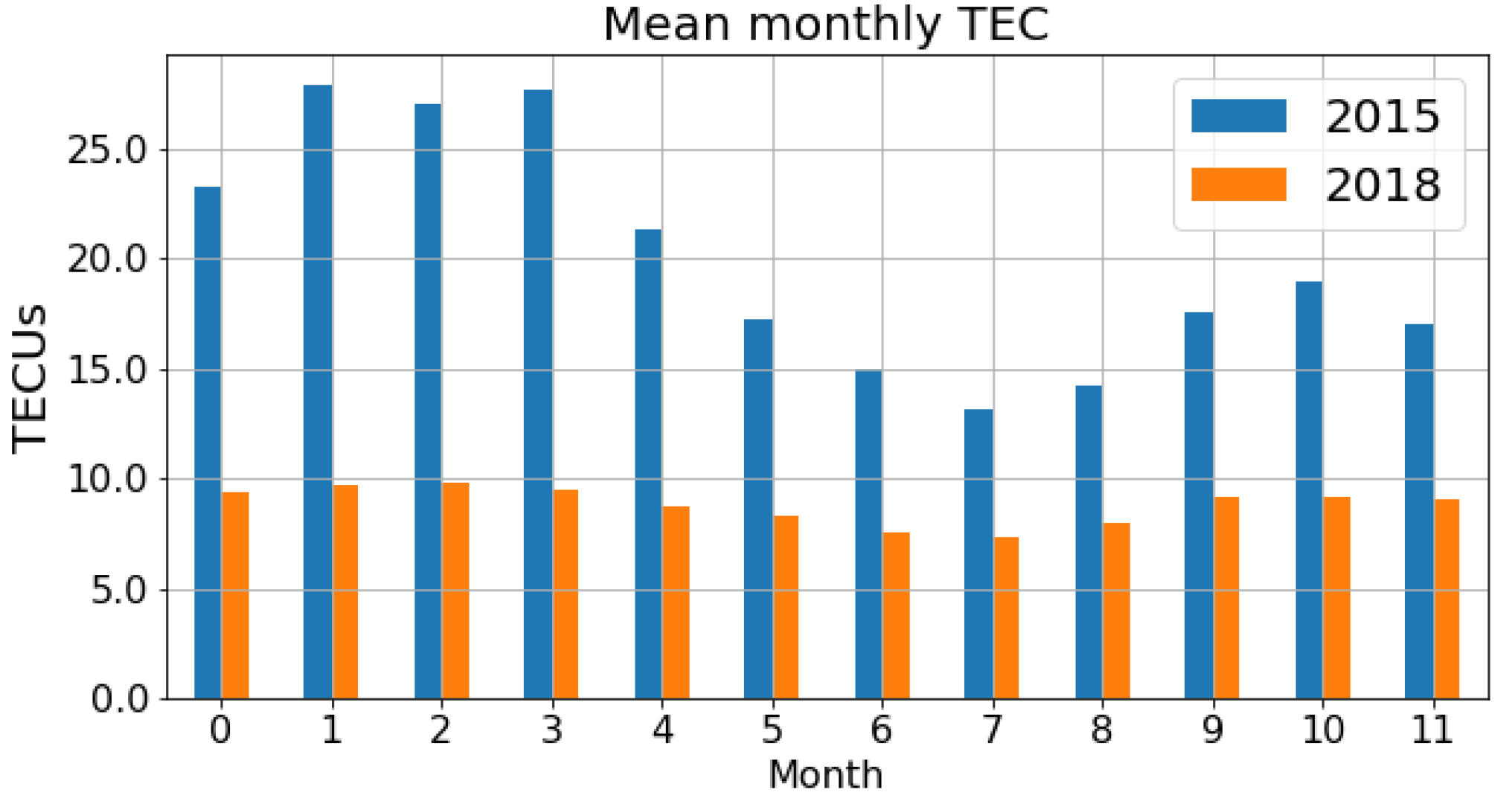
Since the maps have a seasonal component with a mean TEC value that depends on the season of the year (see Figure 1), the search for the nearest map will be carried out in the vicinity of the current month. Therefore, given the date of the current map $Dat{e}_{Test}$, the month is extracted ($M_{Tst}$), and maps the current month and a window of $\pm W_{NeighMonths}$ months are selected from the database. In the experiments, a neighbourhood of $W_{NeighMonths}=1$ was taken. Other parameters are the forecast horizon in hours ($Horizon$) and the number of nearest neighbours ($Nu{m}_{NN}$). The next step is to construct a second database ($D{b}_{Ima}$), which will consist of the maps with the current map month and the neighbouring months for all years. The Euclidean distance between the current map $Map\left(Dat{e}_{Test}\right)$ and the maps in the $D{b}_{Ima}$ database is then calculated (lines 3 to 7 of the Algorithm 1). The vector of distances is then sorted from smallest to largest (line 8 of the Algorithm 1) and assigned to the vector of indices $Inde{x}_{MinDist}$.

We define $Nu{m}_{NN}$ as the number of maps to be used for prediction estimation. The Algorithm 1, lines 9 to 15 describe the process for generating the prediction. For the nearest $Nu{m}_{NN}$ maps, we find the corresponding index $IndexMap$ and the associated date $Date\left[IndexMap\right]$. Next, we add the offset $Horizon$ to generate the date $Dat{e}_{NNMap}$ associated with each of the maps. The maps associated with each date $Dat{e}_{FutMap}\leftarrow Dat{e}_{NNMap}+Horizon$ are combined to generate the future map $Forecas{t}_{Map}$.

Finally, from the maps of the horizon shift, the standard deviation at the pixel level is calculated, as shown in line 17.   

Algorithm 1: The NNGIM algorithm.

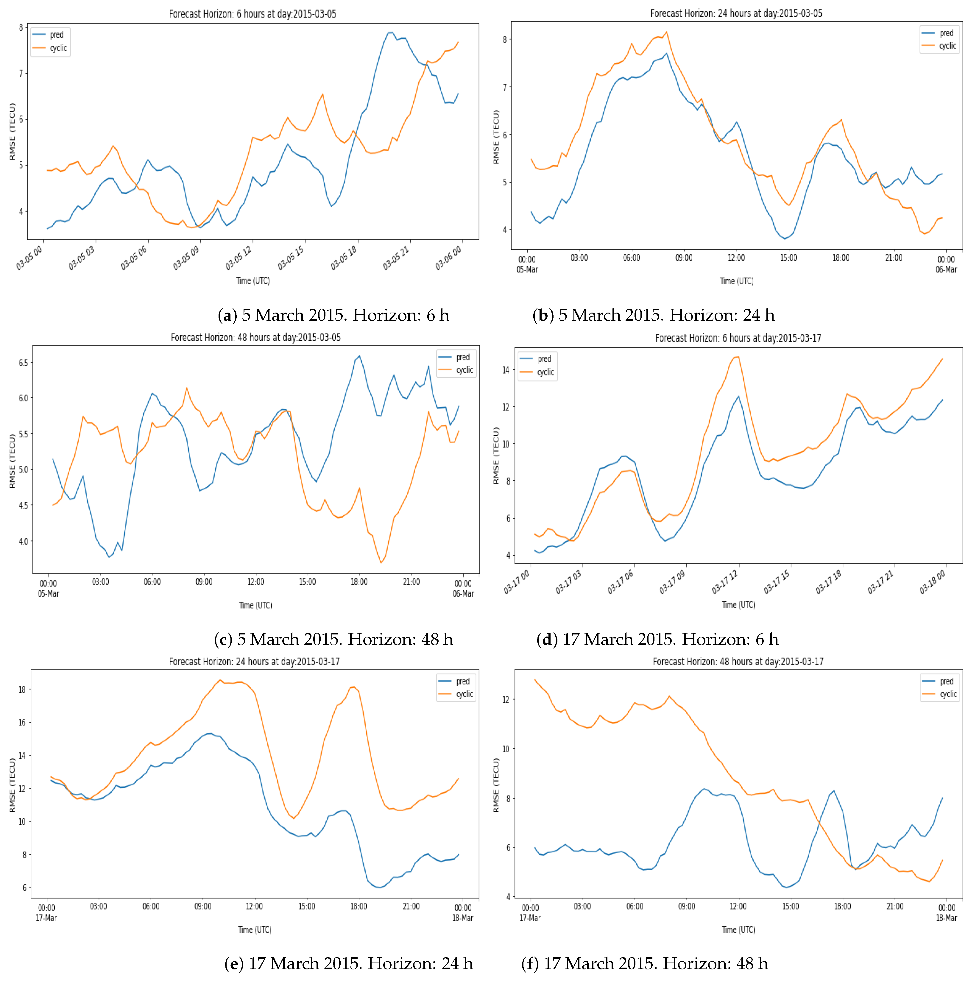
Various strategies for combining the maps were tested, such as a simple average, a distance-weighted average, or weight that diminishes with the time difference. We also tried a trim mean, defined as the average of the values of each specific pixel in the maps, using only the values between the 25th percentile and the 75th percentile. The median of the pixels of the nearest $Nu{m}_{NN}$ maps was also tested. The combination that gave the best results was a simple average of the maps.

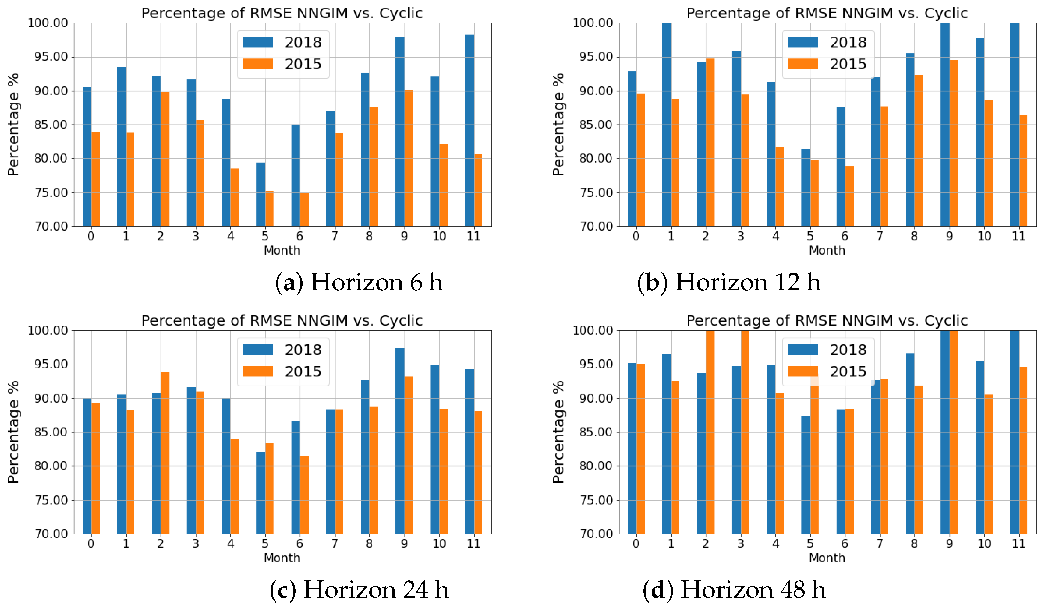
One parameter to be adjusted is the number $Nu{m}_{NN}$ used to calculate the forecast. This value depends on the forecast horizon and the month of the year. For all experiments we chose a value $Nu{m}_{NN}$ = 500. The choice was made based on the performance during June 2019 and was explored for values between 1 and 1000. The rationale for the choice of date was to have a date in a cycle (C24) different from the cycle in which the results are presented (C23), and also at a season of low activity. The experiments showed that for this month and horizons between 3 h and 48 h the optimum value was between 150 and 700. In the real-time implementation, a look-up table will be used in which the month and horizon will be related to the $Nu{m}_{NN}$ value.

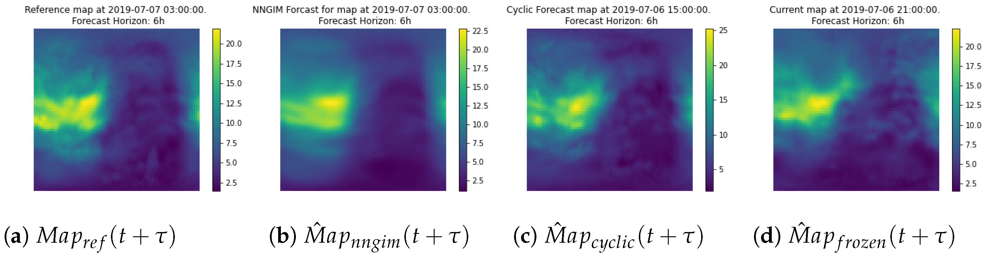
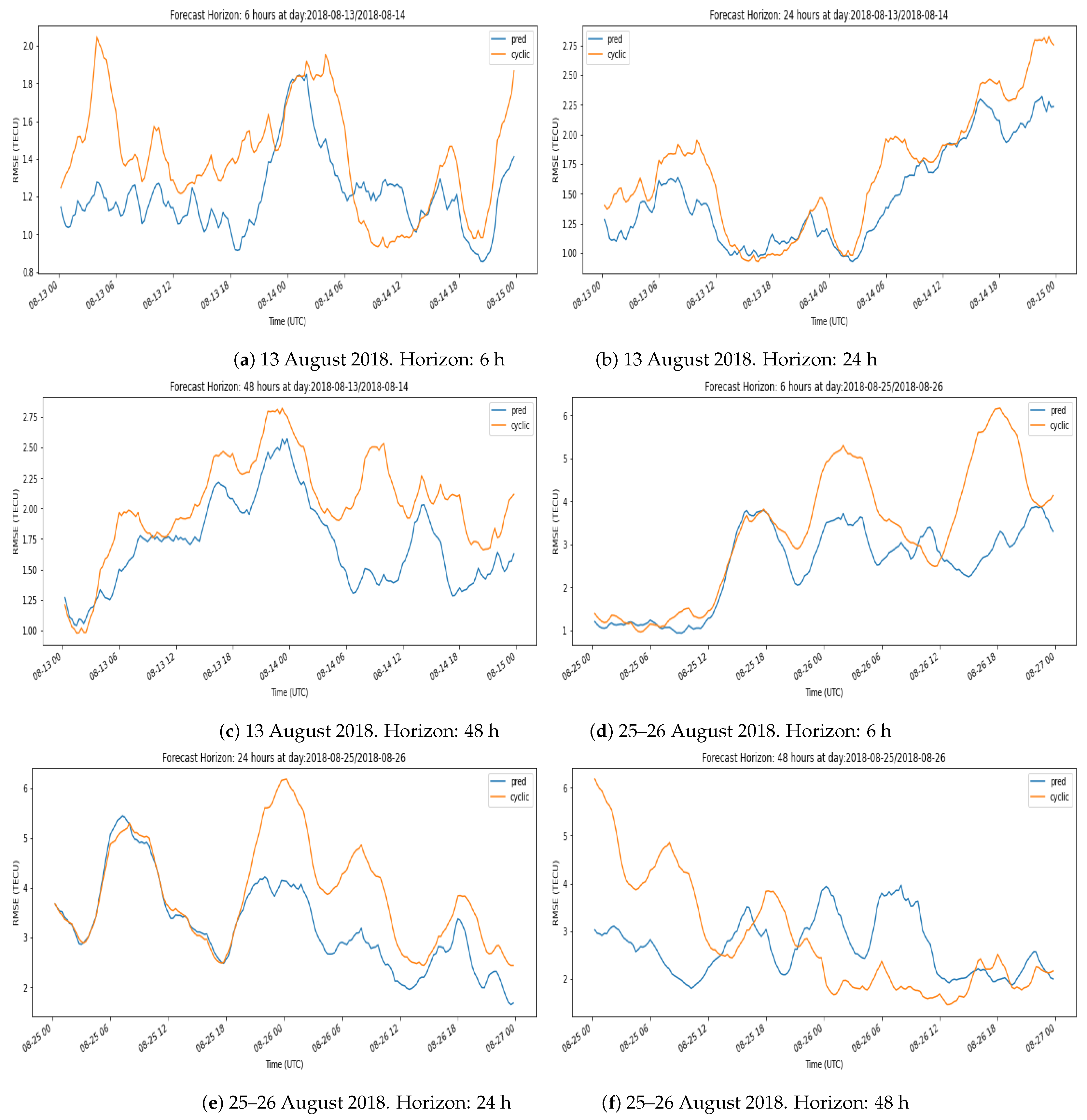
An interesting result is that using only the nearest neighbour, i.e., $Nu{m}_{NN}$ = 1 provided results with a quality equal to using the cyclic version of the map, (defined as $\widehat{M}a{p}_{cyclic}(t+\tau )=Map(t-24h+\tau )$). The performance did not improve until using a number of $Nu{m}_{NN}$ greater than 50. This leads us to think that the use of a large number of maps allows us to create a representation of the possible contributions of the factors that affect ionisation. The explanation is that the combination of external factors is larger than the number of examples in the database. The underlying assumption is that the current combination of factors affecting ionisation can be expressed as a linear combination of similar situations in the past.

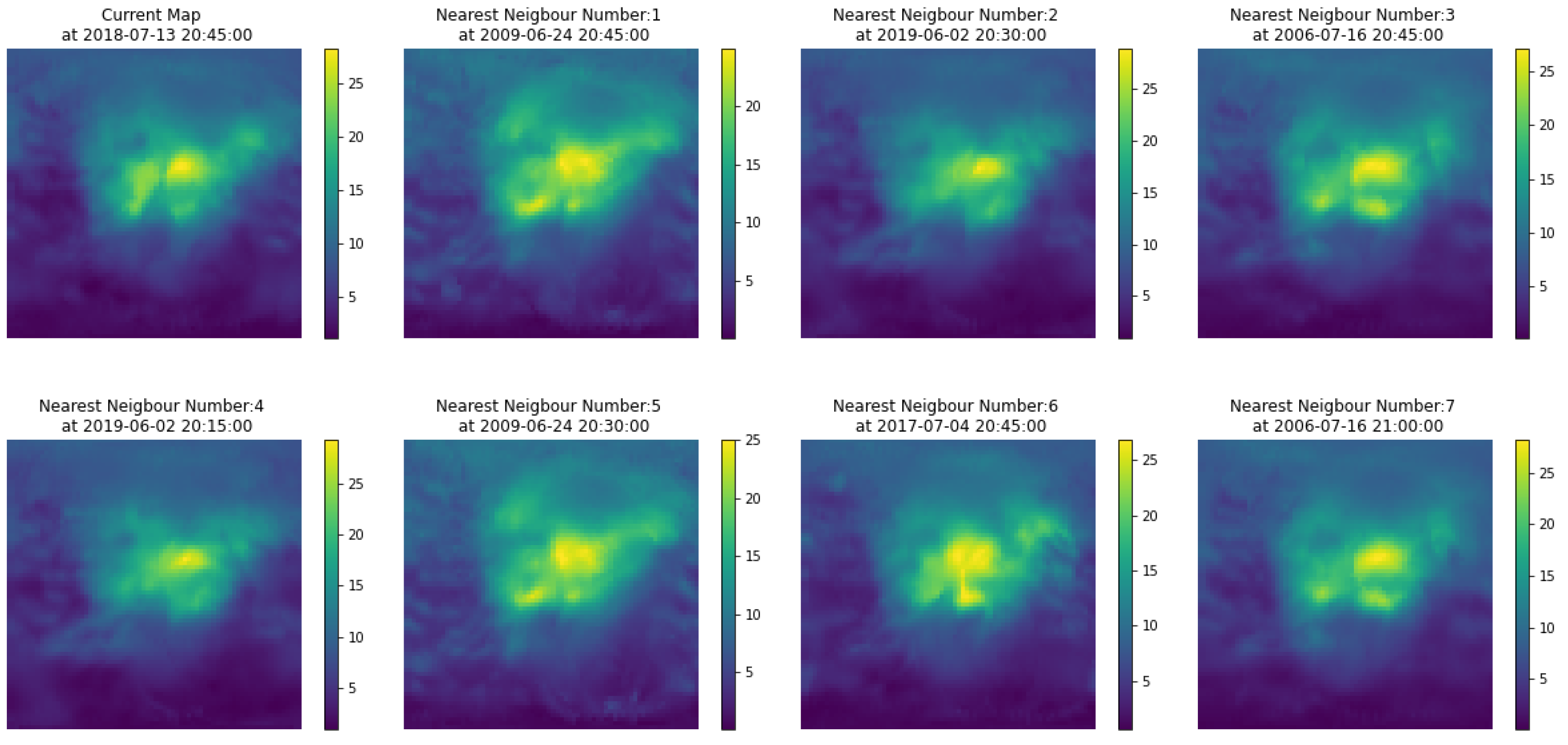
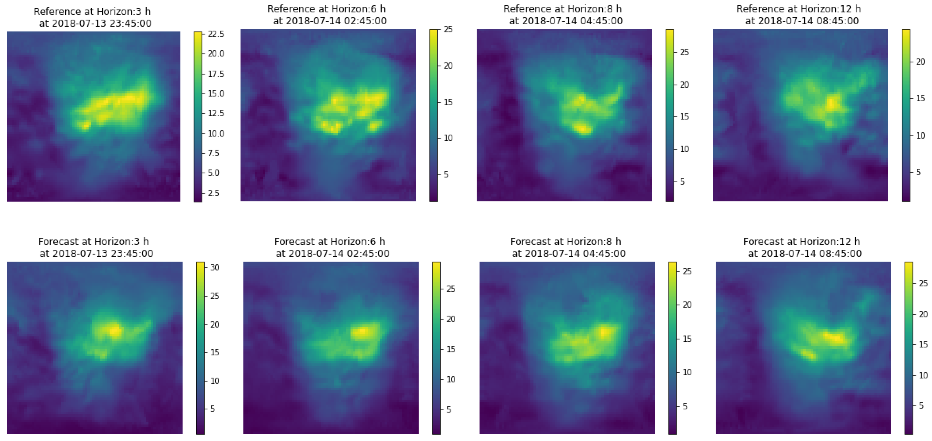
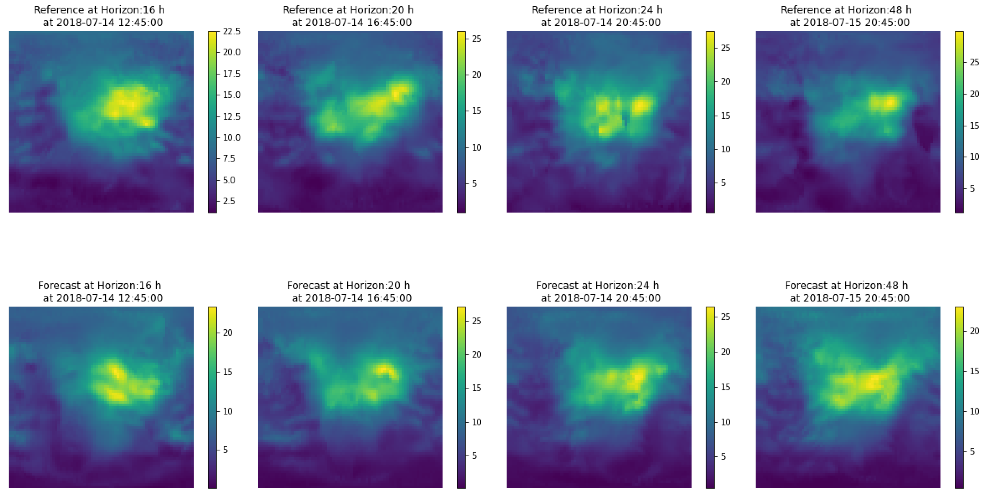
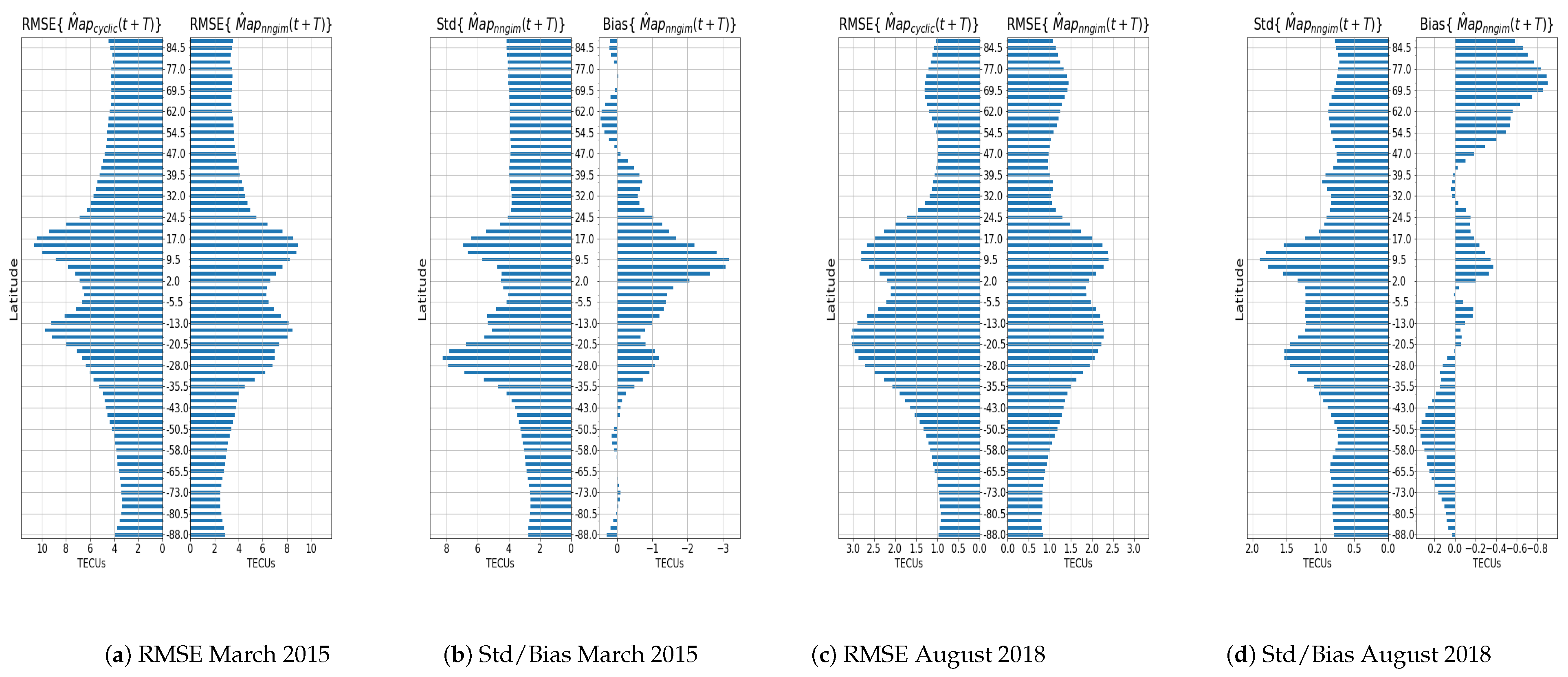
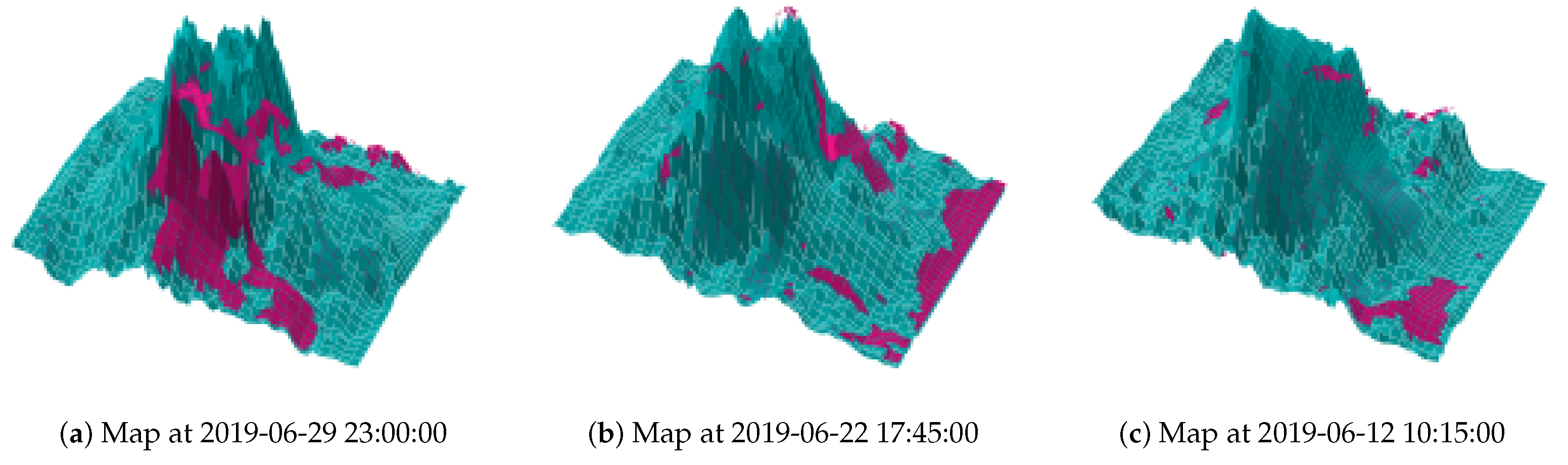
A product of this algorithm is that it can provide confidence intervals for the GIMs, i.e., the local standard deviation of the ionisation values. The estimation of confidence intervals can be done directly, as a collection of several hundred maps is available. One of the features of the maps from which the prediction is constructed is the variability around a central value, as shown in Figure 2. Therefore from the set of maps used to generate the prediction, one can estimate a standard deviation $Forecas{t}_{Map}^{Std}$ at a pixel level, defining this standard deviation as the deviation of the maps from the mean value of the prediction $Forecas{t}_{Map}$. One point that we show in Section 4.1 is that the prediction covers most of the area of the reference map $Re{f}_{Map}$, so we can consider that this variance provides us with an adequate measure of uncertainty for the prediction.

Parameter setting. The algorithm has two parameters to be adjusted, which are the window in months to select maps, denoted as $W_{Neigh}$ and the number of elements to calculate the mean value of the nearest neighbors, denoted as $Nu{m}_{NN}$. The criterion to adjust the parameters was to fit on a subset of the training base (the test was not used at any time for adjustment). In the case of $W_{Neigh}$, which corresponds to the neighboring months, it was observed that due to the variation of the algorithm itself, examples were always selected either from the current month or from the neighboring months. In order to limit the calculation needs, the calculation of distances was limited to the intervals determined by this variable. As for the $Nu{m}_{NN}$ variable, the result is different from the normal application of the Nearest Neighbour (NN) algorithm, in the sense that in order to compensate for the specific variability of each example used for the prediction, the number of neighbors to be used is much higher than in normal applications of the NN. In our case, the prediction error decreased monotonically until reaching a NumNNN value of about 500, producing a plateau of error with small oscillations of the error until reaching about 1500, and at this point the error starts to increase. Note that the fraction of elements used is small with respect to the total number of examples which exceeds one million.

To see the effects of adjusting these parameters, see illustration of how the algorithm works (Section 2.3) and example of forecasts at several horizons (Section 2.4).

Improvements: The improvements we envisage in the next step are to change the average distance, using a metric on the manifold in which the map is located. This is the distance defined in [20] in which coefficients of the angle between coordinates $g_{i,j}=<e_i,e_j>$ are used to weight the Euclidean distance. The advantage of using this distance is that it allows considering in the similarity measure between maps, distortions such as shifts, rotations, etc. The reason why it has not been used in this implementation is that it requires a computational load proportional to the square of the number of map elements. With the current hardware capabilities at 2021, the computation of $Ma{t}_{Dist}$ took about ten minutes, so it was not implemented in the final prototype.

Another improvement is to use a heuristic that decreases the computational needs to determine the nearest neighbors. That is, an algorithm with a suitable heuristic for the dimensionality of the maps and with a lower search cost, as is the case of [21]. The fact that the GIMs have the ionisation levels distributed in clear and distinct regions makes this algorithm efficient. This might allow implementing a distance with higher computational cost as the nearest neighbour search cost can be decreased.

The computational cost on an iMac i7 using one core of applying the algorithm was as follows. The Euclidean distance $Ma{t}_{Dist}$ from a map $Map\left(Dat{e}_{Test}\right)$ to the database $D{b}_{Ima}$ consisting of the current month and the two neighbouring months (with 170,000 maps) was of the order of 135 ms, and the cost of sorting the distances $Argsort\left(Ma{t}_{Dist}\right)$ of 9 ms, the calculation of the average map $Forecas{t}_{Map}$, was less than 1 ms.

The format of the maps consisted of TEC values measured with a resolution of 2.5 degrees in latitude and 5 degrees in longitude, resulting in maps represented as a 72 × 71 array of floats. Each map occupied 40 k bytes on disk (the float represented in ascii format had only one decimal place), while in memory it occupied 164 k bytes with a float-32 bit representation. For more information see Section 2.1

The most time-consuming part of the algorithm is the loading into memory of the pre-computed database $D{b}_{Ima}$, which occupies 2 gigabytes. The time cost on an SSD is in the order of 2 s. However, in a real-time application, the database can be kept permanently in memory.

The real-time prediction of the implementation of this algorithm can be found at the following URL: [22], with the following naming convention:

The three regions where the forecast was done: Global Forecast (un*g), North-Pole Forecast (un*n), South-Pole Forecast (un*s) And the different horizons that were implemented in real time:

1

un0g/un0n/un0s: 1 h Forecast

2

un1g/un1n/un1s: 6 h Forecast

3

un2g/un2n/un2s: 12 h Forecast

4

un3g/un3n/un3s: 18 h Forecast

5

un4g/un4n/un4s: 24 h Forecast

6

un8g/un8n/un8s: 48 h Forecast

The polar predictions consist of segments of the global map clipped at 45 degrees of latitude.

2.3. Illustration of How the Algorithm Works

To understand how the algorithm works, we will consider two points of view.

1.

How the dates of the nearest maps are distributed along the solar cycles: C23, C24 and C25.

2.

Examples of actual maps to understand how is the variability of the nearest neighbours.

We will perform the analysis on day 2019-05-21 16:15:00 UTC a C25 cycle day during summer.

1.

In Figure 3 we show that the nearest neighbours are distributed over years in the same phase of the cycle. Using only examples from the two cycles C23 and C24. The algorithm does not select any maps from the previous month, and most of the closest maps are from the next month. As we will see later, there is a significant dependence of the behaviour of the algorithm on the month in which the prediction is made. As for the time of day, most of the examples are at the same time of day plus or minus one hour.

2.

Next, we consider the variability of the closest maps. The variability of these maps reflects the ionospheric conditions that are common and those that differ. In Figure 2 we show the map for 2018-07-13 20:45:00 UTC and the first seven nearest neighbours in the Euclidean distance sense. In the experiment we used 500 nearest neighbours to estimate the forecast. Examples of prediction are shown in Figure 4, Figure 5 and Figure 6. To help make it easier to compare, we present the maps in sun-fixed geomagnetic coordinates, which are the setting in which the software computes the distance between maps. The selected maps are from the same time of the year and at similar moments of the solar cycle. On the other hand, the morphology is variable, which indicates that each of the maps reflects ionospheric conditions that have parts in common with the current map as well as specific components. The hypothesis underlying the NNGIM model is that the components common to the current map are preserved by the average, and those that are not common are smoothed out. This variability around common values allows to estimate confidence intervals can capture the most likely ranges in the true reference value. The maps at a future shift equal to the prediction horizon exhibit very similar visual features. For reasons of space and similarity between figures, we do not show them.

2.4. Example of Forecasts at Several Horizons

In Figure 4 and Figure 5 we show a selected sequence of predictions for the map at 2018-07-14 20:45:00 UT, at horizons ranging from 3 h to 48 h. In the first row we show the reference to 3 h, 6 h, 8 h, and 12 h horizons, and in the second row we show the prediction result. The third and fourth rows show the results for horizons of 16 h, 20 h, 24, 48 h. In order to assess the results it has to be taken into account that the colour bars are not at the same scale. This means that local maxima can distort the level of the overall colour gradation. In any case, an indication of the effectiveness of the algorithm lies in comparing the medium/high ionisation regions (not maxima) between reference and prediction. In these cases, the shape of the regions is found to be similar.

Note that the figures use as color code the ’viridis’ scale instead of the more usual ’jet’ scale. The reason is that the ’viridis’ color scheme implements a linear scale with brightness going from dark black to bright yellow linearly, while the ’jet’ scale has the brighter colors at the middle of the scale (blue/yellow), and the lowest/highest values are coded with the darker colors. This non monotonicity of the relationship color/brightness creates ambiguities.

2.5. Selection of the Benchmark

In this section, we will define the benchmark to assess the performance of the algorithm. A standard reference to evaluate the predictions are the CODE predictions made by NOAA [23] (see Section 4.2). Another commonly used reference as benchmark predictor is either a prediction using the current frozen map or as a prediction the cyclic map, that is, the immediately preceding map of the same time as the time to be predicted. We will formally define the two predictors as follows:

• Frozen: $\widehat{M}a{p}_{frozen}(t+\tau )=Map\left(t\right)$
• Cyclic: $\widehat{M}a{p}_{cyclic}(t+\tau )=Map(t-24\mathrm{h}+\tau )$

In Section 4.2 we present the comparison with the NOAA forecast product.

As a benchmark in the following sections, we will use the cyclical prediction $\widehat{M}a{p}_{cyclic}(t+\tau )$.

We argue this decision through

Table 4. Forecasting RMSE (TECU) for $\widehat{M}a{p}_{frozen}(t+\tau )$ vs. $\widehat{M}a{p}_{cyclic}(t+\tau )$ (June 2019).

Horizon: $\mathit{\tau }$ (hours)	3 h	6 h	8 h	12 h	16 h	20 h	24 h	28 h	32 h	36 h	48 h
$\widehat{M}a{p}_{frozen}(t+\tau )$ (TECU)	1.87	2.35	2.51	2.59	2.51	2.18	1.42	2.19	2.57	2.61	1.54
$\widehat{M}a{p}_{cyclic}(t+\tau )$ (TECU)	1.43	1.43	1.41	1.45	1.41	1.42	1.42	1.42	1.42	1.44	1.42

, in which we show the prediction errors in RMSE (TECU) for prediction horizons ranging from 3 h to 48 h. In this case, one can see that the prediction cyclic $\widehat{M}a{p}_{cyclic}(t+\tau )$ RMSE error and the standard deviation are constant regardless of the prediction horizon, and equal to the 24-h error of the frozen predictor $\widehat{M}a{p}_{frozen}(t+\tau )$. This is to be expected since at all times the cyclic predictor behaves as a 24-h predictor. On the other hand, an important limitation of the use of the frozen prediction $\widehat{M}a{p}_{frozen}(t+\tau )$ as a benchmark is that the comparison is made under non-comparable ionospheric conditions. This results in a sinusoidal behaviour of the RMSE, which increases from 3 h to 12 h and then decreases to a minimum at 24 h. This behaviour is then repeated, reaching a new minimum at 48 h. Therefore, since the frozen version $\widehat{M}a{p}_{frozen}(t+\tau )$ is a very pessimistic benchmark, and has a component that depends on the time of day, we will use as a benchmark only the $\widehat{M}a{p}_{cyclic}(t+\tau )$.

To get an idea of the differences between benchmarks and NNGIM prediction, in Figure 6 we present the comparison of the reference map (6-h a head ground truth), with the predictions using the NNGIM algorithms, the cyclic and the frozen reference. The cyclic reference provides local features of the TEC distribution similar to the reference map, while the frozen maps have a quite a different geographical distribution of TEC. On the other hand, the NNGIM prediction, despite using maps from other years, captures the structure of the TEC distribution of the reference map.

3. Results

For the analysis of the algorithm, we have selected two years of the C24 cycle and two days of each year. The criterion for selecting the years was to have a sample of one year of high activity in the cycle and one year of low activity. Likewise for the days, in order to contrast the behaviour of the algorithm in the case of storm days vs. quiet days, we chose two storm days of each year and two adjacent days without a storm.

3.1. Analysis of Selected Years: 2015 and 2018

Figure 1 shows the time series of the average monthly TEC value for the two selected years. The first difference observed in the two years is the underlying monthly average TEC level and the fact that in the most active year (2015), the monthly profile of the TEC level has a marked cyclical component with a minimum in the summer. On the other hand, in the least active year (2018), the cyclical component has a lower amplitude. The mean annual TEC value for 2015 is 20 TECU, while in 2018 it is 8.8 TECU.

First, we show the performance of the NNGIM algorithm in TECU values and then for comparison purposes in percentages concerning the prediction using the frozen cyclic.

In

Table 5. RMSE error of the NNGIM algorithm for several horizons.

Horizon	6 h	12 h	24 h	48 h	Mean TECU
2015 (TECU)	3.50	3.70	3.72	4.00	20.0 TECU
2018 (TECU)	1.59	1.66	1.59	1.66	8.8 TECU

we show the average TECU prediction RMSE for 4 prediction horizons. In 2015 the prediction error increases as we increase the horizon from 17% to 20% of the average TEC value. On the other hand, the error in 2018 remains almost constant regardless of the horizon and stands at 18% of the average TEC value in that year. However, as we will see below, the prediction error has an annual cyclical component, being lower in the summer.

In Figure 7 we present the percentage change of the RMSE value for the cyclical prediction vs. NNGIM for various horizons. That is, we plot the ratio

$$\frac{\widehat{M}a{p}_{nngim}(t+\tau )}{\widehat{M}a{p}_{cyclic}(t+\tau )}\times 100\%$$

The first conclusion derived from the figures is that the use of NNGIM provides a decrease that follows an annual pattern and in the summer months for 6 and 12-h horizons provides a decrease in error in the order of 20% to 25%. This contrasts with the experience with tangent spaces predictions (see [3]) and deep learning based methods (see Section 1.2), where a significant degradation in quality is reported at prediction horizons of the order of 6 h. The prediction at 24 and 48 h reported as a percentage of frozen in [9] using deep learning is similar to the one shown in the lower row of Figure 7.

The 12-h forecast results are worse than the 24-h ones except for the months of May and June. This is because this is the moment in the interval $(t,t+24\mathrm{h})$ when the ionosphere configuration is maximally different from the current state.

On the other hand, 48 h seems to be a natural limit for the method, as the error reduction for frozen cyclic is on an annual average of 95%.

3.2. Performance on Selected Days of 2015 and 2018

To evaluate the performance of the NNGIM method, we selected two days at the maximum of cycle 24 and two days at the minimum of the same cycle. The criterion for selecting the days was that one of them coincided with a geomagnetic storm and the other one coincided with a nearby day without significant activity. The selected days were:

1.

17 March 2015 (St.Patrick Day storm) and 5 March 2015 (non storm day).

2.

25–26 August 2018 (storm day) and 13–14 August 2018 (non storm day).

In both cases, the time distribution of geomagnetic activity index (i.e., Kp ) are shown in Table 1, Table 2,

Table 6. Hourly Kp for the 5 March 2015.

Hour	00–03 h	03–06 h	06–09 h	09–12 h	12–15 h	15–18 h	18–21 h	21–00 h
Kp	1	0	0	1	2	2	2	1

and

Table 7. Hourly Kp and 13,14 August 2018.

Hour	00–03 h	03–06 h	06–09 h	09–12 h	12–15 h	15–18 h	18–21 h	21–00 h
Kp (13 August)	1	1	1	1	1	1	0	1
Kp (14 August)	2	1	1	1	1	0	0	2

. The data was obtained from [24].

3.2.1. Performance on 5 and 17 March 2015

In Figure 8 we present the comparison of the NNGIM predictor versus the cyclic frozen for various horizons in the form of a time series, at a rate of one map every 15 min.

In the top row, the performances of NNGIM vs. frozen cyclic are compared for the 5th of March 2015, which is a day with no significant events (see the Table 1 and Table 6). The difference in performance is irregular for the 6-h forecast, while for the 24-h forecast the average reduction over the day is a little more than a 10% error. The worse behaviour towards the end of the day could be due to the increase of the Kp indicator and the presence of three solar flares in close temporal proximity. Since the NNGIM method assumes that similar situations have been seen in the past and are used for prediction, the changes in this particular configuration might not have been seen in the past.

In the bottom row, we show the performance throughout the 17 March 2015 ( Saint Patrick’s Day storm). The RMSE level compared to the 5 March is between two and three times higher. However, in this case, the NNGIM predictor shows on average a better performance than the cyclic frozen with variations depending on the forecast horizon. For the first hours of the day, the NNGIM predictor performs similarly to cyclic frozen, for the 6 and 24-h horizons, improving throughout the day. An interesting behaviour is that at 48 h the RMSE of the NNGIM forecast remains at low levels throughout the day, while the frozen cyclic in the early hours provides twice the error.

3.2.2. Performance on 13–14 and 25–26 August 2018

Figure 9, shows the RMSE time series for the two selected days at a time of the low activity solar cycle. On that day, the RMSE level is similar to that of the 5th of March 2015 analysed above, which was a day of low geomagnetic activity, while being in a high activity phase of the solar cycle.

On 13–14 August 2018, the NNGIM prediction is better or equal to that of the cyclic frozen, except for a brief interval on the 14th of March at a 6-h horizon. The average improvement over the day is in the order of 25% for 6 h, 13% for 24 h, and 18% for 48 h. However, there are significant fluctuations throughout the day and the slopes/error patterns vary from horizon to horizon.

On 25–26 August 2018 (storm day) for the 6- and 24-h horizons NNGIM systematically performs better than the frozen cyclical. The performances at the 6- and 24-h horizons are practically the same for the 25th day, while they differ significantly for the 26th day, with NNGIM being 25–50% better over long time intervals.

3.3. RMSE, Bias and Standard Deviation by Latitude

In this section, we will study the relationship of RMSE with standard deviation and bias. In Figure 10, we show the performance for a horizon $T=6$ h. In the Figure we present by latitude (a) the RMSE of the NNGIM and frozen cyclic predictions and (b) the standard deviation and bias components of the NNGIM. The study period consists of the dates studied above, i.e., August 2015 and May 2018. The values were calculated on 3007 maps corresponding to 31 days, with maps every 15 min.

The first observation is that the NNGIM prediction has a lower RMSE at all latitudes on the two studied dates. The RMSE maxima are located in the case of NNGIM at the same latitude, while in the case of frozen cyclic the latitude in one case differs. On the other hand, the maxima in the standard deviation do not coincide with the RMSE maxima, noting that the difference is explained in the case of March 2015 by a very high bias at about 10 degrees north latitude. The bias of -3 TECU observed in this case is rare, in the maps observed by the author, the bias, in general, was less than 1 TECU, as illustrated in the case of August 2018.

4. Discussion

4.1. Reliability and Confidence Margins of the NNGIM Algorithm

In this section, we will study the reliability of the standard deviation estimated from the nearest neighbours provided by the algorithm. The purpose is to show that the standard deviation computed on the nearest future maps correctly represents the variability of the predicted map. We will show the reliability from two points of view, the first one consists of plotting several maps and showing the regions not covered by the confidence margin (defined as one standard deviation around the mean TEC value at each geographic coordinate of the GIM map, i.e., we associate a margin of about 68% confidence with each interval of 2.5 degrees latitude by 5 degrees longitude) given by the standard deviation provided by NNGIM. The second point of view will consist of showing the decrease in the error obtained when the prediction is considered to be included within the confidence margin given by the standard deviation.

In Figure 11, we show maps for different dates for the month of June 2019, in which we mark in green the region covered by the interval $Forecas{t}_{Map}\pm Forecas{t}_{Map}^{Std}$, and in red the areas of the prediction that fall outside this interval. The images show that the areas of the $Forecas{t}_{ref}$ maps not covered by a standard deviation margin are located in the periphery or at the areas of sharp transition.

In Figure 12 we show the error decrease regarding the NNGIM prediction if we consider only data outside the interval within the confidence margin. That is, we consider the error to be zero if the predicted map is contained in the margin, i.e., $Forecas{t}_{ref}\subset Forecas{t}_{Map}\pm Forecas{t}_{Map}^{Std}$. It is seen that systematically for the two years and prediction horizons, the error decreases between 15 and 20%. In other words, assuming the correct value is within the confidence interval significantly reduces the error. An interesting feature is that this error reduction does not depend on either the season of the year or the prediction horizon.

4.2. Validation of the Method with JASON3 and CODE Data

Next we show the results of the validation of the NNGIM VTEC in terms of the differences with respect to JASON3 VTEC measurements (see Figure 13) and the comparison with other GNSS VTEC products in terms of Bias, Variance and RMS (see Figure 14).

This part of the study was conducted in the interval of the first 100 days of the year 2021. Note that for the sake of completeness of the analysis of the method, we have performed the experiments at different times of the solar cycle. Given the space limitation, we think that in this way we can provide the maximum information of the algorithm from the point of view of each issue to be evaluated. The CODE data was downloaded from the NOAA website [23].

The comparison was made between the products based on NNGIM prediction at 24 h (UN4G) and 48 h (UN8G), vs. IGSG and Center for Orbit Determination in Europe (CODE) VTEC prediction model products, at 24 h (C1PG) and 48 h (C2PG).

In Figure 13, we show the histogram of the VTEC residual defined as $\delta V=VTE{C}_{JASON3}$$-VTE{C}_{ForecastGIM}$ on a logarithmic scale to enhance the details in the low-density parts of the histogram, i.e., regions where the number of samples per bin is much lower than at the mode of the distribution. For comparison purposes on the figure, there is a summary of the relevant statistics of each product, i.e., bias, standard deviation, and RMS. Note that the Std. Dev and RMS of the NNGIM prediction at 24 h (UN4G) and 48 h (UN8G) are systematically lower than the CODE and IGSG. Note that the tails of the distributions are similar. Furthermore, the distribution related to the NNGIM product having a lower width compared with the CODE products. This indicates that the probability of a high-value positive error in the NNGIM products is much lower than the other products.

Next, we will compare, concerning the JASON3 measurements, the products by latitude, as a function of the differences in standard deviation, bias, and RMS.

In Figure 14, on the left, we show the standard deviation of the VTEC residual vs. JASON3 at 5-degrees longitudinal intervals. Note that the standard deviation is weighted by the number of JASON3 observations in cells in the same 5-degree latitude range. The 24-h prediction product based on NNGIM, UN4G consistently has a lower standard deviation than the equivalent CODE, C1PG except for the sample at 15 degrees latitude north where they are the same. The largest differences are observed at the equator and in areas of north/south latitude greater than 35 degrees. In the case of the 48-h forecast products (UN8G vs. C2PG), the trend is very similar, with NNGIM having a lower standard deviation at all latitudes except at 15 degrees north latitude.

In Figure 14, in the center, we show the bias of the products. In this case, the bias of the NNGIM products is lower, except in the region below −35 degrees south latitude and above 45 degrees north latitude. The explanation for this bias corresponds to the fact that there is a different ionosphere sampling model, as explained in [19].

Finally, in Figure 14, on the right, we show the RMS value by latitude, in this case, the RMS of the prediction is better for the NNGIM products between −30 degrees south latitude and 50 degrees north latitude. Note that from 50 degrees north latitude the difference concerning CODE is less than half a TECU, and on the other hand in the equatorial region the UN4G and UN8G products provide an improvement of 2 TECUs. The difference in the south polar region could be because there are fewer stations, and therefore the GIMs are less accurate.

Note that the availability of the NNGIM forecasting depends on the delay of generating the GIM maps, which is the case of the UPC-IonSAT is of about half an hour, while the availability of the CODE maps can be with a delay of up to 5 or 7 h, which makes the effective forecasting horizon shorter.

4.3. Considerations about the Quality Assessment by Means of JASON3 VTEC Measurements

The importance of the VTEC measures obtained by JASON3 lies in the fact that it provides us with an objective reference of the real value for the comparison purposes. The measures provided by JASON3 allow us to determine whether the estimate made by the prediction product provides a correct value or introduces biases. As the orbit altitude of JASON3 is about ∼1300 km, the altimeter can count almost all the VTEC of the ionospheric state above the ocean region. It is important to emphasize that over the ocean areas, the GIM used for the prediction might have large interpolating errors appearing due to their far distance from GNSS ground stations. Therefore, the use of JASON3 VTEC measurement allows for a critical evaluation of the forecast products in adverse circumstances. In this work, the raw observations of the JASON3 VTEC were preprocessed to reduce the measurement noise. The process carried out included the use of a temporal sliding window, removal of outliers, and so on, as explained in [25,26].

Evaluation using dSTEC may be an alternative for evaluating VTEC values of GIM prediction products. However, in this particular case the use of dSTEC may not be appropriate because of the following. Typically, the JASON3 VTEC assessment is a validation method for GIMs only over the ocean region, so it may be appropriate to consider the complementary assessment for GIMs over the land region, namely the dSTEC assessment, which compares the difference between the observed STEC along the phase-continuous satellite-station arc and the calculated STEC from GIM, see details in [25]. However, the usage of altimeter VTEC measurements to assess GIMs has been proven to be a good external assessment procedure, consistent with other methods based on GNSS data (behaving similarly to the dSTEC test [25]) but independent from GNSS and globally distributed. These are the main reasons behind focusing on altimeter data, being the JASON3 the one available during the whole period of analysis, see the former studies that used JASON2, JASON1, and TOPEX altimeters.

4.4. Explanation of the Limitation of Saturating Nonlinearities

The learning algorithms used in LSTM type neural networks employ the gradient associated with internal nonlinearities of hyperbolic tangent or sigmoid type. Both nonlinearities, as illustrated (hyperbolic tangent case) in Figure 15 (right), saturate for large absolute values, and the derivative is zero. The consequence of this is that the gradient used for estimating the weights of the neural networks in the high value regions is practically zero, and therefore no learning takes place. In long tail distributions (e.g., Kp, Solar Flux, Magnetic Field Index proton density, EUV radiation, etc.), with a morphology as shown in Figure 15 left, and histograms with outliers. It is the case that the learning algorithms have precisely the null gradient in cases of greatest interest from the point of view of prediction. Therefore, the estimation of the neural network weights becomes zero in the cases of extreme activity.

5. Conclusions

In this work, we have introduced a method to predict GIMs at various horizons based on the Nearest Neighbour technique. This technique allows predictors to be implemented without the need to train a model, and the computation time is small. The assumption on which the model is based is that a database covering more than one solar cycle is available, and that the geomagnetic conditions affecting the current map have somehow happened in the past, and that similar geomagnetic effects are distributed among several maps, whose linear combination allows a better approximation of the prediction. An advantage of the method is also that from the similar maps found in the historical database, a confidence margin can be created. The prediction using this confidence margin allows a significant decrease in the prediction error. We have performed a real-time implementation. The computational cost of adding a prediction horizon is very low, so in the implementation, predictions are made with almost no additional cost for arbitrary horizons. The prediction results improve compared to the frozen cyclic up to a 48-h horizon, which seems to be a natural barrier for this method. Finally, the method has been assessed in different moments of the solar cycle, taking into account days with storm and without significant geomagnetic perturbations. Additionally, the method has been assessed by comparing with the forecast at 24 and 48 h of the Center for Orbit Determination in Europe (CODE) prediction model products.

References

1. García-Rigo, A.; Monte, E.; Hernández-Pajares, M.; Juan, J.M.; Sanz, J.; Aragón-Angel, A.; Salazar, D. Global prediction of the vertical total electron content of the ionosphere based on GPS data. Radio Sci. 2011, 46, 1–3. [Google Scholar] [CrossRef] [Green Version]
2. Web Page of IonSAT: IonSAT—Ionospheric Determination and Navigation Based on Satellite and Terrestrial Systems. Available online: https://futur.upc.edu/IonSAT?locale=en (accessed on 2 June 2021).
3. Monte Moreno, E.; García Rigo, A.; Hernández-Pajares, M.; Yang, H. TEC forecasting based on manifold trajectories. Remote Sens. 2018, 10, 988. [Google Scholar] [CrossRef] [Green Version]
4. Wang, C.; Xin, S.; Liu, X.; Shi, C.; Fan, L. Prediction of global ionospheric VTEC maps using an adaptive autoregressive model. Earth Planets Space 2018, 70, 1–14. [Google Scholar] [CrossRef] [Green Version]
5. Ian, G.; Bengio, Y.; Courville, A. Deep Learning; MIT Press: Cambridge, MA, USA, 2016. [Google Scholar]
6. Xiong, P.; Zhai, D.; Long, C.; Zhou, H.; Zhang, X.; Shen, X. Long Short-Term Memory Neural Network for Ionospheric Total Electron Content Forecasting Over China. Space Weather 2021, 19, e2020SW002706. [Google Scholar] [CrossRef]
7. Mustafa, U. Deep learning for ionospheric TEC forecasting at mid-latitude stations in Turkey. Acta Geophys. 2021, 60, 589–606. [Google Scholar]
8. Wen, Z.; Li, S.; Li, L.; Wu, B.; Fu, J. Ionospheric TEC prediction using Long Short-Term Memory deep learning network. Astrophys. Space Sci. 2021, 366, 3. [Google Scholar] [CrossRef]
9. Cherrier, N.; Castaings, T.; Boulch, A. Forecasting ionospheric Total Electron Content maps with deep neural networks. In Proceedings Conference Big Data Space (BIDS); ESA Workshop: Toulouse, France, 2017. [Google Scholar]
10. Liu, L.; Zou, S.; Yao, Y.; Wang, Z. Forecasting global ionospheric TEC using deep learning approach. Space Weather 2020, 18, e2020SW002501. [Google Scholar] [CrossRef]
11. Ji, E.Y.; Moon, Y.J.; Park, E. Improvement of IRI global TEC maps by deep learning based on conditional Generative Adversarial Networks. Space Weather 2020, 8, e2019SW002411. [Google Scholar] [CrossRef]
12. Krankowski, A.; Kosek, W.; Baran, L.W.; Popinski, W. Wavelet analysis and forecasting of VTEC obtained with GPS observations over European latitudes. J. Atmos. Sol.-Terr. Phys. 2005, 67, 1147–1156. [Google Scholar] [CrossRef]
13. Weber, G.; Dettmering, D.; Gebhard, H. Networked transport of rtcm via internet protocol (ntrip). In A Window on the Future of Geodesy; Springer: Berlin/Heidelberg, Germany, 2005; pp. 60–64. [Google Scholar]
14. Hernández-Pajares, M. Inputs received from Ionospheric research groups on activities related with RT global electron content determination. In Proceedings of the IGS RT WG Splinter Meeting, Pasadena, CA, USA, 23 June 2014; pp. 1–15. [Google Scholar]
15. Hernández-Pajares, M.; Juan, J.; Sanz, J. New approaches in global ionospheric determination using ground GPS data. J. Atmos. Sol. Terr. Phys. 1999, 61, 1237–1247. [Google Scholar] [CrossRef]
16. Orús, R.; Hernández-Pajares, M.; Juan, J.; Sanz, J. Improvement of global ionospheric VTEC maps by using kriging interpolation technique. J. Atmos. Sol. Terr. Phys. 2005, 67, 1598–1609. [Google Scholar] [CrossRef]
17. Roma Dollase, D.; López Cama, J.M.; Hernández Pajares, M.; García Rigo, A. Real-time Global Ionospheric modelling from GNSS data with RT-TOMION model. In Proceedings of the 5th International Colloquium Scientific and Fundamental Aspects of the Galileo Programme, Braunschweig, Germany, 27–29 October 2015. [Google Scholar]
18. Hernández-Pajares, M.; Juan, J.; Sanz, J.; Colombo, O.L. Application of ionospheric tomography to real-time GPS carrier-phase ambiguities resolution, at scales of 400–1000 km and with high geomagnetic activity. Geophys. Res. Lett. 2000, 27, 2009–2012. [Google Scholar] [CrossRef] [Green Version]
19. Yang, H.; Monte-Moreno, E.; Hernández-Pajares, M.; Roma-Dollase, D. Real-time interpolation of global ionospheric maps by means of sparse representation. J. Geod. 2021, 95, 1–20. [Google Scholar]
20. Wang, L.; Zhang, Y.; Feng, J. On the Euclidean distance of images. IEEE Trans. Pattern Anal. Mach. Intell. 2005, 27, 1334–1339. [Google Scholar] [CrossRef] [PubMed]
21. Omohundro, S.M. Five Balltree Construction Algorithms; International Computer Science Institute Technical Report; International Computer Science Institute: Berkeley, CA, USA, 1989. [Google Scholar]
22. NNGIM Forecasts at Different Horizons. Available online: http://chapman.upc.es/.trial_urtg/tomion/forecast_nngim/quick/last_results/ (accessed on 2 June 2021).
23. Code Data. Available online: ftp://ftp.nodc.noaa.gov/pub/data.nodc/ (accessed on 2 June 2021).
24. Space Weather Live. Available online: https://www.spaceweatherlive.com/ (accessed on 2 June 2021).
25. Hernández-Pajares, M.; Roma-Dollase, D.; Krankowski, A.; García-Rigo, A.; Orús-Pérez, R. Methodology and consistency of slant and vertical assessments for ionospheric electron content models. J. Geod. 2017, 91, 1405–1414. [Google Scholar] [CrossRef]
26. Roma-Dollase, D.; Hernández-Pajares, M.; Krankowski, A.; Kotulak, K.; Ghoddousi-Fard, R.; Yuan, Y.; Li, Z.; Zhang, H.; Shi, C.; Wang, C.; et al. Consistency of seven different GNSS global ionospheric mapping techniques during one solar cycle. J. Geod. 2018, 92, 691–706. [Google Scholar] [CrossRef] [Green Version]
Figure 1. Mean monthly TEC for the years 2015 (in blue) and 2018 (in orange).
Remotesensing 14 01361 g001
Figure 2. Current map at 2018-07-13 20:45:00 UTC (subplot at upper left corner), and the seven Nearest Neighbours. All maps in sun-fixed geomagnetic coordinates. The maps range in latitude from 90 degrees north to 90 degrees south, and in longitude from 180 degrees west to 180 degrees east. Color bars are in TEC units.
Remotesensing 14 01361 g002
Figure 3. Nearest maps are distributed along solar cycles C24 and C25. Histograms of the years (left), months (center) and time of day (right) of the nearest maps to the map at 2019-05-21 16:15:00 UTC.
Remotesensing 14 01361 g003
Figure 4. Selected sequence of predictions for the map at 2018-07-14 20:45:00 UT. The upper row shows the reference to 3 h, 6 h, 8 h, and 12 h horizons, the second row shows the prediction result. Note that the color bars are not at the same scale. The maps range in latitude from 90 degrees north to 90 degrees south, and in longitude from 180 degrees west to 180 degrees east. Color bars are in TEC units.
Remotesensing 14 01361 g004
Figure 5. Selected sequence of predictions for the map at 2018-07-14 20:45:00 UT. The upper row shows the reference to 16 h, 20 h, 24, 48 h, the second row shows the prediction result. Note that the color bars are not at the same scale. The maps range in latitude from 90 degrees north to 90 degrees south, and in longitude from 180 degrees west to 180 degrees east. Color bars are in TEC units.
Remotesensing 14 01361 g005
Figure 6. Comparison of the reference map (a) at 2019-07-07 03:00:00 UTC, with the NNGIM prediction, (b), with the cyclic prediction, (c) and with the frozen prediction (i.e., using current map) (d) with the frozen map. Note that the maps are in the original coordinates, not in the sun-fixed geomagnetic coordinates.
Remotesensing 14 01361 g006
Figure 7. Percentage of RMSE reduction with regard to cyclic freezing for the horizons of 6 h, 12 h, 24 h, 48 h.
Remotesensing 14 01361 g007
Figure 8. Comparison of the NNGIM forecast vs. frozen cyclic RMSE. Upper row: 5 March 2015 (12 days before the storm). Lower row: 17 March 2015 (the St.Patrick storm day).
Remotesensing 14 01361 g008
Figure 9. Comparison of the NNGIM forecast vs. frozen cyclic RMSE. Upper row: 13–14 August 2018 (12 days before the storm). Lower row: 25–26 August 2018 (storm day).
Remotesensing 14 01361 g009
Figure 10. Performance for a horizon T = 6 h. RMSE, bias and standard deviation by latitude. (a) Comparison of the RMSE between the NNGIM and the frozen cyclic March 2015, (b) standard deviation and bias for the NNGIM March 2015, (a) Comparison of the RMSE between the NNGIM and the frozen cyclic August 2018, (b) standard deviation and bias for the NNGIM August 2018. Note that the bias and standard deviation are not the same scale.
Remotesensing 14 01361 g010
Figure 11. Forecast maps in which the basemap coincides with the global coordinates (latitude ± 90 degrees, longitude ± 180 ), and the height shows measured TEC values. The colors distinguish, (green), the regions of the GIM map where the prediction is within the ± sigma range, and in red the regions where the prediction is outside. Green areas: show the areas where the reference F o r e c a s t r e f is included in F o r e c a s t M a p ± F o r e c a s t M a p S t d . Red areas: areas where F o r e c a s t r e f is outside the margin.
Remotesensing 14 01361 g011
Figure 12. Performance for F o r e c a s t r e f F o r e c a s t M a p ± F o r e c a s t M a p S t d . Percentage of RMSE reduction with regard to cyclic freezing for the horizons of 6 h, 12 h, 24 h, 48 h.
Remotesensing 14 01361 g012
Figure 13. Histogram, in log scale for the number of counts, of VTEC difference of JASON3 measurement minus GIMs value for the first 100 days of 2021, the color code indicates the comparison for different forecasting products. The histogram of the reference values of JASON3 is represented in gray. The corresponding overall bias, standard deviation (Std.Dev.), and RMS are indicated in the upper right legend.
Remotesensing 14 01361 g013
Figure 14. Jason assessment for latitudinal zones, the color representing different products. Note that the measures are weighted by the number of JASON3 observations in cells with the same 5-degree intervals of latitude. Blue: UN4F, Orange: UN8G, Green: C1PG, Red: C2PG, Purple: IGSC.
Remotesensing 14 01361 g014
Figure 15. (Left) Example of a time series with a Long Tail distribution, (Center) Histogram of the time series, (Right) Comparison of the Tanh nonlinearity with its’ derivative.
Remotesensing 14 01361 g015