
Spatiotemporal Patterns and Driving Force of Urbanization and Its Impact on Urban Ecology
by
 ,
,
Meng Zhang
1,2, 
Huaqiang Du
2,3,4 ,
,
Guomo Zhou
1,2,3,4,*,
Fangjie Mao
2,3,4,
Xuejian Li
2,3,4,
Lv Zhou
1,2,
Di’en Zhu
1,2,
Yanxin Xu
2,3,4 and
Zihao Huang
2,3,4 1
The College of Forestry, Beijing Forestry University, Beijing 100083, China
2
State Key Laboratory of Subtropical Silviculture, Zhejiang A & F University, Hangzhou 311300, China
3
Key Laboratory of Carbon Cycling in Forest Ecosystems and Carbon Sequestration of Zhejiang Province, Zhejiang A & F University, Hangzhou 311300, China
4
School of Environmental and Resources Science, Zhejiang A & F University, Hangzhou 311300, China
*
Author to whom correspondence should be addressed.
Remote Sens. 2022, 14(5), 1160; https://doi.org/10.3390/rs14051160
Submission received: 25 December 2021
/
Revised: 9 February 2022
/
Accepted: 23 February 2022
/
Published: 26 February 2022
(This article belongs to the Special Issue Urban Planning Supported by Remote Sensing Technology)
Abstract
:Urbanization inevitably poses a threat to urban ecology by altering its external structure and internal attributes. Nighttime light (NTL) has become increasingly extensive and practical, offering a special perspective on the world in revealing urbanization. In this study, we applied the Normalized Impervious Surface Index (NISI) constructed by NTL and MODIS NDVI to examine the urbanization process in the Yangtze River Delta (YRD). Geographical detectors combined with factors involving human and natural influences were utilized to investigate the drive mechanism. Urban ecology stress was evaluated based on changes in urban morphological patterns and fractional vegetation cover (FVC). The results showed that the NISI can largely overcome the obstacle of directly coupling NTL data in performing urbanization and has efficient applicability in the long-term pixel scale. Built-up areas in the YRD increased by 2.83 times during the past two decades, from 2053.5 to 7872.5 km2. Urbanization intensity has saturated the city center and is spilling over into the suburbs, which show a “cold to hot” spatial clustering distribution. Economic factors are the primary forces driving urbanization, and road network density is becoming essential as factor that reflects urban infrastructure. Urban geometry pattern changes in fractal dimension (FD) and compactness revealed the ecological stress from changing urban external structure, and internal ecological stress was clear from the negative effect on 63.4% FVC. This impact gradually increased in urban expanded area and synchronously decreased when urbanization saturated the core area. An analysis of ecological stress caused by urbanization from changing physical structure and social attributes can provide evidence for urban management and coordinated development.
1. Introduction
China’s rapid urbanization has driven unprecedented changes in land use and land-cover change (LUCC) over the past few decades [1], accompanied by shifts in urban scale, urban environment, urban energy, and various urban socioeconomic indicators [2]; while the external spatial structure, i.e., physical attributes, is changing, the internal economic characteristics with social attributes are also changing [3,4]. Obtaining accurate and timely information about the dynamics of urban development is crucial to clarify the driving forces of urbanization [5,6]. Previous studies have demonstrated that remote-sensing data have advanced capabilities in urban extent delineation and urban impervious-surface mapping, especially medium-to-high resolution data, such as satellite images from Landsat’s Thematic Mapper [7], Sentinel [8], SPOT [9], etc. However, due to increasing urban complexity, the ability to analyze the spatial structure of large-scale urban systems and estimate urban socioeconomic characteristics needs to be improved [10].
From 1978, NTL data have been found to be closely related to human activities. Since then, many relevant studies have gradually been published, including studies on urban dynamics [11], population analysis [12], GDP research [13], electricity consumption research [14], and carbon emission indicator simulation [15]. They have successively proved that NTL data can be efficiently utilized to reflect socioeconomic activities related to urban development [16]. Currently, NTL data from the Defense Meteorological Satellite Program’s Operational Linescan System (DMSP-OLS) [17] and the National Polar-Orbiting Partnership’s Visible Infrared Imaging Radiometer Suite (NPP-VIIRS) [18] are the most commonly used. Longer-term urban analysis of the application of NTL data can be fully facilitated by connecting different sensors [19], but implementing the urban development dynamics by linking lies in how to continuously integrate the NTL data [20]. Since long-term observations are extremely important for revealing urbanization, methods for mutual calibration and assimilation of the two types of NTL data have also been developed in recent years. Nonetheless, discontinuities remain in the data of a sensor boundary’s time period. Applying DMSP-OLS data to simulate NPP-VIIRS data with a wide range of brightness values, the efficient object is basically located in the city center. For values in the suburbs around the city, the brightness value will be overestimated after correction, thus making the sum of light (SOL) higher than it really is and causing a deviation of data discontinuity. Numerous studies on the construction of an impervious surface (ISA) index by integrating NTL data and vegetation index have proved highly dependent on urban analysis, such as the Human Settlement Index (HSI) [21], Large-Scale Impervious Surface Index (LISI) [22], Enhanced Vegetation Index Adjust NTL Index (EANTLI) [23], NISI [24], and LST and EVI Regulated NTL City Index (LERNCI) [25]. These have proved to be welcome in presenting urbanization and can vigorously cut back the light saturation.
Identifying the driving forces of urbanization is essential for understanding attributions and trends of development, and for supporting related decision-making [26]. Influenced by geophysical; socioeconomic factors; physical factors, such as proximity factors, neighborhood factors, land-use policy, and urban planning [27], the causes, processes, patterns, and consequences of urbanization remain largely unknown [28,29]. Factors that contribute to urban development present spatiotemporal changes. Driving mechanisms vary regionally due to distinct geophysical conditions, natural environments, and socioeconomic development levels. Mathematical models have been developed to examine the relationship between factors and urban development, mostly a regression approach [30]. However, ignoring spatial effects in some cases, spatial autocorrelation in the dependent variable or spatial autocorrelation of model residuals, due to omitted independent variable models may lead to biased results [31]. Traditional methods are not effective in detecting the strength of the driving factors and the magnitude of their interactions. The geographical detector method was originally proposed to detect and assess diseases [32]. It can effectively test the relationship between geographical phenomena and their potential drivers, as well as the relationship between each influencing factor [33].
Rapid urbanization not only promotes socioeconomic development but also weakens the vital ecological services provided by the natural ecosystem for the city [34]. Urbanization driven by comprehensive factors directly and indirectly threatens the ecological system [35]. Direct stress mostly manifests in the external physical structure by altering the size, shape, and interconnectivity of the natural landscapes [36]. Fractal geometry provides a new way of looking at urban shape and is a powerful tool for analyzing urban agglomeration. FD [37] and compactness [38] are forms of fractal geometry used to characterize the external texture of urban expansion [39] and can reflect changes in the shape of the urban landscape. Indirect stress mainly stems from the modification of surface albedo and permeability, evapotranspiration, and increased aerosols and anthropogenic heat sources, thereby leading to changes in vegetation growth status and the regional climate [40]. FVC refers to the ratio of the vertical projection area of vegetation on the ground and is not only an important parameter reflecting the growth and distribution characteristics of surface vegetation but also important basic data describing the condition of the ecosystem [41]. With the intelligent development of a green city, the relationship between urban development and vegetation becomes increasingly complicated. Urbanization can significantly decrease vegetation cover by transforming land-cover types from vegetated areas to built-up areas [42]. However, vegetation degradation caused by short-term urban expansion cannot ultimately show simple negative influences. For some metropolises, FVC of urban forests has gradually increased in recent years, and the coordinated green development of cities has become an established development route. Understanding changes in vegetation during long-term urban development can be used for comprehensive evaluation and also provides a reference for changes in ecological functions [43].
The YRD is a typical region in China featuring rapid urbanization in terms of demographics and economy. To explore urbanization patterns in the YRD, the integrated NISI was used to construct a time-series analysis. Economic, geographical, and climatic factors are input to the geographical detectors to diagnose the drive effect on urbanization. Geometrical structure of urban patches measured by FD and compactness represented external ecological stress during the urban outward expansion, and the internal ecological stress was conducted by analyzing the correlation between NISI and FVC. Analysis of the patterns, driving forces, and impact of urbanization can provide theoretical and practical reference for continuous detection of urban and ecology development.
2. Materials
2.1. Study Area
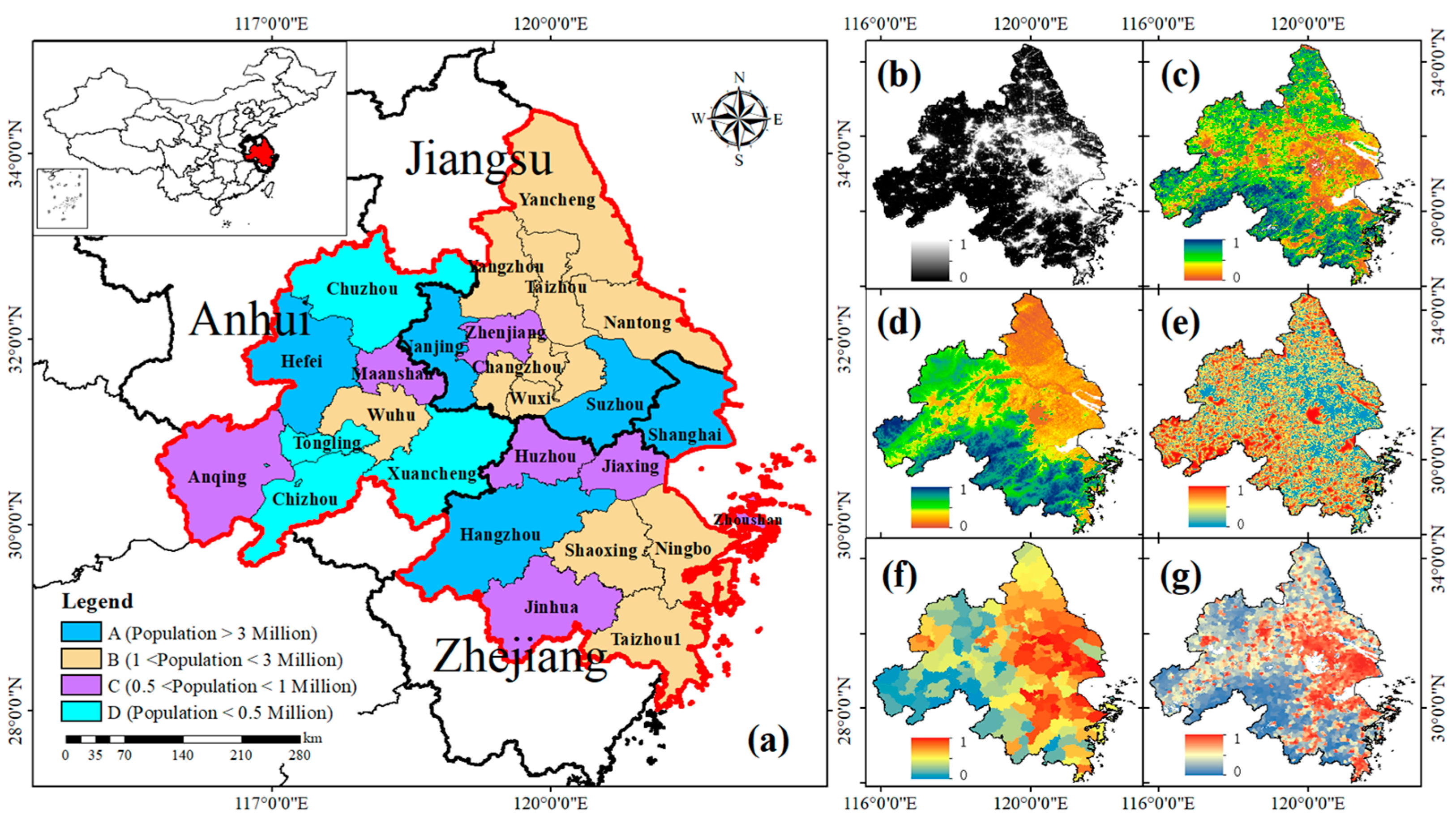
The YRD is located at 32°34′ to 29°20′ north latitude and 115°46′ to 123°25′ east longitude (Figure 1), the lower reaches of the Yangtze River, at the intersection of the river and the sea. YRD has a northern subtropical climate, and its annual average temperature is 14–18 °C. It has the highest density of river networks in China, with an average river network length of 4.8 to 6.7 kilometers per square kilometer. In this study, the YRD refers to 26 cities in Shanghai, Jiangsu, Zhejiang, and Anhui, with a total area of 213,033 km2.
2.2. Datasets and Processing
2.2.1. NTL Data Calibration
NTL data were derived from DMSP-OLS and NPP-VIIRS with spatial resolution at 30 arc-seconds and 15 arc-seconds. Version 4 DMSP-OLS data from the National Oceanic and Atmospheric Administration’s National Geophysical Data Center (NOAA/NGDC) were the annual cloud-free composites from four satellites (F14, 2000–2003; F15, 2003–2005; F16, 2005–2009; and F18, 2010–2013). Day/Night Band (DNB) of NPP-VIIRS were the annual average light data (2013–2020) from NOAA/NGDC. In addition to basic background noise (i.e., fire, gas, burning, and volcanoes; NPP VIIRS > 0.3 × 10⁻⁹ W∙cm−2∙sr−1) elimination [44], data calibration was conducted in sequential analysis by combining the datasets interlinkage.
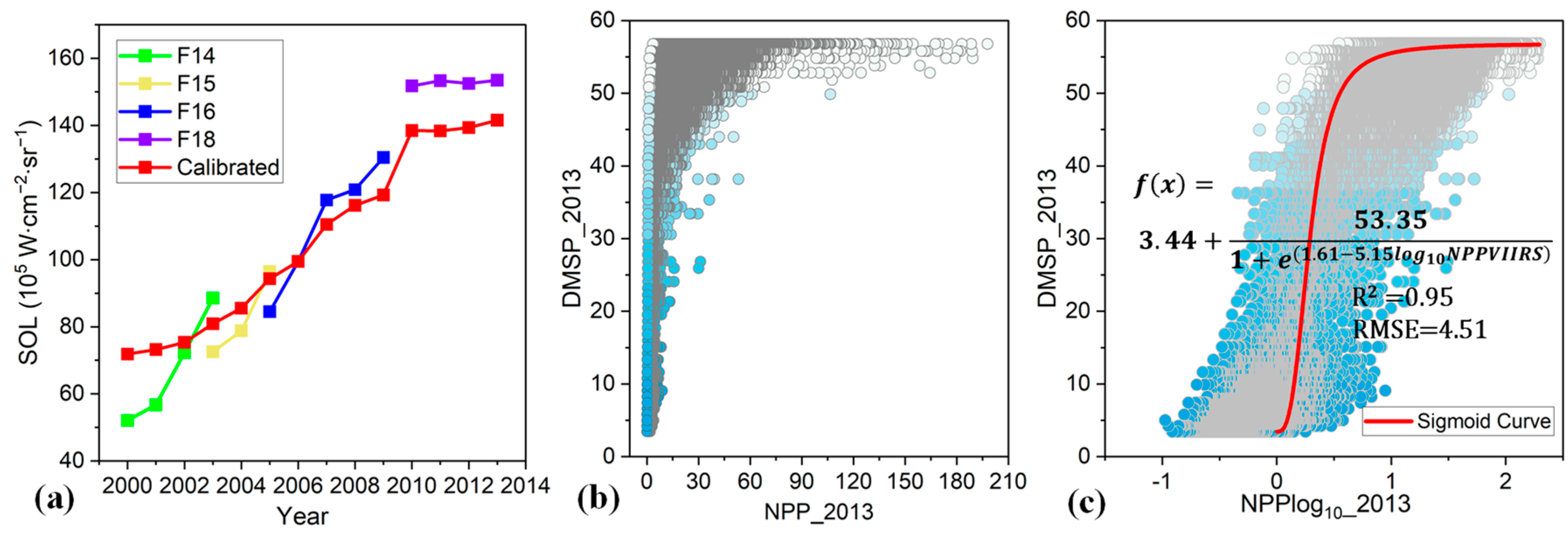
Data calibration involved the inner-calibration of DMSP-OLS with different satellites and data assimilation between DMSP-OLS and NPP-VIIRS. In the inter-calibration, a vicarious site was selected to provide calibration samples [20]. NTL data in 2007 were set as the reference, and then a power function [45] was applied to calibrate the DMSP-OLS data of the remaining years. In data assimilation, by calculating the coefficient of variation (CV) for the all the pixels in the data of DMSP-OLS and NPP-VIIRS from 2000 to 2020, a vicarious site was selected with a CV value lower than 0.2. Then an intersection operation was made between the radiation-stable areas of DMSP-OLS and NPP-VIIRS to obtain the stable pixels both spatially and temporally. Pixels in the intersection constituted the vicarious site. A logarithmic transformation was performed to adjust the range of the NPP-VIIRS data to be comparable with the DMSP-OLS data [19]. Finally, a sigmoid function was chosen as the logistic regression method for conducting data assimilation.
Data calibration of DMSP-OLS from different satellites can make the SOL values of the same year propinquities (Figure 2a). Original DMSP OLS data showed basically no relationship with NPP-VIIRS data (Figure 2b), but logarithmically transforming the NPP-VIIRS data presented a significant S-shaped distribution, performing a high R2 at 0.95 with DMSP-OLS (Figure 2c), which allows for constructing a mathematical expression to achieve the assimilation. Thus, the sigmoid model constructed in 2013 was applied to the remaining calibrated DMSP-OLS data and NPP-VIIRS data.
2.2.2. MODIS Data and Preprocessing
The MODIS surface reflectance data from 2000 to 2020 were all derived from the Terra satellite in the Earth Observation System (EOS) of the United States, with a time resolution of 8 days and a spatial resolution of 500 m. MODIS Reprojection Tool (MRT) software was used to process the original MOD09A1 data products by performing functions such as batch splicing, projection conversion, and data-format conversion. NDVI calculated by the near-infrared band (Band2) and visible-light band (Band1) of the processed MODIS surface reflectance was then filtered by the Savitzky–Golay (S–G) method to smooth the NDVI time series data. To further eliminate cloud cover, atmosphere, sun elevation, and phenology factors, this study used the maximum value composites (MVC) [46] to synthesize the NDVI at 46 time points per year. Based on the year’s maximum value of MODIS NDVI, the dimidiate pixel model was applied to calculate the MODIS FVC of the study area [47].
2.2.3. Auxiliary Data of Driving Factors
Factors in this study represented the influence of economic and physical aspects, proximity, and meteorology. Details of auxiliary data are shown in Table 1. GDP and population were derived from the NASA Socioeconomic Data and Applications Center (SEDAC) (https://sedac.ciesin.columbia.edu/, accessed on 24 December 2021). GDP in 2019 was derived from county-level statistics from the statistical yearbooks of Zhejiang, Shanghai, Jiangsu, and Anhui and was converted to raster data with spatial resolution the same as data in SEDAC. Slope (SLP) and elevation (ELV) were extracted from SRTM3 DEM data from CGIAR Consortium for Spatial Information (CGIAR-CSI) (https://srtm.csi.cgiar.org/srtmdata/, accessed on 24 December 2021). DSR is the Euclidean distance to the main road (including motorway and primary and secondary roads) of the OpenStreetMap (OSM) data downloaded from GEOFABRIK (http://www.geofabrik.de/, accessed on 24 December 2021). Road network density (RND) was calculated by using the sum length of the road within the county scale of the study area. Meteorological data, including daily maximum temperature, daily minimum temperature, and daily precipitation, were obtained from the National Meteorological Center of the China Meteorological Administration (NMCCMA) (http://www.cma.gov.cn/en2014/, accessed on 24 December 2021). Annual average temperature (TEM) was calculated based on the daily maximum temperature and daily minimum temperature. PRE is the cumulative calculation of the daily precipitation in a year. Images used in this study were all resampled to 500 m for unified processing.
3. Methods
3.1. Change Analysis of Urbanization Patterns
3.1.1. NISI and Built-Up Area Mapping
The NISI, proposed to integrate the DMSP-OLS data and MODIS NDVI for mapping ISA distribution [48], has proved to be effective in reflecting urban development. In this study, the NISI was tested to conduct urban dynamics by evaluating the intensity tendency and identifying built-up area distribution. Formulas were calculated as follows:
where , , …, and are the multitemporal MODIS NDVI images acquired from 2000 to 2020. is obtained based on the preprocessed MODIS NDVI by using the Maximum Value Composite (MVC) method. represents the normalized data of annual synthesized NTL data.
A few methods are available to directly extract built-up area information from NTL images, including an empirical thresholding technique, a thresholding technique based on mutation detection, clustering thresholding segmentation, and a statistics method with ancillary data [49]. Single threshold definition for built-up area extraction on a large scale is difficult due to the regional variation in physical environment and socioeconomic development. In this study, a K-means clustering algorithm based on the NISI was applied to extract the built-up area distribution. Statistical data (2013–2019) derived from the Ministry of Housing and Urban-Rural Development of the People’s Republic of China (MOHURD) were set as the referenced data to validate the extracted area. The determination coefficient (R2) [50] and RMSE [51] were used to evaluate the accuracy of area extraction.
3.1.2. Urbanization Intensity Tendency
Rather than classifying images into discrete land-cover types based on limited temporal snapshots, utilizing the entire time series allows urban changes over time to be easily assessed [52]. This study applied a linear regression model to calculate the NISI intensity tendency by minimizing the sum-of-squares errors [47]. The intensity tendency was the slope of the fit line after the least-squares regression of the pixel’s multiyear value, meaning the NISI interannual variability. F test was used to test the significance of variability. Formulas are as follows:
In Formula (3), the slope indicates the intensity tendency, n denotes the total number of years, i represents the ith year, and represents the value in the ith year. A positive variability represents an increasing trend or a decrease. In Formula (4), the sum of the squared errors is , the explained sum of squares is , and are the average value and regression value of NISI, respectively, and i is the year (i = 1, 2, …, n).
Hotspot analysis was performed to delineate the spatial cluster of urbanization level in the YRD based on the Getis–Ord Gi* statistic, using a fixed distance band [53]. The Getis–Ord Gi* statistic has been widely adopted to analyze biological habitat [54], epidemic disease [55], and crime [56] to identify the significant spatial clusters of high values (hotspots) and low values (cold spots). It compares the value of a variable in a given pixel and its neighboring pixel to all pixels within the analysis field in order to measure the intensity of clustering. To generate a Gi* score for a given pixel, the sum of a pixel and its neighbors is then compared proportionally to the sum of all pixels. The formula is as follows:
where is the magnitude of the NISI intensity tendency at location j, and is the averaged magnitude over all the pixels n. is the spatial weight value between the administrative pixel i and j, whose value equals either 1 or 0 defined by the distance between i and j [44].
3.2. Geographical Detectors
The geographical detector is a spatial statistical method used to test the relationships between geographical phenomena and their potential driving factors [30]. The basic idea of the model is to test the association between the explanatory variables and the dependent variable through the consistency of their spatial distribution [57]. The geographical detector includes four detectors: the factor detector, risk detector, ecology detector, and interaction detector. This study used the factor detector and the interaction detector to explore the driving mechanism.
The factor detector is used to detect the explanatory power of the factor for the dependent variable by calculating the relationship between the variances within sum of squares and the total sum of squares. The formula [58,59] is calculated as follows:
where L is the number of strata of the potential factors; and N are the number of grid element of stratum h and the whole region, respectively; and and are the variances of the urban area in the stratum h and the whole region, respectively. The greater the value of q, the greater the influence of the factor is.
The interaction detector aims to identify the interaction impact between two different factors by measuring the q-value of variables working together. For example, the interaction between factors M and N has five interactive results [60]:
- (1)
- Nonlinear-weaken: q(M∩N) < Min(q(M), q(N));
- (2)
- Uni-enhance/weaken: Min(q(M), q(N)) < q(M∩N) < Max(q(M), q(N));
- (3)
- Bi-enhance: Max (q(M), q(N)) < q(M∩N) < (q(M) + q(N));
- (4)
- Independent: q(M∩N) = q(M) + q(N);
- (5)
- Nonlinear-enhance: q(M∩N) > (q(M) +q(N));
where ∩ denotes the interaction between factors M and N.
3.3. Evaluation of Ecological Stress
Understanding the dynamics and spatial structure of object shape is a first step toward finding solutions to environmental problems [61]. In this study, the stress of urbanization on urban ecology mainly manifests itself in two ways: internal pressure and external pressure. External pressure was measured by using the morphological pattern changes of built-up areas during the process of occupation on other types of land resources. Internal pressure refers to the synchronous dynamic response of FVC to NISI.
FD and compactness can reflect the spatial concentration and diffusion of the structure, and scale-free problems will be readily resolved. For an object, only the index with non-integer value can accurately reflect its irregularity and complexity. FD is a representation of the dependence of the local features on the whole system. It is an important index for measuring the complexity and irregularity of an object or fractal, and it is a parameter to describe the degree of self-similarity of fractals quantitatively. Compactness in space with the same projected area has different plane shapes, reflecting the different degree of compactness of its spatial distribution, which can be used as an indicator of the compactness and fullness of urban forms [62]. In this study, a method based on the circumference was chosen to calculate the compactness of the geometrical shape of built-up areas. Indexes [63,64] are defined as follows:
where FDit, Cit, Pit, and represent the FD, compactness, perimeter, and size of the built-up area patches, respectively, of the ith patch in year t. FD has a value range of 1–2. Generally, the complexity of the urban form is positively correlated with FD, and the compactness of the circle is used as the metric. The greater the compactness value, the more compact the shape; conversely, the lower the value, the worse the shape compactness.
4. Results
4.1. Spatiotemporal Evolution of Urbanization
4.1.1. Evaluation of the Integrated NISI
NISI was calculated by integrating the assimilated NTL data and the processed MODIS NDVI. Image pixels of 2013 in three different directions in Hangzhou were selected to verify the spectral changes before and after data conversion. There was a great discrepancy between the original data of DMSP-OLS and those of NPP-VIIRS, due to the drawbacks of blooming effects from the near-infrared band in different sensors (Figure 3). After data assimilation, these two types showed data-distribution changes in three directions. The curve distribution shows that assimilation was better in the center of the city, and the value of some assimilated pixels in the city’s fringe area was overestimated, resulting in the SOL of NPP-VIIRS being magnified. Assimilated NTL data enhance the continuity of the time series but simultaneously cause data “saturation” of the city center compared to the original NPP-VIIRS. NISI combines the characteristics of lightness and vegetation indexes, allowing data distribution to become gradually synchronized with the original NPP-VIIRS. On the basis of almost unchanged data structure, NISI reduced light saturation and enhanced the ability in urban analysis, as with the original NPP-VIIRS data.
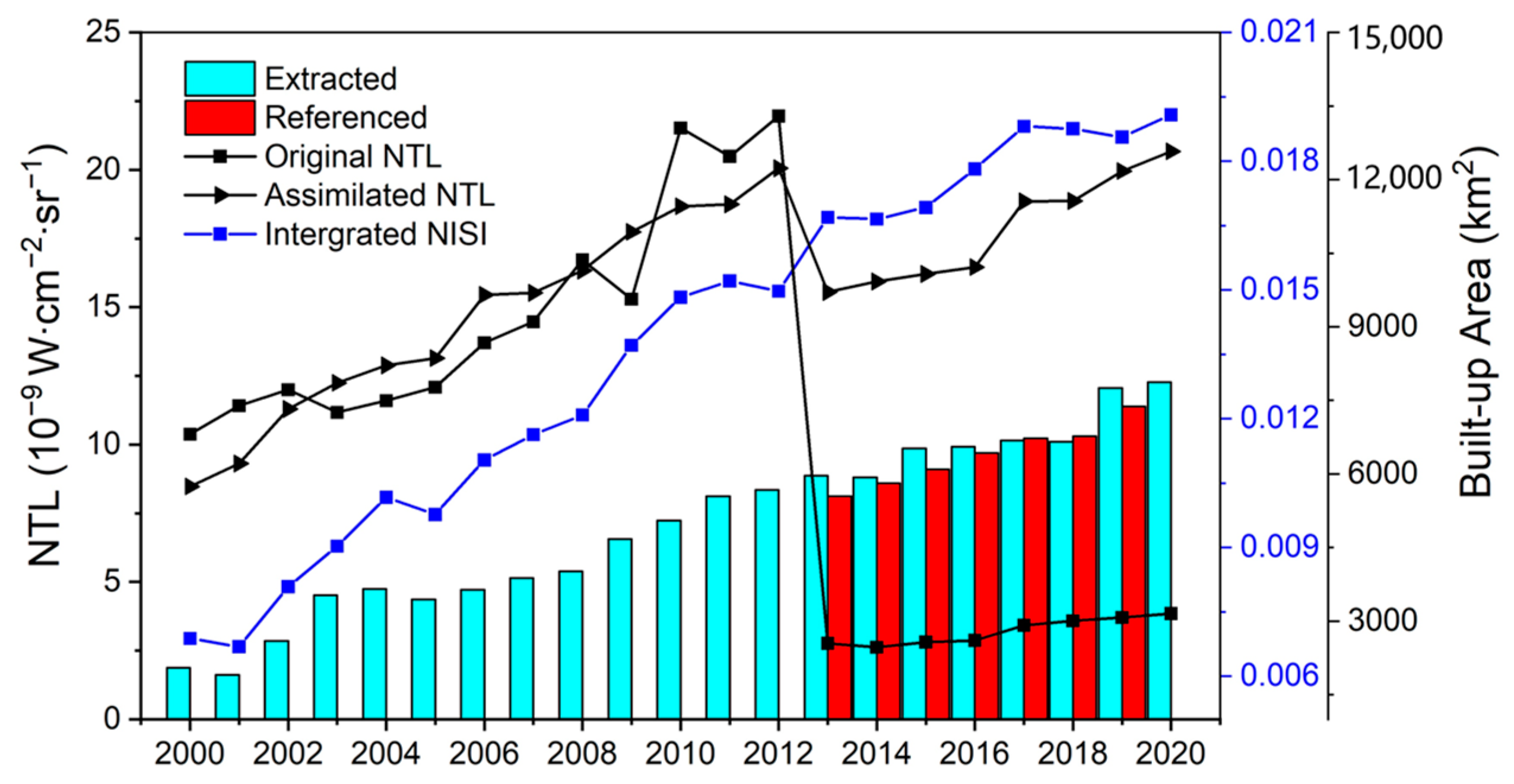
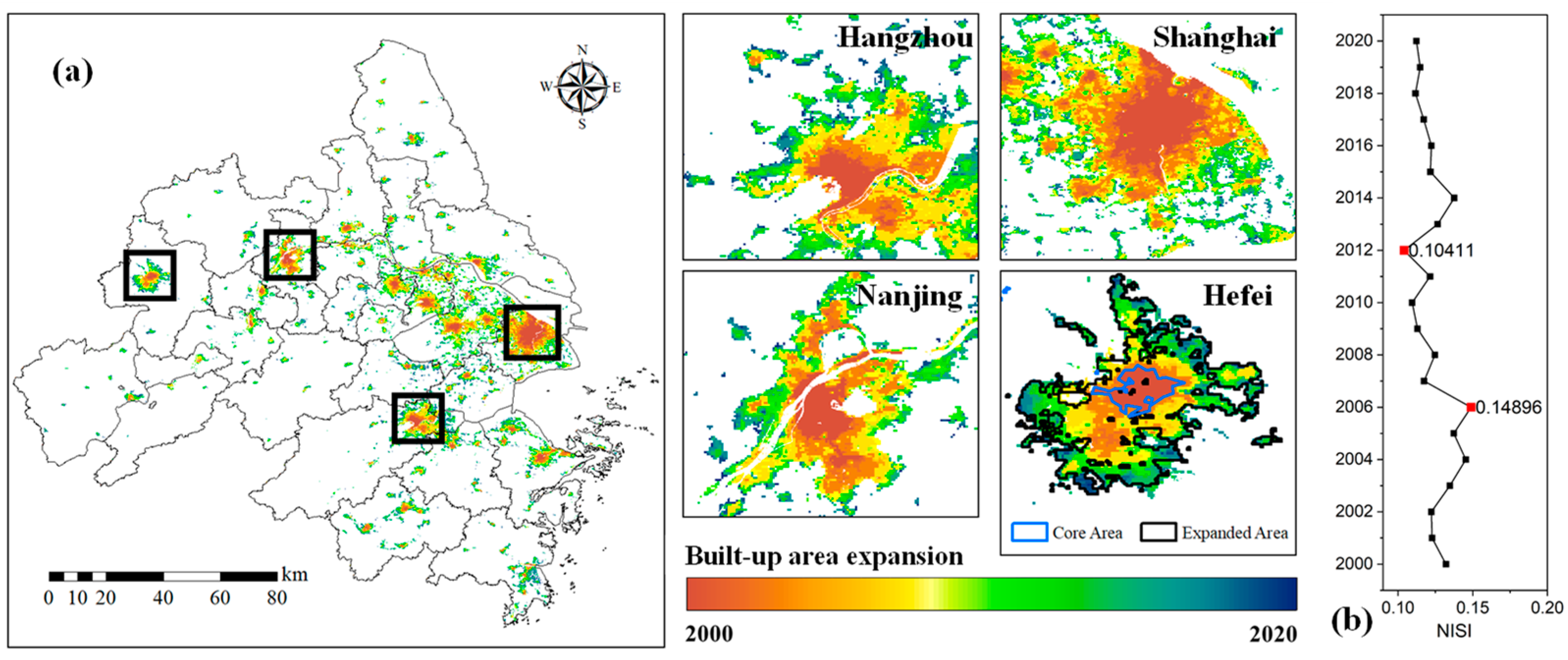
The mean value of the original NTL and the assimilated NTL shows that data assimilation can largely decrease the discontinuity of DMSP-OLS and NPP-VIIRS (Figure 4). NISI could nearly eliminate the impact of different sensors and combined the datasets interlinkage. With a high degree of pixel discrimination from the inside to the outside, NISI ingeniously reduces the light “saturation” effect to make data comparable on the pixel scale. Results of the reclassified built-up area showed a high R2 at 0.85 with the referenced area from 2013 to 2019, and low RMSE at 177.84 km2. From 2053.5 to 7872.5 km2, the built-up area in the YRD during the past two decades had an annual growth of 277.1 km2. The steady growth trend and extraction accuracy of built-up areas show that NISI can be applied to urban mapping accurately while enhancing the data continuity, which can be considered a feasible method for long-term urban detection.
4.1.2. Intensity Tendency and Hotspot Analysis
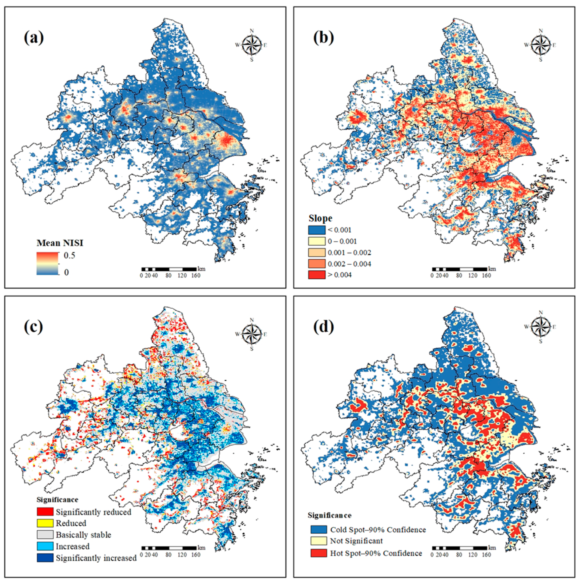
The mean NISI (Figure 5a) revealed the distribution of urbanization intensity from 2000 to 2020. The even enhancement of divergence in the city center and its marginal boundaries reflects a decreasing trend from the core to the periphery. The NISI slope of interannual change obviously revealed the spatial variation patterns, as shown in Figure 5b. Intensity variation in the built-up area’s periphery and part of the city’s core area remained relatively stable or even showed a slight decrease. Extremely and substantially increasing behaviors of the NISI slope were mainly concentrated in the middle region between the city core and the fringe area. Significant reduction and increase accounted for 10.6% and 34.2% in the slope of 62.5% decrease and 37.5% increase, respectively (Figure 5c). Considering the NISI slope, areas with drastic changes are more significant than areas with a small NISI slope appearing basically stable. Significant reduction is the case for most first-tier city centers, such as Shanghai, Suzhou, Nanjing, Hangzhou, and Hefei, while the significant increase is manifested in the periphery of these areas. Regional development is first associated with a rapid increasing intensity in the city center, until urbanization intensity saturation. Then, the rapidly increasing intensity spills over, thus accelerating the development of the surrounding suburbs and countryside in terms of both built-up area and urbanization intensity. This is roughly consistent with the research of Yu et al. [44]. Hotspot analysis with 90% confidence based on the NISI slope showed the significant spatial clusters of high values (hotspots) and low values (cold spots) (Figure 5d). Heterogeneity of a “cold to hot” and a “hot to cold” distribution could be diagnosed.
In view of the trend of economic development, the intensity of urbanization should also increase with the gradual increase of economic strength. During the study period, urbanization intensity of all 26 administrative regions increased, but not all pixels within the region were positive. Statistics showed that the built-up area of some cities has been almost stable in recent years, which means that outward expansion is inevitably accompanied by an internal decrease. Results revealed that the more densely populated areas are the first to reach the peak of urbanization in the core area, while for the expansion area, the opposite is the case.
4.2. Driving Mechanism of Urbanization
Biophysical factors and human activities affect urbanization, with drivers varying across regions over time [30]. Due to comprehensive influences, the sensitivity of factors to urbanization is constantly changing over time and space. In this study, NISI and driving factors from 2000 to 2020 were set as the independent and dependent variables applied to analyze the driving mechanism. Results are presented in Figure 6.
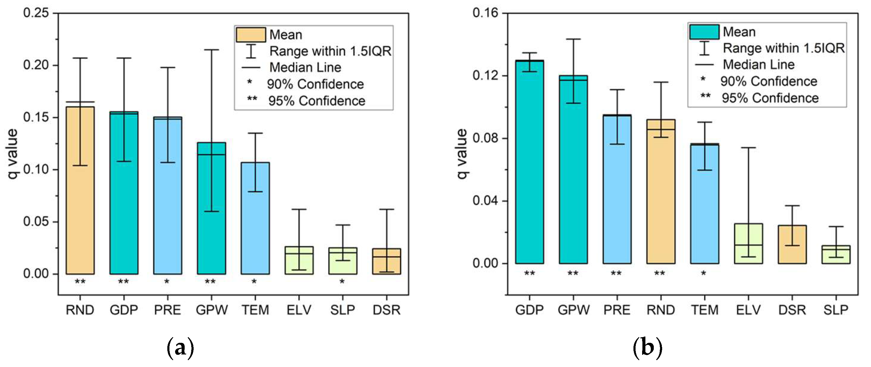
From the perspective of different periods (2000–2005, 2005–2010, 2010–2015, and 2015–2020) (Figure 6a), factors are ordered by mean q-values: RND (0.1603) > GDP (0.1555) > PRE (0.1505) > GPW (0.1260) > TEM (0.1070) > ELV (0.0263) > SLP (0.0252) > DSR (0.0242). In particular, the influence of RND is more prominent than economic factors in this study. The distribution and density of roads are determined by human activity, which is understandably one of the main vital factors of urbanization. Economic factors are primary for urban development, making it reasonable that GDP and GPW were identified as the main driving factors. Compared with other factors, the sensitivity of urbanization to GPW varies most in different periods. Meteorological factor PRE and TEM with high q-values, but not significant as economic factors, were more significant than proximity factor DSR and physical factors ELV and SLP. Their interpretation as a direct impact on urbanization is yet to be understood, while it is acceptable for meteorological data to influence urbanization development by imaging vegetation conditions or other land use. From a regional perspective of areas with different population levels (A, B, C, and D) (Figure 6b), factors were ranked with mean q-values: GDP (0.1293) > GPW (0.1201) > PRE (0.094)> RND (0.092) > TEM (0.076) > ELV (0.026) > SLP (0.024) > DSR (0.011). GDP, GPW, PRE, and RND have no obvious differences or variability in regions with different population levels. They all have significant effects on urbanization. Compared with GDP, the variation of GPW is greater; that is, the role of population in urbanization is more volatile in different regions. Population is important in driving economic development and urbanization, but not always the most important factor on a total regional scale. Results showed that the role of GDP is weaker than that of GPW only in the most populated regions. As the same proximity factor, the sensitivity of urbanization to DSR is much lower than RND. In fact, the higher the density of road network in areas with faster economic development, the smaller the distance to roads. For pixels with lower DSR, the intensity of urbanization is greater. At the same time, this study also confirmed that physical factors have a weak influence on urbanization.
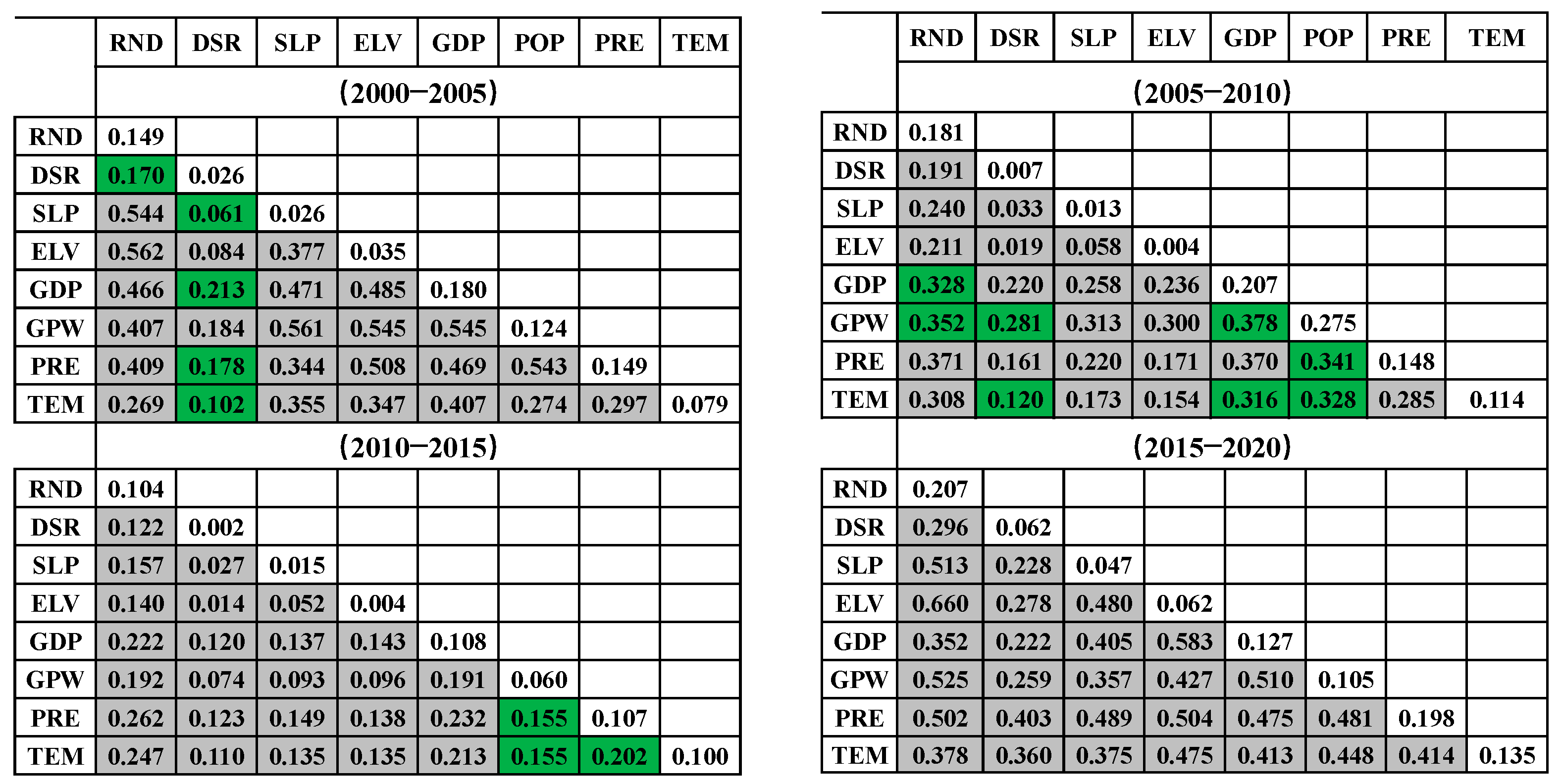
Interaction detector can quantify the influence of factors’ superposition on driving urbanization (Figure 7). The value on the diagonal line represents the original factors’ q-values, and the others are interaction results with factors superimposing.
Socioeconomic driving factors were continuously the main contributors to urbanization in different periods over the study area. The interactive effect showed the pairwise factors with two situations, bi-enhance effect and nonlinear-enhance effect, having enhanced the explanatory power of urbanization. In the first period, except for the bi-enhance effect produced by the proximity factors superimposed on other factors, superposition of remaining factors produced a nonlinear-enhance effect, explaining the relative independence. Socioeconomic and proximity factors presented a bi-enhance effect when they were superposed with the socioeconomic and meteorological factors during the second time period. While superposition of physical factors with other factors will not produce collinear effects, SLP and ELV are also not sensitive to supplementing urbanization intensity changes.
4.3. Stress on Urban Ecology
4.3.1. Urban External Structure Change
NISI dynamics revealed the urbanization intensity on the pixel scale, but the characteristics of spatiotemporal changes on the regional scale are still an unsolved problem. It is difficult to capture the spatial evolution of built-up area expansion in a short time interval, both in the inner and outer area. In order to quantify the variation effect of expansion, built-up regions of unchanged area and enlarged area were defined as the core area and expanded area, respectively. Built-up area expansion presents a spatial distribution of urbanization (Figure 8).
With the rapid development of smart cities, improving citizens’ sense of happiness is regarded as the fundamental purpose of city governance. Due to socioeconomic factors and people’s continuously developing housing demands, the spatial distribution and shape of built-up areas tend to be complicated. From 2000 to 2020, there were discrepancies in the distribution of FD and compactness in the 26 districts (Figure 9). The mean value from 1.16 to 1.18 and 0.21 to 0.17 of FD and compactness showed increment and decline, respectively, illustrating that the shape of patches is becoming more complicated and less compact. It is an indirect description of the increasing fragmentation of spatial structure with rapid urban development. With the increasing complexity, the threat to ecology gradually becomes worse and more complicated. Variation of the two indictors in the 26 districts exhibits spatiotemporal heterogeneity. The difference of the 26 districts’ value in the two indicators, which gradually shrank, especially compactness, revealed that built-up areas in different regions are becoming integrated and coordinated. Increments in FD are often accompanied by a decrease in compactness, showing a counter state, which is consistent with the conclusion that compactness proved to be the exponential function of the reciprocal of the boundary dimension [39].
4.3.2. Dynamic Response of FVC to NISI
Urbanization is essentially a type of land use. Cultivated land and some urban greening spaces are the principal source of expansion in rapid development regions. This study applied the FVC derived from MODIS reflectance as the vegetation index to evaluate the impact of urbanization on urban greenness.
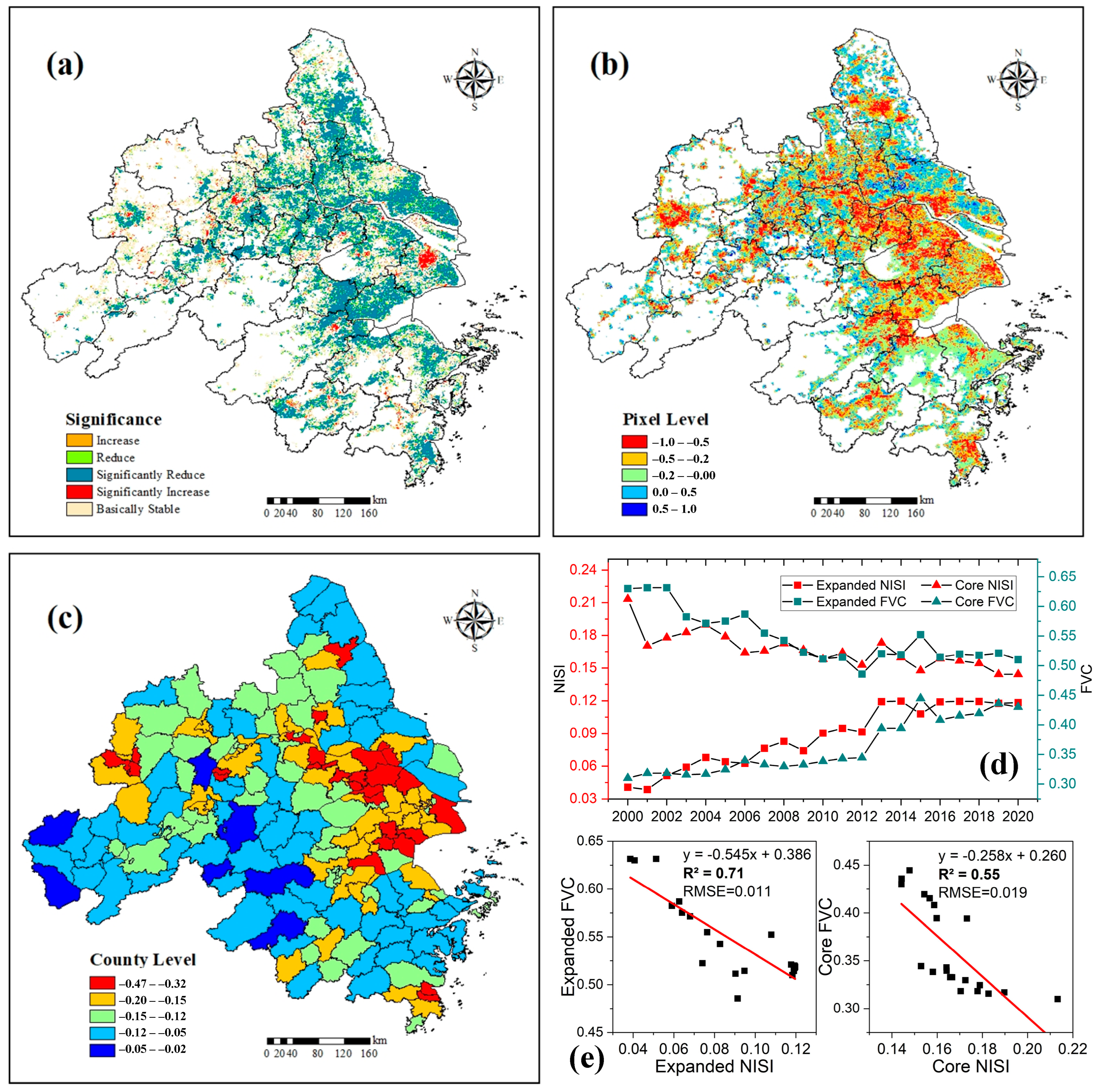
The slope of FVC from 2000 to 2020 was measured to reveal its variation (Figure 10a). The relationship between NISI and FVC was measured by Pearson correlation analysis (Figure 10b,c). Interannual variability of FVC in the past two decades showed a significant decrease in the periphery of expanded built-up area. As for the relatively stable core area, urbanization changed with a significant increase. This is in accordance with expansion density “saturation” and apparent tending declination. The Pearson correlation coefficient of NISI and FVC in the pixel scale can explicitly indicate the severe distribution of occupied vegetation by urbanization. The negative coefficient accounted for 63.4% of the total area, and the most seriously affected, with a value from −1 to −0.5, had a proportion of 16.7%. This negative function results from the occupation by urbanization of green land. Urbanization can supervise the green coverage rate in some areas. On the one hand, these areas have been gradually developed into built-up areas and green land from the initial bare land or other land use. On the other hand, more attention is paid to the importance of green land in the burgeoning process, which slows down the speed of urbanization and improves the status of urban greenness. This can be seen from the decrease of urbanization intensity and the slight negative impact on FVC in the city center. At the national level (Figure 10c), influence on urbanization in Shanghai, Jiaxing, Suzhou, and Hefei was the most grievous. In this study, more than half of the negative effects (63.4%) can be attributed to the fact that green land is the main resource for expansion. Therefore, at the national level, all negative correlations can be understood as a phenomenon of rapid urbanization. That is, the amount of vegetation decreases, and cities expand. Moreover, the stronger this negative effect is, the more serious the urbanization will be. The mean FVC and mean NISI from 2000 to 2020 in the core and expanded area showed an increasing tendency (Figure 10d). NISI increase was simultaneously with the FVC declination. The FVC decrement in the expanded area was mostly due to the occupation of built-up area, while the FVC increment in the core area had a great influence on green development policies. As the urbanization of the central city becomes saturated, urban greenness cover is enhanced. FVC in the city center is less vulnerable to urbanization than the expanded area (Figure 10e).
5. Discussion
NTL data can effectively reflect the latest situation of human activities and economic development. Compared with general remote-sensing data, the prominent merit of NTL lies in its data availability and wide application at a regional scale. The cross-sensor of NTL causes data discontinuity in long-term detection. Logarithmic transformation effectively suppresses the sharp NPP-VIIRS radiance fluctuations within city centers and strengthens the NPP-VIIRS radiance variance, enhancing the data continuity of DMSP-OLS and NPP-VIIRS. Urban indexes based on NTL data have been studied, but few are directly used to detect the long-term urbanization process. In this study, NISI was confirmed to further improve the potentiality of understanding urbanization. Results revealed that urbanization in the YRD occurred simultaneously inside and outside. NISI slope can nearly capture the change in urbanization intensity in the city center with a slight increment that is accompanied with area decrease. The National Forest City Development Plan (2018–2025) indicated that an agglomeration of six state-level forest cities would be constructed in China by 2020, including the YRD. As a region of rapid economic development, the built-up area in Shanghai showed an obvious increment in the initial stage and gradually became stable in recent years, with obvious growth in its urban forest cover rate. This phenomenon can also be traced in Hangzhou, Hefei, Nanjing, and some other new first-tier cities. At the same time, NISI can enhance the edge contrast of ISA and other land types, which increased the credibility of built-up area mapping.
The driving effect of factors on urbanization fluctuates more strongly in time periods than that of different population regions in space. The driving mechanism in this study demonstrated that GDP and population are critical factors in driving urbanization. Economic development promoted the migration process from rural settlements to cities. Then, population growth in cities gradually increased housing demand, which resulted in the expansion of built-up areas and complexity in the shape and structure. At the same time, it was found that road network density became a more prominent factor for urban construction. As the infrastructure of urbanization development, the road network is of great significance in a practical sense. However, studies on the influence of urban development on climate mostly focuses on the urban microclimate. The relationship between large-scale urbanization and climate change is unclear. Elevation and slope showed little effect on expansion. Urbanization-intensity variation is seemingly mostly dependent on human interference. Furthermore, high-altitude and steep areas are less likely to be developed, because more money is needed to construct built-up areas in these regions compared to flat areas. The interaction factor can effectively identify the influence of factor superposition. The bidirectional enhancement of interactions between economic factors rather than nonlinear enhancement also indicated the possibility of collinearity between factors.
Urbanization is the comprehensive result of human interference. Impervious infrastructure was assumed not to exist in initial natural states; thus, some researchers regard urban analysis as a way to evaluate the pressure of urbanization on the ecosystem [35]. Especially since the reform and opening-up in 1978, China’s urbanization has been through several stages [65]. The increment of built-up area is the most direct embodiment of the linear increase of ecological pressure. Changes of built-up area geometric shapes reflect the gradual complication of geometrical boundary structure. While the built-up area continues to expand outward, the gradual increase and decrease of FD and compactness not only means an increment in ecological pressure on ecology but also a complication of urban development. Complexity and inconsistency increased the difficulty of management and put forward higher requirements for the development of intelligent cities [66]. As the light brightness decreases in the city core and increases on the periphery, the direction of urbanization is shifting from the city center to the edge. It has gradually complicated the morphology and structure of built-up areas, especially for some slow-developing cities, and their urbanization development structure needs to be further adjusted. The negative correlation between urbanization and FVC indicates that vegetation loss has an intricate relationship with urban development. Green plants play an indispensable role in achieving the country’s carbon peak and carbon neutrality goals, especially in built-up areas; patterns and persistence of urban greening are particularly important. Alleviating urbanization in city centers is a strategic adjustment that can transform development. In this study, the intensity of urbanization in the city center shows a decline, which is a form of strategic adjustment and a manifestation of the fact that urban vegetation is increasingly valued. The decline in green coverage caused by urban expansion (mainly forests and cultivated land) leads to a decrease in ecological value. This study analyzed the ecological pressure caused by the change of urban shape and urban greenness in the process of urbanization from a qualitative point of view, but the specific number should also be given in future quantitative studies, as it is of great significance to the sustainable development of green cities.
With the constant renewal of society, rapid development will impose stricter requirements on urban monitoring. Long-term analysis of urbanization based on NTL data can only stay at a middle and low resolution, which is still a great challenge for urban spatiotemporal monitoring with large-scale refinement. Furthermore, one of the major problems faced by the integrated application of multisource data is the spatial consistency. The combination of datasets from different platforms will inevitably produce geometric errors. Currently, methods of geometric correction for cross-sensor data are available for some kinds of datasets, and their application scope is still limited. Moreover, it is difficult to realize the precise geometric correction for large-scale and multidimensional datasets. Furthermore, we are committed to combining some more effective ecological indicators to accurately quantify the effect of urban development on urban ecological pressure, which can help managers make more specific and reasonable plans for urban development.
6. Conclusions
By calibrating the data of DMSP-OLS and NPP-VIIRS, long-time-series-processed NTL data integrated with MODIS data were used to conduct the NISI for analysis of urbanization intensity change and impact on urban ecological stress. This study proved that the corrected NTL data combined with MODIS NDVI can improve the data continuity and reliability of long-term urban monitoring, which provides a new reference for time series urban monitoring. Urbanization dynamics in the YRD show that, accompanied by reaching saturation in the city center, urban-development gravity gradually moves to the periphery. In addition to economic factors, road network density, as an important factor reflecting urban infrastructure, needs to be considered in driving urban development. Urbanization has had a significant influence on the city’s internal social attributes and external physical structure. In the process of physical structural changes caused by urban expansion, changes in FD and compactness can eventually complicate the urban landscape structure and increase urban ecological stress. Meanwhile, variation of urbanization intensity has a great impact on urban FVC. The spatiotemporal negative correlation between urban development and urban greenness in a sizeable area and, over a long time, shows that urban development is an important factor in urban greenness disturbance. This effect in the city center is smaller than that in the expansion area, which is not only a phenomenon of the short-term degradation of vegetation caused by the occupation of land resources in the early stage but also a strategic manifestation of urban coordinated development. Urban planning and ecology protection are factors that development always pay attention to. Quantifying their patterns and mechanisms is of great significance for society sustainable development.
Author Contributions
Conceptualization, H.D. and G.Z.; data curation, M.Z.; formal analysis, M.Z. and X.L.; funding acquisition, G.Z.; investigation, F.M., L.Z., D.Z., Y.X. and Z.H.; methodology, M.Z. and X.L.; project administration, H.D. and G.Z.; resources, H.D.; software, M.Z., F.M. and X.L.; supervision, H.D. and G.Z.; writing—original draft, M.Z.; writing—review and editing, H.D. All authors have read and agreed to the published version of the manuscript.
Funding
This research was funded by National Natural Science Foundation of China (No. U1809208, 32171785), the State Key Laboratory of Subtropical Silviculture (No. ZY20180201), the Talent launching project of scientific research and development fund of Zhejiang A & F University (No. 2021LFR029), and the Key Research and Development Program of Zhejiang Province (2021C02005).
Institutional Review Board Statement
Not applicable.
Informed Consent Statement
Not applicable.
Data Availability Statement
Not applicable.
Acknowledgments
The authors are grateful to the editor and anonymous reviewers whose comments have contributed to improving the quality of this study.
Conflicts of Interest
The authors declare that they have no competing interests.
References
- Liu, Z.; Ding, M.; He, C.; Li, J.; Wu, J. The impairment of environmental sustainability due to rapid urbanization in the dryland region of northern China. Landsc. Urban Plan. 2019, 187, 165–180. [Google Scholar] [CrossRef]
- Liu, H.; Huang, B.; Gao, S.; Wang, J.; Li, R. Impacts of the evolving urban development on intra-urban surface thermal environment: Evidence from 323 Chinese cities. Sci. Total. Environ. 2021, 771, 144810. [Google Scholar]
- Yu, D.; Wei, Q.B.; Bfa, C.; Kw, D. Geographical transformations of urban sprawl: Exploring the spatial heterogeneity across cities in China 1992–2015. Cities 2019, 105. [Google Scholar] [CrossRef]
- Das, M.; Das, A. Dynamics of Urbanization and its impact on Urban Ecosystem Services (UESs): A study of a medium size town of West Bengal, Eastern India. J. Urban Manag. 2019, 8, 420–434. [Google Scholar] [CrossRef]
- Moghadam, A.S.; Soltani, A.; Parolin, B.; Alidadi, M. Analysing the space-time dynamics of urban structure change using employment density and distribution data. Cities 2018, 81, 203–213. [Google Scholar]
- He, Y.; Wang, W.; Chen, Y.; Yan, H. Assessing spatio-temporal patterns and driving force of ecosystem service value in the main urban area of Guangzhou. Sci. Rep. 2021, 11, 1–8. [Google Scholar] [CrossRef]
- Dong, Y.; Ren, Z.; Fu, Y.; Miao, Z.; Yang, R.; Sun, Y.; He, X. Recording Urban Land Dynamic and Its Effects during 2000–2019 at 15-m Resolution by Cloud Computing with Landsat Series. Remote Sens. 2020, 12, 2451. [Google Scholar] [CrossRef]
- Xu, F.; Somers, B. Unmixing-based Sentinel-2 downscaling for urban land cover mapping. ISPRS J. Photogramm. Remote Sens. 2021, 171, 133–154. [Google Scholar]
- Cao, X.; Chen, J.; Imura, H.; Higashi, O. A SVM-based method to extract urban areas from DMSP-OLS and SPOT VGT data. Remote Sens. Environ. 2009, 113, 2205–2209. [Google Scholar] [CrossRef]
- Sma, B.; Mha, C. Spatiotemporal variability of urban growth factors: A global and local perspective on the megacity of Mumbai. Int. J. Appl. Earth Obs. Geoinf. 2015, 35, 187–198. [Google Scholar]
- Zhou, Y.; Li, X.; Asrar, G.R.; Smith, S.J.; Imhoff, M. A global record of annual urban dynamics (1992–2013) from nighttime lights. Remote Sens. Environ. 2018, 219, 206–220. [Google Scholar] [CrossRef]
- Cheng, L.; Zhou, Y.; Wang, L.; Wang, S.; Du, C. An Estimate of the City Population in China using DMSP Night-Time Satellite Imagery. In Proceedings of the IEEE International Geoscience & Remote Sensing Symposium, Barcelona, Spain, 23–28 July 2007. [Google Scholar]
- Zhao, N.; Hsu, F.C.; Cao, G.; Samson, E.L. Improving accuracy of economic estimations with VIIRS DNB image products. Int. J. Remote Sens. 2017, 38, 1–20. [Google Scholar] [CrossRef]
- Chunyang, H.E.; Qun, M.A.; Tong, L.I.; Yang, Y.; Liu, Z. Spatiotemporal dynamics of electric power consumption in Chinese Mainland from 1995 to 2008 modeled using DMSP/OLS stable nighttime lights data. Acta Geogr. Sin. 2012, 22, 125–136. [Google Scholar]
- Yu, B.; Shi, K.; Hu, Y.; Huang, C.; Chen, Z.; Wu, J. Poverty Evaluation Using NPP-VIIRS Nighttime Light Composite Data at the County Level in China. IEEE J. Sel. Top. Appl. Earth Obs. Remote Sens. 2017, 8, 1217–1229. [Google Scholar] [CrossRef]
- Levin, N.; Kyba, C.C.; Zhang, Q.; de Miguel, A.S.; Román, M.O.; Li, X.; Portnov, B.A.; Molthan, A.L.; Jechow, A.; Miller, S.D.; et al. Remote sensing of night lights: A review and an outlook for the future. Remote Sens. Environ. 2020, 237, 111443. [Google Scholar] [CrossRef]
- Bennett, M.M.; Smith, L.C. Advances in using multitemporal night-time lights satellite imagery to detect, estimate, and monitor socioeconomic dynamics. Remote Sens. Environ. 2017, 192, 176–197. [Google Scholar] [CrossRef]
- Wang, J.; Roudini, S.; Hyer, E.J.; Xu, X.; Zhou, M.; Garcia, L.C.; Reid, J.S.; Peterson, D.A.; Da Silva, A.M. Detecting nighttime fire combustion phase by hybrid application of visible and infrared radiation from Suomi NPP VIIRS. Remote Sens. Environ. 2020, 237, 111466. [Google Scholar] [CrossRef]
- Zhao, M.; Zhou, Y.; Li, X.; Zhou, C.; Cheng, W.; Li, M.; Huang, K. Building a Series of Consistent Night-Time Light Data (1992–2018) in Southeast Asia by Integrating DMSP-OLS and NPP-VIIRS. IEEE Trans. Geosci. Remote Sens. 2019, 58, 1843–1856. [Google Scholar] [CrossRef]
- Ma, J.; Guo, J.; Ahmad, S.; Li, Z.; Hong, J. Constructing a New Inter-Calibration Method for DMSP-OLS and NPP-VIIRS Nighttime Light. Remote Sens. 2020, 12, 937. [Google Scholar] [CrossRef] [Green Version]
- Lu, D.; Tian, H.; Zhou, G.; Ge, H. Regional mapping of human settlements in southeastern China with multisensor remotely sensed data. Remote Sens. Environ. 2015, 112, 3668–3679. [Google Scholar] [CrossRef]
- Xiaoping, L.; Guohua, H.; Bin, A.; Xia, L.; Qian, S. A Normalized Urban Areas Composite Index (NUACI) Based on Combination of DMSP-OLS and MODIS for Mapping Impervious Surface Area. Remote Sens. 2015, 7, 17168–17189. [Google Scholar]
- Zhuo, L.; Zheng, J.; Zhang, X.; Li, J.; Liu, L. An improved method of night-time light saturation reduction based on EVI. Int. J. Remote Sens. 2015, 36, 4114–4130. [Google Scholar] [CrossRef]
- Guo, W.; Lu, D.; Kuang, W. Improving Fractional Impervious Surface Mapping Performance through Combination of DMSP-OLS and MODIS NDVI Data. Remote Sens. 2017, 9, 375. [Google Scholar] [CrossRef] [Green Version]
- Yangxiaoyue, L.; Yaping, Y.; Wenlong, J.; Ling, Y.; Xiafang, Y.; Xiaodan, Z. A New Urban Index for Expressing Inner-City Patterns Based on MODIS LST and EVI Regulated DMSP/OLS NTL. Remote Sens. 2017, 9, 777. [Google Scholar]
- Grimm, N.B.; Faeth, S.H.; Golubiewski, N.E.; Redman, C.L.; Wu, J.; Bai, X.; Briggs, J.M. Global change and the ecology of cities. Science 2008, 319, 756–760. [Google Scholar] [CrossRef] [Green Version]
- Dadashpoor, H.; Azizi, P.; Moghadasi, M. Analyzing spatial patterns, driving forces and predicting future growth scenarios for supporting sustainable urban growth: Evidence from Tabriz metropolitan area, Iran. Sustain. Cities Soc. 2019, 47, 101502. [Google Scholar] [CrossRef]
- Kaza, N. The changing urban landscape of the continental United States. Landsc. Urban Plan. 2013, 110, 74–86. [Google Scholar] [CrossRef]
- Song, W.; Li, H. Spatial pattern evolution of rural settlements from 1961 to 2030 in Tongzhou District, China. Land Use Policy 2020, 99, 105044. [Google Scholar] [CrossRef]
- Zhou, Y.; Li, X.; Liu, Y. Land use change and driving factors in rural China during the period 1995–2015. Land Use Policy 2020, 99, 105048. [Google Scholar] [CrossRef]
- Liu, Y.; Cao, X.; Li, T. Identifying Driving Forces of Built-Up Land Expansion Based on the Geographical Detector: A Case Study of Pearl River Delta Urban Agglomeration. Int. J. Environ. Res. Public Health 2020, 17, 1759. [Google Scholar] [CrossRef] [PubMed] [Green Version]
- Wang, J.; Li, X.; Christakos, G.; Liao, Y.; Zhang, T.; Gu, X.; Zheng, X. Geographical Detectors-Based Health Risk Assessment and its Application in the Neural Tube Defects Study of the Heshun Region, China. Int. J. Geogr. Inf. Sci. 2010, 24, 107–127. [Google Scholar] [CrossRef]
- Wang, J.; Xu, C. Geodetector: Principle and prospective. Acta Geogr. Sin. 2017, 72, 116–134. [Google Scholar]
- Chen, W.; Yan, D.; Sun, W. Analyzing the patterns and processes of new urbanization development in the Yangtze River Delta. Geogr. Res. 2015, 34, 397–406. [Google Scholar]
- Lin, M.; Lin, T.; Jones, L.; Liu, X.; Xing, L.; Sui, J.; Zhang, J.; Ye, H.; Liu, Y.; Zhang, G.; et al. Quantitatively Assessing Ecological Stress of Urbanization on Natural Ecosystems by Using a Landscape-Adjacency Index. Remote Sens. 2021, 13, 1352. [Google Scholar] [CrossRef]
- Liang, Y.; Liu, L. Simulating land-use change and its effect on biodiversity conservation in a watershed in northwest China. Ecosyst. Health Sustain. 2017, 3. [Google Scholar] [CrossRef] [Green Version]
- Jevric, M.; Romanovich, M. Fractal Dimensions of Urban Border as a Criterion for Space Management. Procedia Eng. 2016, 165, 1478–1482. [Google Scholar] [CrossRef]
- Yuan, H.; He, Y.; Zhou, J.; Li, Y.; Cui, X.; Shen, Z. Research on Compactness Ratio Model of Urban Underground Space and Compact Development Mechanism of Rail Transit Station Affected Area. Sustain. Cities Soc. 2020, 55, 102043. [Google Scholar] [CrossRef]
- Chen, Y. Derivation of the functional relations between fractal dimension of and shape indices of urban form. Comput. Environ. Urban Syst. 2011, 35, 442–451. [Google Scholar] [CrossRef]
- Deng, X.; Huang, J.; Rozelle, S.; Zhang, J.; Li, Z. Impact of urbanization on cultivated land changes in China. Land Use Policy 2015, 45, 1–7. [Google Scholar] [CrossRef]
- Mu, X.; Hu, M.; Song, W.; Ruan, G.; Yan, G. Fractional Vegetation Cover. In Advanced Remote Sensing; Academic Press: Cambridge, MA, USA, 2012; pp. 415–438. [Google Scholar]
- Yao, R.; Cao, J.; Wang, L.; Zhang, W.; Wu, X. Urbanization effects on vegetation cover in major African cities during 2001–2017. Int. J. Appl. Earth Obs. Geoinf. 2019, 75, 44–53. [Google Scholar] [CrossRef]
- Carrus, G.; Scopelliti, M.; Lafortezza, R.; Colangelo, G.; Ferrini, F.; Salbitano, F.; Agrimi, M.; Portoghesi, L.; Semenzato, P.; Sanesi, G. Go greener, feel better? The positive effects of biodiversity on the well-being of individuals visiting urban and peri-urban green areas. Landsc. Urban Plan. 2015, 134, 221–228. [Google Scholar] [CrossRef]
- Yu, M.; Guo, S.; Guan, Y.; Cai, D.; Zhang, C.; Fraedrich, K.; Liao, Z.; Zhang, X.; Tian, Z. Spatiotemporal Heterogeneity Analysis of Yangtze River Delta Urban Agglomeration: Evidence from Nighttime Light Data (2001–2019). Remote Sens. 2021, 13, 1235. [Google Scholar] [CrossRef]
- Shao, X.; Cao, C.; Zhang, B.; Shi, Q.; Elvidge, C.; Von Hendy, M. Radiometric calibration of DMSP-OLS sensor using VIIRS day/night band. In Proceedings of the Earth Observing Missions and Sensors: Development, Implementation, and Characterization III, SPIE Asia-Pacific Remote Sensing, Beijing, China, 19 November 2014; Volume 9264. 92640A. [Google Scholar]
- Li, J.; Zhang, J.; Liu, C.; Yang, X. Spatiotemporal Variation of Vegetation Coverage in Recent 16 Years in the Border Region of China, Laos, and Myanmar Based on MODIS-NDVI. Sci. Silvae Sin. 2019, 55, 9–18. [Google Scholar]
- Liu, H.; Li, X.; Mao, F.; Zhang, M.; Zhu, D.; He, S.; Huang, Z.; Du, H. Spatiotemporal Evolution of Fractional Vegetation Cover and Its Response to Climate Change Based on MODIS Data in the Subtropical Region of China. Remote Sens. 2021, 13, 913. [Google Scholar] [CrossRef]
- Guo, W.; Lu, D.; Wu, Y.; Zhang, J. Mapping Impervious Surface Distribution with Integration of SNNP VIIRS-DNB and MODIS NDVI Data. Remote Sens. 2015, 7, 12459–12477. [Google Scholar] [CrossRef] [Green Version]
- Chang, S.; Wang, J.; Zhang, F.; Niu, L.; Wang, Y. A study of the impacts of urban expansion on vegetation primary productivity levels in the Jing-Jin-Ji region, based on nighttime light data. J. Clean. Prod. 2020, 263, 121490. [Google Scholar] [CrossRef]
- Li, Y.; Han, N.; Li, X.; Du, H.; Mao, F.; Cui, L.; Liu, T.; Xing, L. Spatiotemporal Estimation of Bamboo Forest Aboveground Carbon Storage Based on Landsat Data in Zhejiang, China. Remote Sens. 2018, 10, 898. [Google Scholar] [CrossRef] [Green Version]
- Zhang, M.; Du, H.; Mao, F.; Zhou, G.; Li, X.; Dong, L.; Zheng, J.; Zhu, D.E.; Liu, H.; Huang, Z.; et al. Spatiotemporal Evolution of Urban Expansion Using Landsat Time Series Data and Assessment of Its Influences on Forests. Int. J. Geo-Inf. 2020, 9, 64. [Google Scholar] [CrossRef] [Green Version]
- Lu, Y.; Coops, N.C.; Hermosilla, T. Estimating urban vegetation fraction across 25 cities in pan-Pacific using Landsat time series data. Isprs J. Photogramm. Remote Sens. 2017, 126, 11–23. [Google Scholar] [CrossRef]
- Jana, M.; Sar, N. Modeling of hotspot detection using cluster outlier analysis and Getis-Ord Gi* statistic of educational development in upper-primary level, India. Modeling Earth Syst. Environ. 2016, 2, 60. [Google Scholar] [CrossRef] [Green Version]
- Cleasby, I.R.; Owen, E.; Wilson, L.; Wakefield, E.D.; O’Connell, P.; Bolton, M. Identifying important at-sea areas for seabirds using species distribution models and hotspot mapping. Biol. Conserv. 2020, 241, 108375. [Google Scholar] [CrossRef]
- Gwitira, I.; Murwira, A.; Zengeya, F.M.; Shekede, M. Application of GIS to predict malaria hotspots based on Anopheles arabiensis habitat suitability in Southern Africa. Int. J. Appl. Earth Obs. Geoinf. 2018, 64, 12–21. [Google Scholar] [CrossRef]
- Ratcliffe, J.H. Damned If You Don’t, Damned If You Do: Crime Mapping and its Implications in the Real World. Polic. Soc. 2002, 12, 211–225. [Google Scholar] [CrossRef]
- Zhan, D.; Kwan, M.P.; Zhang, W.; Fan, J.; Yu, J.; Dang, Y. Assessment and determinants of satisfaction with urban livability in China. Cities 2018, 79, 92–101. [Google Scholar] [CrossRef]
- Wang, J.F.; Zhang, T.L.; Fu, B.J. A measure of spatial stratified heterogeneity. Ecol. Indic. 2016, 67, 250–256. [Google Scholar] [CrossRef]
- Feng, R.; Wang, F.; Wang, K.; Wang, H.; Li, L. Urban ecological land and natural-anthropogenic environment interactively drive surface urban heat island: An urban agglomeration-level study in China. Environ. Int. 2021, 157, 106857. [Google Scholar] [CrossRef] [PubMed]
- Yan, Y.; Ju, H.; Zhang, S.; Jiang, W. Spatiotemporal Patterns and Driving Forces of Urban Expansion in Coastal Areas: A Study on Urban Agglomeration in the Pearl River Delta, China. Sustainability 2020, 12, 191. [Google Scholar] [CrossRef] [Green Version]
- De Castro, K.B.; Roig, H.L.; Neumann, M.R.B.; Rossi, M.S.; Seraphim, A.P.A.C.C.; Júnior, W.J.R.; da Costa, A.B.B.; Hoefer, R. New perspectives in land use mapping based on urban morphology: A case study of the Federal District, Brazil. Land Use Policy 2019, 87, 104032. [Google Scholar] [CrossRef]
- Angel, S.; Arango Franco, S.; Liu, Y.; Blei, A.M. The shape compactness of urban footprints. Prog. Plan. 2018, 139, 100429. [Google Scholar] [CrossRef]
- Gusso, A.; Mello, L.E.D. Fractal dimension of basin boundaries calculated using the basin entropy. Chaos Solitons Fractals 2021, 153, 111532. [Google Scholar] [CrossRef]
- Yamagata, D.Y. Relationship between urban form and CO2 emissions: Evidence from fifty Japanese cities. Urban Clim. 2012, 2, 55–67. [Google Scholar]
- Zhao, M.; Zhou, Y.; Li, X.; Cheng, W.; Zhou, C.; Ma, T.; Li, M.; Huang, K. Mapping urban dynamics (1992–2018) in Southeast Asia using consistent nighttime light data from DMSP and VIIRS. Remote Sens. Environ. 2020, 248, 111980. [Google Scholar] [CrossRef]
- Norton, B.A.; Coutts, A.M.; Livesley, S.J.; Harris, R.J.; Hunter, A.M.; Williams, N.S. Planning for cooler cities: A framework to prioritise green infrastructure to mitigate high temperatures in urban landscapes. Landsc. Urban Plan. 2015, 134, 127–138. [Google Scholar] [CrossRef]
Figure 1.
Study area (a) and normalized datasets in 2020: (b) NPP-VIIRS, (c) MODIS NDVI, (d) DEM, (e) Euclidean distance to main road, (f) GDP and (g) population.
Figure 1.
Study area (a) and normalized datasets in 2020: (b) NPP-VIIRS, (c) MODIS NDVI, (d) DEM, (e) Euclidean distance to main road, (f) GDP and (g) population.

Figure 2.
(a) SOL of DMSP−OLS data before and after calibration. (b) Scatter plots of the original NPP-VIIRS and DMSP−OLS pixels of vicarious site in 2013. (c) Relationship of the logarithmically transformed NPP−VIIRS pixels and DMSP−OLS pixels in 2013.
Figure 2.
(a) SOL of DMSP−OLS data before and after calibration. (b) Scatter plots of the original NPP-VIIRS and DMSP−OLS pixels of vicarious site in 2013. (c) Relationship of the logarithmically transformed NPP−VIIRS pixels and DMSP−OLS pixels in 2013.

Figure 3.
Spatial patterns of DMSP-OLS, original NPP-VIIRS, assimilated NPP-VIIRS, and NISI data of Hangzhou in 2013. (a–c) Profiles from three different directions.
Figure 3.
Spatial patterns of DMSP-OLS, original NPP-VIIRS, assimilated NPP-VIIRS, and NISI data of Hangzhou in 2013. (a–c) Profiles from three different directions.

Figure 4.
Tendency of the mean NTL data, NISI, and the built-up area.

Figure 5.
Mean NISI (a) and NISI slope (b) from 2000 to 2020. (c) Significance of NISI slope. (d) Hotspot analysis from NISI slope.
Figure 5.
Mean NISI (a) and NISI slope (b) from 2000 to 2020. (c) Significance of NISI slope. (d) Hotspot analysis from NISI slope.

Figure 6.
Graphs of (a) q-values of factors in four periods and (b) q-values of factors in four population levels regions.
Figure 6.
Graphs of (a) q-values of factors in four periods and (b) q-values of factors in four population levels regions.

Figure 7.
Results of interaction detector analysis (Values with a green frame represent the Bi-enhance effect, and the remaining grey frames all represent the Nonlinear-enhance effect.).
Figure 7.
Results of interaction detector analysis (Values with a green frame represent the Bi-enhance effect, and the remaining grey frames all represent the Nonlinear-enhance effect.).

Figure 8.
(a) Built-up area expansion from 2000 to 2020. (b) NISI threshold of built-up area mapping.
Figure 8.
(a) Built-up area expansion from 2000 to 2020. (b) NISI threshold of built-up area mapping.

Figure 9.
FD (a) and compactness (b) of built-up area from 26 districts.

Figure 10.
(a) Significance of FVC slope. Pearson correlation coefficient of NISI and FVC in pixel level (b) and county level (c). (d) NISI and FVC within the core area and expanded area. (e) Scatter plots of mean NISI and mean FVC from 2000 to 2020.
Figure 10.
(a) Significance of FVC slope. Pearson correlation coefficient of NISI and FVC in pixel level (b) and county level (c). (d) NISI and FVC within the core area and expanded area. (e) Scatter plots of mean NISI and mean FVC from 2000 to 2020.


Table 1.
Details of auxiliary data used in this study.
| Type | Datasets | Year | Resolution | Data Sources | Abbreviation |
|---|---|---|---|---|---|
| Economic Factors | GDP | 2000, 2005, 2010, 2015, 2019 (2020) | 1 km | SEDAC | GDP |
| Population | GPW | ||||
| Physical Factors | Slope | 2000 | 90 m | CGIAR-CSI | SLP |
| Elevation | ELV | ||||
| Proximity Factors | Distance to Road | 2020 | 500 m | GEOFABRIK | DSR |
| Road Network Density | County | RND | |||
| Meteorological Factors | Precipitation | 2000, 2005, 2010, 2015, 2020 | 1 km | NMCCMA | PRE |
| Temperature | TEM |
Publisher’s Note: MDPI stays neutral with regard to jurisdictional claims in published maps and institutional affiliations. |
© 2022 by the authors. Licensee MDPI, Basel, Switzerland. This article is an open access article distributed under the terms and conditions of the Creative Commons Attribution (CC BY) license (https://creativecommons.org/licenses/by/4.0/).
Share and Cite
MDPI and ACS Style
Zhang, M.; Du, H.; Zhou, G.; Mao, F.; Li, X.; Zhou, L.; Zhu, D.; Xu, Y.; Huang, Z. Spatiotemporal Patterns and Driving Force of Urbanization and Its Impact on Urban Ecology. Remote Sens. 2022, 14, 1160. https://doi.org/10.3390/rs14051160
AMA Style
Zhang M, Du H, Zhou G, Mao F, Li X, Zhou L, Zhu D, Xu Y, Huang Z. Spatiotemporal Patterns and Driving Force of Urbanization and Its Impact on Urban Ecology. Remote Sensing. 2022; 14(5):1160. https://doi.org/10.3390/rs14051160
Chicago/Turabian StyleZhang, Meng, Huaqiang Du, Guomo Zhou, Fangjie Mao, Xuejian Li, Lv Zhou, Di’en Zhu, Yanxin Xu, and Zihao Huang. 2022. "Spatiotemporal Patterns and Driving Force of Urbanization and Its Impact on Urban Ecology" Remote Sensing 14, no. 5: 1160. https://doi.org/10.3390/rs14051160
Note that from the first issue of 2016, this journal uses article numbers instead of page numbers. See further details here.