
Evaluation of GOCI Remote Sensing Reflectance Spectral Quality Based on a Quality Assurance Score System in the Bohai Sea


Abstract
:
1. Introduction
2. Data and Algorithm
2.1. Study Area
2.2. Data
2.2.1. GOCI Data
2.2.2. MODIS/Aqua Data
2.2.3. In Situ Data
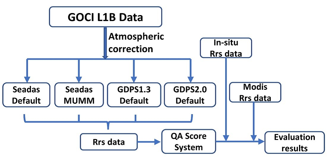
2.3. Algorithm
2.3.1. Atmospheric-Correction Algorithms of GDPS
2.3.2. Atmospheric-Correction Algorithms of SeaDAS
- (1)
- The aerosol multiple-scattering reflectance ratio of the two near-infrared bands of each pixel has a fixed value, defined as ε(745,865), then:where includes both Rayleigh and aerosol scatterings, as well as the interaction between them.
- (2)
- The ratio between reflectance and atmospheric transmission at the two near-infrared bands (α(745,865)) is constant and equal to 1.945.where is the water-leaving reflectance, and is the diffuse transmittance from the sun to the ocean atmosphere.
2.3.3. QA Score System
3. Results
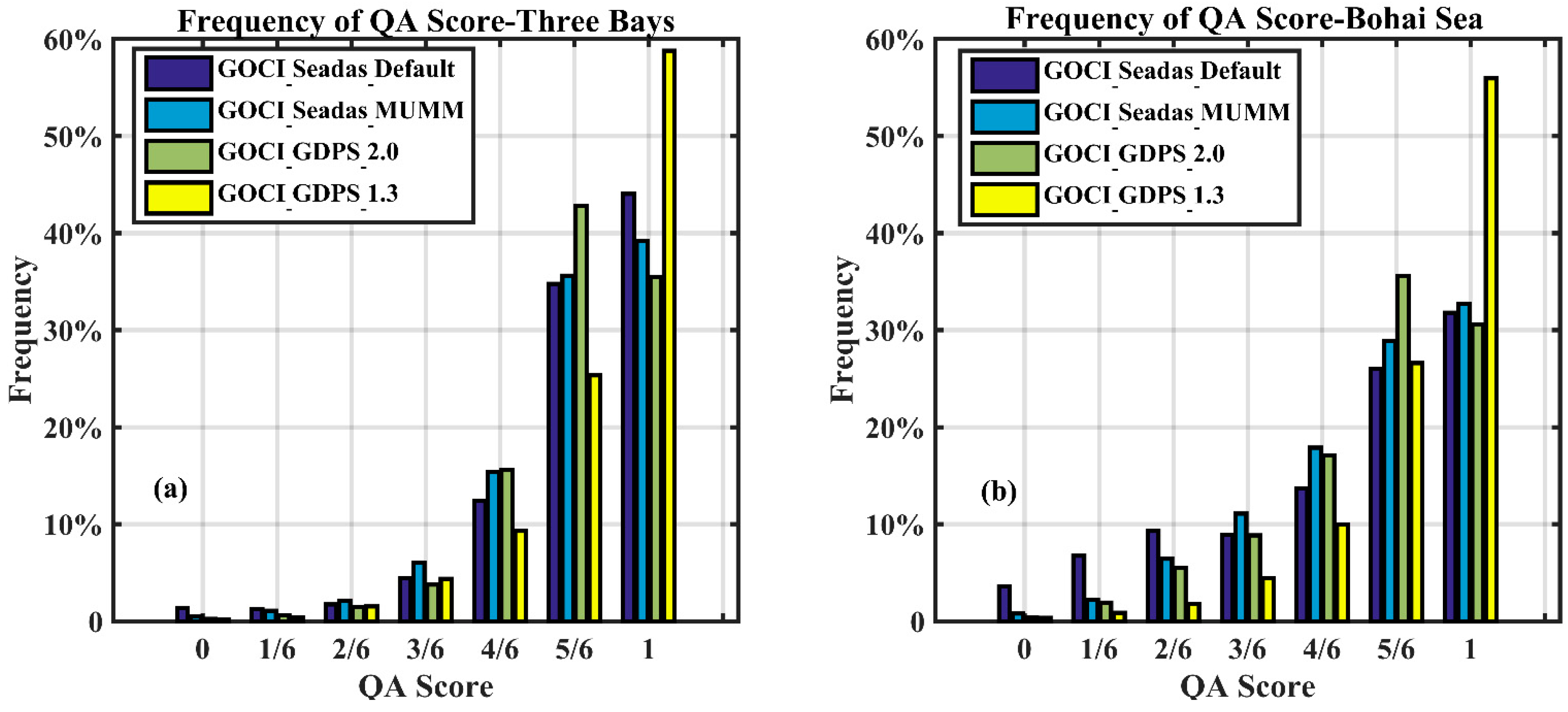
3.1. Statistical Analysis of the Rrs(λ) QA Score
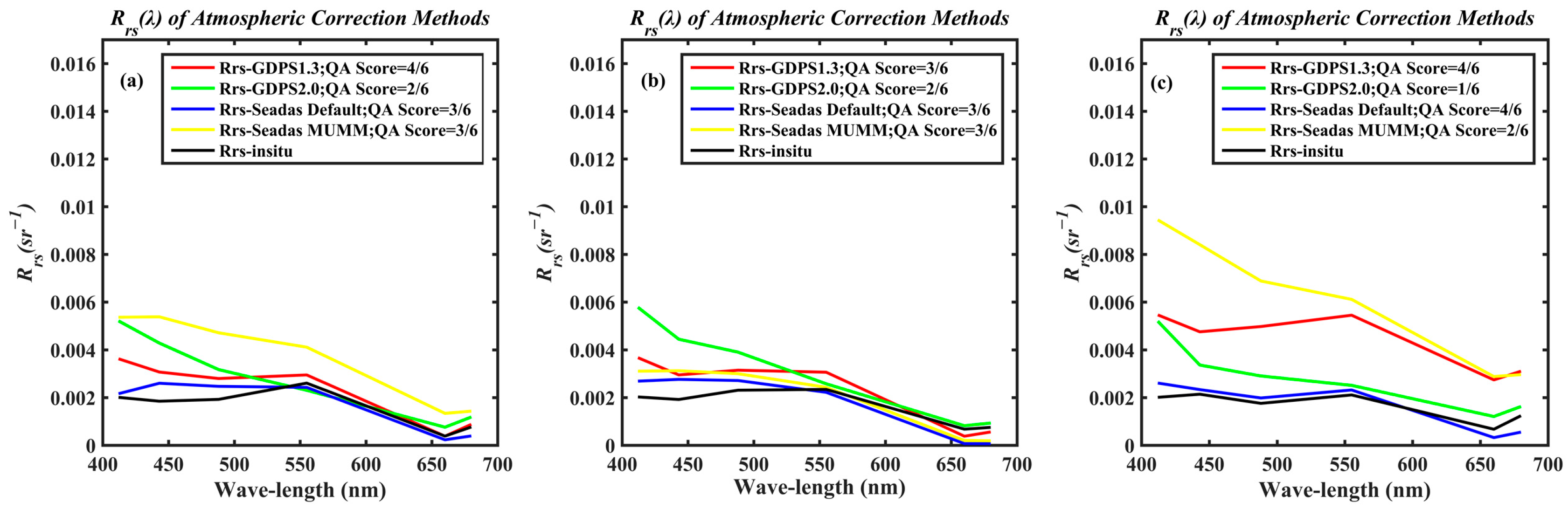
3.2. Comparison of Rrs(λ) with Measured In Situ Data
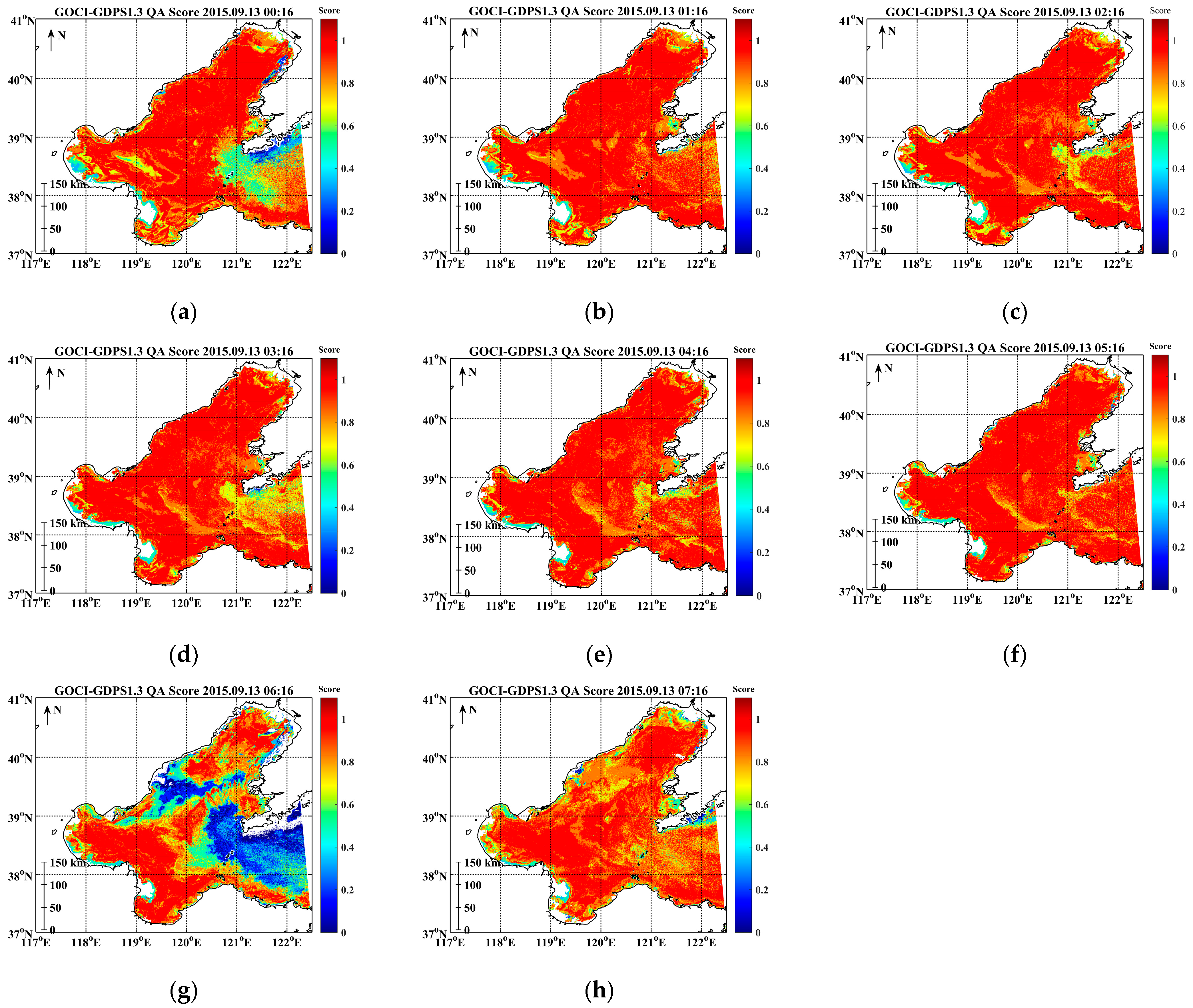
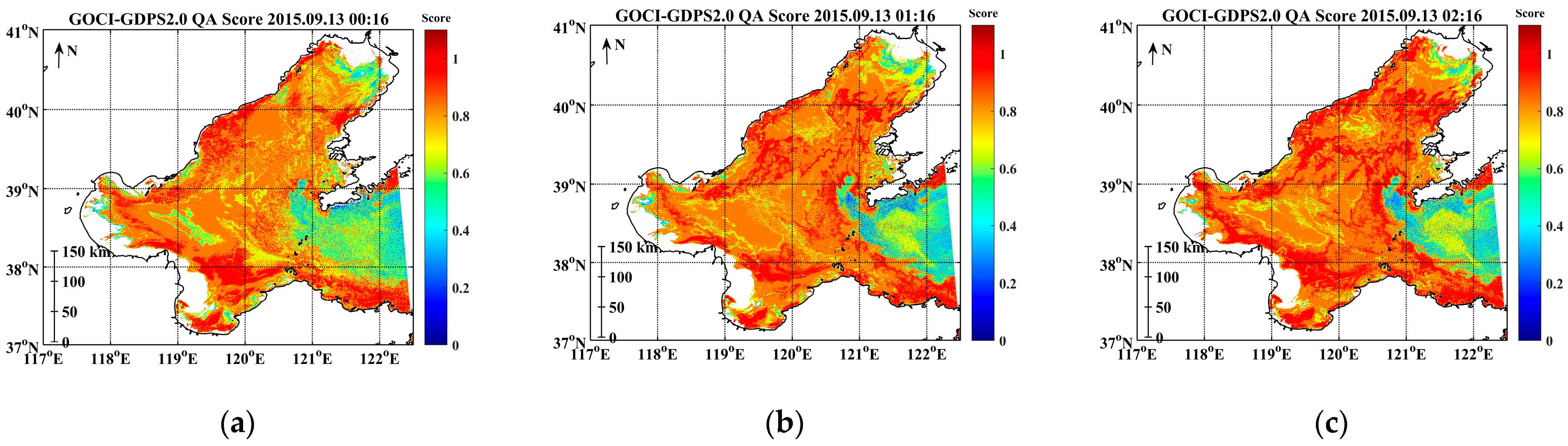
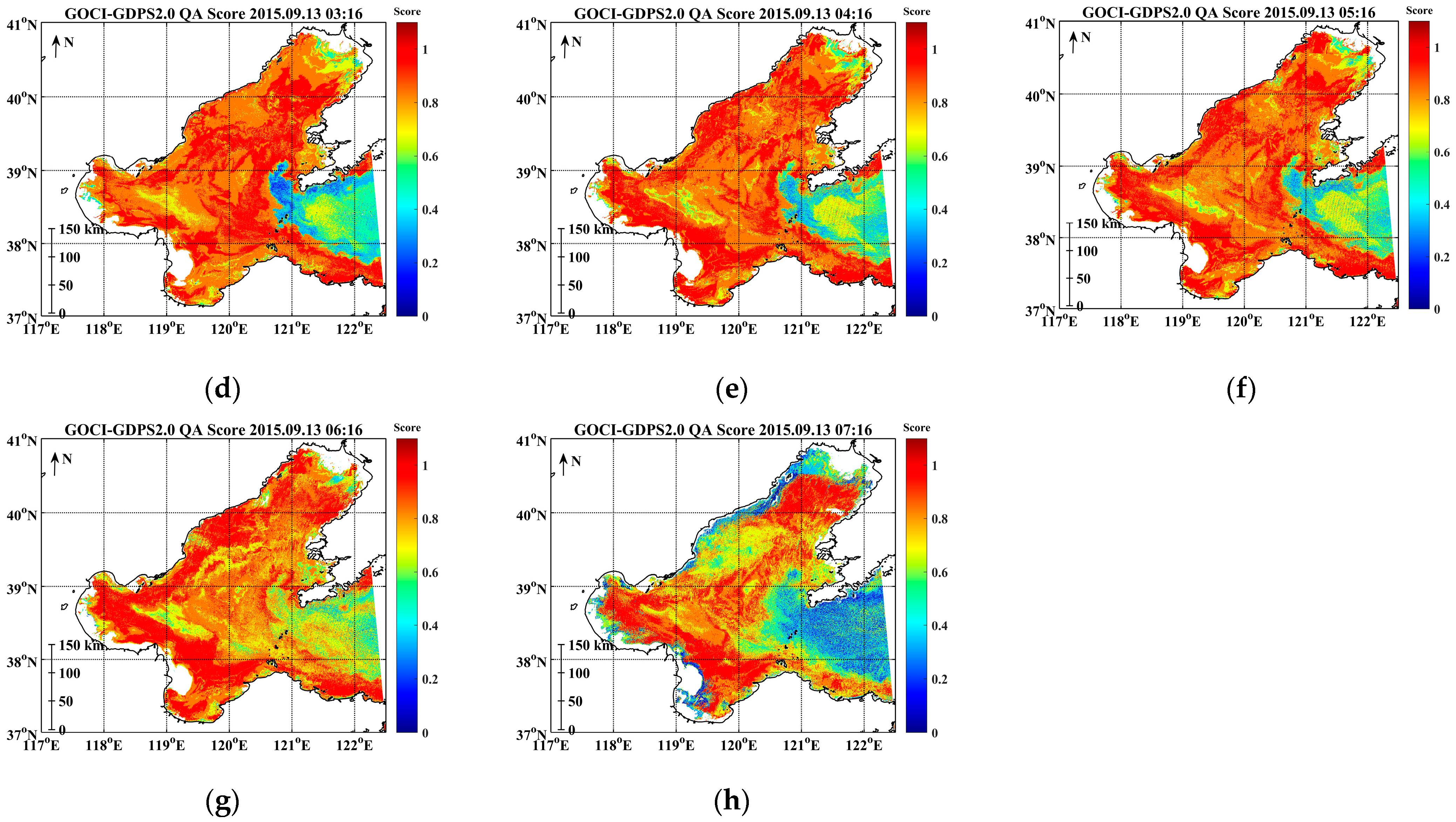
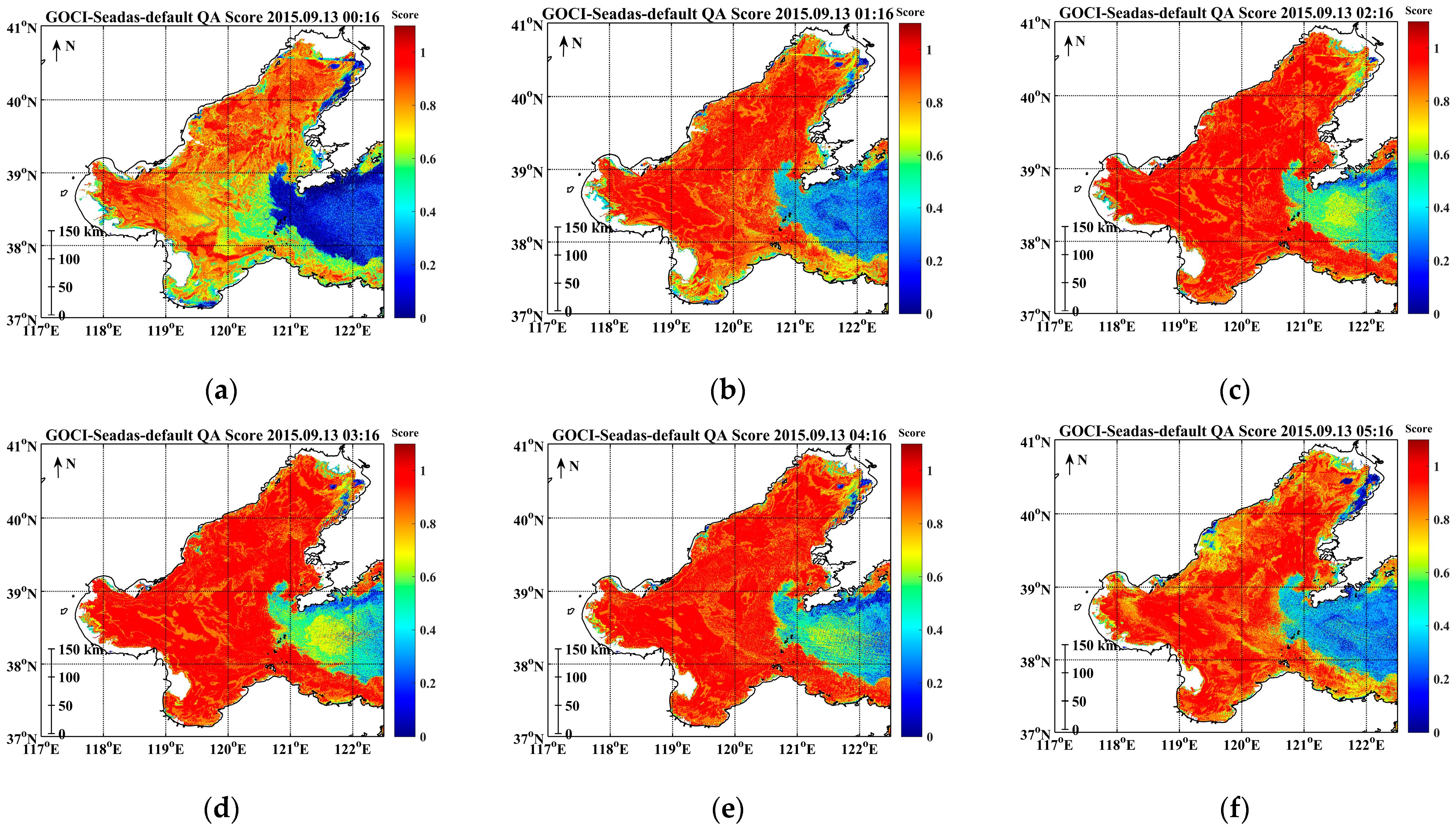
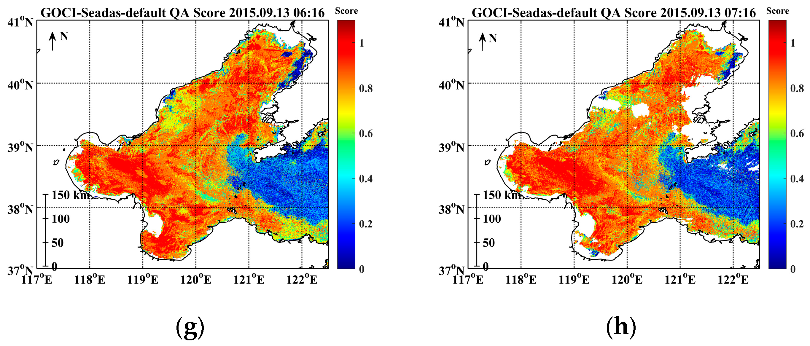
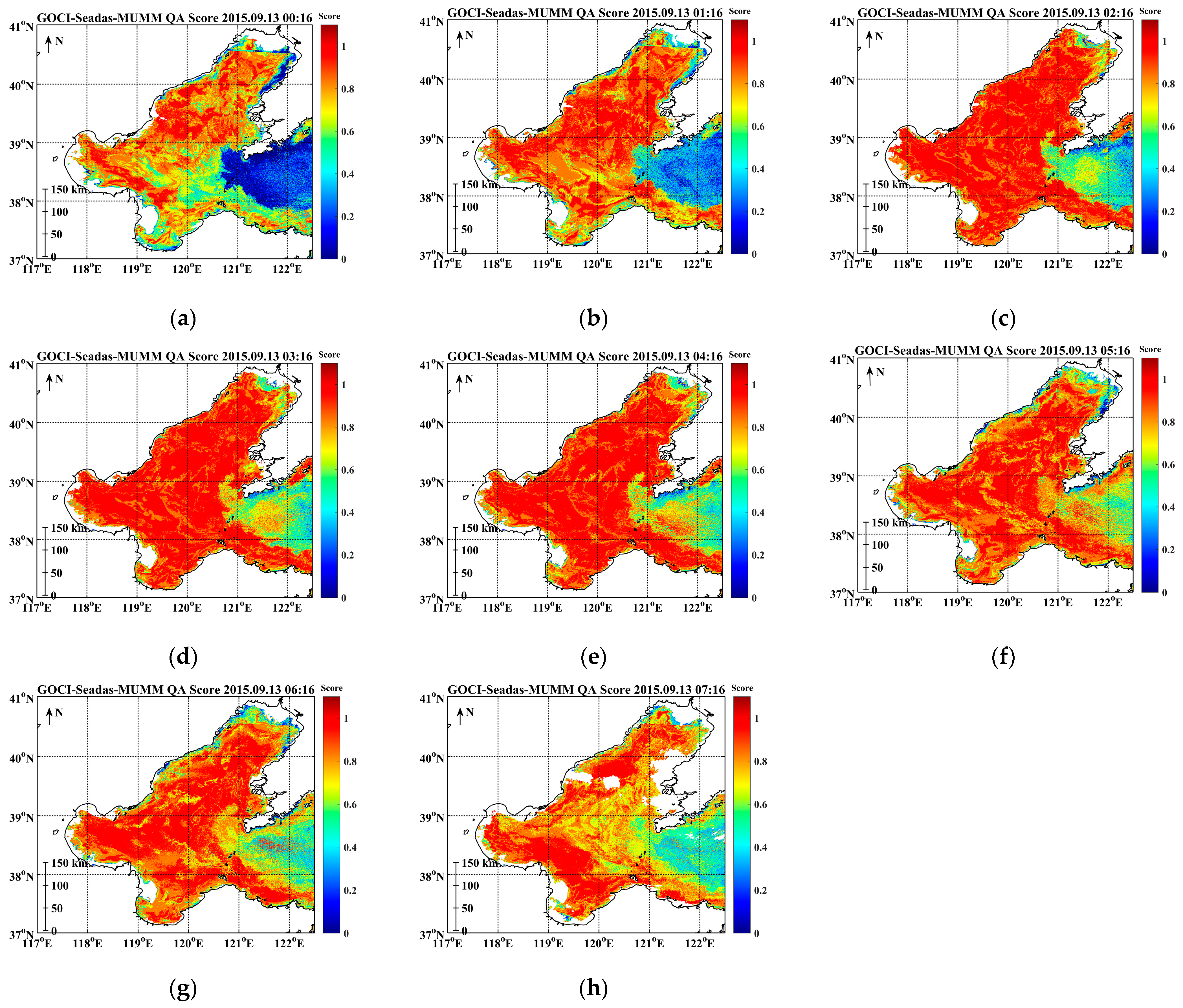
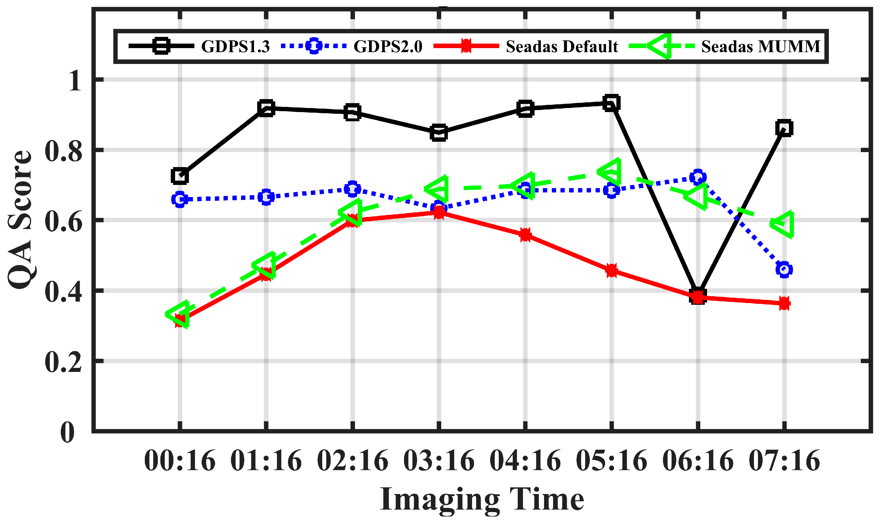
3.3. Hourly Variation of the GOCI Rrs(λ) QA Score from UTC 00:16 to 07:16
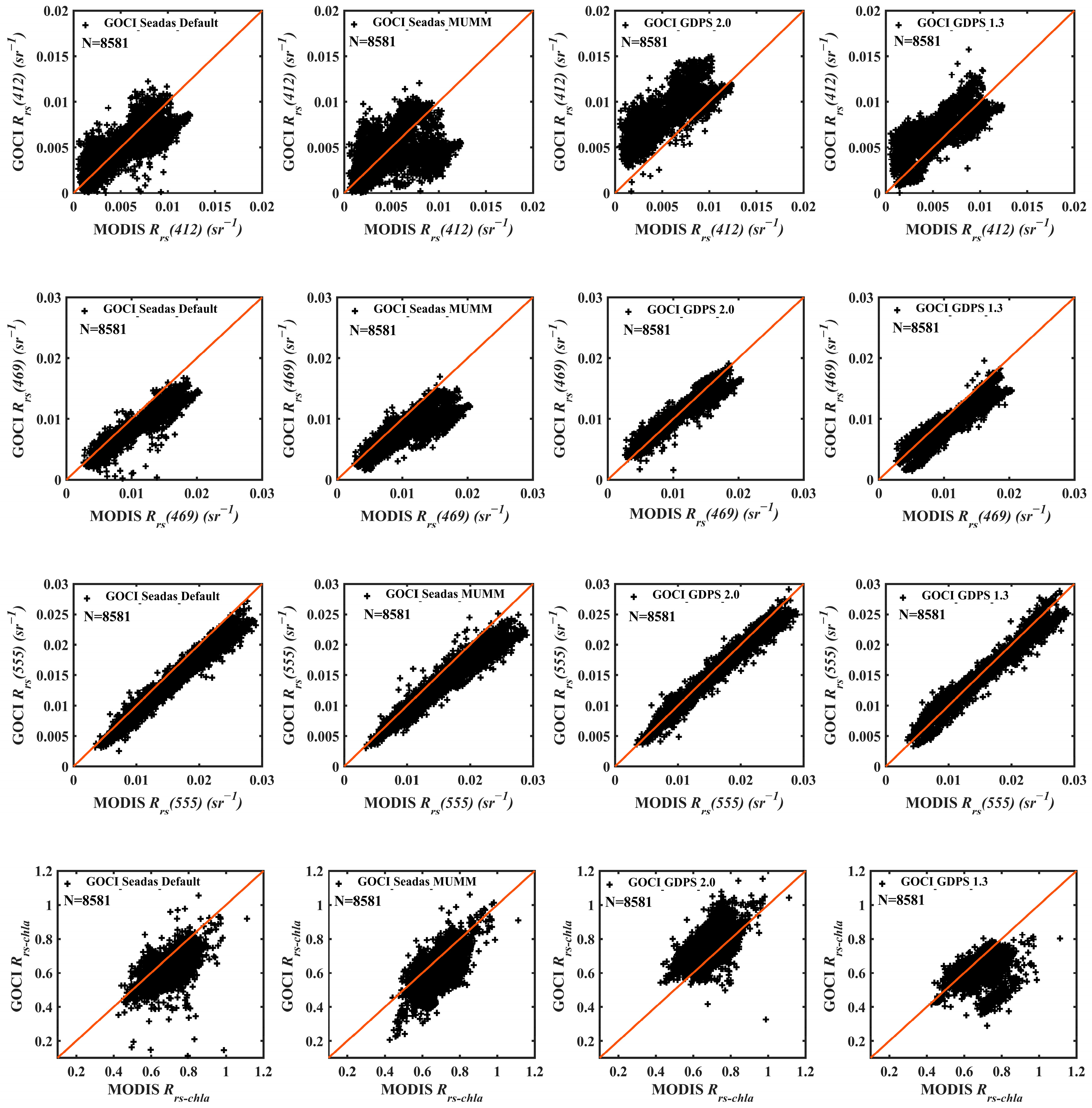
3.4. Cross-Comparison between GOCI and MODIS Rrs Data
4. Discussion
5. Conclusions
Author Contributions
Funding
Data Availability Statement
Acknowledgments
Conflicts of Interest
References
- Lee, Z.; Carder, K.L.; Arnone, R.A. Deriving inherent optical properties from water color: A multi-band quasi-analytical algorithm for optically deep waters. Appl. Opt. 2002, 41, 5755–5772. [Google Scholar] [CrossRef] [PubMed]
- Morel, A.; Prieur, L. Analysis of variations in ocean color. Limnol. Oceanogr. 1977, 22, 709–722. [Google Scholar] [CrossRef]
- Ryu, J.-H.; Han, H.-J.; Cho, S.; Park, Y.-J.; Ahn, Y.-H. Overview of geostationary ocean color imager (GOCI) and GOCI data processing system (GDPS). Ocean Sci. J. 2012, 47, 223–233. [Google Scholar] [CrossRef]
- Kim, D.-W.; Park, Y.-J.; Jeong, J.-Y.; Jo, Y.-H. Estimation of Hourly Sea Surface Salinity in the East China Sea Using Geostationary Ocean Color Imager Measurements. Remote Sens. 2020, 12, 755. [Google Scholar] [CrossRef] [Green Version]
- Cao, H.; Han, L. Hourly remote sensing monitoring of harmful algal blooms (HABs) in Taihu Lake based on GOCI images. Environ. Sci. Pollut. Res. 2021, 28, 35958–35970. [Google Scholar] [CrossRef]
- Kim, W.; Moon, J.-E.; Park, Y.-J.; Ishizaka, J. Evalution of chlorophyll retrievals from Geostationary Ocean color Imager (GOCI) for the North-East Asian region. Remote Sens. Environ. 2016, 184, 482–495. [Google Scholar] [CrossRef]
- Ling, Z.; Sun, D.; Wang, S.; Qiu, Z.; Huan, Y.; Mao, Z.; He, Y. Remote sensing estimation of colored dissolved organic matter (CDOM) from GOCI measurements in the Bohai Sea and Yellow Sea. Environ. Sci. Pollut. Res. 2020, 27, 6872–6885. [Google Scholar] [CrossRef]
- Bai, S.; Gao, J.; Sun, D.; Tian, M. Monitoring Water Transparency in Shallow and Eutrophic Lake Waters Based on GOCI Observations. Remote Sens. 2020, 12, 163. [Google Scholar] [CrossRef] [Green Version]
- Hsu, P.-C.; Lu, C.-Y.; Hsu, T.-W.; Ho, C.-R. Diurnal to Seasonal Variations in Ocean Chlorophyll and Ocean Currents in the North of Taiwan Observed by Geostationary Ocean Color Imager and Coastal Radar. Remote Sens. 2020, 12, 2853. [Google Scholar] [CrossRef]
- Minghelli, A.; Lei, M.; Charmasson, S.; Rey, V.; Chami, M. Monitoring Suspended Particle Matter Using GOCI Satellite Data after the Tohoku (Japan) Tsunami in 2011. IEEE J. Sel. Top. Appl. Earth Obs. Remote Sens. 2019, 12, 567–576. [Google Scholar] [CrossRef]
- Mao, Y.; Wang, S.; Qiu, Z.; Sun, D.; Bilal, M. Variations of transparency derived from GOCI in the Bohai Sea and the Yellow Sea. Opt. Express 2018, 26, 12191–12209. [Google Scholar] [CrossRef] [PubMed]
- Gordon, H.R. Removal of atmospheric effects from satellite imagery of the oceans. Appl. Opt. 1978, 17, 1631–1636. [Google Scholar] [CrossRef] [PubMed]
- Gordon, H.R.; Wang, M. Retrieval of water leaving radiance and aerosol optical thickness over the oceans with SeaWiFS: A preliminary algorithm. Appl. Opt. 1994, 33, 443–452. [Google Scholar] [CrossRef] [PubMed]
- Siegel, D.A.; Wang, M.; Maritorena, S.; Robinson, W. Atmospheric correction of satellite ocean color imagery: The black pixel assumption. Appl. Opt. 2000, 39, 3582–3591. [Google Scholar] [CrossRef]
- Wang, M.; Knobelspiesse, K.D.; McClain, C.R. Study of the Sea-Viewing Wide Field-of-View Sensor (SeaWiFS) aerosol optical property data over ocean in combination with the ocean color products. J. Geophys. Res. 2005, 110, 1–14. [Google Scholar] [CrossRef] [Green Version]
- Jamet, C.; Loisel, H.; Kuchinke, C.P. Comparison of three SeaWiFS atmospheric correction algorithms for turbid waters using AERONET-OC measurements. Remote Sens. Environ. 2011, 115, 1955–1965. [Google Scholar] [CrossRef]
- Goyens, C.; Jamet, C.; Schroeder, T. Evaluation of four atmospheric correction algorithms for MODIS-Aqua images over contrasted coastal waters. Remote Sens. Environ. 2013, 131, 63–75. [Google Scholar] [CrossRef]
- Ahn, J.-H.; Park, Y.-J. Estimating Water Reflectance at Near-Infrared Wavelengths for Turbid Water Atmospheric Correction: A Preliminary Study for GOCI-II. Remote Sens. 2020, 12, 3791. [Google Scholar] [CrossRef]
- Wang, M.; Shi, W. The NIR-SWIR combined atmospheric correction approach for MODIS ocean color data processing. Opt. Express 2007, 15, 15722–15733. [Google Scholar] [CrossRef] [Green Version]
- Wang, M.; Shi, W. Remote Sensing of the Ocean Contributions from Ultraviolet to Near-Infrared Using the ShortwaveInfrared Bands: Simulations. Appl. Opt. 2007, 46, 1535–1547. [Google Scholar] [CrossRef]
- Oo, M.; Vargas, M.; Gilerson, A.; Gross, B.; Moshary, F.; Ahmed, S. Improving atmospheric correction for highly productive coastal waters using the short wave infrared retrieval algorithm with water-leaving reflectance constraints at 412 nm. Appl. Opt. 2008, 47, 3846–3859. [Google Scholar] [CrossRef] [PubMed]
- He, X.; Bai, Y.; Pan, D.; Junwu, T.; Difeng, W. Atmospheric correction of satellite ocean color imagery using the ultraviolet wavelength for highly turbid waters. Opt. Express 2012, 20, 20754–20770. [Google Scholar] [CrossRef] [PubMed]
- Hu, C.; Carder, K.L.; Muller-Karger, F.E. Atmospheric correction of SeaWiFS imagery over turbid coastal waters: A practical method. Remote Sens. Environ. 2000, 74, 195–206. [Google Scholar] [CrossRef]
- Ruddick, K.G.; Ovidio, F.; Rijkeboer, M. Atmospheric correction of SeaWiFS imagery for turbid coastal and inland waters. Appl. Opt. 2000, 39, 897–912. [Google Scholar] [CrossRef] [Green Version]
- Wang, M.; Shi, W.; Jiang, L. Atmospheric correction using near-infrared bands for satellite ocean color data processing in the turbid western Pacific region. Opt. Express 2012, 20, 741–753. [Google Scholar] [CrossRef]
- Ahn, J.-H.; Park, Y.-J.; Fukushima, H. Comparison of Aerosol Reflectance Correction Schemes Using Two Near-Infrared Wavelengths for Ocean Color Data Processing. Remote Sens. 2018, 10, 1791. [Google Scholar] [CrossRef] [Green Version]
- AHN, J.-H.; PARK, Y.-J.; KIM, W.; LEE, B. Simple aerosol correction technique based on the spectral relationships of the aerosol multiple-scattering reflectances for atmospheric correction over the oceans. Opt. Express 2016, 24, 29659–29669. [Google Scholar] [CrossRef]
- Stumpf, R.P.; Arnone, R.A.; Gould, R.W.; Martinolich, P.M.; Ransibrahmanakul, V. A Partially Coupled Ocean-Atmosphere Model for Retrieval of Water-Leaving Radiance from SeaWiFS in Coastal Waters. NASA Tech. Memo. 2003, 206892, 51–59. [Google Scholar]
- Lavender, S.J.; Pinkerton, M.H.; Moore, G.F.; Aiken, J.; Blondeau-Patissier, D. Modification to the atmospheric correction of SeaWiFS ocean colour images over turbid waters. Cont. Shelf Res. 2005, 25, 539–555. [Google Scholar] [CrossRef]
- Jamet, C.; Thiria, S.; Moulin, C. Use of a Neurovariational Inversion for Retrieving Oceanic and Atmospheric Constituents from Ocean Color Imagery: A Feasibility Study. J. Atmos. Ocean. Tech. 2005, 22, 460–475. [Google Scholar] [CrossRef]
- Schroeder, T.; Behnert, I.; Schaale, M.; Fischer, J.; Doerffer, R. Atmospheric correction algorithm for MERIS above case-2 waters. J. Remote Sens. 2007, 28, 1469–1486. [Google Scholar] [CrossRef]
- Brajard, J.; Santer, R.; Crpon, M.; Thiria, S. Atmospheric correction of MERIS data for case-2 waters using a neuro-variational inversion. Remote Sens. Environ. 2012, 126, 51–61. [Google Scholar] [CrossRef]
- Brajard, J.; Jamet, C.; Thiria, S.; Moulin, C.; Crepon, M. Use of a neuro-variational inversion for retrieving oceanic and atmospheric constituents from satellite ocean color sensor: Application to absorbing aerosols. Neural Netw. 2006, 22, 460–475. [Google Scholar] [CrossRef]
- Kuchinke, C.P.; Gordon, H.R.; Harding, L.W.; Voss, K.J. Spectral optimization for constituent retrieval in Case II waters II: Validation study in the Chesapeake Bay. Remote Sens. Environ. 2009, 113, 610–621. [Google Scholar] [CrossRef]
- Chomko, R.; Gordon, H.; Maritorena, S.; Siegel, D. Simultaneous retrieval of oceanic and atmospheric parameters for ocean color imagery by spectral optimization: A validation. Remote Sens. Environ. 2003, 84, 208–220. [Google Scholar] [CrossRef]
- Zibordi, G.; Berthon, J.-F.; Melin, F.; Alimonte, D.; Kaitala, S. Validation of satellite ocean color primary products at optically complex coastal sites: Northern Adriatic Sea, Northern Baltic Proper and Gulf of Finland. Remote Sens. Environ. 2009, 113, 2574–2591. [Google Scholar] [CrossRef]
- Huang, X.; Zhu, J.; Han, B.; Jamet, C.; Tian, Z.; Zhao, Y.; Li, J.; Li, T. Evaluation of Four Atmospheric Correction Algorithms for GOCI Images over the Yellow Sea. Remote Sens. 2019, 11, 1631. [Google Scholar] [CrossRef] [Green Version]
- Zhang, M.; Hu, C.; Cannizzaro, J.; English, D.; Barnes, B.B.; Carlson, P.; Yarbro, L. Comparison of two atmospheric correction approaches applied to MODIS measurements over North American waters. Remote Sens. Environ. 2018, 216, 442–455. [Google Scholar] [CrossRef]
- Bailey, S.W.; Werdell, P.J. A multi-sensor approach for the on-orbit validation of ocean color satellite data products. Remote Sens. Environ. 2006, 102, 12–23. [Google Scholar] [CrossRef]
- Salama, M.S.; Stein, A. Error decomposition and estimation of inherent optical properties. Appl. Opt. 2009, 48, 4947–4962. [Google Scholar] [CrossRef] [PubMed]
- Wang, M.; Son, S. VIIRS-derived chlorophyll-a using the ocean color index method. Remote Sens. Environ. 2016, 182, 141–149. [Google Scholar] [CrossRef]
- Guo, S.; Sun, B.; Zhang, H.K.; Liu, J.; Chen, J.; Wang, J.; Jiang, X.; Yang, Y. MODIS ocean color product downscaling via spatio-temporal fusion and regression: The case of chlorophyll-a in coastal waters. Int. J. Appl. Earth Obs. Geoinf. 2018, 73, 340–361. [Google Scholar] [CrossRef]
- Wei, J.; Lee, Z.; Shang, S. A system to measure the data quality of spectral remote sensing reflectance of aquatic environments. J. Geophys. Res. Ocean. 2016, 121, 8189–8207. [Google Scholar] [CrossRef]
- Ahn, J.H.; Park, Y.J.; Kim, W.; Lee, B. Vicarious calibration of the geostationary ocean color imager. Opt. Express 2015, 23, 23236–23258. [Google Scholar] [CrossRef]
- Ahn, J.-H.; Park, Y.-J.; Ryu, J.-H.; Lee, B.; Oh, I.S. Development of atmospheric correction algorithm for Geostationary Ocean Color Imager (GOCI). Ocean. Sci. J. 2012, 47, 247–259. [Google Scholar] [CrossRef]
- He, M.; He, S.; Zhang, X.; Zhou, F.; Li, P. Assessment of Normalized Water-Leaving Radiance Derived from GOCI Using AERONET-OC Data. Remote Sens. 2021, 13, 1640. [Google Scholar] [CrossRef]
- Chavula, G.; Brezonik, P.; Thenkabail, P.; Johnson, T.; Bauer, M. Estimating chlorophyll concentration in Lake Malawi from MODIS satellite imagery. Phys. Chem. Earth Parts A/B/C 2009, 34, 755–760. [Google Scholar] [CrossRef]
- NASA SeaDAS. Available online: https://seadas.gsfc.nasa.gov/history/ (accessed on 15 June 2021).
- Shang, S.; Lee, Z.; Shi, L.; Lin, G.; Wei, G.; Li, X. Changes in water clarity of the Bohai Sea: Observations from MODIS. Remote Sens. Environ. 2016, 186, 22–31. [Google Scholar] [CrossRef] [Green Version]
- Bailey, S.W.; Franz, B.A.; Werdell, P.J. Estimation of near-infraredwater-leaving reflectance for satellite ocean color data processing. Opt. Express 2010, 18, 7521–7527. [Google Scholar] [CrossRef]
- Kruse, F.A.; Lefkoff, A.B.; Boardman, J.B.; Heidebrecht, K.B.; Shapiro, A.T.; Barloon, P.J.; Goetz, A.F.H. The spectral image processing system (SIPS)—Interactive visualization and analysis of imaging spectrometer data. Remote Sens. Environ. 1993, 44, 145–163. [Google Scholar] [CrossRef]


| Band | MODIS Wavelength (nm) | Band | GOCI Wavelength (nm) |
|---|---|---|---|
| 1 | 412 | 1 | 412 |
| 2 | 443 | 2 | 443 |
| 3 | 469 | 3 | 490 |
| 4 | 488 | 4 | 555 |
| 5 | 531 | 5 | 660 |
| 6 | 547 | 6 | 680 |
| 7 | 555 | 7 | 745 |
| 8 | 667 | 8 | 865 |
| 9 | 678 | ||
| 10 | 748 | ||
| 11 | 859 | ||
| 12 | 869 |
| λ1 (nm) | 555 | 555 | 555 | 745 | 745 | 745 | 865 |
| λ2 (nm) | 412 | 430 | 490 | 555 | 660 | 680 | 745 |
| D | 4 | 4 | 4 | 4 | 3 | 3 | 2 |
| QA Score | Frequency | |||
|---|---|---|---|---|
| Seadas—Default | Seadas—MUMM | GDPS2.0 | GDPS1.3 | |
| 0 | 2.48% | 0.65% | 0.34% | 0.29% |
| 1/6 | 3.98% | 1.67% | 1.28% | 0.66% |
| 2/6 | 5.51% | 4.28% | 3.50% | 1.68% |
| 3/6 | 6.68% | 8.56% | 6.32% | 4.42% |
| 4/6 | 13.05% | 16.65% | 16.36% | 9.63% |
| 5/6 | 30.39% | 32.24% | 39.17% | 25.96% |
| 1 | 37.91% | 35.96% | 33.05% | 57.36% |
| Area | QA Score | Frequency | |||
|---|---|---|---|---|---|
| Seadas—Default | Seadas—MUMM | GDPS2.0 | GDPS1.3 | ||
| Three Bays | 0 | 1.36% | 0.488% | 0.241% | 0.22% |
| 1/6 | 1.24% | 1.100% | 0.621% | 0.44% | |
| 2/6 | 1.74% | 2.155% | 1.474% | 1.54% | |
| 3/6 | 4.45% | 6.034% | 3.784% | 4.39% | |
| 4/6 | 12.41% | 15.407% | 15.612% | 9.30% | |
| 5/6 | 34.78% | 35.613% | 42.780% | 25.33% | |
| 1 | 44.02% | 39.203% | 35.487% | 58.78% | |
| Bohai Sea | 0 | 3.60% | 0.81% | 0.43% | 0.35% |
| 1/6 | 6.73% | 2.23% | 1.94% | 0.87% | |
| 2/6 | 9.28% | 6.41% | 5.52% | 1.82% | |
| 3/6 | 8.91% | 11.08% | 8.85% | 4.46% | |
| 4/6 | 13.69% | 17.89% | 17.10% | 9.96% | |
| 5/6 | 26.00% | 28.86% | 35.56% | 26.60% | |
| 1 | 31.79% | 32.72% | 30.60% | 55.95% | |
| Rrs | Atmospheric Correction Algorithms | ε | RMSE | Mean of QA Score |
|---|---|---|---|---|
| Rrs(469) | Seadas—Default | 30.31% | 0.00091 | 0.595 |
| Seadas—MUMM | 76.59% | 0.00309 | 0.476 | |
| GDPS2.0 | 54.59% | 0.00172 | 0.310 | |
| GDPS1.3 | 59.26% | 0.00198 | 0.643 | |
| Rrs(555) | Seadas—Default | 11.13% | 0.00031 | 0.595 |
| Seadas—MUMM | 50.26% | 0.00212 | 0.476 | |
| GDPS2.0 | 15.84% | 0.00048 | 0.310 | |
| GDPS1.3 | 51.01% | 0.00192 | 0.643 | |
| Rrs(469)/Rrs(555) | Seadas—Default | 22.96% | 0.26533 | 0.595 |
| Seadas—MUMM | 29.82% | 0.32298 | 0.476 | |
| GDPS2.0 | 43.04% | 0.50643 | 0.310 | |
| GDPS1.3 | 10.34% | 0.10863 | 0.643 |
| Band (nm) | Atmospheric Correction Algorithms | r | ε | RMSE | QA Score |
|---|---|---|---|---|---|
| 412 | Seadas—Default | 0.832 | 27.53% | 0.00133 | 0.938 |
| Seadas—MUMM | 0.580 | 38.72% | 0.00199 | 0.922 | |
| GDPS2.0 | 0.847 | 73.07% | 0.00364 | 0.921 | |
| GDPS1.3 | 0.800 | 56.70% | 0.00247 | 0.967 | |
| 443 | Seadas—Default | 0.932 | 15.96% | 0.00129 | 0.938 |
| Seadas—MUMM | 0.817 | 19.14% | 0.00186 | 0.922 | |
| GDPS2.0 | 0.939 | 26.39% | 0.00181 | 0.921 | |
| GDPS1.3 | 0.904 | 19.61% | 0.00136 | 0.967 | |
| 490 | Seadas—Default | 0.971 | 20.78% | 0.00201 | 0.938 |
| Seadas—MUMM | 0.939 | 19.70% | 0.00230 | 0.922 | |
| GDPS2.0 | 0.978 | 7.12% | 0.00087 | 0.921 | |
| GDPS1.3 | 0.962 | 9.38% | 0.00126 | 0.967 | |
| 531 | Seadas—Default | 0.985 | 16.24% | 0.00197 | 0.938 |
| Seadas—MUMM | 0.974 | 15.46% | 0.00220 | 0.922 | |
| GDPS2.0 | 0.986 | 5.29% | 0.00091 | 0.921 | |
| GDPS1.3 | 0.980 | 7.24% | 0.00113 | 0.967 | |
| 555 | Seadas—Default | 0.988 | 13.91% | 0.00180 | 0.938 |
| Seadas—MUMM | 0.979 | 13.32% | 0.00204 | 0.922 | |
| GDPS2.0 | 0.989 | 5.65% | 0.00096 | 0.921 | |
| GDPS1.3 | 0.982 | 7.68% | 0.00112 | 0.967 | |
| 660 | Seadas—Default | 0.982 | 30.57% | 0.00129 | 0.938 |
| Seadas—MUMM | 0.967 | 29.01% | 0.00158 | 0.922 | |
| GDPS2.0 | 0.983 | 10.04% | 0.00063 | 0.921 | |
| GDPS1.3 | 0.977 | 24.88% | 0.00105 | 0.967 |
| Rrs | Atmospheric Correction Algorithms | ε | RMSE | QA Score |
|---|---|---|---|---|
| Rrs(469) | Seadas—Default | 23.91% | 0.00212 | 0.938 |
| Seadas—MUMM | 22.62% | 0.00248 | 0.922 | |
| GDPS2.0 | 9.42% | 0.00102 | 0.921 | |
| GDPS1.3 | 11.98% | 0.00153 | 0.967 | |
| Rrs(555) | Seadas—Default | 13.91% | 0.00180 | 0.938 |
| Seadas—MUMM | 13.32% | 0.00204 | 0.922 | |
| GDPS2.0 | 5.65% | 0.00096 | 0.921 | |
| GDPS1.3 | 7.68% | 0.00112 | 0.967 | |
| Rrs-chla | Seadas—Default | 10.65% | 0.08833 | 0.938 |
| Seadas—MUMM | 10.79% | 0.08751 | 0.922 | |
| GDPS2.0 | 10.81% | 0.09669 | 0.921 | |
| GDPS1.3 | 9.70% | 0.08674 | 0.967 |
Publisher’s Note: MDPI stays neutral with regard to jurisdictional claims in published maps and institutional affiliations. |
© 2022 by the authors. Licensee MDPI, Basel, Switzerland. This article is an open access article distributed under the terms and conditions of the Creative Commons Attribution (CC BY) license (https://creativecommons.org/licenses/by/4.0/).
Share and Cite
Liu, X.; Yang, Q.; Wang, Y.; Zhang, Y. Evaluation of GOCI Remote Sensing Reflectance Spectral Quality Based on a Quality Assurance Score System in the Bohai Sea. Remote Sens. 2022, 14, 1075. https://doi.org/10.3390/rs14051075
Liu X, Yang Q, Wang Y, Zhang Y. Evaluation of GOCI Remote Sensing Reflectance Spectral Quality Based on a Quality Assurance Score System in the Bohai Sea. Remote Sensing. 2022; 14(5):1075. https://doi.org/10.3390/rs14051075
Chicago/Turabian StyleLiu, Xiaoyan, Qian Yang, Yunhua Wang, and Yu Zhang. 2022. "Evaluation of GOCI Remote Sensing Reflectance Spectral Quality Based on a Quality Assurance Score System in the Bohai Sea" Remote Sensing 14, no. 5: 1075. https://doi.org/10.3390/rs14051075