Article

A Methodology to Generate Integrated Land Cover Data for Land Surface Model by Improving Dempster-Shafer Theory

School of Geographical Sciences, Nanjing University of Information Science and Technology, Nanjing 210044, China
*
Author to whom correspondence should be addressed.
Remote Sens. 2022, 14(4), 972; https://doi.org/10.3390/rs14040972
Submission received: 14 January 2022 / Revised: 12 February 2022 / Accepted: 13 February 2022 / Published: 16 February 2022
(This article belongs to the Special Issue Remote Sensing for Mapping Global Land Surface Parameters)

Abstract

:
Land cover type is a key parameter for simulating surface processes in many land surface models (LSMs). Currently, the widely used global remote sensing land cover products cannot meet the requirements of LSMs for classification systems, physical definition, data accuracy, and space-time resolution. Here, a new fusion method was proposed to generate land cover data for LSMs by fusing multi-source remote sensing land cover data, which was based on improving Dempster-Shafer evidence theory with mathematical models and knowledge rules optimization. The new method has the ability to deal with seriously disagreement information, thereby improving the robustness of the theory. The results showed the new method can reduce the disagreement between input data and realized the conversion of multiple land cover classification systems to into a single land cover classification system. China Fusion Land Cover data (CFLC) in 2015 generated by the new method maintained the classification accuracy of the China land use map (CNLULC), which is based on visual image interpretation and further enriched land cover classes of input data. Compared with Geo-Wiki observations in 2015, the overall accuracy for CFLC is higher than other two global land cover data. Compared with the observations, the 0–10 cm soil moisture simulated by the CFLC in Noah–MP LSM during the growing season in 2014 had better performance than that simulated by initial land cover data and MODIS land cover data. Our new method is highly portable and generalizable to generate higher quality land cover data with a specific land cover classification system for LSMs by fusing multiple land cover data, providing a new approach to land cover mapping for LSMs.

Graphical Abstract

1. Introduction

Land cover type is a key parameter for many land surface models (LSMs), such as the simple biosphere model (SiB) [1], common land model (CLM) [2], and the community Noah land surface model with multi-parameterization options (Noah-MP) [3], which is widely used to simulate the water and energy processes and material exchange between the land and atmosphere. Some key parameters of the underlying surface, such as surface roughness and albedo, can be directly determined from the parameter table in LSMs based on land cover types [4,5]. Therefore, high-quality land cover data can provide accurate underlying surface information for LSMs to improve the model simulation, which is one of the important basic data for understanding and simulating the surface process accurately [6].
Currently, remote sensing technologies have become an important means of obtaining land cover information at global and regional scales. Multiple global or regional land cover data are available for download, such as the UMD land cover data established by the University of Maryland (UMD) [7], moderate-resolution imaging spectroradiometer land cover data (MODIS LC) established by the National Aeronautics and Space Administration (NASA) [8], and GlobCover established by the European Space Agency (ESA) [9]. One of the major problems of these remote sensing land cover products is the lack of interoperability among them, since their development was driven by different initiatives with different objectives. Considering that these land cover products are often not specifically designed and produced for LSMs, it is difficult for a single land cover dataset to meet the usage requirements of LSMs in classification systems, category definition, and space-time resolution of land features, severely restricting the development and application of LSMs in climate change, disaster monitoring, and ecosystem management [10,11,12].
A remedy to this is the integration of various sources of land cover data into a single framework for LSMs using multi-source data fusion approaches [13]. Multi-source data fusion methods refer to the automatic or semi-automatic conversion of data from different sources and different time points into the same form through a certain mathematical algorithm [14]. The fusion methods compensate for the deficiencies of a single datum by complementing with another data source in terms of spatio-temporal resolution, spatial consistency, and data accuracy. Multi-source remote sensing data fusion can be classified into three different categories, including the pixel level, the feature level, and the decision level [15]. Pixel-level fusion and feature-level fusion are widely used in the fusion of multiple remote sensing spectral data, which are difficult to be applied to the fusion of remote sensing land cover data [16]. Since each pixel of remote sensing land cover data has a specific physical meaning, the fusion of these data often adopts decision-level fusion, i.e., combining the remote sensing land cover data from multiple algorithms to yield a final fused decision. Currently, various decision level fusion methods have been developed, mainly including the data consistency method, fuzzy set theory, and geographic statistical methods [17,18,19]. Data consistency methods analyze the consistency of multiple remote sensing data and establish fusion rules to realize the fusion of multi-source remote sensing data. However, data consistency methods need to score the input data to determine the priority of different input data in the fusion process. Scoring disasters are prone to occur, owing to the diversity and complexity of evaluation indicators [20]. The fuzzy set methods flexibilize attribution in the ordinary set, expanding the ordinary feature set (0, 1) to the closed interval (0, 1), and use the feature function to calculate the fuzzy attribution degree, which can maximize the preservation of the local credibility of different remote sensing products during the fusion process. However, the methods based on fuzzy set theory seldom consider the setting of pixel weights and product weights in the fusion process, leading to a lack of credibility in the fusion results [21]. Geographic statistical methods, such as geographically weighted regression (GWR) and spatial logistic regression (SLR), establish the statistical relationship between the measured sample points and various remote sensing data to predict data in the area without sample points so as to obtain the fusion result. However, methods based on geographic statistic are limited by the lack of scalability of a single statistic model, which makes it difficult to apply to different regions [22]. In addition, statistical analysis of multiple regions tends to increase the cost and difficulty of the research. Overall, classic decision-level fusion methods are difficult to be directly applied to the integration of land cover data for LSM.
Many studies have been devoted to applying classic decision-level fusion methods to generate integrated land cover data, which showed that the fusion of multi-source land cover data could improve data accuracy [13,16,23]. However, these classic decision-level fusion methods, such as the data consistency method and fuzzy set method, are highly subjective and have greater uncertainty when dealing with the fusion of multiple conflicting data. In recent years, advanced artificial intelligence methods have been introduced into the fusion of multi-source land cover data [24,25]. Artificial intelligence methods, such as random forest and deep learning, have the ability to deal with non-linear problems in the fusion process [26]. Considering that the land cover types of each pixel have complex physical definitions, current artificial intelligence methods lack strong interpretability in dealing with these physical definitions, failing to ensure the accuracy of land cover fusion [27]. Therefore, combining artificial intelligence methods with human knowledge rules can significantly improve the strong subjectivity and the weak ability to deal with nonlinear problems of traditional land cover fusion methods; however, related research is still limited.
In this study, we aimed to develop a new fusion method to generate land cover data for LSMs. Our new method reduced the disagreement between input data and realized the conversion of multiple land cover classification systems to an LSM classification system by improving Dempster-Shafer (D-S) evidence theory, which belongs to the category of artificial intelligence with mathematical models and knowledge rules optimization. Furthermore, we evaluated the reliability of our new method, including site-based verification, cross-comparison between multiple products, and the effect of the new integrated land cover data on Noah-MP LSM for 0–10 cm soil moisture simulation over China.

2. Materials and Methods

2.1. Land Cover Data

Consider the time consistency of all fusion data and time requirements for further LSM simulations, China land use data (CNLULC), MODIS LC and fine resolution observation and monitoring of global land cover (FROM-GLC) in 2015 were used as input data in this study, while the China vegetation map was collected as auxiliary data for the fusion. Currently, the China National Meteorological Information Center is developing a new generation of high resolution land data assimilation system (HRCLDAS-V1.0), which will reach a spatial resolution of 0.01° (1 km) [28]. In order to be able to interface with the HRCLDAS-V1.0 system in the future, we used 0.01° as the fusion spatial resolution. The spatial resolutions of MODIS LC, FROM-GLC, and CNLULC are 500 m, 30 m, and 1 km, respectively. MODIS LC and FROM-GLC were up-scaled to convert their spatial resolution to 0.01° by the method of majority sampling of pixels, i.e., we took the pixel type with the largest proportion in the 0.01° grid as the pixel type after resampling.

2.1.1. CNLULC

The CNLULC data are based on the visual image interpretation of Landsat images by experts from all over the country [29]. The data are updated every five years, and the national scale data have so far been updated to 2018. They are currently the most accurate remote sensing land cover data in China, with classification accuracy of more than 95%. However, their classification system lacks descriptions of vegetation type and seasonal characteristics, which are difficult to be applied in land surface simulations [30]. In this study, CNLULC at 1 km spatial resolution in 2015 was used as input data, which were obtained from the Resource and Environmental Science Data Center of the Chinese Academy of Sciences.

2.1.2. MODIS LC

The MODIS LC is a product of the environmental remote sensing satellites Terra and Aqua launched by NASA. It is obtained by supervising the classification of MODIS reflectance data and then using prior knowledge and auxiliary information to further refine specific categories [8]. The data are updated annually, and the latest version, 6.0, has been updated to 2021. The MODIS LC in 2015 used in this study adopts a 17-category classification system defined by the International Geosphere Biosphere Programme (IGBP) with a spatial resolution of 500 m (MCD12Q1 Type 1). The IGBP classification system differs from the USGS land cover classification system adopted by Noah-MP, which cannot be directly applied to Noah-MP.

2.1.3. FROM-GLC

FROM-GLC is a worldwide first 30 m resolution global land-cover map produced using Landsat Thematic Mapper (TM) and Enhanced Thematic Mapper Plus (ETM+) data [31]. The data adopt the Tsinghua University classification system including 10 main classes and 29 subclasses. The global land cover data for 2010, 2015, and 2017 have been released, and FROM-GLC data in 2015 were used in this study. The classification system of FROM-GLC differs from the USGS land cover classification system adopted by the Noah-MP, which cannot be directly applied to Noah-MP.

2.1.4. China Vegetation Map

The China vegetation map is the latest in accumulating vegetation surveys across the country for half a century, using materials obtained from modern technologies such as aerial remote sensing and satellite imagery, as well as the latest research on geology, soil science, and climatology. It has been used as auxiliary data for multi-source remote sensing land cover data fusion [30]. The vegetation map at 1 km resolution used in this study was obtained from the Resource and Environmental Science Data Center of the Chinese Academy of Sciences.

2.2. Atmospheric Forcing Data

High-quality atmospheric forcing data can better drive land surface models and improve simulation quality. The high-resolution atmospheric forcing datasets used in this study were obtained from the China land data assimilation system version 2.0 (CLDAS V2.0) developed by the China National Meteorological Information Center (CMA) [32]. The spatial coverage of CLDAS V2.0 is East Asia, bounded by 60°E to 160°E longitude and 0°N to 65°N latitude, with a spatial resolution of 0.0625° and a temporal resolution of one hour from 2008 to 2014. The main input data of CLDAS V2.0 atmospheric forcing data includes observations of more than 2400 national-level automatic stations and nearly 40,000 regional automatic weather stations after quality control, ECMWF and GFS numerical analysis forecast products and Fengyun No. 2 (FY-2) Satellite data. By fusing multi-source data from ground measurements, satellite observations, and numerical model products, CLDAS provides high-quality gridded hourly surface pressure, near-surface air temperature at 2 m, relative humidity at 2 m, wind speed at 10 m, precipitation, and short-wave radiation [33]. Since the currently available CLDAS2.0 data released to the public are updated to 2014, we assumed that the land cover changes between 2014 and 2015 are small, so we input the fused land cover data in 2015 into Noah-MP LSM to simulate soil moisture in 2014.

2.3. Validation Data

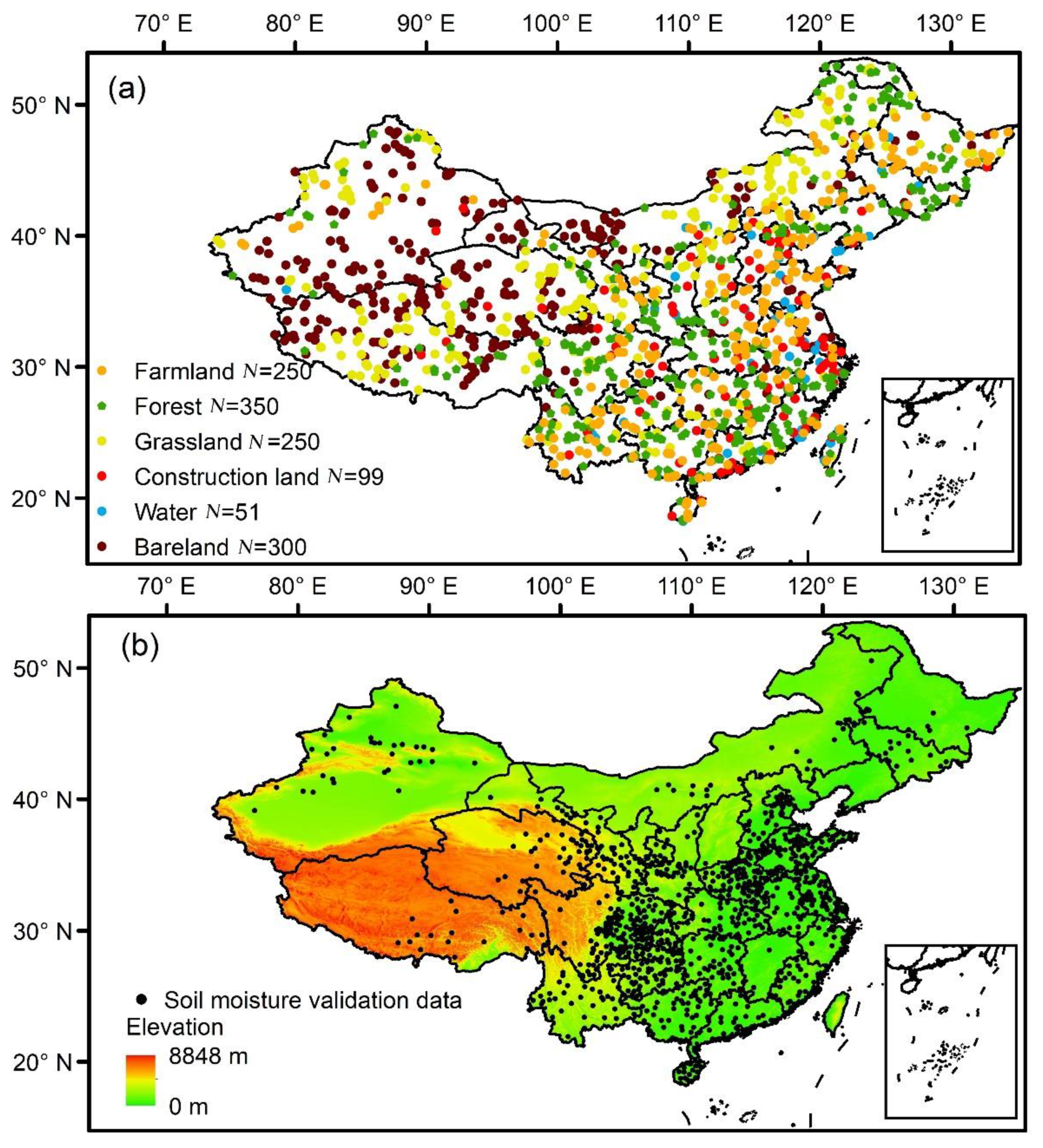
2.3.1. Land Cover Validation Data

The land cover validation data were obtained from a crowdsourcing tool called Geo-Wiki. Geo-Wiki is a global scale land cover in situ database based on Google Earth, which has been widely used for training land cover data, calibration, and validation [34]. To ensure the reliability of the sample data, we compared the Geo-Wiki sample data with the Google Earth image in 2015, and finally, 1300 sample points were selected by stratified random sampling according to the proportion of area of different land cover types (Figure 1a).

2.3.2. Soil Moisture Validation Data

The soil moisture verification data in 2014 were obtained from the China National Meteorological Information Center. When the soil temperature is below 0 °C, the water in the soil exists in both solid and liquid forms, which inhibits reliable observations by the instruments. As a result, soil moisture in situ measurements are often flagged as missing values during winter in cold regions. In order to ensure the accuracy of soil moisture validation data on the national scale, we selected 969 soil moisture stations at the depth of 10 cm with continuous observations from April to October in 2014, where soil temperatures at these stations were greater than 0 °C (Figure 1b).

2.4. Fusion Method Construction

We proposed a new fusion method to generate integrated land cover data for LSMs. We improved the D-S evidence theory through a mathematical model to deal with the issue of evidence conflicts, ensuring the stability of the D-S fusion method. In order to quantify the differences between different land cover classification systems, we further proposed a new knowledge rules method in the D-S fusion process. Our fusion method mainly consists of four steps (Figure 2): (1) construction of the frame of discernment, (2) construction of basic probability assignment based on knowledge rules, (3) fusion based on improved D-S evidence theory, and (4) establishment of decision rules.

2.4.1. Improving D-S Evidence Theory

The D-S evidence theory belongs to the category of artificial intelligence and has the capability of modeling uncertainty in input datasets [35]. The basic concept of evidence theory is the frame of discernment, denoted by Θ. The frame Θ is a collection of mutually incompatible elements. The basic probability assignment (BPA) function m ( A ) ( 0 , 1 ) in the frame Θ indicates the credibility of the evidence for the target A, where the sum of the basic probability values of all elements in the frame equals 1. The D-S evidence theory reflects the combined effect of evidences and is independent of the order of synthesis [36]. The D-S theory is implemented by orthogonal sum ( ) in mathematical expression. The fusion rules are as follows:
m 1 m 2 ( A ) = { 0       A = ϕ   A i   A j = m 1 ( A i ) m 2 ( A j ) 1 K   A ϕ  
K = A i   A j = ϕ m 1 ( A i ) m 2 ( A j )
where m1 and m2 are, respectively, BPA functions corresponding to the two evidence sources S1 and S2 under the frame Θ, and their target elements are Ai and Aj, respectively. ϕ is empty set. The conflict coefficient K is the extent of conflict between S1 and S2. A higher K indicates more conflict between the evidence. K 0 indicates that the fusion result is unreasonable, and K = 1 indicates that the synthetic rules are invalid.
Usually, the failure of D-S evidence theory fusion or contrary to the facts is caused by evidence conflicts [37], which are mainly divided into the following three cases. (1) Complete conflict: the conflict coefficient K equals 1, and the D-S fusion rule is invalid. (2) 0-paradox: among myriad evidence, if the BPA value of a certain evidence for target A is 0, the fusion result is still 0 for A, regardless of how high the BPA values of the other evidences for A are, which is contrary to the fact. (3) 1-paradox: when all the evidence has lower BPA values for the target A, but the fusion result is A, which is contrary to the fact. The shortcomings of D-S evidence theory are mainly improved by correcting the evidence or modifying the fusion rule. Here, we improved the algorithm by using mathematical models to modify the data sources. Supposing there is a frame of discernment Θ = {A1, A2, A3, ,At}, the BPA functions are denoted by {m1, m2, ,mn}, which correspond to the evidence source {S1, S2, ,Sn}. The sum of the BPA value is 1, and the average BPA value in the frame is 1/t. When the BPA values of an evidence source for all targets in the frame are 1/t, the evidence source fails to identify the target clearly. Therefore, 1/t can be used as a criterion for judging whether the target is credible. If the BPA value of a target is lower than this standard, the target recognition result is not credible. In accordance with the above principles, we have made the following corrections:
(1) Correct the BPA functions according to Equation (3):
m i ( A j ) = { e 2 m i ( A j ) 2 t m i ( A j ) <   1 t e 2 m i ( A j ) + 2 t m i ( A j ) 1 t
where m i ( A j ) represents the BPA function of the evidence source i for the target j.(2) Normalize the modified BPA value using Equation (4):
m i ( A j ) = m i ( A j ) j = 1 m m i ( A j )
(3) Fuse the normalized BPA value according to Equations (1) and (2).

2.4.2. Construction of the Frame of Discernment

The frame of discernment is the most basic concept in D-S evidence theory and involves the description of all concepts and functions in the theory. In the progress of multi-source land cover data fusion, the frame of discernment is the land cover classification system of the fusion result. The Noah-MP LSM adopts the USGS 24-category classification system [3]. Considering the distribution characteristics of vegetation in China and the spatial resolution adopted by the study, the study removed the savanna and tundra categories in the original classification system (Original code 10 and 20–23). These categories are sparsely distributed in China and difficult to form large-area distributions at the kilometer scale. Among the input data, only MODIS data has the land cover type of crop/natural vegetation mosaic, while other data are pure land type on the pixel scale. In order to ensure the reliability of the fusion result, the study removed the mosaic of different vegetation in the original classification system (original code 4–6 and 9). Finally, a frame of discernment with 15 land cover types was constructed (Table 1).

2.4.3. Construction of BPA Based on Knowledge Rules Optimization

The D-S evidence theory uses the BPA function to determine the support level of each initial category for each target category. Different land cover data have different accuracy in different land cover types because of different algorithm and data source. For example, TM/ETM+ images are used as data source for FROM-GLC, while MODIS images are used as data sources for MODIS LC. CNLULC are retrieved by visual interpretation method, while FROM-GLC are retrieved by multiple machine learning algorithm. Therefore, differences in algorithms and data sources ultimately lead to differences in the accuracy of land cover products. Moreover, different land cover data classification systems also have differences in the definition of categories. We considered the above factors to construct the following basic probability distribution function:
m i ( A j ) = P i R i ( A j ) C i j = 1 M P i R i ( A j ) C i
We supposed that there are N sets of land cover data that need to be merged into one land cover dataset with M land cover types. m i ( A j ) is an array with M elements, which represents the BPA value of the i-th land cover data for the j-th target land cover type on a pixel scale. Pi is the classification accuracy of the i-th land cover data on pixels. For the accuracy of different land cover products in different land cover types, we could obtain it by referring to the official product manuals of these products and related verification documents [30,31]. R i ( A j ) is an array with M elements that indicates the correlation between the i-th land cover data and the j-th target type on a pixel scale, which can be obtained by an affinity score. Ci represents the proportion of the optimal land cover type of pixels after resampling of the i-th land cover data.
Here, we adopted the method of knowledge rules optimization to score the affinity of the initial type to the target type by referring to the semantic correlation and differences between the initial type and the target type of different land cover data, such as environmental status, life form, leaf type, and leaf phenology. Affinity was divided into five scores within 0–100, where the score of “Is not” is 0, the score of “little related” is 25, the score of “partly related” is 50, the score of “mostly related” is 75, and the score of “Is” is 100. Although this kind of knowledge rule-based scoring has certain subjectivity, dividing the score into five grades by fuzzy processing can avoid the problem of scoring disaster and meet the needs of D-S algorithm fusion [21]. Table 2 shows an example of scoring rules.
Assuming that the initial land cover type in a land cover data is A and the land cover type in the target classification system is B, the affinity score between A and B is defined as follows based on the knowledge rule:
(1)
If A and B have no relationship in definition, such as “Water bodies” and “Urban and built-up land”, then the affinity score between A and B is 0.
(2)
If A and B are partly related, such as “evergreen mixed forest” and “evergreen green forest”, then the affinity score between A and B is 50.
(3)
If A and B are completely matched in definition, such as “evergreen mixed forest” and “mixed forest”, then the affinity score between A and B is 100.
(4)
If A and B are little or mostly related, then the affinity score between A and B is 25 or 75.

2.4.4. Establishment of Decision Rules Based on Degree of Belief

We established the BPA function by determining the frame of discernment and obtained the support probability of all the land cover types in the frame of discernment by using the improved D-S evidence theory. In order to finalize the land cover type for each pixel, the fusion results needed to be decided. The total degree of belief function was defined as follows:
B e l ( A ) = B A m ( B )
where Bel(A) is total degree of belief for target A on a pixel. In this study, the maximum total degree of belief was used as the decision rule. The total degree of belief all the land cover types output was compared, and the type with the maximum total belief was taken as the final fusion result. Finally, we obtained the China fusion land cover data (CFLC) for Noah-MP LSM in 2015

2.5. Soil Moisture Simulation Based on Noah-MP LSM

Noah-MP LSM is the currently widely used third-generation land surface model, which was developed by Yang Zongliang’s research group at the University of Texas at Austin (UT-Austin) [3]. It consists of 12 biophysical, biochemical, and hydrological processes on the basis of Noah-LSM, such as a short-term dynamic vegetation model, stomatal resistance, radiation transfer, and turbulent heat exchange. Each process also includes several parameterization schemes used in different land surface processes [38,39]. Here, we used the offline version of Noah-MP V1.6 with CLDAS V2.0 atmospheric forcing data in 2014, which is used by the China Meteorological Administration in the meteorological service system. The parameterized schemes adopted were dynamic vegetation and a modified two-stream radiation transmission scheme with other default schemes.
In order to compare the simulation effects of different land cover data, three sets of simulation experiments with different land cover data were designed. The first set of experiments used the USGS land cover data originally included in the model, denoted as USGS/SM. The second set of experiments used the currently widely used MODIS LC, denoted as MODIS/SM. The third set of experiments put the CFLC data generated in the study into the model, denoted as CFLC/SM. The three sets of experiments output the simulation results of soil moisture at the depth of 10 cm every 6 h (00:00, 06:00, 12:00, and 18:00 universal time). The spatial resolution of the simulation results is 0.0625°, which is consistent with the atmospheric forcing data. Considering that soil observations in north of China during winter were mostly invalid values, we selected the simulation results of 0–10 cm soil moisture in the growing season (from April to October) in 2014.
We mainly used three evaluation indicators: bias, root mean square error (RMSE), and correlation coefficient (R) to evaluate the results of Noah-MP soil moisture simulation. The calculation equations are as follows:
B i a s = 1 N i = 1 N ( S i G i )
R M S E = i = 1 N ( S i G i ) 2 n
R = i = 1 N ( S i S ¯ ) ( G i G ¯ ) i = 1 N ( S i S ¯ ) 2 i = 1 N ( G i G ¯ ) 2
where N is the number of samples, Gi is the observation data, Si is the simulation result, and G ¯ and S ¯ are the average values of observations and simulations.

3. Results

By establishing the fusion method based on improving D-S evidence theory and knowledge rules optimization, we combined CNLULC, MODIS LC, FROM-GLC, and China vegetation map to obtain the China fusion land cover data (CFLC) in 2015 for Noah-MP LSM (Figure 3). In order to facilitate the comparative analysis of the fusion result, the land cover classification system was integrated under a 6-class system according to the method proposed by Ran [30], including farmland (fusion code 2 and 3 in Table 1), forest (fusion code 5–9 in Table 1), grassland (fusion code 4 in Table 1), waters (fusion code 11–13 in Table 1), construction land (fusion code 1 in Table 1), and bare land (fusion code 14 and 15 in Table 1).

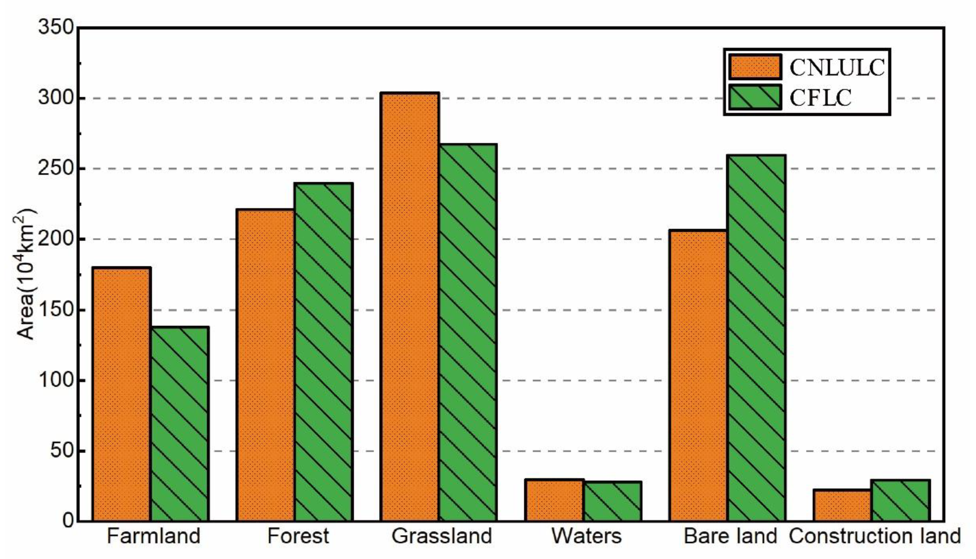
3.1. Comparison of CFLC and CNLULC

The differences of the area of each land cover type between the CFLC and CNLULC were calculated under a 6-class system in 2015 (Figure 4). We showed that the CFLC was basically consistent with the CNLULC in the total area of each type. The difference was mainly reflected in the decline in the farmland and grassland areas and the increase in the area of forest and bare land. By consulting the China Land and Resources Bulletin in 2016, we found that by the end of 2015, China had farmland of 1,349,987 km2, forest of 2,529,920 km2, and grassland of 2,194,206 km2. The farmland, forest, and grassland of CFLC were closer to the statistical data than that of CNLULC. The increase in bare land area was mainly due to the inclusion of some low-density vegetation in the bare land of the new classification system. Therefore, by analyzing the difference in the total area of the six classes, we found that the fusion result was reasonable with certain improvements in CNLULC.
The spatial differences were analyzed by establishing an error matrix (producer’s accuracy and omission error) between the CFLC and CNLULC. As shown in Table 3, the spatial consistency of forest, construction land, and bare land has reached more than 90%, followed by more than 80% of farmland. The spatial consistency of the waters and grassland was more than 70%, which was mainly due to the land type of herbaceous wetland added after the fusion, resulting in a relatively low spatial consistency. The overall spatial consistency of the fusion result was 84.5% at a Kappa coefficient of 0.796. Since CNLULC products were produced based on visual image interpretation, it can achieve 95% classification accuracy in China [29,30]. Therefore, the overall accuracy of the CFLC can reach 80.3% (84.5% × 95%). The CFLC maintained a classification accuracy of CNLULC, and also realized the conversion from the initial land cover classification system to the land cover classification system of Noah-MP, increasing detailed information such as land cover types of different forest and wetland.

3.2. Comparison of CFLC and Global Remote Sensing Land Cover Data

3.2.1. Comparison of Classification Accuracy Based on Geo-Wiki

We showed that both of the producer’s and user’s accuracy of CFLC was higher than that of the two global land cover data in all land cover classes except for waters, which was lower than MODIS LC (Table 4). The overall accuracy of the CFLC is 71.4% relative to GEO-WIKI observation (58.2% for FROM-GLC and 52.7% for MODIS). The main reason for the low accuracy of the waters in the CFLC was that the number of verification samples of waters was only 51, accounting for 3.94% of the total number of samples. A smaller number of samples cannot objectively evaluate the accuracy of the classification results for waters. Overall, the accuracy of CFLC was significantly higher than the other two global land cover data.

3.2.2. Cross-Validation Based on Multiple Land Cover Data

We calculated the relative consistency between MODIS LC, FROM-GLC, CNLULC, and CFLC, i.e., the consistency of spatial distribution of each two land cover data (Table 5). The low relative consistency between the three input data indicates that a single land cover product has great uncertainty in the simulation of LSMs. The relative consistency between the fusion results and the three input data is above 0.7, indicating that the fusion process had good compatibility with the rich feature information of three land cover data, which helps to reduce the uncertainty caused by a single data source. CFLC-CNLULC had the highest relative consistency, indicating that, in the process of fusion, CNLULC contributed more information to the fusion result than the other two global land cover data and had the greatest weight in the fusion process, inheriting the high precision of CNLULC.

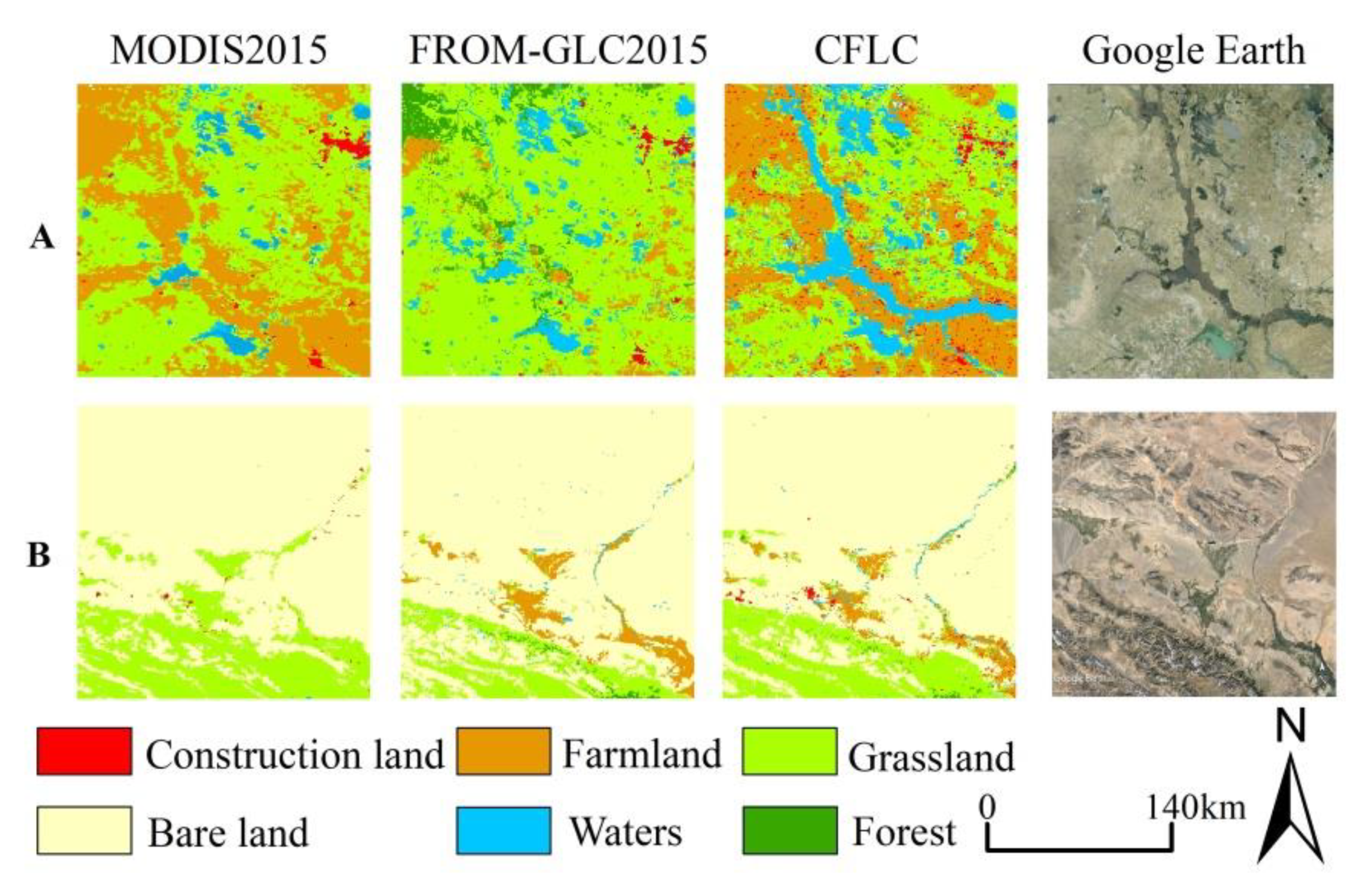
3.2.3. Comparison of Typical Areas

In order to intuitively compare the differences between MODIS LC, FROM-GLC, and CFLC, we selected two typical regions (Figure 5) for visual comparison. As shown in Figure 5, the three data basically reflected the overall land cover characteristics of the area, but there were some differences in the reflection of local detail features. In region A, MODIS LC identified the Nenjiang River as grassland. The FROM-GLC vaguely reflected a watercourse of the Nenjiang River, but a large amount of farmland in riverbanks was identified as grassland. CFLC clearly reflected the distribution of Nenjiang River and its surrounding farmland. In region B, all three data could show the outline of the Jinta Oasis. However, MODIS LC identified most area of oasis as grassland and lacked information on the Heihe River channel. FROM-GLC could clearly reflect the distribution of farmland in oasis, but it lacked the information on the construction land of the city. CFLC reflected the distribution of farmland and the construction land in Jinta Oasis and clearly showed the channel information of the Heihe River. Therefore, the CFLC was more compatible with the characteristics of the two global land cover data, and because it retained the accuracy of CNLULC, CFLC was more detailed and accurate when reflecting the detailed characteristics of local land cover.

3.3. Uncertainty Analysis

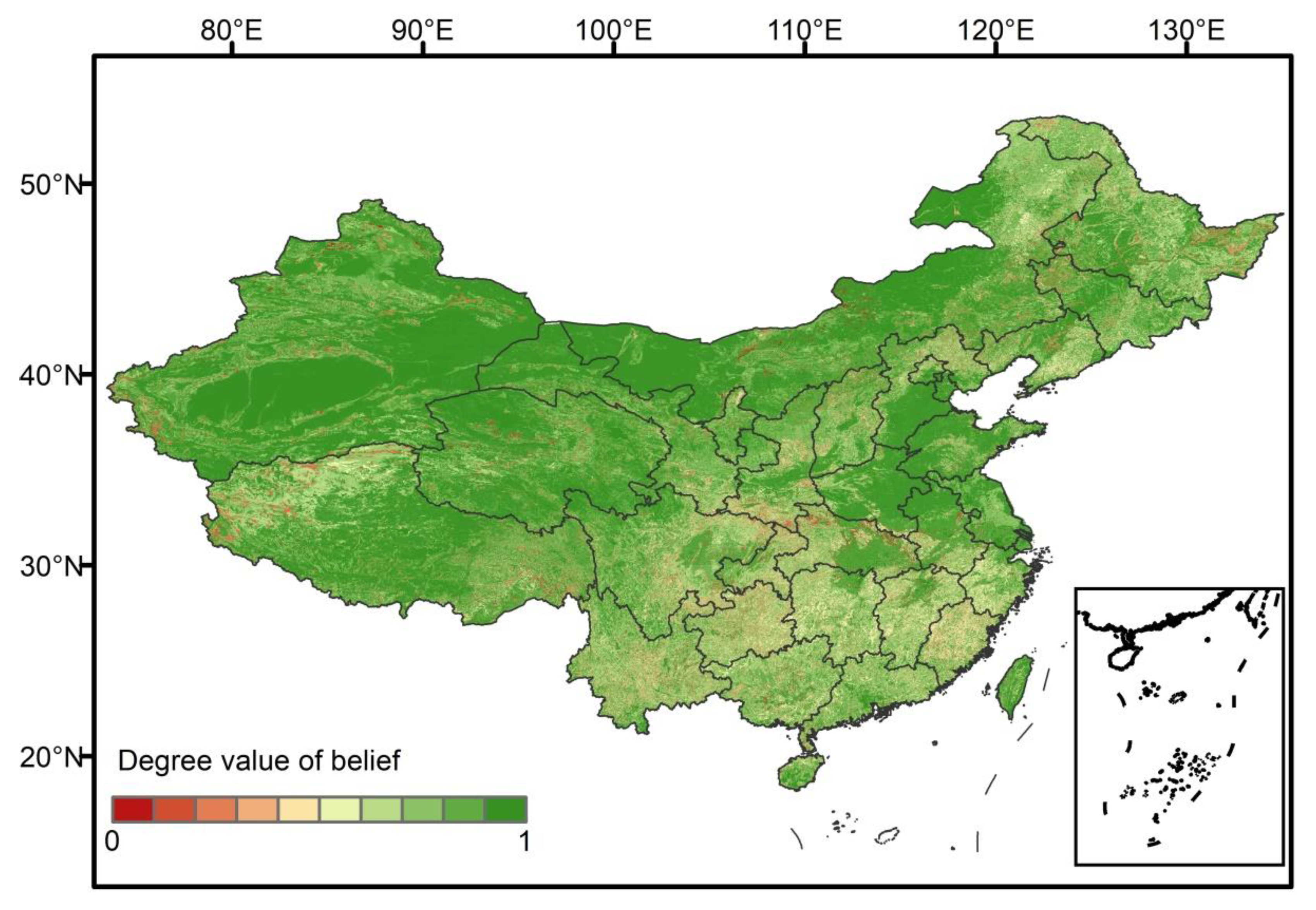
3.3.1. The Spatial Distribution of Certainty

According to the maximum degree of belief in the fusion process, the spatial distribution map of the certainty of CFLC on the national scale was constructed (Figure 6). The low degree of belief indicates the high uncertainty of the pixel. As shown in Figure 6, the certainty of the pixels in most of the northwestern region and the North China Plain was above 0.6. The high certainty in these regions was mainly due to the relatively homogeneous land cover. The northwestern region was dominated by bare land and grassland, while the North China Plain was dominated by dryland cropland. The areas with low certainty were mainly distributed in the southern hilly areas, the southwestern mountainous areas, and parts of the Qinghai–Tibet plateau. The complex climate environment and geographical condition of these regions made the land cover highly heterogeneous, leading to an increase in the uncertainty of CFLC.

3.3.2. The Certainty of Different Land Cover Types

We showed the distribution of degree of belief of different land cover types in the fusion process in Table 6. We found that the degree of belief of each type was greater than the basic probability that equaled 1/15, indicating that there was no failed pixel in the fusion process. Except for shrub land, herbaceous wetland, and wooden wetland, the average value of degree of belief was above 0.6, indicating that the overall uncertainty of these types was relatively low. The maximum value of these types was above 0.9, which indicates that CFLC had extremely high certainty in some areas. The average degree of belief of shrub land was around 0.5. The main reason is that different land cover data have different definitions of shrub coverage density and height, resulting in a non-uniform definition between forest, shrub, and grass, which increases uncertainty. The lower certainty of herbaceous wetland and wooden wetland was related to the lack of direct evidence for the input land cover data to support these two land cover types.

3.4. Analysis of Soil Moisture Simulation Based on Noah-MP LSM

Here, we designed three sets of experiments using different land cover data for soil moisture simulation according to the method in Section 3.3. We showed the difference of the area of each type between the initial land cover data (USGS LC) in Noah-MP and the land cover data generated in this study (CFLC) under a 6-class system in Table 7. More than a quarter of USGS LC was farmland, and nearly half of MODIS LC in China was grassland, which was unreasonable according to China Land and Resources Bulletin in 2016. In contrast, the distribution ratio of these features in CFLC was more reasonable. In addition, CFLC also improved the underestimation of open water and construction land area in USGS LC and MODIS LC.
Bias, root mean square error (RMSE), and correlation coefficient (R) were chosen to evaluate the reasonableness of the simulation results. Positive (negative) bias represents that simulation values are higher (lower) than the observed values. The higher R and lower RMSE indicate that the simulation results are closer to the observed values, i.e., the results are more reasonable. The simulated daily average soil moisture at the depth of 0–10 cm was calculated and bilinearly interpolated to the station. The significance level of simulation and observation data in this study is p < 0.01. As shown in Figure 7, there were obvious underestimations in USGS/SM, and the days of negative deviation accounted for 74.8%. MODIS/SM also had relatively more underestimations, which accounted for 65.4%. The improvement effect of CFLC on simulation was obvious, and the simulation results underestimate that the number of days accounted for 51.3%, which was the lowest among the three groups of experiments. The RMSE of the three sets of experiments generally fluctuated greatly from the 152nd to the 230th day, mainly because China was in the summer during this period, and the high precipitation frequency reduced the stability of the model simulation. The RMSE of CFLC/SM was the lowest, while the RMSE of MODIS/SM was relatively high, and the reason may be that this study converted MODIS LC to the land cover data required by the model using a widely used mapping relationship, which increased the uncertainty of the simulation. By analyzing the correlation coefficient, compared with USGS/SM and MODIS/SM, the correlation coefficient of CFLC/SM was generally higher, and the improvement effect was better. The correlation coefficients of the three sets of experiments were all greater than 0.6, and all passed the significance test of p < 0.01, but the model simulation was poor on the 274th to 304th days, which may be caused by the instability of the model itself. In addition, soil moisture tends to change gradually over a short distance due to its mobility in soil, which is greatly affected by external factors with strong heterogeneity, such as soil texture and topography. The site soil moisture obtained by Traditional interpolation methods such as bilinear interpolation and nearest neighbor interpolation was not accurate, which also reduced the overall correlation of the simulation results to a certain extent. In general, on the daily scale, the simulated soil moisture at the depth of 0–10 cm using CFLC was superior to the USGS LC and MODIS LC.1-1
In order to evaluate the influence of different land cover data on the spatial distribution of simulating 0–10 cm soil moisture, we calculated the spatial distribution of the RMSE of the daily mean soil moisture simulated by three sets of experiments relative to observation. As shown in Figure 8, the RMSE of the stations in the southwestern region is relatively high, possibly due to the complex topography and the diverse types of land cover in this area, resulting in strong spatial heterogeneity of soil moisture [40]. Moreover, the soil moisture of the stations obtained by interpolation cannot well represent the real soil moisture of the station. The three sets of experiments have good simulation results at most stations in eastern China, and the root mean square error is 0–0.1 m3/m3. Compared with USGS and MODIS LC, CFLC data have improved the stations with higher RMSE in the southwest region, and the number of stations with RMSE higher than 0.1 m3/m3 has been reduced. As shown in Figure 8d, for CFLC/SM, the number of sites with a RMSE higher than 0.1 accounted for 20.1%, which is reduced by 5.2% and 3.1% compared to USGS/SM and MODIS/SM, respectively. While for CFLC/SM, the number of sites with RMSE lower than 0.05 accounted for 29.2%, which is increased by 6.7% and 7.5% compared to USGS/SM and MODIS/SM, respectively. Overall, the simulated soil moisture at the depth of 0–10 cm by CFLC was superior to the USGS LC and MDOIS LC by spatial station analysis.

4. Discussion

Considering that land cover products are often not specifically designed and produced for LSMs or other numerical models, it is difficult for a single land cover datum to meet the usage requirements of models in classification systems, category definitions, and space-time resolution of land features. In this study, a new land cover data fusion method was established by improving D-S evidence theory with mathematical models and knowledge rules optimization. We showed that CFLC in 2015 generated by a new method had more abundant land cover classes than visual interpretation-based CNLULC data and higher accuracy relative to two global land cover data (MODIS LC and FROM-GLC).
CNLULC data generated by visual interpretation are widely used in the fields of environment, ecology, and meteorology due to their high accuracy at the national scale. However, CNLULC lacks descriptions of vegetation characteristics such as phenology and leaf shape, which limits further application in LSMs. Here, we provided CNLULC with more abundant land cover classes to meet the needs of LSMs by integrating multiple global land cover products. Our verifications showed that the fusion results retain the high-precision features of CNLULC and enrich the original land cover classes of CNLULC to meet the needs of LSMs.
Currently, studying the physical and biochemical processes between various underlying surfaces and the atmosphere–land, and further developing advanced LSMs have become an urgent need for global change research. High-quality land cover data provide accurate underlying surface information for LSMs to improve model simulation. Most previous studies aimed to assess the impact of different land cover data on model simulations [41,42]. However, the physical definition, accuracy, and resolution of single-source land-cover data are subject to great uncertainty, making it difficult to find a set of land-cover products suitable for LSM simulation at the national scale. Here, we generated high-quality land cover data for the Noah-MP LSM by fusing multiple land cover data, reducing the uncertainty of a single set of land cover data with a great potential to improve the accuracy of simulations.
The traditional D-S evidence theory is widely used in the fusion of uncertain information [36,37]. However, fusion failures also occur when faced with severe disagreement information. Here, we used the mathematical model method to improve the traditional D-S evidence theory, so that it has the ability to deal with serious disagreement information, thereby improving the robustness of the theory. Although this study only generated land cover data in 2015, our method is still highly portable and generalizable, which means that more land cover data, such as ESA CCI 300 m Land Cover data and newly released ESA WorldCover 10 m land cover data, can be fused by our method to generate higher accuracy and long time series comprehensive land cover data with a specific land cover classification system for LSMs. Our new method provides a new approach to land cover mapping for LSMs. In addition, different fields such as ecological environment, land management, and agricultural management require land cover data of specific classification systems, and current global land cover products may not meet the requirements of a certain field. The fusion method proposed in this paper makes it possible to develop land cover data for different fields.
Although the new fusion method improved multiple input data, the uncertainty analysis showed that the fusion effect can be affected by the following sources: (1) the uncertainty of the input data. The classification accuracy of land cover data is heterogeneous in space, which is mainly reflected in the fact that different land cover types in the same area have different classification accuracy and the same land cover type has different classification accuracy in different areas. This study obtained the classification accuracy of these products through literature reviews or product manuals, which only considered the overall classification accuracy of each land cover type within a particular area, which is probably the most important source of uncertainty in the CFLC map [16,30]. (2) The uncertainty of affinity score. To construct the BPA function, it is important to score the affinity between the input land cover system and the target land cover system. When all input data do not have significant correlations with a specific target type, this could result in a low and fuzzy affinity score for that specific target type, which is another source of uncertainty in the CFLC map. For example, there is no definition directly related to the target category of woody wetland in the input data, which increases the uncertainty of the fusion result.
The land cover data for LSMs can be directly produced by remote sensing interpretation, or by multi-source remote sensing data based on pixel level fusion or feature level fusion to absorb the advantages of different remote sensing data, which is often costly, requiring lots of research and human resources. Here, our method obtained new land cover data for LSMs by fusion of currently mature remote sensing land cover products based on decision-level fusion, which is efficient and easy to implement. However, there are still some limitations of our fusion method. Due to the different classification systems and category physical definitions of different remote sensing data products, researchers need to have a deeper understanding of the similarities and differences between different land cover categories to realize the construction of BPA function based on knowledge rules optimization. One of the potential solutions to the above problem is to establish a semantic analysis system based on artificial natural language to reduce the influence of human subjectivity on fusion process. The uncertainty of the input land cover data may also affect the reliability of the fusion result, which requires more field survey data and high-resolution remote sensing images to verify in the future. Moreover, this study evaluated the spatial distribution of fusion results only by visual comparison, more reliable methods are needed for quantitative evaluation in future research. Overall, the research on land cover data fusion for LSMs is a challenging task, requiring fusion of the advantages of different data while maintaining classification accuracy, and consistent with the physical definitions of the land cover category required by the LSM to meet the requirements of model operation. This research explored the above-mentioned scientific issues to a certain extent. With the development of remote sensing land cover data and the advancement of artificial intelligence semantic analysis technology in the future, our methods will continue to be improved. In addition, limited by computing costs, this study only evaluated the simulation effect of the new land cover data on soil moisture to verify the superiority of our new method. However, the land cover data can also affect the simulation of land surface parameters such as land surface temperature and soil temperature [5,43], which need to be fully evaluated in future research.

5. Conclusions

High accurate land cover data can significantly ensure the accuracy of LSM simulation. Currently, the widely used global remote sensing land cover products cannot meet the requirements of land surface models (LSMs) for classification systems, physical definition, data accuracy, and space-time resolution. In this study, we proposed a new method to generate integrated land cover data for LSMs. The conclusions of our research are as follows:
(1)
A new land cover data fusion method was established by improving D-S evidence theory with mathematical models and knowledge rules optimization. The new method can reduce the contradiction between input data and realize the conversion of multiple land cover classification systems to the Noah-MP classification system.
(2)
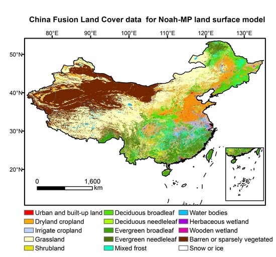
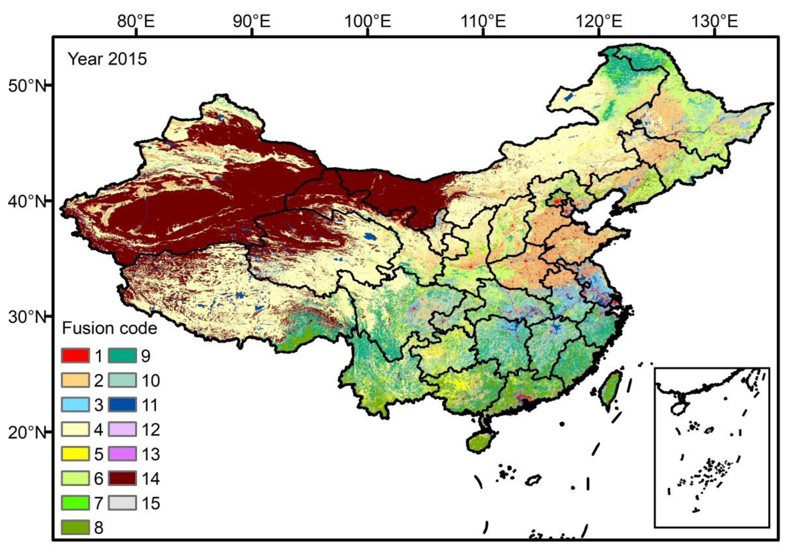
Measured data verification and visual comparisons showed that China Fusion Land Cover data (CFLC) in 2015 generated by new method had more abundant land cover classes than visual interpretation-based CNLULC data and higher accuracy relative to two global land cover data (MODIS LC and FROM-GLC). Compared with Geo-Wiki observations in 2015, the overall accuracy for CFLC is 71.4% relative to other two global land cover data (58.2% for FROM-GLC and 52.7% for MODIS).
(3)
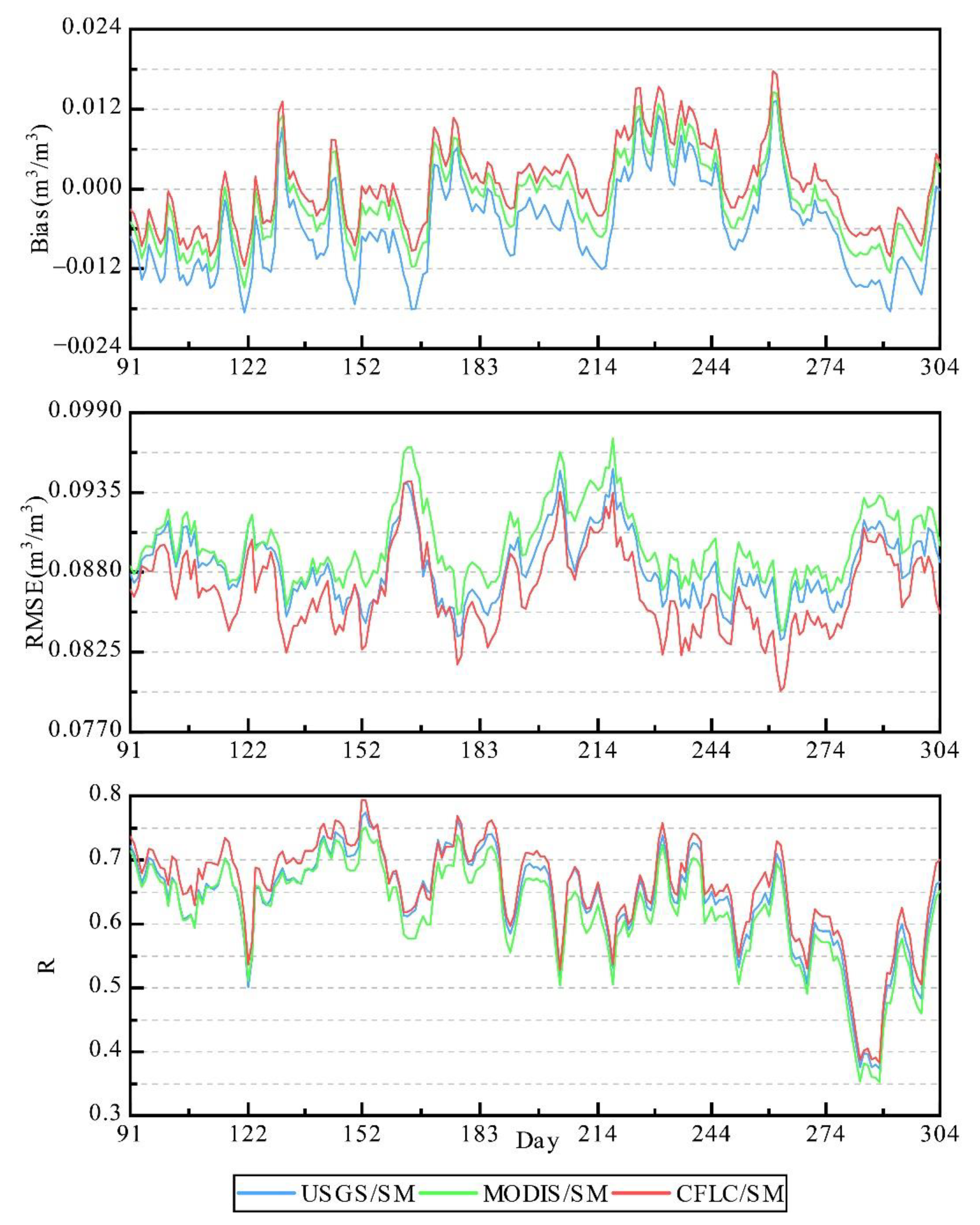
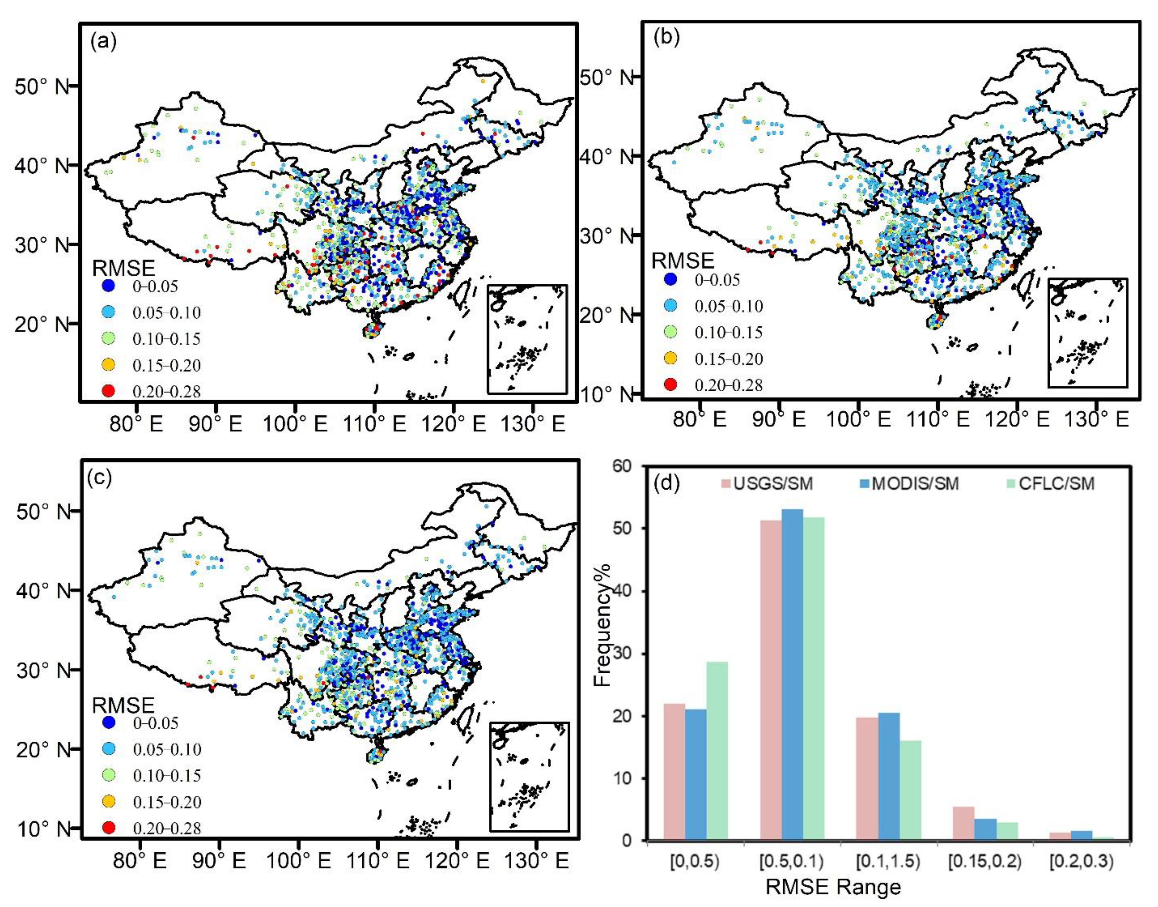
The site-based evaluation results showed that the new integrated land cover data improved the simulation accuracy of soil moisture at the depth of 10 cm in Noah-MP LSM relative to the initial land cover data in the model and widely used MODIS land cover data. The underestimation rate was reduced by 23.5% and 14.1% relative to initial land cover data and MODIS land cover data, respectively, while the correlation coefficient and the root mean square error of the soil moisture simulated by the CFLC were all better than that simulated by the initial land cover data in the model and widely used MODIS land cover data.

Author Contributions

A.H.: Conceptualization, methodology, formal analysis, Writing—Original draft, Writing—Review and Editing. R.S.: Conceptualization, Supervision, Writing—Review and Editing. Y.L.: Investigation, Formal Analysis, Writing. H.H.: Investigation, Data Curation, Writing—Original Draft. W.D.: Software, Visualization. D.F.T.H.: Writing—Review and Editing. All authors have read and agreed to the published version of the manuscript.

Funding

This research was funded by the National Key R&D Program of China (Grant number 2018YFC1506602), the Key Project of the National Natural Science Foundation of China (Grant number 91437220) and Undergraduate Innovation Training Program of Nanjing University of Information Science and Technology (Grant number 201910300170).

Institutional Review Board Statement

Not applicable.

Informed Consent Statement

Not applicable.

Data Availability Statement

MODIS land cover data (MCD12Q1 version 6) is openly available in the Land Processes Distributed Active Archive Center at https://doi.org/10.5067/MODIS/MCD12Q1.006 (accessed on 1 December 2021). FROM-GLC land cover data is openly available in Tsinghua University at http://data.ess.tsinghua.edu.cn (accessed on 1 December 2021). China land use map and China vegetation map are openly available in the Resource and Environmental Science Data Center of the Chinese Academy of Sciences at https://www.resdc.cn (accessed on 1 December 2021). Atmospheric forcing data obtained from the China land data assimilation system version 2.0 (CLDAS V2.0) developed by the China National Meteorological Information Center (CMA) in http://data.cma.cn (accessed on 1 December 2021).

Acknowledgments

This research was supported by the National Key R&D Program of China (Grant number 2018YFC1506602), the Key Project of the National Natural Science Foundation of China (Grant number 91437220) and Undergraduate Innovation Training Program of Nanjing University of Information Science and Technology (Grant number 201910300170). We are grateful to the High Performance Computing Centre of Nanjing University of Information Science and Technology for doing the numerical calculations in this study on its blade cluster system.

Conflicts of Interest

The authors declare no conflict of interest.

References

  1. Sellers, P.J.; Tucker, C.J.; Collatz, G.J.; Los, S.O.; Justice, C.O.; Dazlich, D.A.; Randall, D.A. A revised land surface parameterization (SiB2) for atmospheric GCMs. Part II: The generation of global fields of terrestrial biophysical parameters from satellite data. J. Clim. 1996, 9, 706–737. [Google Scholar] [CrossRef] [Green Version]
  2. Dai, Y.; Zeng, X.; Dickinson, R.E.; Baker, I.; Bonan, G.B.; Bosilovich, M.G.; Denning, A.S.; Dirmeyer, P.A.; Houser, P.R.; Niu, G. The common land model. Bull. Am. Meteorol. Soc. 2003, 84, 1013–1024. [Google Scholar] [CrossRef] [Green Version]
  3. Yang, Z.L.; Niu, G.Y.; Mitchell, K.E.; Chen, F.; Ek, M.B.; Barlage, M.; Longuevergne, L.; Manning, K.; Niyogi, D.; Tewari, M. The community Noah land surface model with multiparameterization options (Noah-MP): 2. Evaluation over global river basins. J. Geophys. Res. Atmos. 2011, 116, D12. [Google Scholar] [CrossRef]
  4. Niraula, R.; Meixner, T.; Norman, L.M. Determining the importance of model calibration for forecasting absolute/relative changes in streamflow from LULC and climate changes. J. Hydrol. 2015, 522, 439–451. [Google Scholar] [CrossRef]
  5. Chen, C.; Li, D.; Li, Y.; Piao, S.; Wang, X.; Huang, M.; Gentine, P.; Nemani, R.R.; Myneni, R.B. Biophysical impacts of Earth greening largely controlled by aerodynamic resistance. Sci. Adv. 2020, 6, eabb1981. [Google Scholar] [CrossRef]
  6. Ge, J.; Pitman, A.J.; Guo, W.; Wang, S.; Fu, C. Do uncertainties in the reconstruction of land cover affect the simulation of air temperature and rainfall in the CORDEX region of East Asia? J. Geophys. Res. Atmos. 2019, 124, 3647–3670. [Google Scholar] [CrossRef]
  7. Hansen, M.C.; Reed, B. A comparison of the IGBP DISCover and University of Maryland 1 km global land cover products. Int. J. Remote Sens. 2000, 21, 1365–1373. [Google Scholar] [CrossRef]
  8. Sulla-Menashe, D.; Gray, J.M.; Abercrombie, S.P.; Friedl, M.A. Hierarchical mapping of annual global land cover 2001 to present: The MODIS Collection 6 Land Cover product. Remote Sens. Environ. 2019, 222, 183–194. [Google Scholar] [CrossRef]
  9. Arino, O.; Gross, D.; Ranera, F.; Leroy, M.; Bicheron, P.; Brockman, C.; Defourny, P.; Vancutsem, C.; Achard, F.; Durieux, L. GlobCover: ESA service for global land cover from MERIS. In Proceedings of the 2007 IEEE International Geoscience and Remote Sensing Symposium, Barcelona, Spain, 23–27 July 2007; pp. 2412–2415. [Google Scholar]
  10. Chirachawala, C.; Shrestha, S.; Babel, M.S.; Virdis, S.G.; Wichakul, S. Evaluation of global land use/land cover products for hydrologic simulation in the Upper Yom River Basin, Thailand. Sci. Total Environ. 2020, 708, 135148. [Google Scholar] [CrossRef]
  11. Liang, L.; Liu, Q.; Liu, G.; Li, H.; Huang, C. Accuracy evaluation and consistency analysis of four global land cover products in the Arctic region. Remote Sens. 2019, 11, 1396. [Google Scholar] [CrossRef] [Green Version]
  12. Shi, W.; Zhang, X.; Hao, M.; Shao, P.; Cai, L.; Lyu, X. Validation of land cover products using reliability evaluation methods. Remote Sens. 2015, 7, 7846–7864. [Google Scholar] [CrossRef] [Green Version]
  13. Chen, B.; Huang, B.; Xu, B. Multi-source remotely sensed data fusion for improving land cover classification. ISPRS J. Photogramm. Remote Sens. 2017, 124, 27–39. [Google Scholar] [CrossRef]
  14. Ghassemian, H. A review of remote sensing image fusion methods. Inf. Fusion 2016, 32, 75–89. [Google Scholar] [CrossRef]
  15. Zhang, J. Multi-source remote sensing data fusion: Status and trends. Int. J. Image Data Fusion 2010, 1, 5–24. [Google Scholar] [CrossRef] [Green Version]
  16. Pérez-Hoyos, A.; García-Haro, F.J.; San-Miguel-Ayanz, J. A methodology to generate a synergetic land-cover map by fusion of different land-cover products. Int. J. Appl. Earth Obs. Geoinf. 2012, 19, 72–87. [Google Scholar] [CrossRef]
  17. Jung, M.; Henkel, K.; Herold, M.; Churkina, G. Exploiting synergies of global land cover products for carbon cycle modeling. Remote Sens. Environ. 2006, 101, 534–553. [Google Scholar] [CrossRef]
  18. See, L.; Schepaschenko, D.; Lesiv, M.; McCallum, I.; Fritz, S.; Comber, A.; Perger, C.; Schill, C.; Zhao, Y.; Maus, V. Building a hybrid land cover map with crowdsourcing and geographically weighted regression. ISPRS J. Photogramm. Remote Sens. 2015, 103, 48–56. [Google Scholar] [CrossRef] [Green Version]
  19. Gao, H.; Jia, G.; Fu, Y. Generate Integrated Land Cover Product for Regional Climate Model by Fusing Different Land Cover Products. In Proceedings of the International Conference on Collaborative Computing: Networking, Applications and Worksharing, Beijing, China, 16–17 October 2016; pp. 665–675. [Google Scholar]
  20. Liu, K.; Xu, E. Fusion and Correction of Multi-Source Land Cover Products Based on Spatial Detection and Uncertainty Reasoning Methods in Central Asia. Remote Sens. 2021, 13, 244. [Google Scholar] [CrossRef]
  21. Feng, M.; Bai, Y. A global land cover map produced through integrating multi-source datasets. Big Earth Data 2019, 3, 191–219. [Google Scholar] [CrossRef] [Green Version]
  22. Lesiv, M.; Moltchanova, E.; Schepaschenko, D.; See, L.; Shvidenko, A.; Comber, A.; Fritz, S. Comparison of data fusion methods using crowdsourced data in creating a hybrid forest cover map. Remote Sens. 2016, 8, 261. [Google Scholar] [CrossRef] [Green Version]
  23. Clinton, N.; Yu, L.; Gong, P. Geographic stacking: Decision fusion to increase global land cover map accuracy. ISPRS J. Photogramm. Remote Sens. 2015, 103, 57–65. [Google Scholar] [CrossRef]
  24. Kussul, N.; Shelestov, A.; Lavreniuk, M.; Butko, I.; Skakun, S. Deep learning approach for large scale land cover mapping based on remote sensing data fusion. In Proceedings of the 2016 IEEE International Geoscience and Remote Sensing Symposium (IGARSS), Beijing, China, 10–15 July 2016; pp. 198–201. [Google Scholar]
  25. Song, X.-P.; Huang, C.; Townshend, J.R. Improving global land cover characterization through data fusion. Geo-Spat. Inf. Sci. 2017, 20, 141–150. [Google Scholar] [CrossRef] [Green Version]
  26. Liu, Y.; Chen, X.; Wang, Z.; Wang, Z.J.; Ward, R.K.; Wang, X. Deep learning for pixel-level image fusion: Recent advances and future prospects. Inf. Fusion 2018, 42, 158–173. [Google Scholar] [CrossRef]
  27. Reichstein, M.; Camps-Valls, G.; Stevens, B.; Jung, M.; Denzler, J.; Carvalhais, N. Deep learning and process understanding for data-driven Earth system science. Nature 2019, 566, 195–204. [Google Scholar] [CrossRef] [PubMed]
  28. Han, S.; Shi, C.; Xu, B.; Sun, S.; Zhang, T.; Jiang, L.; Liang, X. Development and evaluation of hourly and kilometer resolution retrospective and real-time surface meteorological blended forcing dataset (smbfd) in china. J. Meteorol. Res. 2019, 33, 1168–1181. [Google Scholar] [CrossRef]
  29. Liu, J.; Liu, M.; Tian, H.; Zhuang, D.; Zhang, Z.; Zhang, W.; Tang, X.; Deng, X. Spatial and temporal patterns of China’s cropland during 1990–2000: An analysis based on Landsat TM data. Remote Sens. Environ. 2005, 98, 442–456. [Google Scholar] [CrossRef]
  30. Ran, Y.; Li, X.; Lu, L.; Li, Z. Large-scale land cover mapping with the integration of multi-source information based on the Dempster–Shafer theory. Int. J. Geogr. Inf. Sci. 2012, 26, 169–191. [Google Scholar] [CrossRef]
  31. Gong, P.; Wang, J.; Yu, L.; Zhao, Y.; Zhao, Y.; Liang, L.; Niu, Z.; Huang, X.; Fu, H.; Liu, S. Finer resolution observation and monitoring of global land cover: First mapping results with Landsat TM and ETM+ data. Int. J. Remote Sens. 2013, 34, 2607–2654. [Google Scholar] [CrossRef] [Green Version]
  32. Shi, C.; Xie, Z.; Qian, H.; Liang, M.; Yang, X. China land soil moisture EnKF data assimilation based on satellite remote sensing data. Sci. China Earth Sci. 2011, 54, 1430–1440. [Google Scholar] [CrossRef]
  33. Liu, J.; Shi, C.; Sun, S.; Liang, J.; Yang, Z.-L. Improving land surface hydrological simulations in China using CLDAS meteorological forcing data. J. Meteorol. Res. 2019, 33, 1194–1206. [Google Scholar] [CrossRef]
  34. Fritz, S.; McCallum, I.; Schill, C.; Perger, C.; See, L.; Schepaschenko, D.; Van der Velde, M.; Kraxner, F.; Obersteiner, M. Geo-Wiki: An online platform for improving global land cover. Environ. Model. Softw. 2012, 31, 110–123. [Google Scholar] [CrossRef]
  35. Jiang, W.; Zhan, J. A modified combination rule in generalized evidence theory. Appl. Intell. 2017, 46, 630–640. [Google Scholar] [CrossRef]
  36. Zhao, J.; Liu, S.; Wan, J.; Yasir, M.; Li, H. Change Detection Method of High Resolution Remote Sensing Image Based on DS Evidence Theory Feature Fusion. IEEE Access 2020, 9, 4673–4687. [Google Scholar] [CrossRef]
  37. Shafer, G. A betting interpretation for probabilities and Dempster-Shafer degrees of belief. arXiv 2010, arXiv:1001.1653. [Google Scholar] [CrossRef] [Green Version]
  38. Chang, M.; Liao, W.; Wang, X.; Zhang, Q.; Chen, W.; Wu, Z.; Hu, Z. An optimal ensemble of the Noah-MP land surface model for simulating surface heat fluxes over a typical subtropical forest in South China. Agric. For. Meteorol. 2020, 281, 107815. [Google Scholar] [CrossRef]
  39. Niu, G.Y.; Yang, Z.L.; Mitchell, K.E.; Chen, F.; Ek, M.B.; Barlage, M.; Kumar, A.; Manning, K.; Niyogi, D.; Rosero, E. The community Noah land surface model with multiparameterization options (Noah-MP): 1. Model description and evaluation with local-scale measurements. J. Geophys. Res. Atmos. 2011, 116, D12. [Google Scholar] [CrossRef] [Green Version]
  40. Hagan, D.F.T.; Parinussa, R.M.; Wang, G.; Draper, C.S. An Evaluation of Soil Moisture Anomalies from Global Model-Based Datasets over the People’s Republic of China. Water 2020, 12, 117. [Google Scholar] [CrossRef] [Green Version]
  41. Li, H.; Wolter, M.; Wang, X.; Sodoudi, S. Impact of land cover data on the simulation of urban heat island for Berlin using WRF coupled with bulk approach of Noah-LSM. Theor. Appl. Climatol. 2018, 134, 67–81. [Google Scholar] [CrossRef]
  42. Li, J.; Chen, F.; Zhang, G.; Barlage, M.; Gan, Y.; Xin, Y.; Wang, C. Impacts of land cover and soil texture uncertainty on land model simulations over the central Tibetan Plateau. J. Adv. Modeling Earth Syst. 2018, 10, 2121–2146. [Google Scholar] [CrossRef] [Green Version]
  43. Duveiller, G.; Caporaso, L.; Abad-Viñas, R.; Perugini, L.; Grassi, G.; Arneth, A.; Cescatti, A. Local biophysical effects of land use and land cover change: Towards an assessment tool for policy makers. Land Use Policy 2020, 91, 104382. [Google Scholar] [CrossRef]
Figure 1. Spatial distribution of the validation data. (a) The spatial distribution of land cover validation data. N represents the number of samples. (b) The spatial distribution of soil moisture validation sites.
Remotesensing 14 00972 g001
Figure 2. The flow chart of the fusion process.
Remotesensing 14 00972 g002
Figure 3. China fusion land cover data in 2015 for Noah-MP LSM.
Remotesensing 14 00972 g003
Figure 4. Comparison of total area of 6 classes between the CFLC and CNLULC.
Remotesensing 14 00972 g004
Figure 5. Local differences among the three land cover maps. The region (A) is located in Nenjiang River basin in Qiqihaer with a central coordinate of 124.21°E and 45.99°N, and the region (B) is located in Jinta County in the Heihe River Basin in Northwest of China, with central coordinates of 98.87°E, 40.24°N.
Remotesensing 14 00972 g005
Figure 6. Spatial distribution map of degree value of certainty in 2015.
Remotesensing 14 00972 g006
Figure 7. Daily scale analysis of 0–10 cm soil moisture between simulation result and observation. The significance level of all the data is p < 0.01.
Remotesensing 14 00972 g007
Figure 8. The spatial distribution map of the root mean square error of the daily mean soil moisture of 0–10 cm in 2014 simulated by Noah-MP. (a) The result of USGS/SM simulation. (b) The result of MODIS/SM simulation. (c) The result of CFLC/SM simulation. (d) The percentage of the root mean square error in different intervals.
Remotesensing 14 00972 g008
Table 1. The frame of discernment adopted in the study area.
Fusion CodeUSGS CodeLand Cover Type
11Urban and built-up land
22Dryland cropland and pasture
33Irrigated cropland and pasture
-4Mixed Dryland/Irrigated Cropland and Pasture
-5Cropland/Grassland Mosaic
-6Cropland/Woodland Mosaic
47Grassland
58Shrubland
-9Mixed Shrubland/Grassland
-10Savanna
611Deciduous broadleaf forest
712Deciduous needleleaf forest
813Evergreen broadleaf forest
914Evergreen needleleaf forest
1015Mixed forest
1116Water bodies
1217Herbaceous wetland
1318Wooden wetland
1419Barren or sparsely vegetable
-20Herbaceous Tundra
-21Wooded Tundra
-22Mixed Tundra
-23Bare Ground Tundra
1524Snow or ice
Table 2. Example of affinity score.
Initial TypeSemantic RuleScoreTarget Type
FROM-GLC
Mixed leaf, leaf-on
Is not0Water bodies
little related25Shrubland
partly related50Evergreen needle/broadleaf
mostly related75-
Is100Mixed forest
MODIS LC
Savannas
Is not0Water bodies
little related25Various types of forest
partly related50-
mostly related75Grassland
Is100-
Table 3. The error matrix of the CFLC and CNLULC under a 6-class system.
CFLCCNLULC
FarmlandForestGrasslandWatersConstruction LandBare Land
Farmland0.8010.0220.0150.0380.0050.003
Forest0.1020.9040.0500.03700.005
Grassland0.0910.0680.7900.15200.090
Waters0.0030.0020.0020.75000.002
Construction land00000.9940
Bare land0.0030.0040.1430.0230.0010.900
Overall accuracy = 84.5% Kappa = 0.796.
Table 4. Comparison of classification accuracy based on Geo-Wiki.
DataFarmlandForestGrasslandWatersConstruction LandBare Land
Producer’s
accuracy
CFLC0.8440.7740.8080.5100.7070.687
FROM-GLC0.7680.6340.5760.2350.1310.607
MODIS0.5680.3770.4760.6080.3930.483
User’s
accuracy
CFLC0.8180.8530.6590.2660.7660.950
FROM-GLC0.6440.6850.5890.3810.3500.744
MODIS0.5430.5850.4780.7240.5060.662
Table 5. The relative consistency between different land cover data.
Pair of DatasetsThe Relative Consistency
MODIS-FROMGLC0.648
MODIS-CNLULC0.587
MODIS-CFLC0.710
FROMGLC-CNLULC0.637
FROMGLC-CFLC0.756
CFLC-CNLULC0.845
Table 6. Distribution of certainty values across land cover types.
Land Cover TypeMinMaxRangeMean
Urban and built-up land0.2110.9960.7850.955
Dryland cropland and pasture0.1110.9910.8800.774
Irrigated cropland and pasture0.1850.9540.7690.669
Grassland0.1170.9900.8730.811
Shrubland0.1290.9860.8570.538
Deciduous broadleaf forest0.1100.9890.8790.676
Deciduous needleleaf forest0.1490.9550.8060.658
Evergreen broadleaf forest0.1540.9890.8350.620
Evergreen needleleaf forest0.1750.9890.8140.608
Mixed forest0.1670.9740.8070.642
Water bodies0.1250.9860.8610.965
Herbaceous wetland0.1150.8310.7160.557
Wooden wetland0.1240.4360.3120.306
Barren or sparsely vegetable0.1290.9950.8660.889
Snow or ice0.1650.9800.8150.771
Table 7. The proportion of land cover types under a 6-class system between 3 data.
FarmlandForestGrasslandWatersConstruction LandBare Land
USGS26.2%29.4%25.0%1.0%0. 1%18.3%
MODIS15.7%11.4%46.1%1.1%1.2%24.5%
CFLC14.3%24.9%27.8%2.9%3.0%27.0%
Publisher’s Note: MDPI stays neutral with regard to jurisdictional claims in published maps and institutional affiliations.

