Article

A Comparative Study of Convolutional Neural Networks and Conventional Machine Learning Models for Lithological Mapping Using Remote Sensing Data

1
School of Mining Engineering, College of Engineering, University of Tehran, Tehran P.O. Box 11155-4563, Iran
2
EarthByte Group, School of Geosciences, University of Sydney, Sydney, NSW 2006, Australia
3
Department of Mining Engineering, Amirkabir University of Technology (Tehran Polytechnic), Tehran P.O. Box 15875-4413, Iran
4
Institute of Oceanography and Environment (INOS), Universiti Malaysia Terengganu (UMT), Kuala Nerus 21030, Terengganu, Malaysia
5
The Centre for Advanced Modelling and Geospatial Information Systems (CAMGIS), School of Civil and Environmental Engineering, Faculty of Engineering and IT, University of Technology Sydney, Sydney, NSW 2007, Australia
6
Center of Excellence for Climate Change Research, King Abdulaziz University, P.O. Box 80234, Jeddah 21589, Saudi Arabia
7
Earth Observation Centre, Institute of Climate Change, Universiti Kebangsaan Malaysia, Bangi 43600, Selangor, Malaysia
8
UNSW Data Science Hub & School of Mathematics and Statistics, University of New South Wales, Sydney, NSW 2052, Australia
9
Data Analytics for Resources and Environments, Australian Research Council—Industrial Transformation Training Centre, Canberra, NSW 2052, Australia
*
Author to whom correspondence should be addressed.
Remote Sens. 2022, 14(4), 819; https://doi.org/10.3390/rs14040819
Submission received: 21 November 2021 / Revised: 2 February 2022 / Accepted: 5 February 2022 / Published: 9 February 2022

Abstract

:
Lithological mapping is a critical aspect of geological mapping that can be useful in studying the mineralization potential of a region and has implications for mineral prospectivity mapping. This is a challenging task if performed manually, particularly in highly remote areas that require a large number of participants and resources. The combination of machine learning (ML) methods and remote sensing data can provide a quick, low-cost, and accurate approach for mapping lithological units. This study used deep learning via convolutional neural networks and conventional ML methods involving support vector machines and multilayer perceptron to map lithological units of a mineral-rich area in the southeast of Iran. Moreover, we used and compared the efficiency of three different types of multispectral remote-sensing data, including Landsat 8 operational land imager (OLI), advanced spaceborne thermal emission and reflection radiometer (ASTER), and Sentinel-2. The results show that CNNs and conventional ML methods effectively use the respective remote-sensing data in generating an accurate lithological map of the study area. However, the combination of CNNs and ASTER data provides the best performance and the highest accuracy and adaptability with field observations and laboratory analysis results so that almost all the test data are predicted correctly. The framework proposed in this study can be helpful for exploration geologists to create accurate lithological maps in other regions by using various remote-sensing data at a low cost.

1. Introduction

Geological maps offer fundamental knowledge that can be used in a number of fields, such as landslide and earthquake hazard assessment, infrastructure planning, and the discovery of groundwater and deep Earth resources [1,2,3,4]. In the past few decades, in addition to ground-based field observations, remote-sensing data have been used in geological mapping and mineral prospective mapping [5,6,7]. Lithological mapping as a subset of geological mapping is critical but arduous when carried out manually in difficult-to-reach areas requiring a large number of participants and costly resources [8,9,10]. Remote-sensing multispectral imagery has been compelling in visually examining lithological units and geological formations [11]. Due to recent advancements in multi- and hyperspectral remote-sensing sensors, there is an urgent need to further develop the use of satellite imagery for mapping geological features [12]. Earth and environmental sciences, geography, and archeology all benefit from geological remote-sensing technologies [13]. Different multi- and hyperspectral remote-sensing data have been extensively and effectively used for the discovery of ore deposits, particularly for identifying a variety of alteration zones associated with metallic mineralizations, but rarely for discriminating lithological units [14,15,16].
Over the past few decades, a vast range of image-processing methods have been developed to enhance, delineate, and classify geological features, such as alteration zones and tectonic lineaments, and a few studies have been carried out on classifying lithological units [16,17,18]. A combination of machine learning (ML) methods, particularly supervised classification methods and remote-sensing data, can be considered as a quick, low-cost, and accurate solution for mapping lithological units [19]. ML methods are data-driven approaches that have the ability to recognize trends in high-dimensional data. As a result, there is significant potential for applying these types of approaches to the ever-growing databases of remotely sensed data for geological mapping applications [20]. ML algorithms can also be used for predicting categories of spatially distributed training data. They are particularly useful when the dataset under examination is noisy, sparse, and large, with high-dimensional features [21]. Dimensionality reduction techniques, naive Bayes, k-nearest neighbors, random forests, support vector machines (SVMs), and multilayer perceptron (MLP) are some of the examples of ML methods used in processing remotely sensed data for geological purposes [15,20,22,23,24,25].
The SVM is a prominent ML method that has been successful in a number of applications [1]. In a study [26], this method was used to provide an automated lithological categorization of a region in northern India utilizing advanced spaceborne thermal emission and reflection radiometer (ASTER) images, an ASTER-derived digital elevation model (DEM), and aeromagnetic data. In the context of a supervised lithology classification task using widely available and spatially constrained remotely sensed geophysical data, researchers [20] conducted a rigorous comparison of selected ML methods. In another study [27], four different methods, namely neural networks, decision trees, random forests, and SVMs, were used to categorize geological features utilizing multivariate log parameter data from International Ocean Discovery Program offshore wells. In addition, researchers [28] used SVMs for lithological mapping in the Souk Arbaa Sahel area of the Sidi Ifni inlier in southern Morocco (Western Anti-Atlas). They evaluated the effectiveness of the SVM in mapping lithological units by combining the spectral characteristics of Landsat 8, DEM, and geomorphometric properties of advanced land-observing satellite/phased array type l-band synthetic aperture radar (ALOS/PALSAR) data.
The MLP as a single type of neural networks has been widely used to address different problems in various fields of science, as well as geological mapping. Ground-truth data can train an MLP model to classify multispectral satellite images and sometimes have been found to provide very high accuracy [29]. Equally important, comparisons with some recent results show that the MLP application leads to a more accurate and faster classification of multispectral images [30]. Researchers [31] introduced the application of three neural networks, including MLP, self-organizing feature map, and hybrid-learning vector quantization in the classification of Landsat multispectral images, using principal components as inputs [15]. In another study, the lithological map of Cameroon’s center, south, and east regions was updated by using the MLP applied to Landsat images under the ENVI (environment for visualizing images) platform [29].
On the other hand, deep learning, also known as deep neural networks, has caught the interest of Earth science researchers in recent years. Novel deep-learning-based ML methods can address some of the shortcomings of previous geological remote-sensing attempts. Deep learning is one of the fastest-growing trends in big-data analysis [10,32], and a wide variety of deep-learning approaches, such as deep belief networks [33], autoencoders [34], and convolutional neural networks (CNNs) [35], have been developed in the past decade, particularly for processing multimedia and high-dimensional datasets [36]. CNNs have a wide range of applications, such as image classification, voice recognition, traffic-sign recognition, and medical-image analysis [34,37]. CNNs have gained more attention and been used in image-processing tasks and demonstrated their superiority over other methods in a number of applications [32,38,39]. CNNs are so powerful and useful because they can generate excellent predictions with minimal image preprocessing, since neural networks do most of the heavy lifting in processing an image and extracting features. Moreover, the CNNs are immune to spatial variance and, hence, are able to detect features anywhere in input images. Recently, there has been an increase in the application of CNNs for processing remote-sensing data [40], although they have been less considered for mapping potential mineralization zones [41]. CNNs have been used to classify multi- and hyperspectral remote-sensing data at high and medium spatial resolutions [42,43]. In a study [10], CNNs were used to assist in mapping geological features by offering an objective initial layer of surface materials that experts can change to accelerate the production of maps and increase the accuracy of mapped areas. Moreover, researchers [34] introduced a new method for high-resolution geological mapping that uses unmanned aerial vehicles (UAVs) and CNN algorithms.
In this study, we aimed to provide the lithological map of a region in the southeast of Iran, which is a potential region of different metallic mineralizations, using various combinations of remote-sensing data and ML methods. We used three different types of multispectral remote-sensing data: Landsat 8 operational land imager (OLI), advanced spaceborne thermal emission and reflection radiometer (ASTER), and Sentinel-2. We applied conventional ML methods, namely SVM and MLP, and a deep learning method, i.e., CNN, to the given satellite data, a novel method in spatial data analysis. Finally, we compared the efficiency of the respective data types and methods for discriminating between lithological units and generating a reliable lithological map. In addition to proposing a framework, we provided an open-source Jupyter notebook based on the Python programming language and packages to make exploration geologists able to reproduce the results and evaluate the efficiency of the framework in other regions.

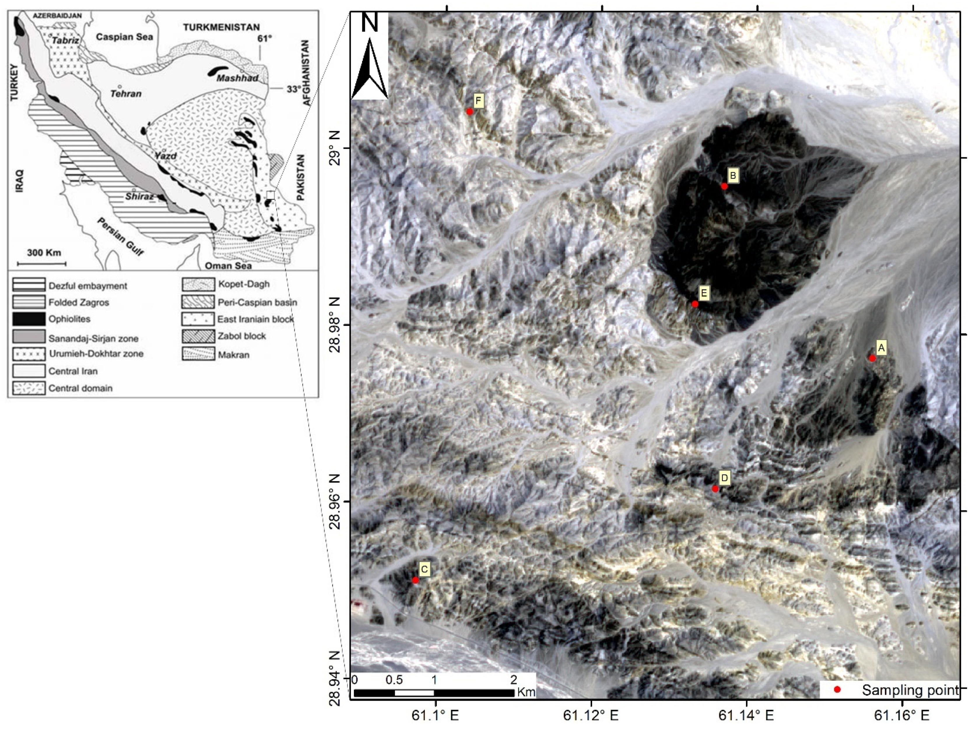
2. Geological Setting

The study area is located in the southeast of Iran and close to Mirjaveh, Sistan, and Baluchestan province, covering an area of about 66 square kilometers (Figure 1). Based on field observations and the study of thin sections, rock units mainly involve Quaternary and Oligocene igneous rocks and Eocene sedimentary rocks. Igneous rocks include dacite, andesite, and quartz monzonite, and Eocene sedimentary units include shale and sandstone [44]. The flysch units that date back to the Eocene cover most of the study area and mainly consist of shale and sandstone, and, in some areas, can be seen in a metamorphic form, such as slate and phyllite [44]. The sandstones are feldspar type and show a clastic (granular) texture. They are mostly affected by a poor degree of metamorphism, and slate somewhat expands with the growth of sericite crystals in relatively parallel directions. The major components of the sandstones are quartz and feldspar grains and a matrix consisting of clay minerals (kaolin) and calcite cement. Sericite minerals have also been added to this complex during the transformation. Dacite units in the study area are thick and consist of plagioclase, amphibole, biotite, and quartz, showing a porphyry texture. These units are coarse-grained and light in color. The dominant types of alteration in these rocks are argillic and sericitization. The Oligocene quartz monzonite units consist of plagioclase, alkali feldspar, and quartz minerals, showing a porphyry texture and light color. These units are scattered throughout the study area, particularly in the southeast region.
Major alteration types in the study area include argillic, sericitization, chloritization, silicic, propylitic, and iron oxide. The alteration zones are scattered throughout the study area and associated with igneous rocks. The predominant trends of faults are northwest–southeast (NW–SE) and northeast–southwest (NE–SW). The alteration zones mostly emerged due to the placement and formation of igneous units within the Eocene sedimentary units. Lead, zinc, manganese mineralization, and the association of pyrite with manganese-impregnated siliceous veins are observed in the margins of igneous units, and geochemical analyses confirm the gold anomaly. This type of mineralization corresponds to epithermal deposits based on field observations and sample analyses. In epithermal systems, metal precipitation from hot aqueous hydrothermal fluids can occur along lithological contacts. Planar discontinuities, such as sedimentary bedding, metamorphic foliations, planar igneous bodies, and unconformity surfaces, provide conduits for fluid flow and gold deposition [45]. In the study area, gold and other metals, such as manganese, lead, and zinc mineralizations, are found along the contacts of quartz monzonite and sedimentary units. It is noteworthy that younger alluvial units have covered quartz monzonite units in parts of the study area, and undercover exploration is required to identify potential mineralization.

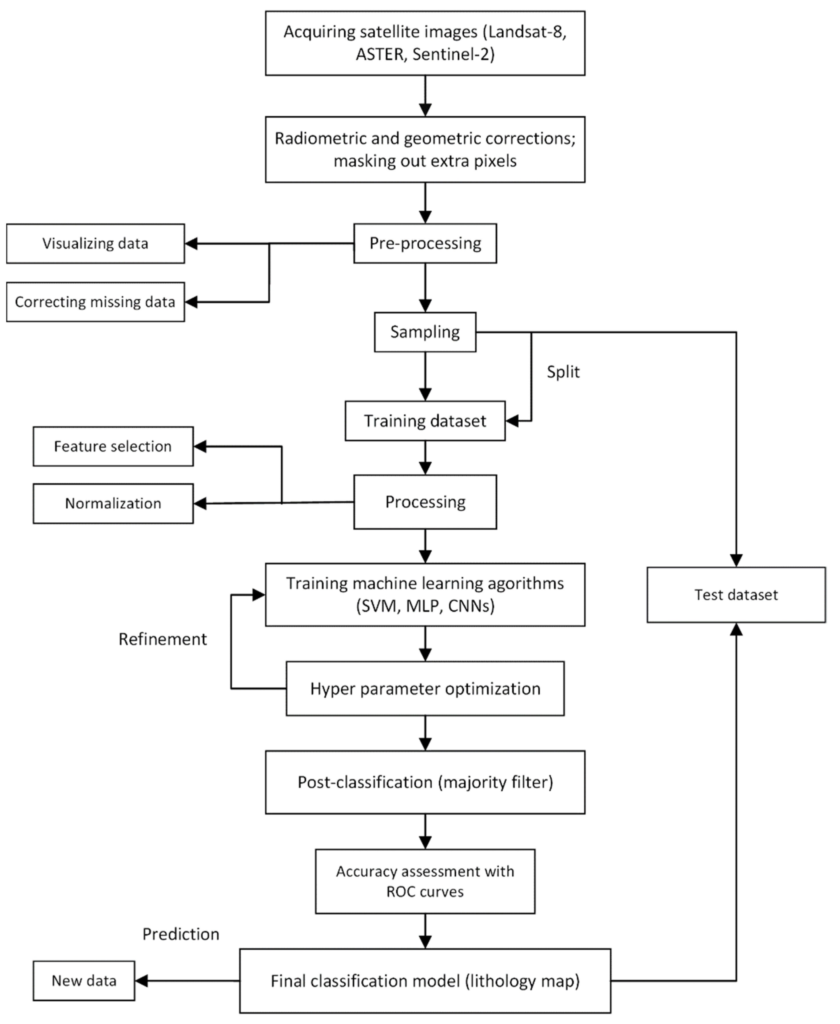
3. Materials and Methods

3.1. Remote-Sensing Data and Ground Truth

This study uses three different types of multispectral satellite images, including Landsat 8 OLI, ASTER, and Sentinel-2, for mapping lithological units. The technical performance and attributes of these data types are summarized in Table A1. Landsat 8 satellite was launched in 2013, carrying two sensors of OLI and thermal infrared sensor (TIRS) [46]. It provides images in 11 spectral bands with a spatial resolution ranging from 15 m (m) for a panchromatic band to 30 m in the visible and near-infrared (VNIR) and short-wave infrared (SWIR) ranges. The last two thermal bands, i.e., bands 10 and 11, have a resolution of 100 m [46]. ASTER sensor was launched on the Terra platform in 1999 [47], which significantly improved the capability of geological remote sensing for mapping purposes. ASTER has three VNIR bands with a spatial resolution of 15 m, six SWIR bands with a 30 m resolution, and five thermal infrared bands with a 90 m resolution [47]. The Sentinel-2 is a group of twin satellites in the same sun-synchronous orbit, phased at 180 degrees apart: Sentinel-2A and Sentinel-2B. The multispectral instrument onboard collects data in 13 spectral bands, ranging from VNIR to SWIR. The spatial resolution of this satellite is varied from 10 to 60 m [48]. In this study, we used those spectral bands that are of interest in geological remote sensing because they show characteristic behaviors, such as high absorption or reflectance in target lithological units. Accordingly, six bands of OLI (2, 3, 4, 5, 6, and 7), nine bands of ASTER (1, 2, 3, 4, 5, 6, 7, 8, and 9), and ten bands of Sentinel-2 (2, 3, 4, 5, 6, 7, 8, 8a, 11, and 12) are selected as the input data for mapping lithological units [7].
A cloud-free Landsat 8 scene covering the study area was acquired from the US geological survey Earth resources observation and science (EROS) center (earthexplorer.usgs.gov accessed on 20 November 2021). This level-1T (terrain corrected) image was captured on 4 June 2017. The ASTER scene used in this study was captured on 12 September 2003. It is a cloud-free level-1-precision terrain-corrected registered at-sensor radiance product (ASTER_L1T) obtained from the USGS EROS center. A cloud-free Sentinel-2A scene covering the study area was also acquired from the European space agency via the Copernicus open-access hub (scihub.copernicus.eu accessed on 20 November 2021) captured on 6 July 2017. The Sentinel-2 image used in this study is a level-1C top-of-atmosphere reflectance product, including radiometric and geometric corrections and orthorectification [48].
Ground truth refers to the information gathered on-site and represents mapped features and materials on the ground [49]. The ground-truth dataset consists of a set of images and labels, as well as an object-recognition model that involves the count, location, and relationships of key features. Depending on the location of the study area, labels are either specified by hand or automatically by image processing. Those features detected as ground-truth data are fed into a classifier at run-time to calculate the correspondence between identified and modeled features [50]. We used ground-truth data to train and test our models and create classified maps. Figure 2 represents a map showing the ground-truth dataset used in this study and consisting of nine rock types obtained by fieldwork.

3.2. Preprocessing

The satellite data used in this study were pre-georeferenced to the universal transverse Mercator (UTM) zone 40 North; hence, no geometric correction is needed. The Landsat 8 OLI and ASTER data are radiometrically corrected by the log-residual algorithm, available within the ENVI software package (l3harrisgeospatial.com/Software-Technology/ENVI, accessed on 20 November 2021), which reduces the noise from topography, instruments, and sun illumination. This method works with the visible and near-infrared to short-wave infrared (VNIR–SWIR) wavelength range and provides an atmospheric-corrected surface reflectance image of the study area. It is a quick solution for converting radiance-calibrated data to apparent reflectance. The SWIR bands of the ASTER data are resampled to the spatial resolution of the visible and near-infrared (VNIR) bands, i.e., 15 m, using the nearest neighbor technique, and a stacked data layer, using the VNIR plus the short-wave infrared (SWIR) bands, is created for further processing. The atmospheric correction is included by the Sentinel-2 data type used in this study. The VNIR + SWIR bands of the Sentinel-2 data are stacked by using the nearest neighbor technique, and a ten-band dataset with a spatial resolution of 10 m is generated. Prior to processing the remote-sensing data, they are all resized to a specific frame covering the target area.

3.3. Machine Learning Methods

ML methods are able to discover complex relationships in high-dimensional data [51]. For instance, these methods can automatically learn the relationship between reflectance spectra and target features in a study area, such as mineral occurrences. Machine-learning methods have been demonstrated to be robust against noise and uncertainties in spectral and ground-truth observations [52]. SVMs are supervised ML methods for classification and regression problems [53]. During training, SVM models create a hyperplane with the greatest maximum distances between data points in various groups, i.e., the largest margins [54]. Support vectors are the data points nearest to the hyperplane that specify the hyperplane’s orientation. The dimensions of the hyperplane decision boundary are determined by the number of input features that must be classified [55]. The SVM has greatly found its application in remote sensing, particularly in geological remote sensing for classifying geological features and targeting ore deposits [1,56,57,58]. Remote-sensing data usually involve groups that are not linearly separable, which becomes a challenge for conventional ML methods. In such instances, a nonlinear kernel function is used to transfer the data from the input feature space to a higher-dimensional feature space, spreading the data points so that they can be separated by a linear hyperplane [26]. A polynomial (homogeneous or heterogeneous) function, a Gaussian radial basis function, and a sigmoid (hyperbolic tangent) function, among others, are nonlinear kernels that are widely used in SVMs [26].
Neural networks are motivated by the learning process of biological neural systems and have been widely used to analyze remotely sensed data [7]. Over the past few decades, there has been tremendous progress in the area of neural networks; hence, canonical neural networks are known as simple neural networks, and larger and more complex architectures are known as deep neural networks or deep-learning methods [32,40]. The prominence of neural networks in remote-sensing data analysis is mainly due to their capacity to learn complex patterns while accounting for any complex nonlinear relationship in data [59]. Simple neural networks have demonstrated high efficiency in classifying geological features and discovering mineralization zones [20,54,60]. This study applies simple neural networks, also known as MLP, as a supervised learning algorithm to train our model, considering its capability to learn nonlinear relationships. MLP can learn a nonlinear function approximator for classification or regression, given a collection of features and objectives. It differs from logistic regression models since it can include one or more nonlinear layers, which are known as hidden layers between input and output layers [61].
CNNs are one of the different types of deep neural networks that feature the automatic extraction of features from image-based datasets [62]. CNNs caused advancements in image processing, target identification, and other disciplines [63]. CNNs have been widely utilized in image processing and have matured into a potent and ubiquitous deep learning model [64]. Recently, an improved CNN, with even fewer parameters, was introduced to solve problems such as overfitting and gradient vanishing [65]. Another study introduced a novel reconstruction technique based on CNNs with high speed and performance [66]. In terms of advancement in CNN approach, researchers [67] described the improvements made to the CNN in various aspects, such as layer design, activation function, loss function, regularization, optimization, and fast computation. CNNs use convolutional and pooling layers that enable automated feature extraction to draw out spatial information from image data. A typical CNN model consists of several pairs of convolutional and pooling layers, followed by a simple neural network of fully connected layers. We did not use pooling layers in our model architecture, since they aim to find objects. The convolution layer is made up of several feature maps that are generated by the convolution of the input image with a specific kernel. Each convolution kernel is a weight matrix, forming a two-dimensional representation of a single channel [62]. CNNs consider neighboring pixels and rely on the pattern and texture, not just one pixel at a time. In classifying a mid-resolution satellite image similar to those used in this study, the objective is to classify each pixel based on its digital number across different bands. We investigated the role of digital numbers of neighboring pixels in determining the class of each pixel. Each set of neighboring pixels fed into the CNN algorithm is called a chip, and they are created by setting two parameters, namely the size of the moving window and stride, as illustrated in Figure 3.

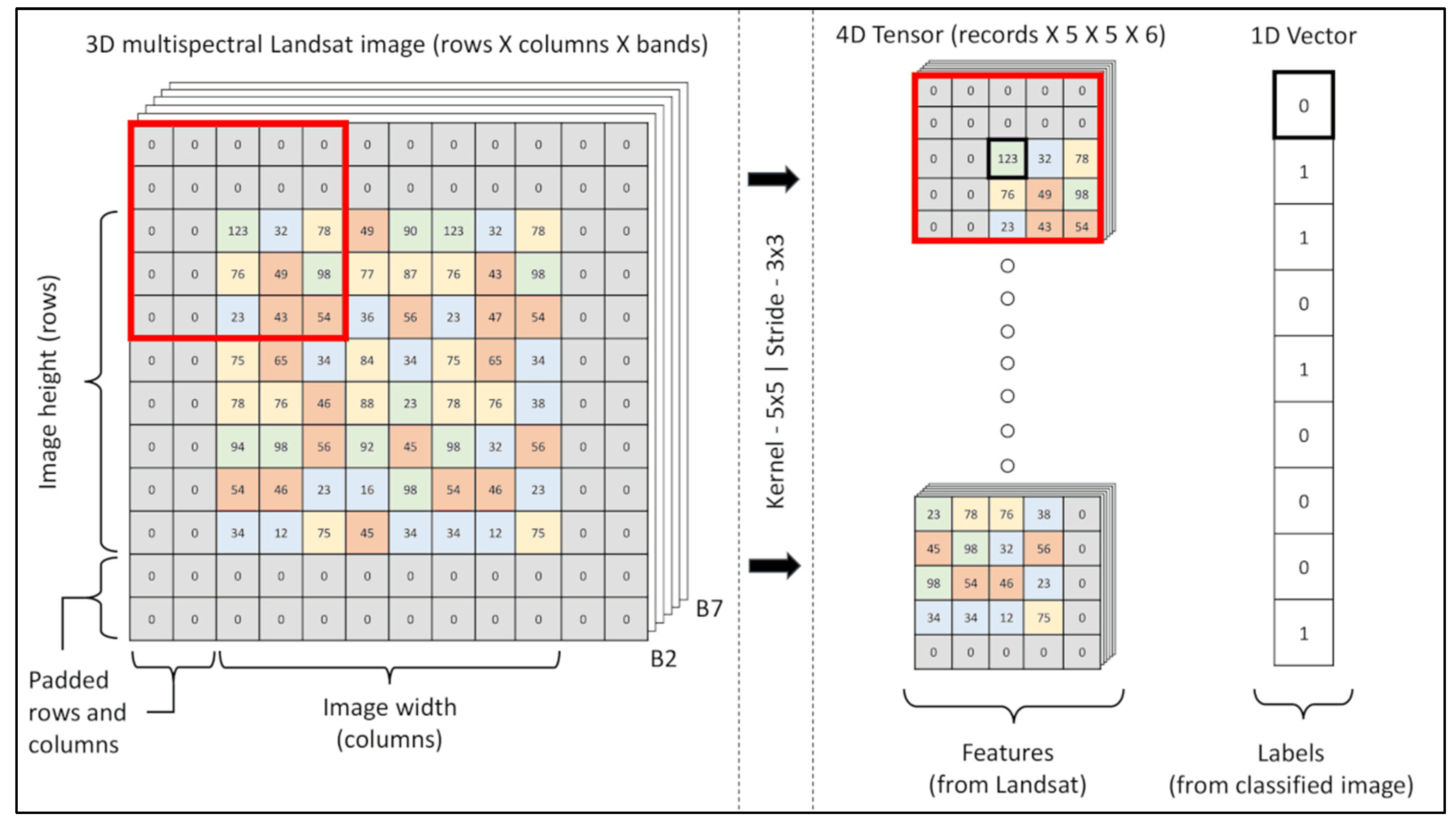
3.4. Framework and Experimental Setup

In Figure 4, we propose a framework in which SVMs, MLP, and CNNs are applied on three different types of multispectral remote-sensing data to investigate their efficiency in discriminating between lithological units. The initial steps involved loading and preprocessing remote-sensing and ground-truth datasets as inputs to our modeling process. We scaled the input datasets in the next step to ensure that all the features were treated equally. For instance, neural networks are sensitive to the input data distribution because they naturally tend to give more importance to features with higher values [68]. The data can either be scaled in the range of zero to one (normalized) or minus one to one (standardized). In this study, we used standardized data to train the SVM and MLP models and normalized data for the CNN model, although this cannot have a tangible effect on the modeling accuracy. We used the statistical properties of each of the input spectral bands for scaling them. The input data were split into two halves, i.e., training and test, to evaluate the performance of the model at a later stage. We define a function for this purpose and the train-test proportion considered is 75–25 percent.
The number of pixels along the x-axis and y-axis of the OLI, ASTER, and Sentinel-2 images is 257 × 289, 513 × 577, and 770 × 866, respectively. As mentioned earlier, each pixel in these images represents a square cell covering an area of 900, 225, and 100 square meters on the ground surface. Implementing each ML method and creating models requires setting a number of hyperparameters. This study experimented with different values to create each model and selected those providing the most accurate result. In the case of SVM, we used a radial basis function (RBF) kernel and a tolerance value of 0.001 with no limit for the number of iterations. In MLP, we used 15 hidden neurons and a maximum of 400 iterations (epochs), using Adam as a solver. Moreover, we used the rectified linear unit function (ReLU) as an activation function for the hidden layer and the Softmax activation for the output layer.
As shown in Figure 5, our CNN model uses two convolution layers with a kernel size of 7 × 7, stride of 7, and fully linked layers. These layers are a network of serially connected dense layers used for classification. In a fully connected network, every neuron from the first layer is connected to every neuron in the second layer. We examined other kernel sizes and strides, and the best accuracy was achieved by the mentioned values. Model architectures are sensitive, and the same model architecture cannot be expected to provide similar accuracy using different kernel sizes. Therefore, a few minor modifications in the architecture are expected. We used the ReLU activation function for the input layers and the Softmax activation function in the final layer for classification in the CNN model architecture. Furthermore, we used a root-mean-squared propagation optimizer with a maximum of 20 training epochs.
We used the majority analysis with a three-by-three kernel as a post-classification tool available within the ENVI software package in order to change spurious pixels within a large single class to that class. The center pixel in the kernel was replaced with the class value that a majority of the pixels in the kernel have [69]. The majority analysis required a given center pixel weight to generalize each classified map, and a neighborhood was built around each pixel identified by the user-defined distance. The number of pixels belonging to various groups within this neighborhood are counted, and the center pixel is assigned to the class that corresponds to the rest of the pixels in the neighborhood [69].
Along with this study, a Jupyter notebook based on the Python programming language was released that helps exploration geologists quickly implement the proposed framework. The link to this notebook is available in the supplementary materials section. It enables the user to rapidly map lithological units by using different types of remote-sensing data. A variety of packages have been used in this notebook, among which scikit-learn and TensorFlow packages are the most important. The scikit-learn package was used to create conventional models, i.e., SVM and MLP, and the TensorFlow package was applied to implement CNNs.

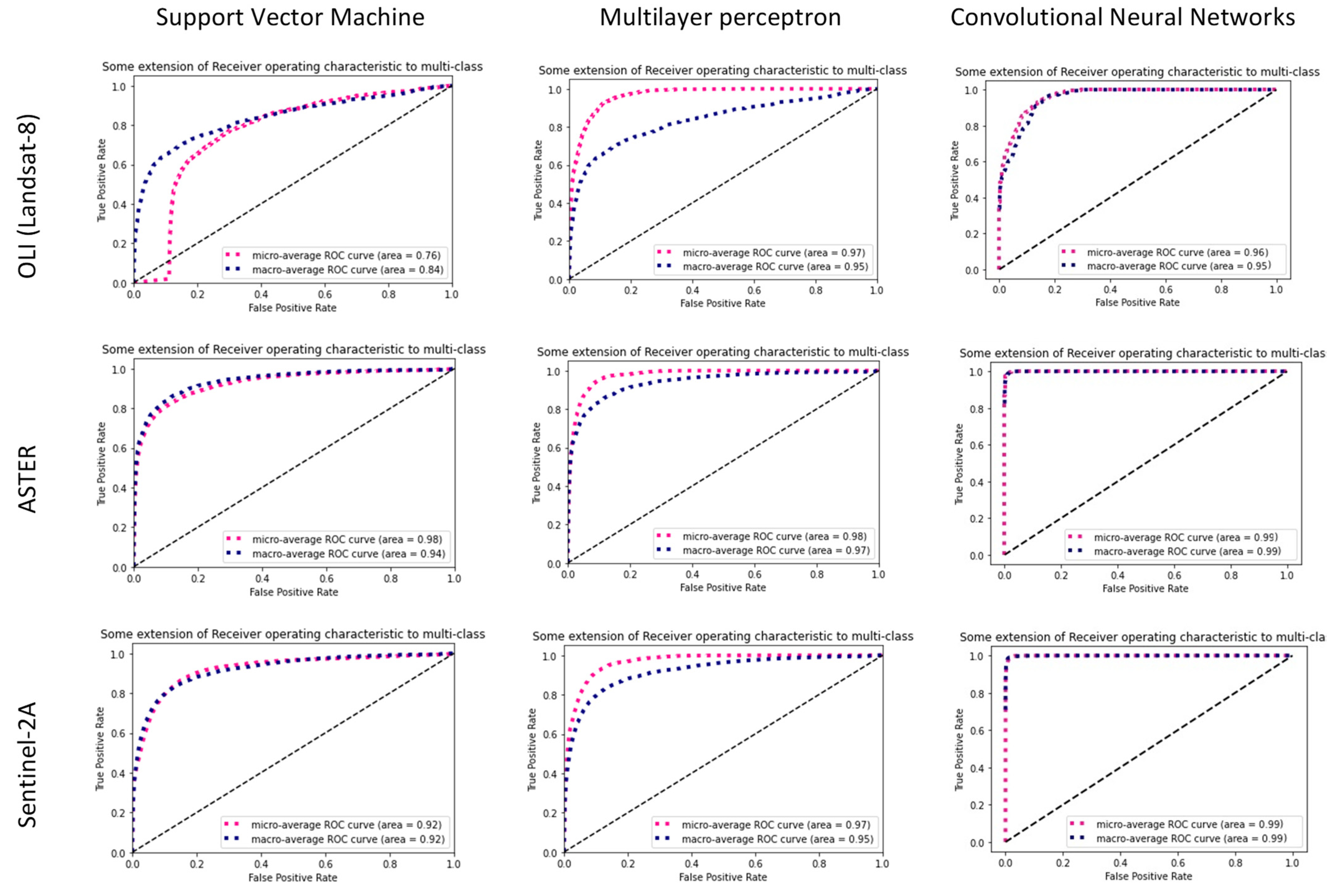
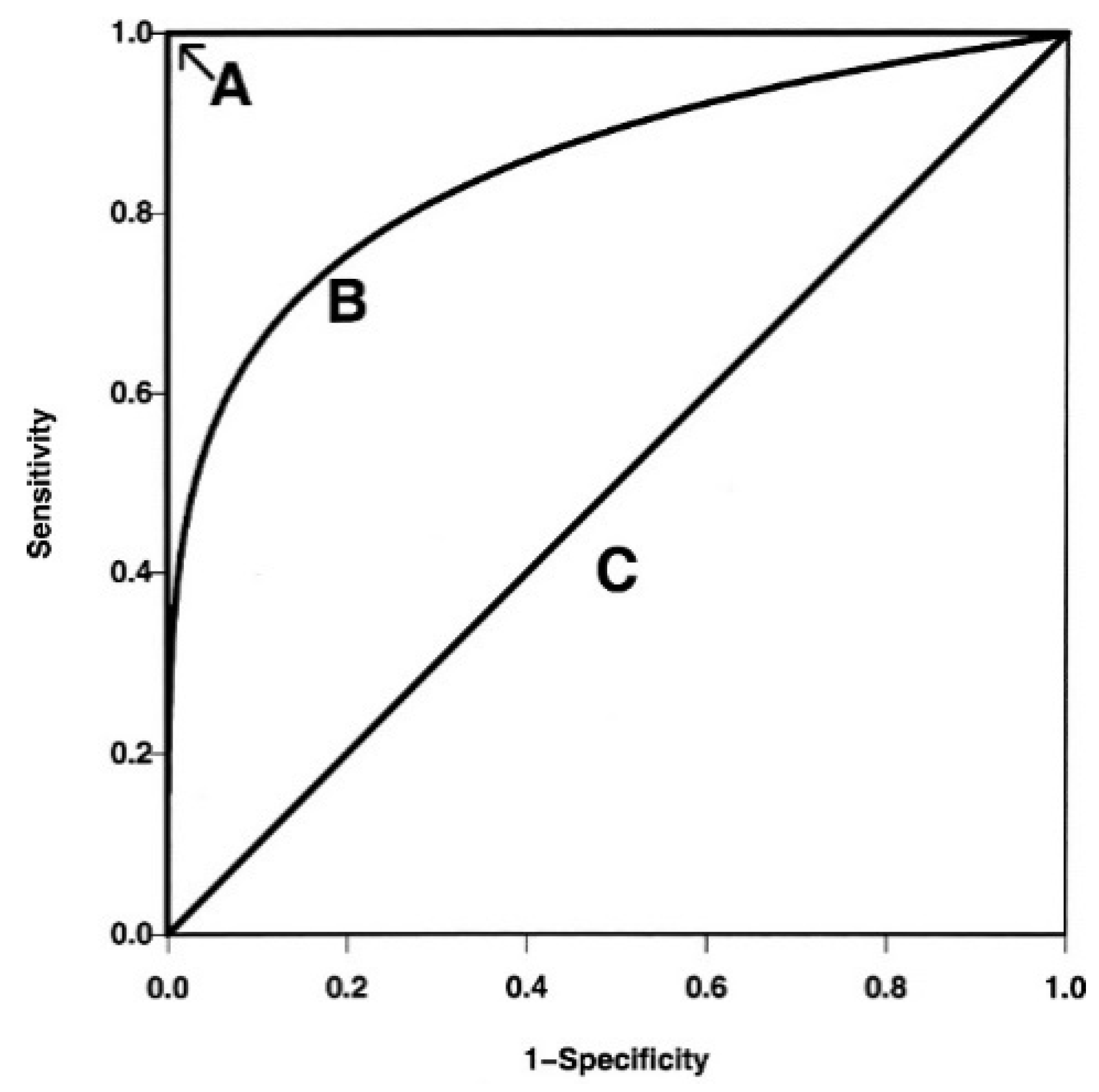
3.5. Receiver Operating Characteristics

The evaluation of model accuracy is a critical stage in every classification. In this study, receiver operating characteristics (ROCs) [70] were used to evaluate the classification accuracy of each output map. The ROC curves have a y-axis representing the true-positive (sensitivity) rate and an x-axis for false-positive rate (specificity), as shown in Figure A1. This means that the ideal point is in the top left corner of the chart, with a false-positive rate of zero and a true positive rate of one. This is far from true, but it does imply that a greater area under the curve (AUC) [70] is generally preferable. The ROC curve for random chance is the 45° diagonal line linking (0,0) and (1,1). The gold-standard ROC curve is the line joining (0, 0) to (0, 1) and (0, 1) to (1, 1). In general, ROC curves fall between these two extremes. The area under the ROC curve is a summary metric that averages diagnostic precision over a range of test values (Figure A1) [67].
The steepness of ROC curves is also significant, as it is optimal to maximize true-positive rate while also minimizing false-positive rates. In binary classification, ROC curves are commonly used to investigate the performance of a classifier. The performance must be binarized to apply the ROC curve and ROC area to multi-label classification. One ROC curve can be drawn for each class, but a ROC curve can also be drawn by treating each member of the label indicator matrix as a binary predictor (micro-averaging). Another assessment criterion for multi-label classification is macro-averaging, which assigns equal weight to each label’s classification [71].

4. Results

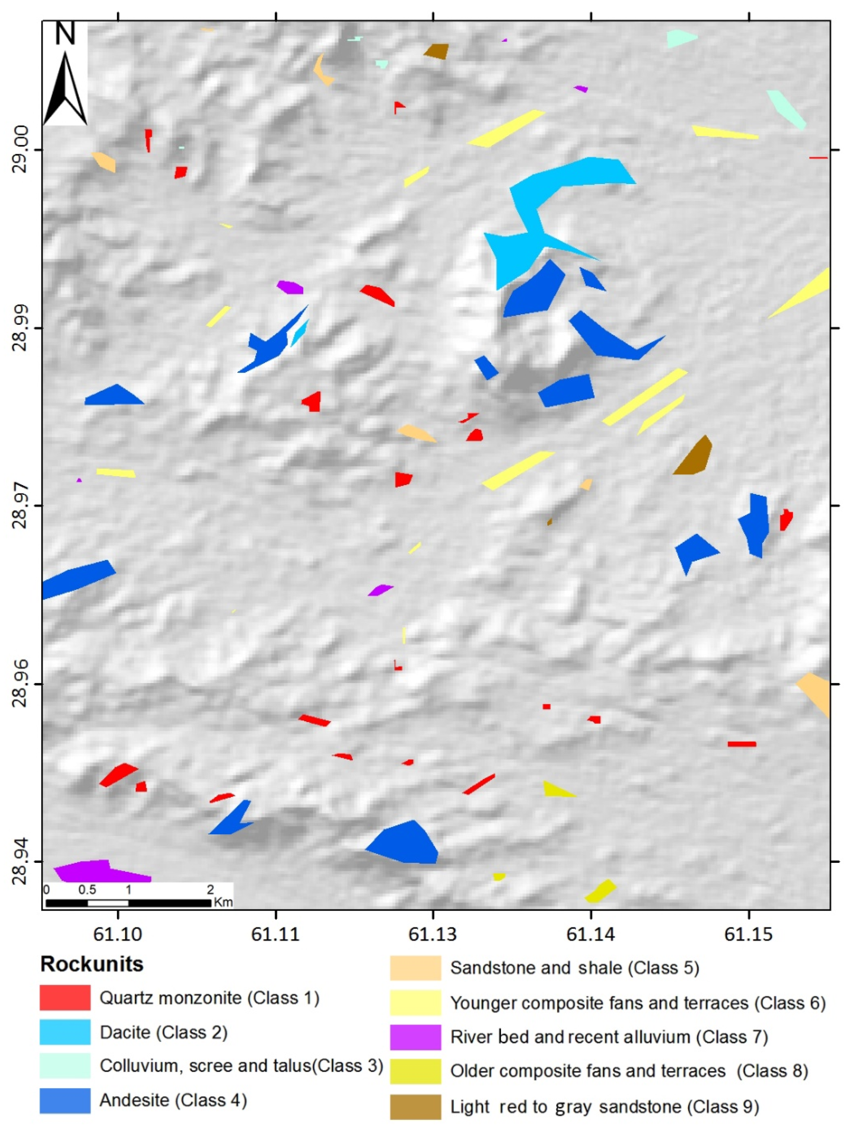
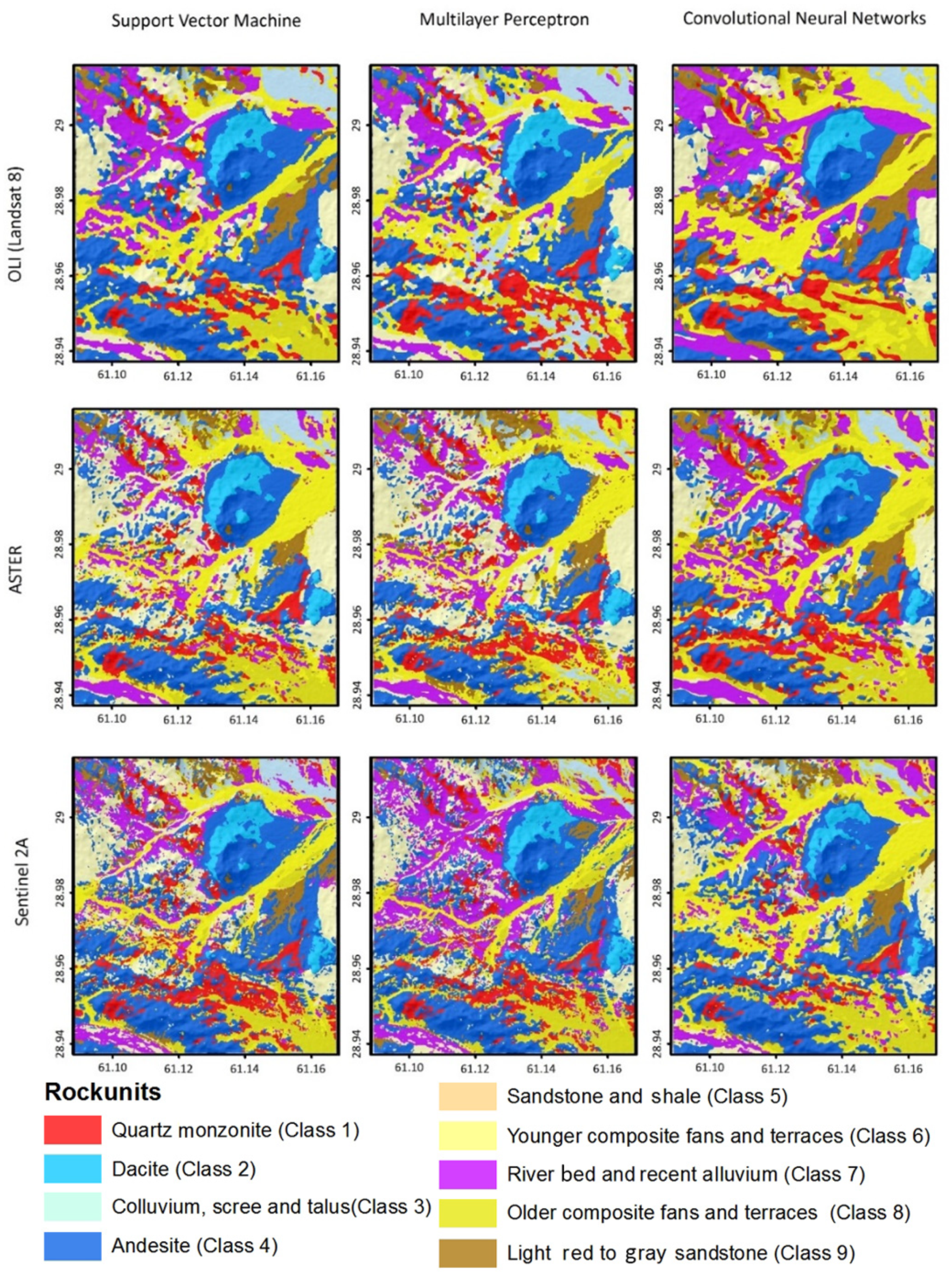
4.1. Classified Lithological Maps

The proposed framework was applied to the spectral subsets of three different types of remote-sensing data that were selected based on the spectral characteristics of target geological features in the study area, i.e., lithological units. Three lithological maps for each data type were created by applying different ML methods (SVM, MLP, and CNNs), as shown in Figure 6. Each class represents a specific lithological unit, and there are nine classes on each map (Figure 2). The spatial resolution of maps is different, and it is based on the spatial resolution of the input data and varies from 10 to 30 m.
According to the classified maps, most of the study area consists of Quaternary, Oligocene igneous, and Eocene sedimentary rocks. The flysch units that date back to Eocene cover most of the area and mainly consist of shale and sandstone (class 5), and they can be seen as a light red to gray sandstone (class 9) in some areas. Igneous rocks include dacite (class 2), andesite (class 4), and quartz monzonite (class 1), which are scattered throughout the study area, mainly striking northwest–southeast. Quaternary deposits cover the rock units in some places and include colluvium scree and talus (class 3), younger composite alluvial fans and terraces (class 6), older composite alluvial fans and terraces (class 8), and riverbed and recent alluvium (class 7).

4.2. Accuracy Assessment and Validation

Table 1 depicts the accuracy of each class, and Figure 7 demonstrates the micro and macro average ROC curve for all nine classified maps. According to the ROC curves shown in Figure 7, the lithological units were classified more accurately by using the combination of CNN and ASTER data. However, the result is almost the same as Sentinel-2 data. The AUC of micro and macro averages is close to one in these plots. Considering the AUCs, the MLP outperforms the SVM, and it is ranked second in terms of accuracy. On the other hand, after the ASTER data, the Sentinel-2 data yielded the most accurate results for lithological mapping in the study area, and the OLI is ranked last, which could be anticipated. The combination of SVM and OLI shows the lowest accuracy, where the micro average is 0.76, and the macro average is 0.84.
In addition to the ROC curves, several rock samples were collected from the study area to validate the lithological maps, particularly in places with little ground-truth data. These samples were mostly collected from the places where rock types are classified as quartz monzonite, andesite, dacite, and sandstone, and three of them, along with their polished thin sections, are shown in Figure 8. The sampling locations are shown in Figure 1 and labeled as A–C. The results obtained by investigating the polished thin sections indicate that the classifiers have been successful in the sampling regions. Moreover, we analyzed three samples from the study area, as shown in Figure 1, labeled as D–F, using the inductively coupled plasma–mass spectrometry (ICP–MS) for determining the concentration values of gold, manganese, lead, and zinc. Based on the laboratory analysis, the margins of igneous units in the study area are of great importance in terms of economic mineralization, and the geochemical analyses confirm this observation (Table 2).

5. Discussion

Based on the prediction accuracy obtained by the ROC curves and the thin-section analysis of the rock samples collected from the study area, the combination of CNN and ASTER data provided the most accurate lithological map for our study area. Although the Sentinel-2 data provide a better spatial resolution in the VNIR bands, i.e., 10 m, and the number of bands in this range are more than the ASTER data, this data type was less successful in terms of classifying lithological units compared to the ASTER data; however, the contrast is insignificant. The ASTER data proved to be an efficient data type for alteration mapping [12,24] and, based on the results of this study, for lithological mapping. It is noteworthy that the results can probably be different in other regions depending on the extent and geological characteristics of the target area, such as dominant rocks and minerals and the spectral characteristics of the features to be mapped. The SWIR bands of ASTER data have great advantages for lithological mapping [72], particularly in an area with altered rock types, since they mostly show unique spectral behaviors in this range. However, even our most accurate computer-generated lithological map displays some inconsistencies compared to field observations. For example, sandstones are mapped inside dacite and andesite units in some areas, or andesite units are seen within quartz monzonite units. These issues might be addressed by collecting more training data or improving the classified maps through checking suspicious areas.
The SVM and MLP methods performed well in mapping lithological units in the study area and provided valuable information regarding the lithological units. However, CNNs were more successful in providing an accurate lithological map. Apart from computationally efficient characteristics of CNNs, we also had less noisy pixels in our classified maps by CNNs because of considering neighboring pixels in modeling and relying on the pattern and texture, not just one pixel at a time. The extremely high accuracy of the model we achieved by combining the CNNs and ASTER data can be considered as a consequence of the low number of mixed pixels in our testing set. A lower accuracy would likely be achieved in regions with a more complicated geological setting and mixed pixels. The model performed well in predicting test classes, because the classes were easily differentiable in the multidimensional space. Therefore, the model learned well how to distinguish between classes for pure pixels.
In MLP classifiers, the tested datasets require more hidden units, and the complexity is managed by holding the number of these units small, while the SVM complexity is independent of the dimension of the datasets. SVMs are based on structural risk minimization, while MLP classifiers implement empirical risk minimization. Another difference is the complexity of the network. MLP networks that implement global approximation strategies typically use very few hidden neurons. On the other hand, SVMs are based on a local approximation strategy and use a large number of hidden units [73]. However, the MLP network was generally more accurate than SVM for lithological classification using remote-sensing data in this research. CNNs also involve some disadvantages; for example, CNNs do not encode the position and orientation of objects, they lack the ability to be spatially invariant to the input data, and a large amount of training data is needed. However, CNNs with the hyperparameters used in this study were the most successful method.
The map provided by the proposed framework can be considered as an initial lithological base map. This map can be improved by carrying out comprehensive fieldwork with predefined profiles and a reasonable spacing, along with collecting a required number of samples. The resultant map of this process can be worth interpreting and deciding whether to continue the exploration operation in a region. According to the laboratory analysis and field observations, gold, manganese, lead, and zinc mineralizations and the interaction of pyrite with manganese-impregnated siliceous veins have been found in the margins of igneous units and mapped accurately in the lithological maps. In addition, the geochemical analysis of the samples collected from potential locations supports the high probability of economic gold mineralization in the study area.
ML methods have been widely used in remote-sensing-data analysis, but there are still gaps in predictive uncertainty quantification. In general, it is difficult to assess the uncertainty of remote-sensing model applications. Model validation is usually performed by comparing it with ground truth or alternative information believed to represent ground truth. Different approaches have been developed to address validation issues, and different models are possible. Bayesian inference provides a principled approach for quantifying the uncertainty of model parameters. Recently, there have been major advances in Bayesian neural networks and Bayesian deep learning. However, these methods have not been much used for remote sensing, and their application for geological exploration is absent. In future studies, we are planning to use other deep learning methods to map geological features [34], such as Bayesian neural networks, since it provides principled uncertainty quantification via the posterior distribution [74]. These methods may provide a meaningful interpretation of remote-sensing data in the face of challenges, such as data noise, sparse datasets, and missing data. Uncertainty quantification using Bayesian inference can be used to predict the uncertainty associated with model parameters and data. As a result, applying these methods can play an essential role in the evolution of geological remote sensing and improve its efficiency in mineral exploration.

6. Conclusions

Nowadays, geoscientists are equipped with the latest groundbreaking and efficient ML methods to work with big data, such as remote-sensing data. In this study, three different ML methods were used to process three types of remote-sensing data by mapping lithological units of a region in the southeast of Iran. We classified the remote-sensing data and discriminated lithological units, providing valuable information for mineral exploration. We showed the efficiency of applying machine- and deep-learning techniques on remote-sensing data and observed that the CNN and ASTER data combination provides the most accurate lithological map of the study area based on the ROC curves, and the test data were successfully predicted. Such maps can be considered base maps for further geological fieldworks and a reliable factor aiding in deciding for mineral-exploration operations.
We addressed the challenges of mapping lithological units on the ground and proposed a framework to overcome them. Our framework presented in a Jupyter notebook is an open-source community tool for mapping lithological units by using multi- or hyperspectral data. This notebook can significantly enhance the ability of exploration geologists to map lithological units. It can be considered a fast, reliable, and low-cost approach for generating a remote-sensing evidential layer and delineating favorable loci for precious mineral deposits at any stage of an exploration program. The framework can be improved by optimizing SVM, MLP, and CNN hyperparameters. Moreover, other ML methods, such as random forest, naive Bayes, k-nearest neighbors, and minimum distance, can be added to this framework to compare their efficiency with other methods.

Supplementary Materials

The Jupyter notebook and datasets used in this study are available at https://github.com/sydney-machine-learning/deeplearning_lithology (accessed on 20 November 2021).

Author Contributions

H.S. and E.F. made an equal contribution to this study. Conceptualization, H.S., E.F. and R.C.; methodology, H.S., E.F. and R.C.; software, H.S., E.F. and R.C.; validation, H.S. and E.F.; writing—original draft preparation, H.S., E.F., E.H. and R.C.; writing—review and editing, A.B.P., B.P. and D.M.; visualization, H.S. and E.F.; supervision, R.C. All authors have read and agreed to the published version of the manuscript.

Funding

This research was supported by the Australian Research Council (Grant No.: LP210100173).

Data Availability Statement

The datasets used in this study, including remote sensing and ground truth data, are available at https://github.com/sydney-machine-learning/deeplearning_lithology (accessed on 20 November 2021).

Acknowledgments

The authors would like to thank L. S. Galvao for handling this paper and anonymous reviewers for providing constructive comments that improved the manuscript.

Conflicts of Interest

The authors declare no conflict of interest.

Appendix A

Table A1. Technical performance and attributes of Landsat 8, Sentinel-2, and ASTER data [46,47,48].
Satellite/SensorSubsystemBand NumberSpectral Range (Micrometers)Ground Resolution (m)Swath Width (Km)Year of Launch
Landsat 8OLIBand 1 Coastal Aerosol0.43–0.45301852013
Band 2 Blue0.45–0.5130
Band 3 Green0.53–0.5930
Band 4 Red0.64–0.6730
Band 5 Near Infrared (NIR)0.85–0.8830
Band 6 SWIR 11.57–1.6530
Band 7 SWIR 22.11–2.2930
Band 8 Panchromatic0.50–0.6815
Band 9 Cirrus1.36–1.3830
TIRBand 10 Thermal Infrared (TIRS 1)10.60–11.19100
Band 11 Thermal Infrared (TIRS 2)11.50–12.51100
ASTERVNIRBand 10.520–0.60015601999
Band 20.630–0.69015
Band 30.780–0.86015
SWIRBand 41.600–1.70030
Band 52.145–2.18530
Band 62.185–2.22530
Band 72.235–2.28530
Band 82.295–2.36530
Band 92.360–2.43030
TIRBand 108.125–8.47590
Band 118.475–8.82590
Band 128.925–9.275
Band 1310.250–10.950
Band 1410.950–11.650
Sentinel-2Band 1 Coastal Aerosol0.433–0.453602902015
Band 2 Blue0.458–0.52310
Band 3 Green0.543–0.57810
Band 4 Red0.650–0.68010
Band 5 Red Edge 10.698–0.71320
Band 6 Red Edge 20.733–0.74820
Band 7 Red Edge 30.773–0.79320
Band 8 NIR0.785–0.90010
Band 8A Narrow NIR0.855–0.87520
Band 9 Water-Vapor0.935–0.95560
Band 10 SWIR/Cirrus1.360–1.39060
Band 11 SWIR 11.565–1.65520
Band 12 SWIR 22.100–2.28020
Figure A1. Three imaginary ROC curves reflecting the gold standard’s diagnostic precision (lines A; AUC = 1) on the upper and left axes in the unit square, a normal ROC curve (curve B; AUC = 0.85), and a diagonal line leading to random chance (line C; AUC = 0.5) are shown. The ROC curve shifts toward A as the diagnostic-test precision increases and the AUC reaches 1 [75].
Remotesensing 14 00819 g0a1

References

  1. Othman, A.; Gloaguen, R. Improving lithological mapping by SVM classification of spectral and morphological features: The discovery of a new chromite body in the Mawat ophiolite complex (Kurdistan, NE Iraq). Remote Sens. 2014, 6, 6867–6896. [Google Scholar] [CrossRef] [Green Version]
  2. Qing, F.; Zhao, Y.; Meng, X.; Su, X.; Qi, T.; Yue, D. Application of machine learning to debris flow susceptibility mapping along the China–Pakistan Karakoram highway. Remote Sens. 2020, 12, 2933. [Google Scholar] [CrossRef]
  3. Torabi, A.; Berg, S.S. Scaling of fault attributes: A review. Mar. Pet. Geol. 2011, 28, 1444–1460. [Google Scholar] [CrossRef]
  4. Ding, W.-C.; Li, T.-D.; Chen, X.-H.; Chen, J.-P.; Xu, S.-L.; Zhang, Y.-P.; Li, B.; Yang, Q. Intra-continental deformation and tectonic evolution of the West Junggar Orogenic Belt, Central Asia: Evidence from remote sensing and structural geological analyses. Geosci. Front. 2020, 11, 651–663. [Google Scholar] [CrossRef]
  5. Liu, L.; Zhou, J.; Jiang, D.; Zhuang, D.; Mansaray, L.R.; Zhang, B. Targeting mineral resources with remote sensing and field data in the Xiemisitai area, West Junggar, Xinjiang, China. Remote Sens. 2013, 5, 3156–3171. [Google Scholar] [CrossRef] [Green Version]
  6. Radford, D.D.G.; Cracknell, M.J.; Roach, M.J.; Cumming, G. V Geological mapping in Western Tasmania using radar and random forests. IEEE J. Sel. Top. Appl. Earth Obs. Remote Sens. 2018, 11, 3075–3087. [Google Scholar] [CrossRef]
  7. Shirmard, H.; Farahbakhsh, E.; Müller, R.D.; Chandra, R. A review of machine learning in processing remote sensing data for mineral exploration. Remote Sens. Environ. 2022, 268, 112750. [Google Scholar] [CrossRef]
  8. Brimhall, G.H.; Dilles, J.H.; Proffett, J.M. The Role of Geologic Mapping in Mineral Exploration. Wealth Creat. Miner. Ind. Integr. Sci. Business Educ. 2005, 12, 221–241. [Google Scholar]
  9. Rowan, L.C.; Schmidt, R.G.; Mars, J.C. Distribution of hydrothermally altered rocks in the Reko Diq, Pakistan mineralized area based on spectral analysis of ASTER data. Remote Sens. Environ. 2006, 104, 74–87. [Google Scholar] [CrossRef]
  10. Latifovic, R.; Pouliot, D.; Campbell, J. Assessment of convolution neural networks for surficial geology mapping in the South Rae geological region, Northwest Territories, Canada. Remote Sens. 2018, 10, 307. [Google Scholar] [CrossRef] [Green Version]
  11. Asadzadeh, S.; de Souza Filho, C.R. A review on spectral processing methods for geological remote sensing. Int. J. Appl. Earth Obs. Geoinf. 2016, 47, 69–90. [Google Scholar] [CrossRef]
  12. Rezaei, A.; Hassani, H.; Moarefvand, P.; Golmohammadi, A. Lithological mapping in Sangan region in Northeast Iran using ASTER satellite data and image processing methods. Geol. Ecol. Landsc. 2020, 4, 59–70. [Google Scholar] [CrossRef] [Green Version]
  13. Lazecký, M.; Spaans, K.; González, P.J.; Maghsoudi, Y.; Morishita, Y.; Albino, F.; Elliott, J.; Greenall, N.; Hatton, E.; Hooper, A.; et al. LiCSAR: An automatic InSAR tool for measuring and monitoring tectonic and volcanic activity. Remote Sens. 2020, 12, 2430. [Google Scholar] [CrossRef]
  14. Beiranvand Pour, A.; Hashim, M. ASTER, ALI and Hyperion sensors data for lithological mapping and ore minerals exploration. Springerplus 2014, 3, 130. [Google Scholar] [CrossRef] [PubMed] [Green Version]
  15. Shirmard, H.; Farahbakhsh, E.; Beiranvand Pour, A.; Muslim, A.M.; Müller, R.D.; Chandra, R. Integration of selective dimensionality reduction techniques for mineral exploration using ASTER satellite data. Remote Sens. 2020, 12, 1261. [Google Scholar] [CrossRef] [Green Version]
  16. van der Meer, F.D.; van der Werff, H.M.A.; van Ruitenbeek, F.J.A.; Hecker, C.A.; Bakker, W.H.; Noomen, M.F.; van der Meijde, M.; Carranza, E.J.M.; de Smeth, J.B.; Woldai, T. Multi- and hyperspectral geologic remote sensing: A review. Int. J. Appl. Earth Obs. Geoinf. 2012, 14, 112–128. [Google Scholar] [CrossRef]
  17. Kuhn, S.; Cracknell, M.J.; Reading, A.M. Lithologic mapping using Random Forests applied to geophysical and remote-sensing data: A demonstration study from the Eastern Goldfields of Australia. Geophysics 2018, 83, B183–B193. [Google Scholar] [CrossRef]
  18. Farahbakhsh, E.; Chandra, R.; Olierook, H.; Scalzo, R.; Clark, C.; Reddy, S.; Müller, D. Computer vision-based framework for extracting tectonic lineaments from optical remote sensing data. Int. J. Remote Sens. 2020, 41, 1760–1787. [Google Scholar] [CrossRef]
  19. Sun, T.; Chen, F.; Zhong, L.; Liu, W.; Wang, Y. GIS-based mineral prospectivity mapping using machine learning methods: A case study from Tongling ore district, eastern China. Ore Geol. Rev. 2019, 109, 26–49. [Google Scholar] [CrossRef]
  20. Cracknell, M.J.; Reading, A.M. Geological mapping using remote sensing data: A comparison of five machine learning algorithms, their response to variations in the spatial distribution of training data and the use of explicit spatial information. Comput. Geosci. 2014, 63, 22–33. [Google Scholar] [CrossRef] [Green Version]
  21. Kanevski, M. Machine Learning for Spatial Environmental Data; EPFL Press: New York, NY, USA, 2009. [Google Scholar]
  22. Ye, B.; Tian, S.; Ge, J.; Sun, Y. Assessment of WorldView-3 data for lithological mapping. Remote Sens. 2017, 9, 1132. [Google Scholar] [CrossRef]
  23. Farahbakhsh, E.; Shirmard, H.; Bahroudi, A.; Eslamkish, T. Fusing ASTER and QuickBird-2 satellite data for detailed investigation of porphyry copper deposits using PCA; Case study of Naysian deposit, Iran. J. Indian Soc. Remote Sens. 2016, 44, 525–537. [Google Scholar] [CrossRef]
  24. Beiranvand Pour, A.; Hashim, M.; Hong, J.K.; Park, Y. Lithological and alteration mineral mapping in poorly exposed lithologies using Landsat-8 and ASTER satellite data: North-eastern Graham Land, Antarctic Peninsula. Ore Geol. Rev. 2019, 108, 112–133. [Google Scholar] [CrossRef]
  25. Sekandari, M.; Masoumi, I.; Beiranvand Pour, A.; Muslim, A.M.; Rahmani, O.; Hashim, M.; Zoheir, B.; Pradhan, B.; Misra, A.; Aminpour, S.M. Application of Landsat-8, Sentinel-2, ASTER and WorldView-3 spectral imagery for exploration of carbonate-hosted Pb-Zn deposits in the Central Iranian Terrane (CIT). Remote Sens. 2020, 12, 1239. [Google Scholar] [CrossRef] [Green Version]
  26. Yu, L.; Porwal, A.; Holden, E.-J.; Dentith, M.C. Towards automatic lithological classification from remote sensing data using support vector machines. Comput. Geosci. 2012, 45, 229–239. [Google Scholar] [CrossRef]
  27. Bressan, T.S.; Kehl de Souza, M.; Girelli, T.J.; Junior, F.C. Evaluation of machine learning methods for lithology classification using geophysical data. Comput. Geosci. 2020, 139, 104475. [Google Scholar] [CrossRef]
  28. Bachri, I.; Hakdaoui, M.; Raji, M.; Teodoro, A.C.; Benbouziane, A. Machine learning algorithms for automatic lithological mapping using remote sensing data: A case study from Souk Arbaa Sahel, Sidi Ifni Inlier, Western Anti-Atlas, Morocco. ISPRS Int. J. Geo-Inf. 2019, 8, 248. [Google Scholar] [CrossRef] [Green Version]
  29. Atangana Otele, C.G.; Onabid, M.A.; Assembe, P.S.; Nkenlifack, M. Updated lithological map in the Forest zone of the Centre, South and East regions of Cameroon using multilayer perceptron neural network and Landsat images. J. Geosci. Environ. Prot. 2021, 9, 120–134. [Google Scholar] [CrossRef]
  30. Venkatesh, Y.V.; Kumar Raja, S. On the classification of multispectral satellite images using the multilayer perceptron. Pattern Recognit. 2003, 36, 2161–2175. [Google Scholar] [CrossRef]
  31. Sergi, R.; Solaiman, B.; Mouchot, M.-C.; Pasquariello, G.; Pósa, P. Landsat-TM image classification using principal components analysis and neural networks. In Proceedings of the International Geoscience and Remote Sensing Symposium: Quantitative Remote Sensing for Science and Applications, Firenze, Italy, 10–14 July 1995; Volume 3, pp. 1927–1929. [Google Scholar]
  32. Neupane, B.; Horanont, T.; Aryal, J. Deep learning-based semantic segmentation of urban features in satellite images: A review and meta-analysis. Remote Sens. 2021, 13, 808. [Google Scholar] [CrossRef]
  33. He, Z.; Liu, H.; Wang, Y.; Hu, J. Generative adversarial networks-based semi-supervised learning for hyperspectral image classification. Remote Sens. 2017, 9, 1042. [Google Scholar] [CrossRef] [Green Version]
  34. Sang, X.; Xue, L.; Ran, X.; Li, X.; Liu, J.; Liu, Z. Intelligent high-resolution geological mapping based on SLIC-CNN. ISPRS Int. J. Geo-Inf. 2020, 9, 99. [Google Scholar] [CrossRef] [Green Version]
  35. Chen, Y.-Y.; Lin, Y.-H.; Kung, C.-C.; Chung, M.-H.; Yen, I.-H. Design and implementation of cloud analytics-assisted smart power meters considering advanced artificial intelligence as edge analytics in demand-side management for smart homes. Sensors 2019, 19, 2047. [Google Scholar] [CrossRef] [PubMed] [Green Version]
  36. Georgiou, T.; Liu, Y.; Chen, W.; Lew, M. A survey of traditional and deep learning-based feature descriptors for high dimensional data in computer vision. Int. J. Multimed. Inf. Retr. 2020, 9, 135–170. [Google Scholar] [CrossRef] [Green Version]
  37. Shambhu, S.; Koundal, D.; Das, P.; Sharma, C. Binary classification of COVID-19 CT images using CNN: COVID diagnosis using CT. Int. J. E-Health Med. Commun. 2022, 13, 1–13. [Google Scholar] [CrossRef]
  38. Yang, M.; Liu, Y.; You, Z. The Euclidean embedding learning based on convolutional neural network for stereo matching. Neurocomputing 2017, 267, 195–200. [Google Scholar] [CrossRef]
  39. Jing, L.; Zhao, M.; Li, P.; Xu, X. A convolutional neural network based feature learning and fault diagnosis method for the condition monitoring of gearbox. Measurement 2017, 111, 1–10. [Google Scholar] [CrossRef]
  40. Ma, L.; Liu, Y.; Zhang, X.; Ye, Y.; Yin, G.; Johnson, B.A. Deep learning in remote sensing applications: A meta-analysis and review. ISPRS J. Photogramm. Remote Sens. 2019, 152, 166–177. [Google Scholar] [CrossRef]
  41. Saliu, O.; Curilla, D.; Lennon, M.; Chung, A. Lessons learned: Deep learning for mineral exploration. In Proceedings of the First EAGE Conference on Machine Learning in Americas, Online, 22–24 September 2020. [Google Scholar]
  42. Mei, S.; Geng, Y.; Hou, J.; Du, Q. Learning hyperspectral images from RGB images via a coarse-to-fine CNN. Sci. China Inf. Sci. 2022, 65, 152102. [Google Scholar] [CrossRef]
  43. Litjens, G.; Kooi, T.; Bejnordi, B.E.; Setio, A.A.A.; Ciompi, F.; Ghafoorian, M.; van der Laak, J.A.W.M.; van Ginneken, B.; Sánchez, C.I. A survey on deep learning in medical image analysis. Med. Image Anal. 2017, 42, 60–88. [Google Scholar] [CrossRef] [Green Version]
  44. Parsolang Engineering Consultant Company. Map Report: Deh Reza Exploration Area, Sistan and Baluchestan Province; Parsolang Engineering Consultant Company: Tehran, Iran, 2021. [Google Scholar]
  45. Groves, D.I.; Santosh, M.; Zhang, L. A scale-integrated exploration model for orogenic gold deposits based on a mineral system approach. Geosci. Front. 2020, 11, 719–738. [Google Scholar] [CrossRef]
  46. Vaughn, I. Landsat 8 (L8) Data Users Handbook; US Geological Survey: Sioux Falls, SD, USA, 2019.
  47. Abrams, M.; Hook, S.; Ramachandran, B. ASTER User Handbook; Jet Propulsion Laboratory: Pasadena, CA, USA, 2002.
  48. SUHET. Sentinel-2 User Handbook; European Space Agency: Paris, France, 2015. [Google Scholar]
  49. Grosse, R.; Johnson, M.K.; Adelson, E.H.; Freeman, W.T. Ground truth dataset and baseline evaluations for intrinsic image algorithms. In Proceedings of the IEEE 12th International Conference on Computer Vision, Kyoto, Japan, 29 September–2 October 2009; pp. 2335–2342. [Google Scholar]
  50. Krig, S. Ground Truth Data, Content, Metrics, and Analysis. In Computer Vision Metrics; Springer: Berlin/Heidelberg, Germany, 2014; pp. 283–311. [Google Scholar]
  51. Maxwell, A.E.; Warner, T.A.; Fang, F. Implementation of machine-learning classification in remote sensing: An applied review. Int. J. Remote Sens. 2018, 39, 2784–2817. [Google Scholar] [CrossRef] [Green Version]
  52. Gewali, U.B.; Monteiro, S.T.; Saber, E. Machine learning based hyperspectral image analysis: A survey. arXiv 2018, arXiv:1802.08701. [Google Scholar]
  53. Liu, P.; Choo, K.-K.R.; Wang, L.; Huang, F. SVM or deep learning? A comparative study on remote sensing image classification. Soft Comput. 2017, 21, 7053–7065. [Google Scholar] [CrossRef]
  54. Maepa, F.; Smith, R.S.; Tessema, A. Support vector machine and artificial neural network modelling of orogenic gold prospectivity mapping in the Swayze greenstone belt, Ontario, Canada. Ore Geol. Rev. 2021, 130, 103968. [Google Scholar] [CrossRef]
  55. Abedi, M.; Norouzi, G.-H.; Bahroudi, A. Support vector machine for multi-classification of mineral prospectivity areas. Comput. Geosci. 2012, 46, 272–283. [Google Scholar] [CrossRef]
  56. Pal, M.; Rasmussen, T.; Porwal, A. Optimized lithological mapping from multispectral and hyperspectral remote sensing images using fused multi-classifiers. Remote Sens. 2020, 12, 177. [Google Scholar] [CrossRef] [Green Version]
  57. Abdolmaleki, M.; Rasmussen, T.M.; Pal, M.K. Exploration of IOCG mineralizations using integration of space-borne remote sensing data with airborne geophysical data. ISPRSn Int. Arch. Photogramm. Remote Sens. Spat. Inf. Sci. 2020, XLIII-B3-2, 9–16. [Google Scholar] [CrossRef]
  58. Cardoso-Fernandes, J.; Teodoro, A.C.; Lima, A.; Roda-Robles, E. Semi-Automatization of Support Vector Machines to Map Lithium (Li) Bearing Pegmatites. Remote Sens. 2020, 12, 2319. [Google Scholar] [CrossRef]
  59. Lek, S.; Guégan, J.F. Artificial neural networks as a tool in ecological modelling, an introduction. Ecol. Modell. 1999, 120, 65–73. [Google Scholar] [CrossRef]
  60. Wang, G.; Yan, C.; Zhang, S.; Song, Y. Probabilistic neural networks and fractal method applied to mineral potential mapping in Luanchuan region, Henan Province, China. In Proceedings of the Sixth International Conference on Natural Computation, Yantai, China, 10–12 August 2010; pp. 1003–1007. [Google Scholar]
  61. Subasi, A.; Erçelebi, E. Classification of EEG signals using neural network and logistic regression. Comput. Methods Programs Biomed. 2005, 78, 87–99. [Google Scholar] [CrossRef] [PubMed]
  62. Lecun, Y.; Bottou, L.; Bengio, Y.; Haffner, P. Gradient-based learning applied to document recognition. Proc. IEEE 1998, 86, 2278–2324. [Google Scholar] [CrossRef] [Green Version]
  63. Li, H.; Li, X.; Yuan, F.; Jowitt, S.M.; Zhang, M.; Zhou, J.; Zhou, T.; Li, X.; Ge, C.; Wu, B. Convolutional neural network and transfer learning based mineral prospectivity modeling for geochemical exploration of Au mineralization within the Guandian–Zhangbaling area, Anhui Province, China. Appl. Geochem. 2020, 122, 104747. [Google Scholar] [CrossRef]
  64. Xin, M.; Wang, Y. Research on image classification model based on deep convolution neural network. EURASIP J. Image Video Process. 2019, 2019, 40. [Google Scholar] [CrossRef] [Green Version]
  65. Shuo, H.; Kang, H. Deep CNN for Classification of Image Contents. In Proceedings of the 2021 3rd International Conference on Image Processing and Machine Vision (IPMV), Hong Kong, China, 22–24 May 2021; ACM: New York, NY, USA, 2021; pp. 60–65. [Google Scholar]
  66. Newman, E.; Kilmer, M.; Horesh, L. Image classification using local tensor singular value decompositions. In Proceedings of the IEEE 7th International Workshop on Computational Advances in Multi-Sensor Adaptive Processing (CAMSAP), Curaçao, The Netherlands, 10–13 December 2017; pp. 1–5. [Google Scholar]
  67. Gu, J.; Wang, Z.; Kuen, J.; Ma, L.; Shahroudy, A.; Shuai, B.; Liu, T.; Wang, X.; Wang, G.; Cai, J.; et al. Recent advances in convolutional neural networks. Pattern Recognit. 2018, 77, 354–377. [Google Scholar] [CrossRef] [Green Version]
  68. Hinton, G.E.; Srivastava, N.; Krizhevsky, A.; Sutskever, I.; Salakhutdinov, R.R. Improving neural networks by preventing co-adaptation of feature detectors. arXiv 2012, arXiv:1207.0580. [Google Scholar]
  69. Kantakumar, L.N.; Neelamsetti, P. Multi-temporal land use classification using hybrid approach. Egypt. J. Remote Sens. Space Sci. 2015, 18, 289–295. [Google Scholar] [CrossRef] [Green Version]
  70. Kumar, R.V.; Antony, G.M. A review of methods and applications of the ROC curve in clinical trials. Drug Inf. J. 2010, 44, 659–671. [Google Scholar] [CrossRef]
  71. Pedregosa, F.; Varoquaux, G.; Gramfort, A.; Michel, V.; Thirion, B.; Grisel, O.; Blondel, M.; Prettenhofer, P.; Weiss, R.; Dubourg, V.; et al. Scikit-learn: Machine learning in python. J. Mach. Learn. Res. 2011, 12, 2825–2830. [Google Scholar]
  72. Kumar, C.; Shetty, A.; Raval, S.; Sharma, R.; Ray, P.K.C. Lithological Discrimination and Mapping using ASTER SWIR Data in the Udaipur area of Rajasthan, India. Procedia Earth Planet. Sci. 2015, 11, 180–188. [Google Scholar] [CrossRef] [Green Version]
  73. Zanaty, E.A. Support Vector Machines (SVMs) versus Multilayer Perception (MLP) in data classification. Egypt. Inform. J. 2012, 13, 177–183. [Google Scholar] [CrossRef]
  74. Chandra, R.; Jain, K.; Deo, R.V.; Cripps, S. Langevin-gradient parallel tempering for Bayesian neural learning. Neurocomputing 2019, 359, 315–326. [Google Scholar] [CrossRef] [Green Version]
  75. Zou, K.H.; O’Malley, A.J.; Mauri, L. Receiver-operating characteristic analysis for evaluating diagnostic tests and predictive models. Circulation 2007, 115, 654–657. [Google Scholar] [CrossRef] [PubMed] [Green Version]
Figure 1. Simplified tectonic map of Iran on the left and a true-color image of the study area obtained by Sentinel-2 data on the right. The red points shown on the satellite image refer to the samples collected from the study area. Thin section studies were carried out on samples A–C, and samples D and E were geochemically analyzed.
Remotesensing 14 00819 g001
Figure 2. Spatial distribution of nine rock types obtained by fieldwork and considered ground-truth data for training and testing the models.
Remotesensing 14 00819 g002
Figure 3. An illustration of generating training chips for a CNN model, using the selected bands of Landsat 8 with a 5 × 5 kernel and a 3 × 3 stride.
Remotesensing 14 00819 g003
Figure 4. Proposed framework for applying SVM, MLP, and CNN on remote-sensing data and mapping lithological units.
Remotesensing 14 00819 g004
Figure 5. CNN model architecture adopted for classifying the selected bands of Landsat 8 OLI data.
Remotesensing 14 00819 g005
Figure 6. Classified maps obtained by applying support vector machines, multilayer perceptron, and convolutional neural networks on Landsat 8 OLI, ASTER, and Sentinel-2 satellite images.
Remotesensing 14 00819 g006
Figure 7. Overall accuracy (ROC curves) of support vector machines, multilayer perceptron, and convolutional neural networks classifiers applied on Landsat 8 OLI, ASTER, and Sentinel-2 satellite images.
Remotesensing 14 00819 g007
Figure 8. (a) Sample A was taken from the sandstone unit and the microscopic thin section shows angled quartz grains in a matrix involving clay minerals. (b) Sample B was taken from the dacite unit. The upper microscopic section shows biotite-shaped phenocrysts with anhydrite and iron oxide substitution and feldspar in the matrix. The lower section shows the partial replacement of plagioclase by calcite and sericite. (c) Sample C was taken from the quartz monzonite unit. In the upper microscopic section, plagioclase, hornblende, and epidote phenocrysts are obvious, and in the lower section, quartz phenocrysts, accompanied by the radial secondary growth of quartz, can be seen.
Remotesensing 14 00819 g008
Table 1. Accuracy (AUC) of each class (lithological unit) obtained by applying SVM, MLP, and CNN on Landsat 8 OLI, ASTER, and Sentinel-2 remote sensing data.
Landsat 8 OLIASTERSentinel-2
Lithology TypeClass NumberSVMMLPCNNSVMMLPCNNSVMMLPCNN
Quartz monzonite10.980.9810.970.9910.880.980.99
Dacite20.990.990.990.880.9910.890.990.99
Colluvium scree and talus30.970.970.991.000.990.990.990.990.99
Andesite40.910.910.990.900.950.990.800.910.97
Sandstone and shale50.970.970.990.890.9710.940.960.98
Younger composite alluvial fans and terraces60.920.920.990.940.940.990.950.940.99
River bed and recent alluvium70.950.950.990.960.9910.920.920.99
Older composite alluvial fans and terraces80.900.9010.950.900.990.950.910.99
Light red to gray sandstone90.950.950.990.970.9810.960.940.99
Table 2. Results of the geochemical analysis of three samples taken from the study area (Figure 2).
Au (ppb)Mn (ppm)Pb (ppm)Zn (ppm)
Sample D3741369810267
Sample E29172,30045055092
Sample F52830376875
Publisher’s Note: MDPI stays neutral with regard to jurisdictional claims in published maps and institutional affiliations.

