
Combining Deep Learning with Single-Spectrum UV Imaging for Rapid Detection of HNSs Spills
by
 , , , and
Syed Raza Mehdi
1,† ,
,
Kazim Raza
2,†,
Hui Huang
1,3,†,
Rizwan Ali Naqvi
4,
Amjad Ali
5 and
and
Hong Song
1,* 1
Department of Marine Engineering and Technology, Ocean College, Zhejiang University, Zhoushan 316021, China
2
College of Optical Science and Engineering, Zhejiang University, Hangzhou 310058, China
3
Hainan Institute, Zhejiang University, Sanya 572025, China
4
Department of Unmanned Vehicle Engineering, Sejong University, 209 Neungdong-ro, Gwangjin-gu, Seoul 05006, Korea
5
School of Electronics and Computer Engineering, Peking University, Shenzhen 518055, China
*
Author to whom correspondence should be addressed.
†
These authors contributed equally to this work.
Remote Sens. 2022, 14(3), 576; https://doi.org/10.3390/rs14030576
Submission received: 1 December 2021
/
Revised: 10 January 2022
/
Accepted: 15 January 2022
/
Published: 25 January 2022
(This article belongs to the Special Issue Synergy of Remote Sensing and Deep Learning for Mineral Resources and Environment)
Abstract
:Vital transportation of hazardous and noxious substances (HNSs) by sea occasionally suffers spill incidents causing perilous mutilations to off-shore and on-shore ecology. Consequently, it is essential to monitor the spilled HNSs rapidly and mitigate the damages in time. Focusing on on-site and early processing, this paper explores the potential of deep learning and single-spectrum ultraviolet imaging (UV) for detecting HNSs spills. Images of three floating HNSs, including benzene, xylene, and palm oil, captured in different natural and artificial aquatic sites were collected. The image dataset involved UV (at 365 nm) and RGB images for training and comparative analysis of the detection system. The You Only Look Once (YOLOv3) deep learning model is modified to balance the higher accuracy and swift detection. With the MobileNetv2 backbone architecture and generalized intersection over union (GIoU) loss function, the model achieved mean IoU values of 86.57% for UV and 82.43% for RGB images. The model yielded a mean average precision (mAP) of 86.89% and 72.40% for UV and RGB images, respectively. The average speed of 57 frames per second (fps) and average detection time of 0.0119 s per image validated the swift performance of the proposed model. The modified deep learning model combined with UV imaging is considered computationally cost-effective resulting in precise detection accuracy and significantly faster detection speed.
1. Introduction
According to the International Maritime Organization, different chemical substances, such as petrochemical products and vegetable oil other than crude oil, which varies in physical and chemical properties [1], are considered colorless, hazardous, and noxious substances (HNSs). Petrochemical products, such as benzene and xylene [2] exhibit a broader range of properties (e.g., dissolving, floating, sinking, evaporation, etc.) and different toxicity levels. These chemicals have both acute and long-term ecological effects and cannot be easily recoverable if spilled in the sea [3]. In contrast, nontoxic vegetable oil, such as palm oil can indirectly harm the marine ecosystem [4,5]. Therefore, HNSs spills are considered one of the major causes of marine pollution, damaging aquatic and on-shore human life and likely interfering with other legitimate uses of marine resources [6,7]. Consequently, specific emergency response measures are required if a spill occurs in the sea.
In the past two decades, the number of HNSs spill accidents increased by 3.5 times, for a significant increase in chemical trading via marine transportation. Harmful environmental and economic threats posed by these incidents have led global environmental authorities and scientific research communities to focus on developing specific response solutions to avert and minimize the risk [8]. To deal with spill accidents, accurate, fast, and on-site evaluation of location and features of the spill enable one to take countermeasures to reduce the hazardous effects on marine ecology and estimate the financial cost of the cleaning process [9]. The manual assessment of the HNSs spills is time-consuming and laborious. Therefore, detecting these spills through automatic target detection and classification techniques has become an important subject.
Previous researches have revealed that HNSs spills have their own discrete physicochemical characteristics different from oil spills, which reflect that the approaches for oil spill imaging may not be suitable for HNSs spills. For HNSs detection, several laboratory techniques have been developed which are limited to on-site detection, such as liquid chromatography mass spectrometry [10], UV spectroscopy [11], and electrochemical methods [12]. Synthetic aperture radar (SAR) is an effective but costly imaging technique for the on-site detection of oil spills [13]. In contrast with SAR imaging, optical imaging allows the monitoring of spills at a relatively lower cost, providing more frequent information [14,15,16]. Oil spills exhibit fluorescence features that enable optical sensors to detect them easily. Some potential HNSs, particularly hydrocarbons, possess similar chemistry as oil. This parallel structure and chemistry allow for the use of optical imaging for HNSs spill detection. Spectral reflectance of these chemicals indicates that UV band imaging is appropriate for chemical spill detection. However, unlike crude oil spills, detection of transparent HNSs spills is very difficult due to the lack of color and thin layer floating on the water due to low viscosity. Limited studies indicate that spectral imaging [17], especially in the ultraviolet (UV) band combined with proper data analysis techniques, has an excellent potential for on-site HNSs identification [18,19].
The advent of convolutional neural networks (CNNs) has revolutionized many machine learning areas, achieving success in a wide range of applications, such as object detection, image classification, and segmentation. To address these applications, researchers have proposed several increasingly sophisticated network structures [20,21,22], which recently demonstrated an astounding execution. Deep convolutional neural networks (DCNNs), a derivative of CNN, have been the subject of extensive research in ocean applications [23].
Meanwhile, numerous researches have been carried out using different DCNN architectures to detect oil spills. Most of these studies are based on patch-based oil spill detection using object detection techniques and semantic and instance segmentation of oil spills in aerial and remote sensing data. A systematic summary of several most recent studies since 2017, based on oil spill detection through remote sensing imagery combined with DCNNs, is presented in Table 1.
Presumably, a single study has been reported using applications of DCNNs for HNSs spill detection. Huang et al. (2020) used single spectral imagery combined with Faster R-CNN to detect and classify transparent HNSs floating on water [24]. However, the spills, such as highly volatile HNSs chemicals require faster detection. In this regard, this proposal study extends the applications of UV imaging combined with a lightweight YOLOv3 DCNN model to achieve accurate and swift HNSs spill detection. The critical contributions of the work are highlighted as follows:
- Loss function was updated by adding the generalized intersection over union (GIoU) for bounding box regression, and k-means clustering was applied to regenerate the appropriate anchor boxes for enhancement in detection accuracy.
- Finally, the lightweight YOLOv3 was trained and tested on the HNSs dataset, and a comparison in the detection based on UV and RGB images was conducted to validate the proposal’s applicability.
The rest of the paper is organized as follows: Methodology is discussed in Section 2, including the HNSs spill dataset and proposed DCNN model for HNSs spill detection. Experimentation is thoroughly described in Section 3. Detection results are comprehensively outlined in Section 4. A comparison of the HNSs detection models is discussed in Section 5. Finally, in Section 6, the proposed work is concluded, and future research directions and discussions are noted.
2. Methodology
2.1. HNSs Image Dataset
Generally, training a DCNN requires a large dataset containing thousands of images to reduce overfitting in the model and enhance the accuracy. However, unlike oil spill datasets, there is no globally available dataset for HNSs spill detection. Therefore, a distinct and comparatively small HNSs spill dataset constructed by the authors of [24] using a spectral and digital imagery system is used in this study. The dataset includes single spectrum UV and RGB images of three colorless HNSs, benzene, xylene, and palm oil.
2.1.1. Image Acquisition
To obtain diversity in HNSs spill image features, imaging experiments were carried out in three locations: A freshwater lake, canal, and artificial plastic-made pool. A multispectral imaging system consisting of an UVTEC-1000 camera (Indigo, Beijing, China), 75 mm optical lens, and a narrow band-pass filter was used to acquire UV images of the spill. The system generated 8-bit grey level images at 365 nm with a resolution of 2016 × 1296. With the exposure time set to 1/50 s, images were captured at an approximately 30 s delay after the sample chemical was released, allowing for the stabilization of the spill on the water surface. For RGB imaging, a digital camera (a6000, Sony, Tokyo, Japan) with a 16–50 mm Sony lens was used to obtain RBG images of the sample spills with the resolution of 3008 × 2000.
Enhancement in the diversity of imaging helps in the detection approach by improving the generalizability of the detection model. For this purpose, spill imaging was carried out from various locations with the varying viewing geometry. By changing the angle between 0–40°, and imaging distance ranging from 1.5–10 m, images of varying shapes and scales were obtained, respectively. Finally, all of the images were down-sampled to the resolution of 350 × 250 to cope with the limited available computing resources. Sample spill images collected from different locations, with varying ambient conditions, including sun reflection and reflection from surrounding objects, are shown in Figure 1.
2.1.2. Data Augmentation
Better performance of deep neural networks depends on the size of the training dataset. Due to the insufficient number of images in the HNSs dataset, the model tends to overfit during training. Random data augmentation techniques were implemented to overcome the overfitting problem, including flipping of a horizontal and vertical axis, rotation, scaling, and affine transformations to increase the dataset volume. After augmentation, all of the images in the dataset were manually annotated using LabelImg [37] to locate the spill in the image. Quantitative and exploratory data analysis of the HNSs dataset is presented in Table 2. Compared to benzene and xylene, the number of sample images of palm oil was larger, resulting in better detection accuracy.
2.2. DCNN Model for HNSs Spill Detection
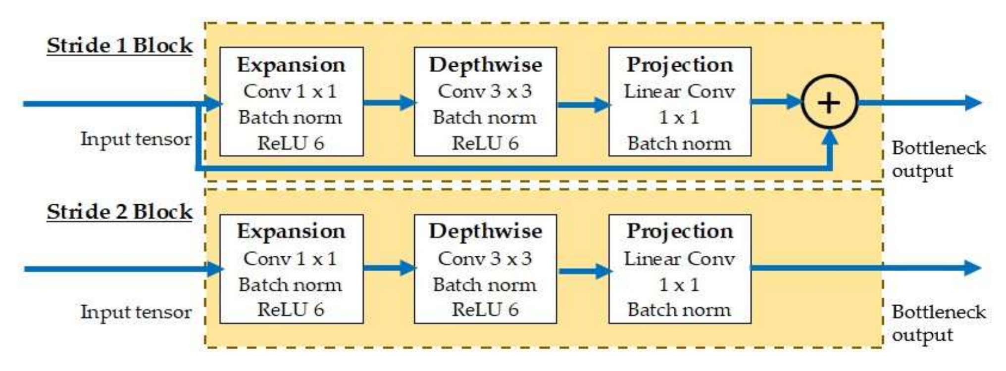
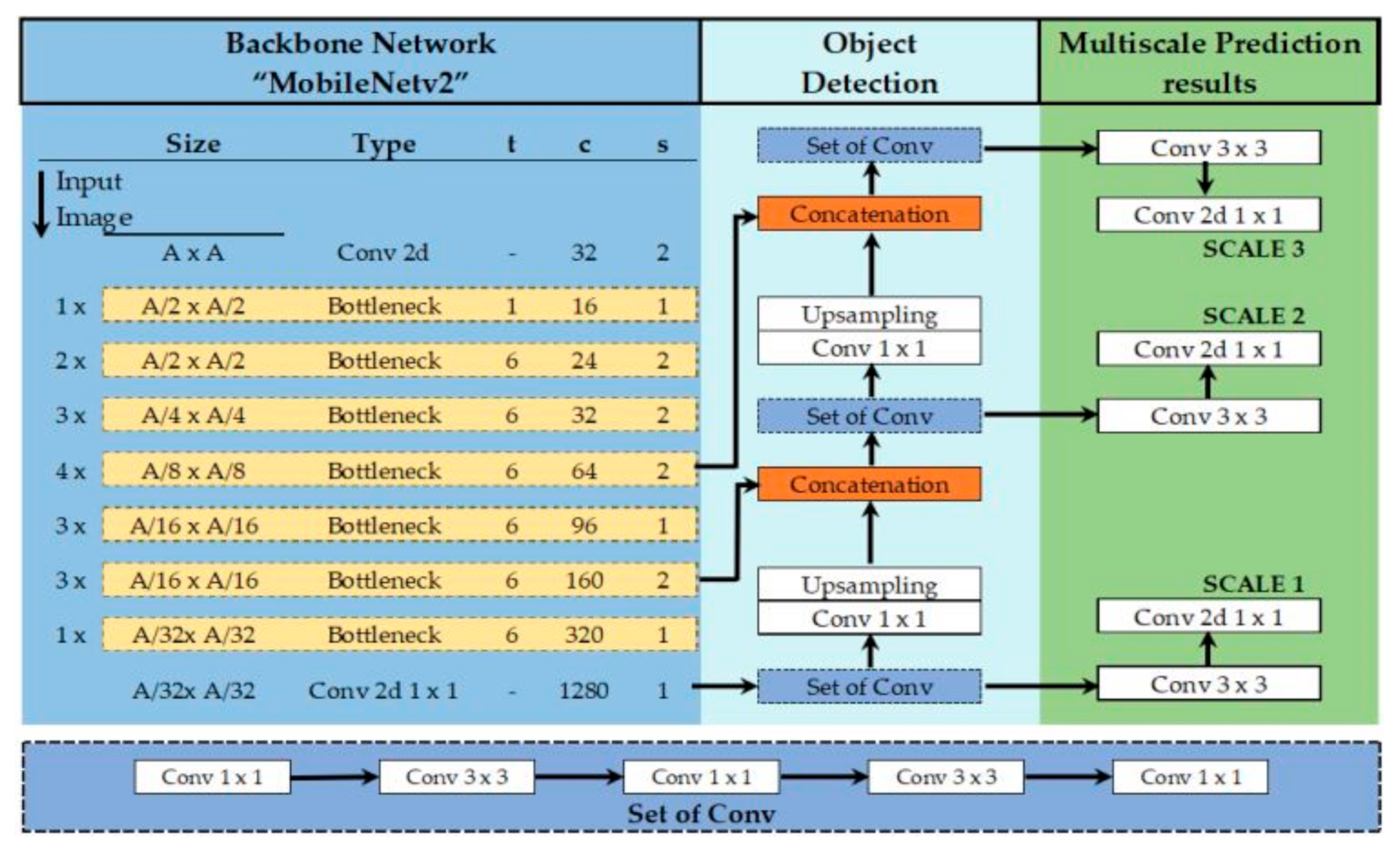
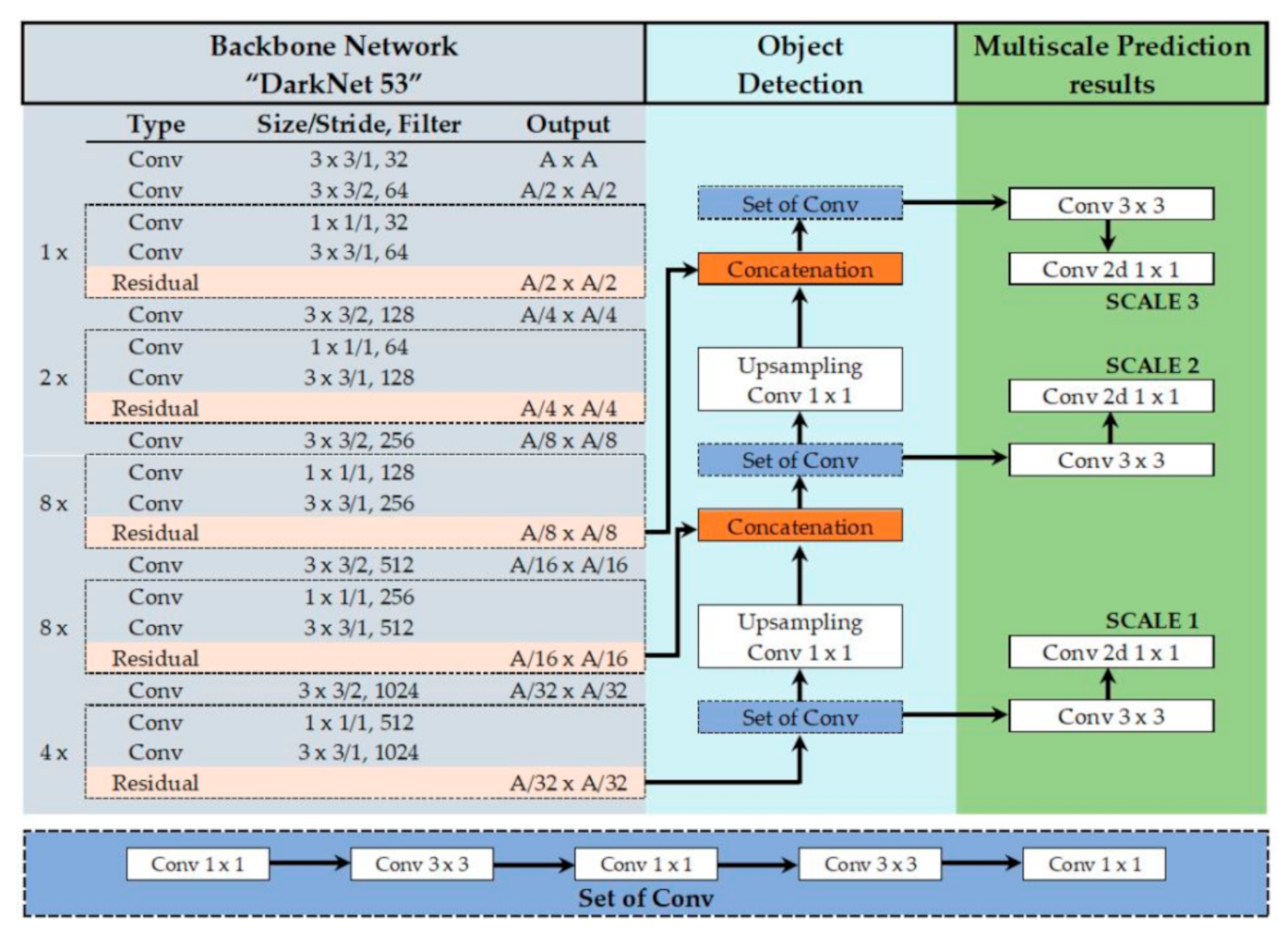
In this study, the YOLOv3 [25], as described thoroughly in Appendix A, is modified to develop a lightweight detection model. Following the physicochemical behavior of sample HNSs chemicals, a faster detection model was adopted by replacing DarkNet53 in the YOLOv3 framework with a lightweight MobileNetv2 [26] as a backbone architecture for feature extraction. With depthwise separable convolutions and inverted residual modules in the network, the MobileNetv2 architecture has fewer parameters, resulting in faster processing speed and requiring low computational power systems. MobileNetv2 utilizes the idea of linear bottleneck residual block to condense the data flowing through the network, which maintains the representation capability of the model. It has two types of residual blocks: Stride 1 consisting of a residual connection and stride 2 for downsizing, as shown in Figure 2. Each block holds three convolutional layers, an expansion layer with 1 × 1 convolution for uncompressing the input tensor size, followed by 3 × 3 depthwise convolution for data filtering, and finally projection layer with 1 × 1 pointwise convolution for compressing the data to bottleneck output. Each layer has ReLU 6 activation function, except for the projection layer to avoid adding non-linearity. Figure 3 represents the object detection algorithm by YOLOv3 with MobileNetv2 backbone architecture.
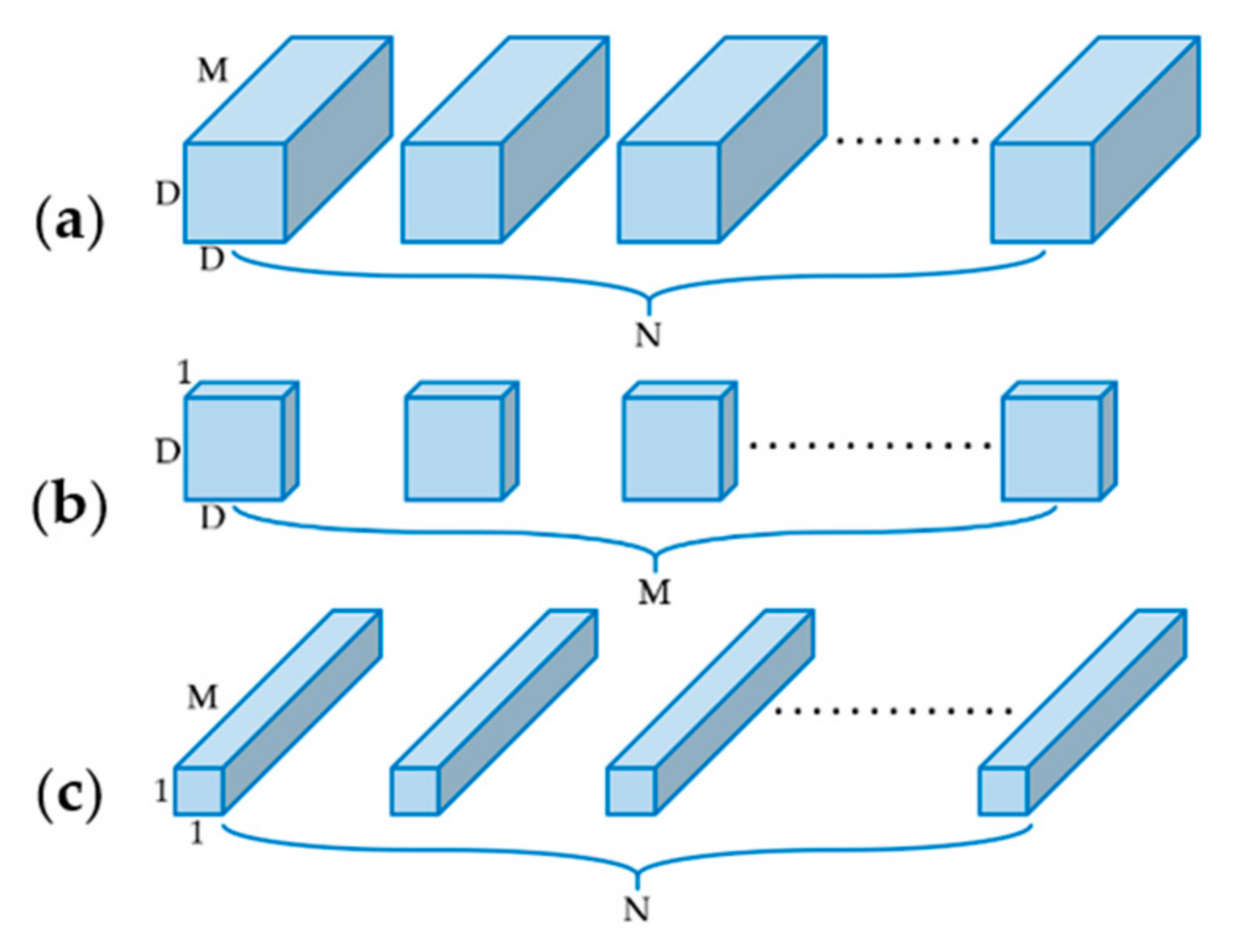
Based on regression, the lightweight YOLOv3 is a fully convolutional network that is constructed using depthwise separable convolution. After each convolutional layer, a batch normalization layer is added to improve model convergence speed and solve gradient explosion during backpropagation. In the depthwise separable convolutional network, the standard convolution filter is replaced by the depthwise separable filter and pointwise convolution filter, as shown in Figure 4.
The number of parameters of standard convolution filter and depthwise separable convolution filter can be calculated as follows:
Parameters (standard conv) = D × D × N × M
Parameters (depthwise conv) = D × D × M + N × M
Equation (3) represents the compression ratio of standard convolution and depthwise separable convolution filter. N and M represent the output and input feature maps, respectively.
2.2.1. Improved Loss Function
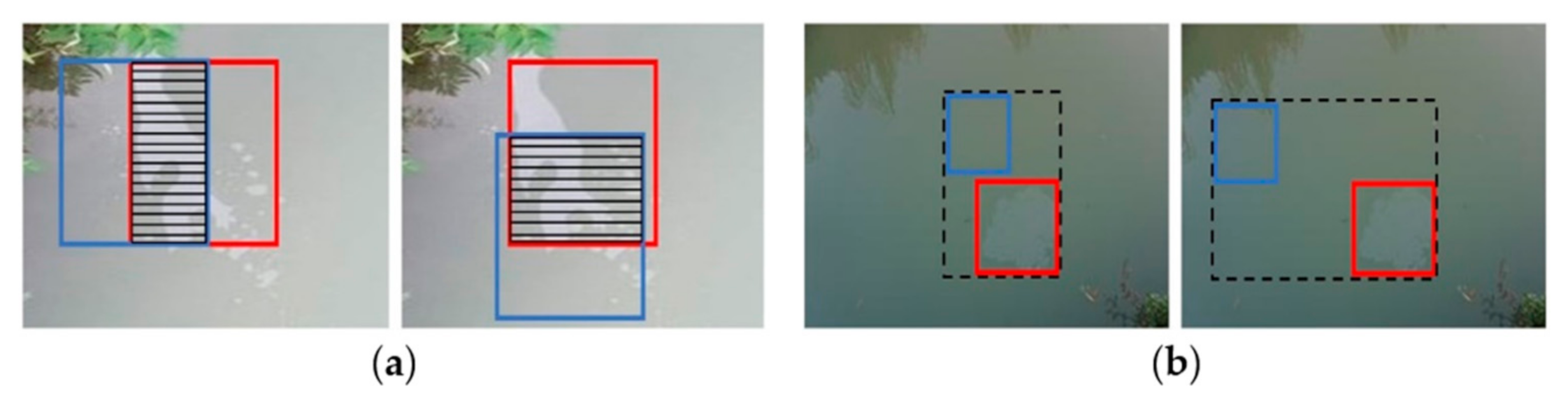
In YOLOv3, the evaluation index of object detection depends on IoU, which indicates the amount that the predicted bounding box overlaps with the ground truth bounding box. However, optimizing the loss function based on IoU calculations has significant complications. Suppose the bounding boxes overlap in differential geometry with the same intersection level. In this case, they will result in precisely the same IoU, but the bounding box regression is different, as shown in Figure 5a. In another case, if the predicted and ground truth bounding boxes do not intersect, then the resulting IoU value and gradient will be zero, which cannot optimize the loss function. IoU does not predict the loss due to the distance between predicted and ground truth bounding boxes. GIoU as a new bounding box regression loss function is adopted to address these shortcomings. The difference between IoU and GIoU is defined in Equations (4) and (5), as follows:
where A and B represent the bounding boxes, and C is the smallest circumscribed rectangle enclosing A and B. Depending on the distance between the bounding boxes, the value of IoU and GIoU ranges from [0, 1] to [−1, 1], respectively. In addition, the value of IoU and GIoU is near 1 when the predicted and ground truth bounding boxes overlap. If there is no overlap, the value of IoU is 0, and GIoU gradually approaches −1. Consequently, GIoU is a reasonable distance measurement index that focuses on non-overlapping areas. Figure 5b describes the GIoU variation of C with better and wrong predictions.
Total loss in the lightweight detection model can be calculated by substituting the bounding box regression loss based on GIoU in the YOLOv3 loss equation as in Appendix A.1, Equation (A2), as follows:
2.2.2. Anchor Box Generation
In YOLOv3, the evaluation index YOLOv3 utilizes the concept of anchor boxes while predicting the bounding box. These anchor boxes directly impact the speed and detection accuracy. There are nine anchor boxes in YOLOv3, which are (10, 13), (16, 30), (33, 23), (30, 61), (62, 45), (59, 119), (116, 90), (156, 198), and (373, 326) for the COCO dataset. In this work, nine anchor boxes produced by k-means clustering are (38, 23), (78, 52), (112, 84), (127, 117), (194, 98), (165, 139), (243, 155), (199, 205), and (297, 237).
3. Experimentation
3.1. Model Training
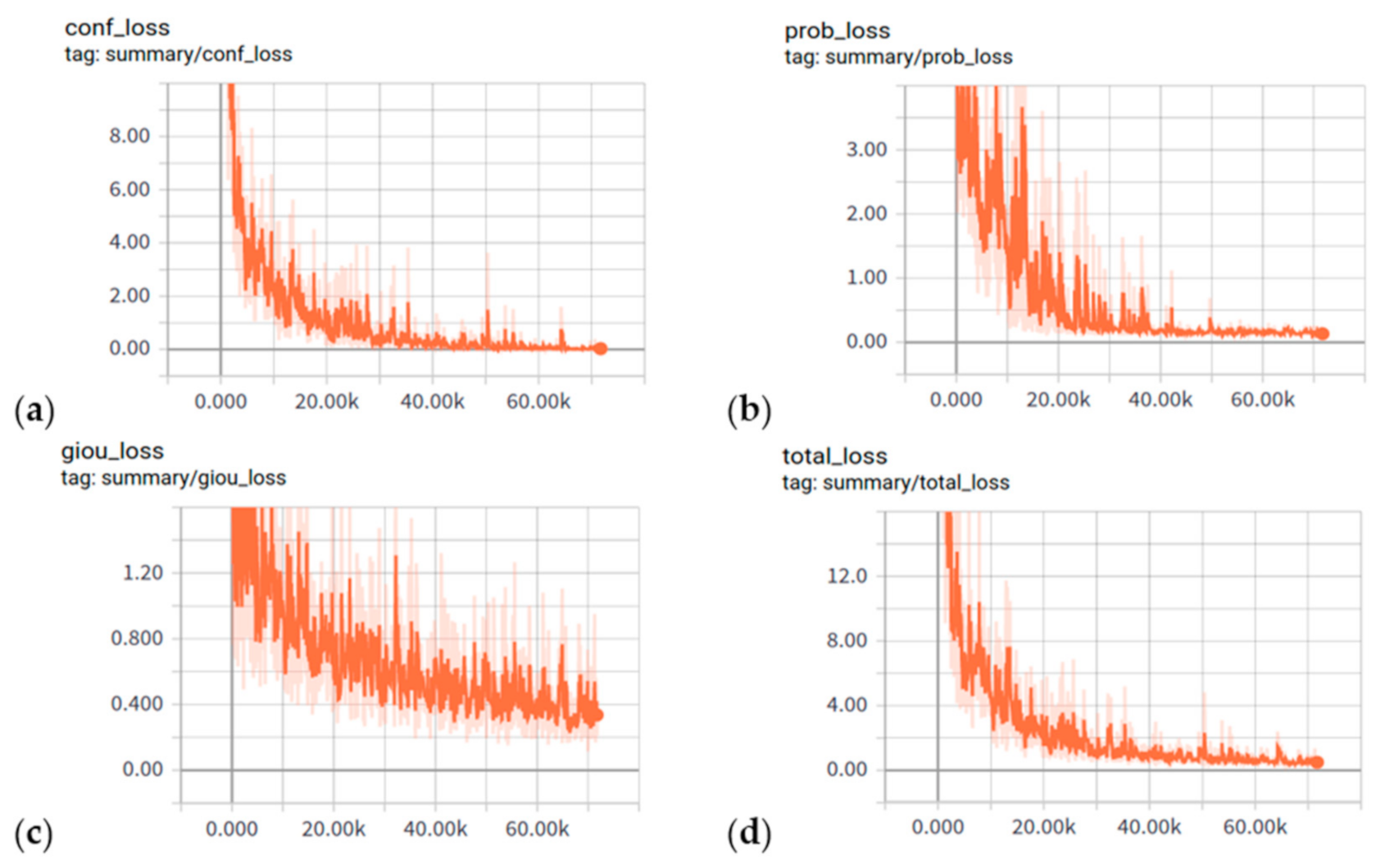
The experiments were performed by the DL open-source library TensorFlow 1.12, OpenCV 4.1.1, and coding was concluded with the high-level language python 3.5 on Ubuntu 18.04 operating system. The computational system included intel core i-7-7700, GPU GTX1080Ti with 12 GB of memory. Multiscale image resolution was performed during the training of the model, which changed the dataset resolution every 10 batches. The learning rate was set to change gradually during training to enhance the convergence of the model. The optimal values of hyperparameters as shown in Table 3 for training were selected through a grid search. Training loss curves of the models are presented in Figure 6.
3.2. Evaluation Protocols
To evaluate the proposed model for HNSs detection, a performance evaluation is conducted [38], and the following techniques were used to assess the model accuracy, which include IoU, precision (P), recall (R), average precision (AP), and mean average precision (mAP). In addition, to measure the efficiency and speed of the network, the detection time and the frame per second (FPS) were also evaluated.
The prime purpose is to calculate the IoU between the predicted bounding boxes and the ground truth. The test result will be true positive (TP) if IoU is higher than the 50% threshold, and false positive (FP) if the IoU value is less than the threshold. TP is the detection of an object correctly with a positive sample, and FP is the detection of an object negatively by accident of a positive sample. False negative (FN) shows that no targeted object in the image carries a positive sample. The precision (P) and recall (R) are calculated as follows:
The mAP is an extension of average precision (AP), where the average precision of every class is calculated.
4. Detection Results of the Proposed Model
Multiple distinct experiments were conducted on RGB and UV images for test detection of HNSs to better understand the behavior and evaluate the performance of the YOLOv3 lightweight model.
4.1. Spill Location Detection
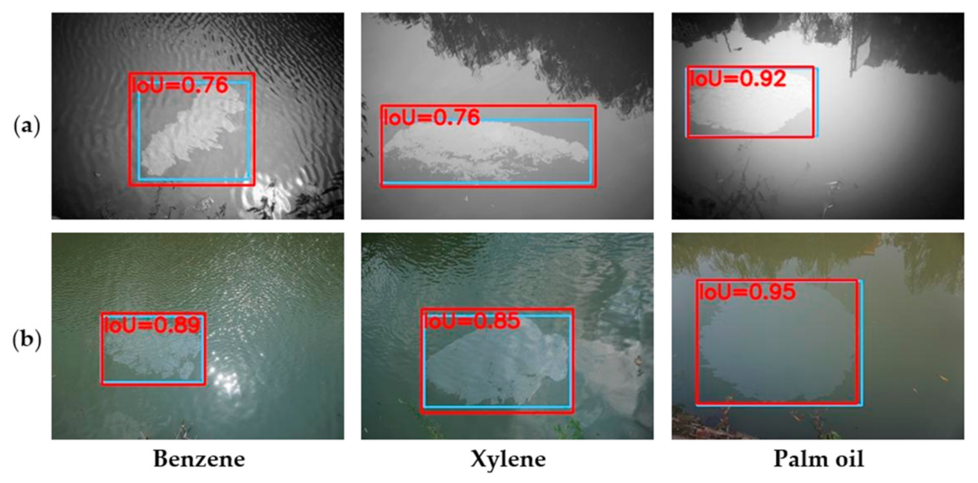
The test images were detected, and the IoU values were evaluated for UV and RGB images. The bounding box produced by the YOLOv3 lightweight model is shown in Figure 7. The aqua color is the ground truth of an object, and the red color is the predicted bounding box. The predicted boxes for three samples can be considered correct, as the average IoU values of all the samples is more than 50%. The model showed average IoU values of 86.57% and 80.43% for UV and RGB images. The average IoU values of detection explain that the bounding box regression loss function based on GIoU better fits the proposed YOLOv3 lightweight model. Moreover, the results conclude that the detection rate of palm oil has significantly better IoU values in both UV and RGB images.
4.2. Evaluation Based on Precision and Recall
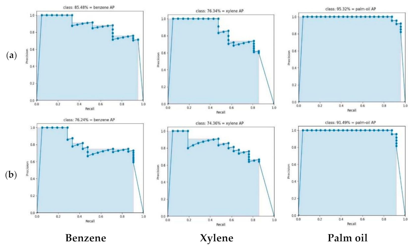
The precision–recall curve (PRC) is also one of the fundamental indexes to measure the effectiveness and accuracy of the object detection model. The PRC of sample HNSs, including UV and RGB images with the resolution of 608 × 608, is shown in Figure 8. The curves represent linear and better convergence of the proposed model. Of note, PRCs generated by UV images are overall better than RGB images. In UV images, palm oil with the highest AP scores (95.32%) has a perfect classification effect, followed by benzene (85.48%) and xylene (76.34%).
Similarly, AP scores of palm oil, benzene, and xylene in RBG images are 91.49%, 76.24%, and 74.36%, respectively. The results provided evidence that the precision of the proposed model had a transparent edge at a similar recall rate. Moreover, it specifies that the GIoU loss function has enhanced its performance.
4.3. Evaluation Based on Multiscale Resolution
The multiscale resolution technique is used in the YOLOv3 lightweight model. Significant variation in per class AP, mAP, detection time (D-time), and FPS can be observed from lower resolution to higher resolution, as shown in Table 4. This study provides substantial evidence of the influence of resolution on the detection behavior of the model. Moreover, it can be observed that overall detection results are improved using UV imaging.
4.4. Sample HNSs Spill Classification
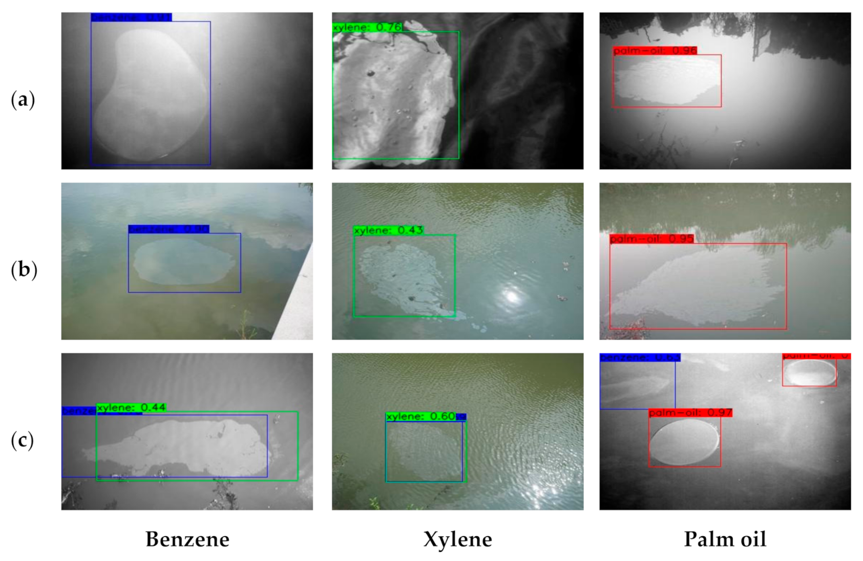
Figure 9 shows the classification results of three kinds of transparent HNSs spills in UV and RGB images by the YOLOv3 lightweight model. Sample spills in these images can be detected as undistinguishable targets via conventional procedures. The proposed model can classify the transparent spill with advanced imaging techniques and a robust feature extraction algorithm. Although the classification accuracy may differ a little in different circumstances, the sample images carry unalike ambient conditions containing similar objects, such as wave reflection and sun glitter, that are not detected as real targets.
In UV imaging, the transparent spill target has a more significant difference to the background that is ultimately helpful for the detection capabilities of the model. Moreover, the results proved that UV images attained more exceptional accuracy than the detection and classification of target spill in RGB images.
5. Discussion
To better evaluate the proposed YOLOv3 lightweight model, it is compared with the YOLOv3 baseline network trained from scratch with the HNSs dataset using the same training parameters as shown in Table 3. Unlike the YOLOv3 lightweight model, the baseline YOLOv3 network used the IoU regression loss function. A comparative analysis among the three models for HNSs detection is presented in Table 5. The results show that the proposed YOLOv3 lightweight model is computationally cost-effective, consuming about 9 times smaller data than the YOLOv3 baseline model. Further investigations revealed that the improved lightweight model resulted in comparable detection accuracy with faster image processing speed and around 3 times lower detection time than the YOLOv3 baseline model. Moreover, the proposed model surpassed the previous study by the authors of [24] in detection accuracy, FPS, and average detection time.
Although the proposed study has made progress in detecting transparent HNSs spills, it also resulted in false prediction as shown in Figure 9c. The encountered problems in the models’ results can be due to the following reasons:
- Overfitting problem caused by the small size of the dataset resulting in the detection model may not generalize well to unseen features in test images.
- Influence of ambient conditions, which may cause errors in detection. This problem can be solved by enhancing the generalization capability of the detection model by adding more training images.
6. Conclusions
The study proposed an improved and lightweight DCNN model to rapidly detect and classify HNSs spills. Due to the unavailability of publicly accessible data, a distinct and generic HNSs spill dataset is constructed, including UV (at 365 nm) and RGB images of benzene, xylene, and palm oil in different aquatic environments. The collected dataset is further augmented to meet the data volume requirement of the DCNN.
A DCNN named the YOLOv3 lightweight model is suggested, which is a modified version of YOLOv3. DarkNet53 backbone architecture is replaced by lightweight MobileNetv2, and bounding box regression loss based on GIoU is introduced in the network. The experiments show that the model is suitable for HNSs spill detection, which resulted in overall IoU of 82.57% and 68.43%, and mAP of 85.89% and 70.40% for UV and RGB images, respectively. The results also revealed that UV imaging is more apposite for the detection purpose of HNSs spills.
Following the physicochemical behavior of HNSs, which are transparent and highly volatile, the proposed model outperformed benchmark DCNN models in accuracy and detection speed. In addition, the model has 31 million parameters that are half of standard YOLOv3 and occupies 107.6 MB on disk, 9 times less than the YOLOv3 baseline model. The processing rate is 57 FPS, which is more than double of YOLOv3. Moreover, the proposed model is 3 times faster in detection, which rapidly detects spills in 11.9 ms on average.
Furthermore, to the best of our knowledge, the suggested model is one of the few reported studies using DCNN for HNSs spill detection. The model accurately and efficiently detects and classifies transparent HNSs spills in coarse conditions, such as wave reflections, water surface illumination, etc. Ultimately, the model can be utilized for swift detection, not only limited to HNSs spill detection on a large-scale, but also any other phenomenon requiring rapid and efficient detection using the lowest possible computational resources. Future studies will include the extension of the HNSs spill dataset by adding a variety of samples collected through monitoring the marine environment, which will enhance the detection efficiency of the model. Moreover, the proposed model will be implemented and tested on large-scale monitoring and mitigation of marine HNSs pollution.
Author Contributions
Conceptualization, methodology, and designing, S.R.M., K.R. and H.H.; software, validation, experimental analysis, and investigation, S.R.M., K.R., H.H. and R.A.N.; data curation, S.R.M., K.R., H.H. and A.A.; writing—original draft preparation, S.R.M., K.R. and H.H.; writing—review and editing, S.R.M., K.R., H.H., A.A. and H.S.; visualization, S.R.M., H.H. and H.S.; supervision and funding acquisition, H.H. and H.S. All authors have read and agreed to the published version of the manuscript.
Funding
This study was financially supported by the Key Research and Development Plan of Zhejiang Province, China (grant numbers 2021C03181, 2020C03012, 2019C02050), Major Science and Technology Project of Sanya (grant number SKJC–KJ–2019KY03), and the National Science Foundation of China (grant number 31801619).
Institutional Review Board Statement
Not applicable.
Informed Consent Statement
Not applicable.
Data Availability Statement
Data underlying the results presented in this paper are not publicly available since they are part of the ongoing work, but may be obtained from the authors later upon reasonable request.
Acknowledgments
The authors would like to express their gratitude to Hui Huang’s team for their contribution during HNSs image dataset development.
Conflicts of Interest
The authors declare no conflict of interest.
Appendix A
Appendix A.1. YOLOv3
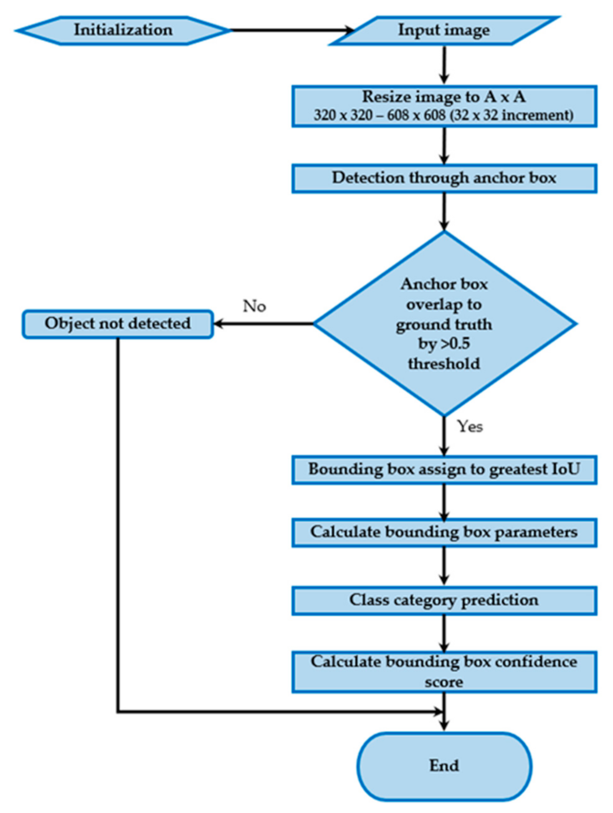
YOLOv3 is an end-to-end single-stage object detection (including target localization and classification) algorithm that encapsulates all of the steps in a single network. It considers object detection a regression problem by eliminating region proposal generation and feature resampling. Benefiting from single feed-forward CNN, YOLOv3 is significantly faster than other algorithms with comparable performance, taking the whole image to predict bounding box offsets to locate objects in the image and probabilities of object categories. The object detection workflow is shown in Figure A1.
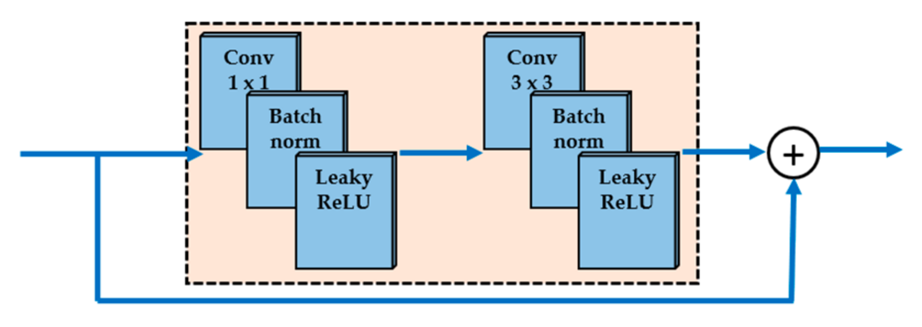
YOLOv3 is a deeper network based on backbone architecture, DarkNet53, with 53 convolution layers, including upsampling, route, detection, and residual units. There are five residual units in YOLOv3 that perform feature extraction, each using successive 1 × 1 and 3 × 3 convolution layers with skip connections. The skip connections are used to feed the output of the earlier layers to later layers by skipping some layers in between. Usually, this is done due to features extracted at earlier layers that are required later during the upsampling layer. Each convolution layer is followed by batch normalization and leaky ReLU layers for better convergence of feature maps and leaky ReLU layers. Gradient fading can be reduced to a minimum by introducing residual units in the network. The residual unit is shown in Figure A2.
YOLOv3 splits the input image into small S × S grids to perform object detection. The representative grid is responsible for detecting the object, if the center of an object falls in the grid field. These grids also locate the bounding boxes and later calculate the objectness score corresponding to these bounding boxes. The objectness score represents the probability that the object is located in the bounding box by calculating the IoU of the ground truth box and the predicted bounding box.
Briefly, the YOLOv3 model takes an input image first and resizes it to 320 × 320, which is randomly increased by 32 × 32 after certain successive epochs until a maximum resolution of 608 × 608 is achieved. After multiple layers of convolution, the image is downsampled 5 times. YOLOv3 makes detection predictions of targets in the last three downsampled layers. Unlike prior models, YOLOv3 detects an object at three scales by downsampling the feature maps to different levels. The feature map is downsampled by 8× at scale 3, 16× at scale 2, and 32× at scale 1 to detect small, medium, and big targets. Small feature maps providing deep semantic, and large feature maps providing more fine-grained information are resized, resulting in same size feature maps at different scales. The feature maps are fused together to detect targets. Finally, YOLOv3 uses multiscale features to detect and classify small objects and an independent logistic classifier rather than a softmax layer with improved mean average precision (mAP). The YOLOv3 network architecture is shown in Figure A3.
The loss function of YOLOv3 can be calculated as follows:
In the above equations, i represents the grid, j represents the bounding box predicted by the grid, is responsible for the existence of target object in grid i by the bounding box, s2 denotes the grid space where bounding boxes are present, x and y denote the actual and predicted coordinates of the bounding box, w and h represent the actual and predicted width and height of the bounding box, obj and noobj indicate the presence and absence of an object, represent the class of actual and predicted objects, indicate the actual and predicted probability scores, respectively. In the equations, the penalty coefficients and are also included to optimize the detection model’s bounding box regression loss and confidence loss. For the stability and enhanced convergence of the model, is usually taken as 5 to increase the weight of the bounding box localization and is taken as 0.5 to decrease the confidence loss by 50%, since the boxes do not contain any object.
Figure A1.
YOLOv3 object detection flow diagram.

Figure A2.
Residual unit of DarkNet53 consisting of convolutional, batch normalization, leaky ReLU layers, and a skip connection.
Figure A2.
Residual unit of DarkNet53 consisting of convolutional, batch normalization, leaky ReLU layers, and a skip connection.

Figure A3.
Illustration of YOLOv3 detection network architecture [39].
Figure A3.
Illustration of YOLOv3 detection network architecture [39].

References
- Harold, P.D.; De Souza, A.S.; Louchart, P.; Russell, D.; Brunt, H. Development of a risk-based prioritization methodology to inform public health emergency planning and preparedness in case of accidental spill at sea of hazardous and noxious substances (HNS). Environ. Int. 2014, 72, 157–163. [Google Scholar] [CrossRef] [PubMed]
- Michel, G.; Siemiatycki, J.; Désy, M.; Krewski, D. Associations between several sites of cancer and occupational exposure to benzene, toluene, xylene, and styrene: Results of a case-control study in Montreal. Am. J. Ind. Med. 1998, 34, 144–156. [Google Scholar] [CrossRef]
- Häkkinen, J.M.; Posti, A.I. Review of maritime accidents involving chemicals–special focus on the Baltic Sea. TransNav Int. J. Mar. Navig. Saf. Sea Transp. 2014, 8, 295–305. [Google Scholar] [CrossRef] [Green Version]
- Cunha, I.; Oliveira, H.; Neuparth, T.; Torres, T.; Santos, M.M. Fate, behaviour and weathering of priority HNS in the marine environment: An online tool. Mar. Pollut. Bull. 2016, 111, 330–338. [Google Scholar] [CrossRef] [PubMed]
- Cunha, I.; Moreira, S.; Santos, M.M. Review on hazardous and noxious substances (HNS) involved in marine spill incidents—An online database. J. Hazard. Mater. 2015, 285, 509–516. [Google Scholar] [CrossRef] [PubMed]
- Kim, Y.-R.; Lee, M.; Jung, J.-Y.; Kim, T.-W.; Kim, D. Initial environmental risk assessment of hazardous and noxious substances (HNS) spill accidents to mitigate its damages. Mar. Pollut. Bull. 2019, 139, 205–213. [Google Scholar] [CrossRef]
- Kirby, M.F.; Law, R.J. Accidental spills at sea–risk, impact, mitigation and the need for coordinated post-incident monitoring. Mar. Pollut. Bull. 2010, 60, 797–803. [Google Scholar] [CrossRef]
- Neuparth, T.; Moreira, S.; Santos, M.M.; Reis-Henriques, M.A. Review of oil and HNS accidental spills in Europe: Identifying major environmental monitoring gaps and drawing priorities. Mar. Pollut. Bull. 2012, 64, 1085–1095. [Google Scholar] [CrossRef]
- Yim, U.H.; Kim, M.; Ha, S.Y.; Kim, S.; Shim, W.J. Oil spill environmental forensics: The Hebei Spirit oil spill case. Environ. Sci. Technol. 2012, 46, 6431–6437. [Google Scholar] [CrossRef]
- Koeber, R.; Bayona, J.M.; Niessner, R. Determination of benzo [a] pyrene diones in air particulate matter with liquid chromatography mass spectrometry. Environ. Sci. Technol. 1999, 33, 1552–1558. [Google Scholar] [CrossRef]
- Li, C.-W.; Benjamin, M.M.; Korshin, G.V. Use of UV spectroscopy to characterize the reaction between NOM and free chlorine. Environ. Sci. Technol. 2000, 34, 2570–2575. [Google Scholar] [CrossRef]
- Hilmi, A.; Luong, J.H.T. Micromachined electrophoresis chips with electrochemical detectors for analysis of explosive compounds in soil and groundwater. Environ. Sci. Technol. 2000, 34, 3046–3050. [Google Scholar] [CrossRef]
- Alpers, W.; Holt, B.; Zeng, K. Oil spill detection by imaging radars: Challenges and pitfalls. Remote Sens. Environ. 2017, 201, 133–147. [Google Scholar] [CrossRef]
- Zhao, J.; Temimi, M.; Ghedira, H.; Hu, C. Exploring the potential of optical remote sensing for oil spill detection in shallow coastal waters-a case study in the Arabian Gulf. Opt. Express 2014, 22, 13755–13772. [Google Scholar] [CrossRef] [PubMed]
- Taravat, A.; Frate, F.D. Development of band ratioing algorithms and neural networks to detection of oil spills using Landsat ETM+ data. EURASIP J. Adv. Signal Process. 2012, 1, 1–8. [Google Scholar] [CrossRef]
- Al-Ruzouq, R.; Gibril, M.B.A.; Shanableh, A.; Kais, A.; Hamed, O.; Al-Mansoori, S.; Khalil, M.A. Sensors, features, and machine learning for oil spill detection and monitoring: A review. Remote Sens. 2020, 12, 3338. [Google Scholar] [CrossRef]
- Park, J.-J.; Park, K.-A.; Foucher, P.-Y.; Deliot, P.; Floch, S.L.; Kim, T.-S.; Oh, S.; Lee, M. Hazardous Noxious Substance Detection Based on Ground Experiment and Hyperspectral Remote Sensing. Remote Sens. 2021, 13, 318. [Google Scholar] [CrossRef]
- Huang, H.; Liu, S.; Wang, C.; Xia, K.; Zhang, D.; Wang, H.; Zhan, S.; Huang, H.; He, S.; Liu, C.; et al. On-site visualized classification of transparent hazards and noxious substances on a water surface by multispectral techniques. Appl. Opt. 2019, 58, 4458–4466. [Google Scholar] [CrossRef]
- Zhan, S.; Wang, C.; Liu, S.; Xia, K.; Huang, H.; Li, X.; Liu, C.; Xu, R. Floating xylene spill segmentation from ultraviolet images via target enhancement. Remote Sens. 2019, 11, 1142. [Google Scholar] [CrossRef] [Green Version]
- Han, Y.; Hong, B.-W. Deep learning based on Fourier convolutional neural network incorporating random kernels. Electronics 2021, 10, 2004. [Google Scholar] [CrossRef]
- Choi, J.; Kim, Y. Time-aware learning framework for over-the-top consumer classification based on machine- and deep-learning capabilities. Appl. Sci. 2020, 10, 8476. [Google Scholar] [CrossRef]
- Rew, J.; Park, S.; Cho, Y.; Jung, S.; Hwang, E. Animal movement prediction based on predictive recurrent neural network. Sensors 2019, 19, 4411. [Google Scholar] [CrossRef] [Green Version]
- Song, H.; Mehdi, S.R.; Zhang, Y.; Shentu, Y.; Wan, Q.; Wang, W.; Raza, K.; Huang, H. Development of coral investigation system based on semantic segmentation of single-channel images. Sensors 2021, 21, 1848. [Google Scholar] [CrossRef] [PubMed]
- Huang, H.; Wang, C.; Liu, S.; Sun, Z.; Zhang, D.; Liu, C.; Jiang, Y.; Zhan, S.; Zhang, H.; Xu, R. Single spectral imagery and faster R-CNN to identify hazardous and noxious substances spills. Environ. Pollut. 2020, 258, 113688. [Google Scholar] [CrossRef] [PubMed]
- Redmon, J.; Farhadi, A. Yolov3: An incremental improvement. arXiv 2018, arXiv:1804.02767. [Google Scholar]
- Sandler, M.; Howard, A.; Zhu, M.; Zhmoginov, A.; Chen, L.C. Mobilenetv2: Inverted residuals and linear bottlenecks. In Proceedings of the IEEE conference on computer vision and pattern recognition, Salt Lake City, UT, USA, 18–22 June 2018. [Google Scholar]
- Guo, H.; Wu, D.; An, J. Discrimination of oil slicks and lookalikes in polarimetric SAR images using CNN. Sensors 2017, 17, 1837. [Google Scholar] [CrossRef] [PubMed] [Green Version]
- Nieto-Hidalgo, M.; Gallego, A.-J.; Gil, P.; Pertusa, A. Two-stage convolutional neural network for ship and spill detection using SLAR images. IEEE Trans. Geosci. Remote Sens. 2018, 56, 5217–5230. [Google Scholar] [CrossRef] [Green Version]
- Guo, H.; Wei, G.; An, J. Dark spot detection in SAR images of oil spill using Segnet. Appl. Sci. 2018, 8, 2670. [Google Scholar] [CrossRef] [Green Version]
- Liu, B.; Li, Y.; Li, G.; Liu, A. A spectral feature based convolutional neural network for classification of sea surface oil spill. ISPRS Int. J. Geo-Inf. 2019, 8, 160. [Google Scholar] [CrossRef] [Green Version]
- Krestenitis, M.; Orfanidis, G.; Ioannidis, K.; Avgerinakis, K.; Vrochidis, S.; Kompatsiaris, I. Oil spill identification from satellite images using deep neural networks. Remote Sens. 2019, 11, 1762. [Google Scholar] [CrossRef] [Green Version]
- Yang, J.-F.; Wan, J.-H.; Ma, Y.; Zhang, J.; Hu, Y.-B.; Jiang, Z.-C. Oil spill hyperspectral remote sensing detection based on DCNN with multiscale features. J. Coast. Res. 2019, 90, 332–339. [Google Scholar] [CrossRef]
- Zeng, K.; Wang, Y. A deep convolutional neural network for oil spill detection from spaceborne SAR images. Remote Sens. 2020, 12, 1015. [Google Scholar] [CrossRef] [Green Version]
- Song, D.; Zhen, Z.; Wang, B.; Li, X.; Gao, L.; Wang, N.; Xie, T.; Zhang, T. A novel marine oil spillage identification scheme based on convolution neural network feature extraction from fully polarimetric SAR imagery. IEEE Access 2020, 8, 59801–59820. [Google Scholar] [CrossRef]
- Chen, Y.; Li, Y.; Wang, J. An end-to-end oil-spill monitoring method for multisensory satellite images based on deep 386 semantic segmentation. Sensors 2020, 20, 725. [Google Scholar] [CrossRef] [Green Version]
- Yekeen, S.T.; Balogun, A.-L.; Yusof, K.B.W. A novel deep learning instance segmentation model for automated marine oil spill detection. ISPRS J. Photogramm. Remote Sens. 2020, 167, 190–200. [Google Scholar] [CrossRef]
- Tzutalin. LabelImg. Git code (2015). Available online: https://github.com/tzutalin/labelImg (accessed on 19 January 2022).
- Rew, J.; Cho, Y.; Moon, J.; Hwang, E. Habitat Suitability Estimation Using a Two-Stage Ensemble Approach. Remote Sens. 2020, 12, 1475. [Google Scholar] [CrossRef]
- Zhao, H.; Zhou, Y.; Zhang, L.; Peng, Y.; Hu, X.; Peng, H.; Cai, X. Mixed YOLOv3-LITE: A lightweight real-time object detection method. Sensors 2020, 20, 1861. [Google Scholar] [CrossRef] [PubMed] [Green Version]
Figure 1.
Examples of sample spill images of three classes from the HNSs dataset collected at different locations under varying ambient conditions: (a) Single spectrum UV images of sample spills; (b) RGB images of sample spills.
Figure 1.
Examples of sample spill images of three classes from the HNSs dataset collected at different locations under varying ambient conditions: (a) Single spectrum UV images of sample spills; (b) RGB images of sample spills.

Figure 2.
Illustration of inverted bottleneck residual convolutional block of MobileNetv2.

Figure 3.
Definition of lightweight YOLOv3 detection model explaining the detection algorithm with MobileNetv2 backbone architecture (t, c, and s represent the expansion factor, number of output channels, and stride, respectively).
Figure 3.
Definition of lightweight YOLOv3 detection model explaining the detection algorithm with MobileNetv2 backbone architecture (t, c, and s represent the expansion factor, number of output channels, and stride, respectively).

Figure 4.
The architecture of depthwise separable convolutional network: (a) Standard convolution filter; (b) depthwise separable convolution filter; (c) pointwise convolution filter.
Figure 4.
The architecture of depthwise separable convolutional network: (a) Standard convolution filter; (b) depthwise separable convolution filter; (c) pointwise convolution filter.

Figure 5.
Description of overlapping and non-overlapping predicted and ground truth bounding boxes: (a) Bounding boxes overlapping with better (left) and wrong (right) regression; (b) the variation in C (large rectangle) with better (left) and wrong (right) predictions.
Figure 5.
Description of overlapping and non-overlapping predicted and ground truth bounding boxes: (a) Bounding boxes overlapping with better (left) and wrong (right) regression; (b) the variation in C (large rectangle) with better (left) and wrong (right) predictions.

Figure 6.
YOLOv3 lightweight model training loss curves: (a) Confidence loss; (b) probability loss; (c) GIoU loss; (d) total loss.
Figure 6.
YOLOv3 lightweight model training loss curves: (a) Confidence loss; (b) probability loss; (c) GIoU loss; (d) total loss.

Figure 7.
Examples of resulting IoU and bounding boxes generated by the YOLOv3 lightweight model: (a) Detection results based on UV images; (b) detection results based on RGB images.
Figure 7.
Examples of resulting IoU and bounding boxes generated by the YOLOv3 lightweight model: (a) Detection results based on UV images; (b) detection results based on RGB images.

Figure 8.
Precision and recall curves for three classes of sample spills detected by the YOLOv3 lightweight model: (a) PR curves based on UV images; (b) PR curves based on RGB images.
Figure 8.
Precision and recall curves for three classes of sample spills detected by the YOLOv3 lightweight model: (a) PR curves based on UV images; (b) PR curves based on RGB images.

Figure 9.
Classification of sample HNSs spills by the proposed model (blue, green, and red represent benzene, xylene, and palm oil, respectively): (a) Classification of spills in UV images; (b) classification of spills in RGB images; (c) example of false identification by model.
Figure 9.
Classification of sample HNSs spills by the proposed model (blue, green, and red represent benzene, xylene, and palm oil, respectively): (a) Classification of spills in UV images; (b) classification of spills in RGB images; (c) example of false identification by model.


Table 1.
Summary of reported studies using the applications of DCNN architectures for oil spill detection.
Table 1.
Summary of reported studies using the applications of DCNN architectures for oil spill detection.
| Year | Task | DCNN Architectures | Image Dataset | References |
|---|---|---|---|---|
| 2017 | Pixel-based spill classification | CNN with multiple convolutions and pooling layers | Radarsat-2 (SAR images) | [27] |
| 2018 | Object (spill) detection | 2-stage CNN | SAR images | [28] |
| Semantic segmentation | SegNet | Radarsat-2 (SAR images) | [29] | |
| 2019 | Pixel-based spill classification | 1-dimensional CNN | AVIRIS | [30] |
| Semantic segmentation | DeepLabv3 | Sentinel-1 (SAR images) | [31] | |
| Object (spill) detection | Multiscale features DCNN | Airborne hyperspectral images | [32] | |
| 2020 | Pixel-based spill classification | VGG-16 | ERS-1,2, COSMO SkyMed, ENVISAT (SAR images) | [33] |
| Pixel-based spill classification | CNN + SVM | Radarsat-2 (SAR images) | [34] | |
| Semantic segmentation | DeepLab + Fully connected conditional random field | QuickBird, Google Earth, and Worldview | [35] | |
| Instance segmentation | Mask R-CNN | Sentinel-1 (SAR images) | [36] |
Table 2.
Quantitative and exploratory data analysis of HNSs sample spills image dataset.
| Imaging Model | Spilled Chemical | Number of Images Captured at Different Locations | Total Training Images Augmentation (Yes/No) | Total Testing Images | |||
|---|---|---|---|---|---|---|---|
| Freshwater Lake | Canal | Artificial Pool | No | Yes | |||
| UV imaging | Benzene | 16 | 29 | 16 | 387 | 958 | 60 |
| Xylene | 11 | 28 | 31 | ||||
| Palm oil | 53 | 168 | 35 | ||||
| RGB imaging | Benzene | 09 | 37 | – | 468 | 1096 | 60 |
| Xylene | 14 | 40 | – | ||||
| Palm oil | 63 | 305 | – | ||||
Table 3.
Training parameters of HNSs spill detection model training.
| Model Training Parameters | Parameter Values |
|---|---|
| Learning rate | 1 × e−4 and 1 × e−6 |
| Total training epoch | 300 for the baseline model, 450 for lightweight YOLOv3 |
| Batch size | 4 and 6 |
| Image size | 320 × 320 to 608 × 608 |
| IoU threshold | 0.5 |
| Average decay | 0.995 |
| Gradient optimizer | Adam |
Table 4.
Analysis of proposed YOLOv3 lightweight model based on multiscale resolution.
| Image Size | Per Class AP (%) of UV Images | Per Class AP (%) of RGB Images | UV mAP | RGB mAP | Avg D-Time (ms) | FPS | ||||
|---|---|---|---|---|---|---|---|---|---|---|
| Benzene | Xylene | Palm Oil | Benzene | Xylene | Palm Oil | |||||
| 320 × 320 | 54.76 | 54.39 | 90.70 | 52.03 | 56.43 | 85.07 | 75.25 | 70.02 | 8.20 | 120 |
| 352 × 352 | 58.19 | 58.79 | 93.07 | 49.46 | 78.23 | 90.93 | 72.45 | 70.20 | 8.56 | 117 |
| 384 × 384 | 58.31 | 59.40 | 93.27 | 55.55 | 61.27 | 92.08 | 69.15 | 68.44 | 8.93 | 111 |
| 416 × 416 | 67.39 | 67.96 | 94.50 | 64.08 | 57.85 | 93.77 | 69.83 | 66.97 | 10.14 | 98 |
| 448 × 448 | 68.65 | 75.43 | 94.79 | 69.67 | 57.28 | 94.27 | 74.94 | 69.37 | 10.96 | 91 |
| 480 × 480 | 69.52 | 69.32 | 94.63 | 70.33 | 79.94 | 94.78 | 76.62 | 69.05 | 11.52 | 86 |
| 512 × 512 | 74.51 | 61.53 | 95.32 | 70.89 | 77.92 | 94.85 | 77.27 | 68.16 | 12.91 | 77 |
| 544 × 544 | 76.56 | 71.35 | 95.17 | 70.53 | 80.76 | 91.67 | 79.62 | 69.62 | 14.07 | 70 |
| 576 × 576 | 81.96 | 66.78 | 94.87 | 72.29 | 68.39 | 91.01 | 83.05 | 74.04 | 15.49 | 64 |
| 608 × 608 | 85.48 | 76.34 | 95.32 | 76.24 | 74.36 | 91.49 | 86.13 | 80.60 | 17.78 | 57 |
Table 5.
Comparison of proposed YOLOv3 lightweight model.
| Characteristic Parameters | Proposed Model | YOLOv3 Baseline | Faster RCNN by the Authors of [24] |
|---|---|---|---|
| mAP (UV) | 86.89% | 81.13% | 86.46% |
| mAP (RGB) | 72.40% | 66.94% | 66.73% |
| Parameters (million) | 31 | 61 | – |
| FPS | 57 | 23 | 5 |
| Average detection time (s) | 0.0119 | 0.0316 | 0.607 |
| Single Checkpoint size (Megabytes) | 107.6 | 985.1 | – |
Publisher’s Note: MDPI stays neutral with regard to jurisdictional claims in published maps and institutional affiliations. |
© 2022 by the authors. Licensee MDPI, Basel, Switzerland. This article is an open access article distributed under the terms and conditions of the Creative Commons Attribution (CC BY) license (https://creativecommons.org/licenses/by/4.0/).
Share and Cite
MDPI and ACS Style
Mehdi, S.R.; Raza, K.; Huang, H.; Naqvi, R.A.; Ali, A.; Song, H. Combining Deep Learning with Single-Spectrum UV Imaging for Rapid Detection of HNSs Spills. Remote Sens. 2022, 14, 576. https://doi.org/10.3390/rs14030576
AMA Style
Mehdi SR, Raza K, Huang H, Naqvi RA, Ali A, Song H. Combining Deep Learning with Single-Spectrum UV Imaging for Rapid Detection of HNSs Spills. Remote Sensing. 2022; 14(3):576. https://doi.org/10.3390/rs14030576
Chicago/Turabian StyleMehdi, Syed Raza, Kazim Raza, Hui Huang, Rizwan Ali Naqvi, Amjad Ali, and Hong Song. 2022. "Combining Deep Learning with Single-Spectrum UV Imaging for Rapid Detection of HNSs Spills" Remote Sensing 14, no. 3: 576. https://doi.org/10.3390/rs14030576
Note that from the first issue of 2016, this journal uses article numbers instead of page numbers. See further details here.