

The Atmospheric Correction of COCTS on the HY-1C and HY-1D Satellites
by
 , ,
, ,
Zhihua Mao
1,2,*,
Yiwei Zhang
1,
Bangyi Tao
1,
Jianyu Chen
1,2,
Zengzhou Hao
1,
Qiankun Zhu
1 and
Haiqing Huang
1 1
State Key Laboratory of Satellite Ocean Environment Dynamics, Second Institute of Oceanography, Department of Natural Resources, 36 Bochubeilu, Hangzhou 310012, China
2
School of Oceanography, Shanghai Jiao Tong University, 1954 Huashan Road, Shanghai 200240, China
*
Author to whom correspondence should be addressed.
Remote Sens. 2022, 14(24), 6372; https://doi.org/10.3390/rs14246372
Submission received: 25 July 2022
/
Revised: 13 December 2022
/
Accepted: 13 December 2022
/
Published: 16 December 2022
(This article belongs to the Special Issue Validation and Evaluation of Global Ocean Satellite Products)
Abstract
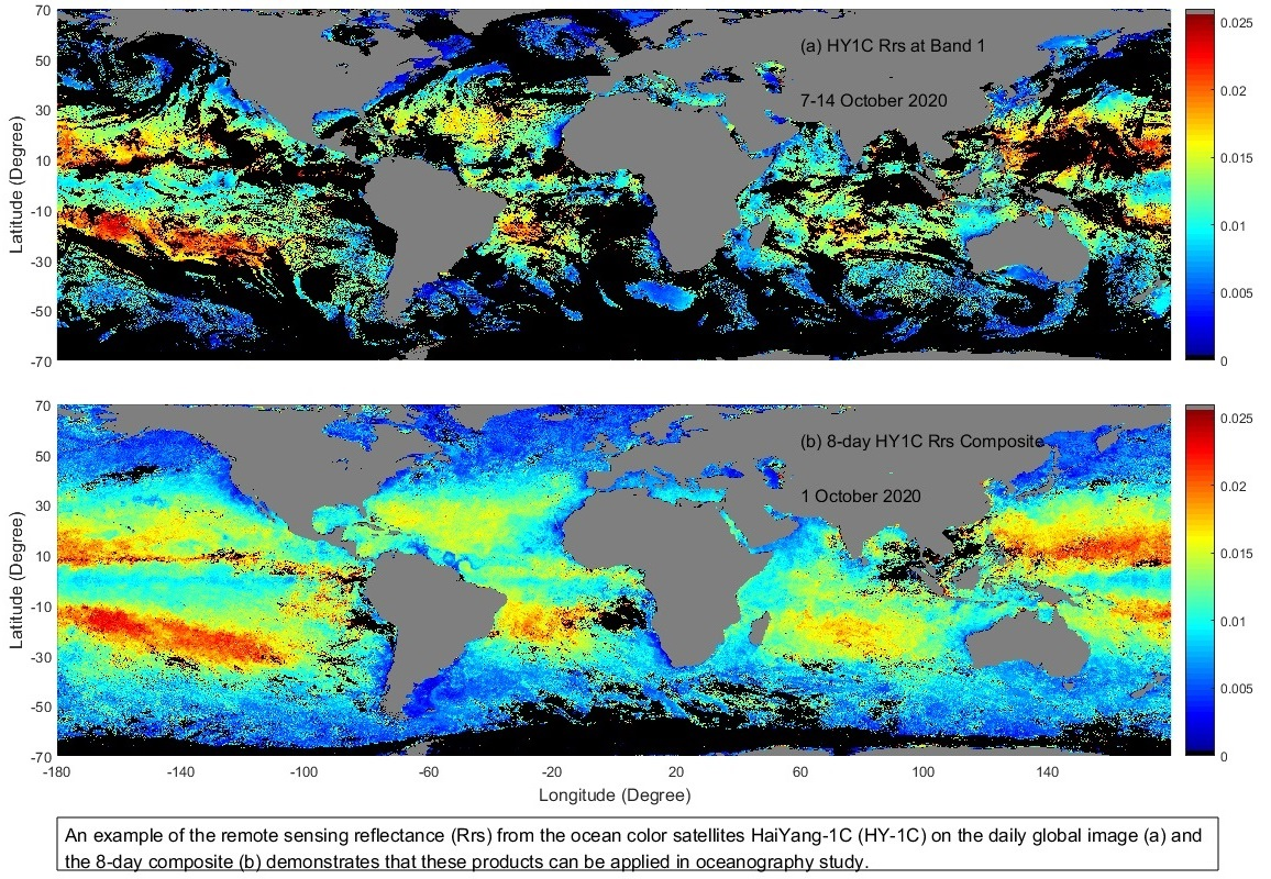
:The data quality of the remote sensing reflectance (Rrs) from the two ocean color satellites HaiYang-1C (HY-1C) and HaiYang-1D (HY-1D) and the consistency with other satellites are critical for the products. The Layer Removal Scheme for Atmospheric Correction (LRSAC) has been applied to process the data of the Chinese Ocean Color and Temperature Scanner (COCTS) on HY-1C/1D. The accuracy of the Rrs products was evaluated by the in situ dataset from the Marine Optical BuoY (MOBY) with a mean relative error (MRE) of −1.56% and a mean absolute relative error (MAE) of 17.31% for HY-1C. The MRE and MAE of HY-1D are 1.05% and 15.68%, respectively. The comparisons of the global daily Rrs imagery with the Moderate Resolution Imaging Spectroradiometer (MODIS) on Terra show an MRE of 10.94% and an MAE of 21.38%. The comparisons between HY-1D and Aqua exhibit similar results, with an MRE of 13.31% and an MAE of 21.46%. The percentages of valid pixels of the global daily images of HY-1C and HY-1D are 32.3% and 32.6%, much higher than that of Terra (11.9%) and Aqua (11.9%). The gaps in the 8-day composite images have been significantly reduced, with 83.9% of valid pixels for HY-1C and 85.4% for HY-1D, which are also much higher than that of Terra (52.9%) and Aqua (50.9%). The gaps due to the contamination of sun glint have been almost removed from the 3-day composite imagery, with valid pixels of 63.5% for HY-1C and 65.6% for HY-1D, which are higher than that of the 8-day imagery of Terra and Aqua. The patterns of HY-1C imagery exhibit a similarity with those of HY-1D, but they are different on a pixel scale, mainly due to the changes in the ocean dynamic features within 3 h. The evaluations of the COCTS indicate that the imagery of HY-1C/1D can be used as a kind of standard product.
Keywords:
atmospheric correction; ocean color remote sensing; evaluation; LRSAC; COCTS; HY-1C; HY-1D; MODIS; MOBY
1. Introduction
The Haiyang-1C (HY-1C) satellite, launched on 7 September 2018, is China’s third ocean color satellite and is the first operational one, as both HY-1A and HY-1B were the experimental satellites [1]. The HY-1D, with the same payloads as HY-1C, was launched on 11 June 2020 [2]. The HY-1C is the morning satellite and the HY-1D is the afternoon satellite equipped with the Chinese Ocean Color and Temperature Scanner (COCTS), Coastal Zone Imager (CZI), Ultraviolet Imager (UVI), Satellite Calibration Spectrum (SCS) and Automatic Identification System (AIS). The UVI, SCS and AIS are the new sensors comparing to HY-1A/1B. The specifications of COCTS and CZI have been improved compared to those on HY-1A/1B. The COCTS has eight visible channels for ocean color remote sensing and two infrared bands for the sea surface temperature [3,4]. The layer removal scheme for atmospheric correction (LRSAC) was used to process the COCTS data to obtain the spectral remote sensing reflectance (Rrs) products [5]. The performance of these products is critical to deriving the ocean biological and biogeochemical parameters because any results derived from Rrs are subject to significant uncertainty [6].
As residual errors in atmospheric correction (AC) can introduce large uncertainties in Rrs estimates, many previous works have been conducted to evaluate the performance of Rrs products from various AC algorithms of ocean color satellites [7,8,9]. Doxani et al. tested a wide range of AC algorithms and highlighted the strengths and limitations of each algorithm over different land cover types [7]. Wei et al. assessed the NIR-short-wave infrared (NIR-SWIR) approach among the four AC algorithms and produced the most robust Rrs estimates from Landsat 8 [8]. Ilori et al. evaluated the performances of four different AC algorithms to determine which method produces the most robust Rrs products in shallow coastal waters [9]. To improve the quality of Rrs products, many new AC approaches have been developed with the support of various characteristics of the satellite remote sensing data for different ocean regions [10,11,12,13,14,15,16,17].
The performance of the standard Rrs products from the operational AC algorithm for the Moderate Resolution Imaging Spectroradiometer (MODIS) has been well validated and proved to be consistently of high quality and stable long term [18,19,20,21]. Goyens et al. used four AC algorithms to compare the accuracy of MODIS products [18]. Carswell et al. evaluated the performance of MODIS-Aqua products from the three AC methods [19]. These products were used as benchmarks or references for the evaluation of Rrs produced by HY-1C/1D, especially the consistency evaluation of COCTS-retrieved products, which is critical for some long-term studies [22]. The consistency of ocean color products was evaluated between the Visible Infrared Imaging Radiometer Suite (VIIRS) on the Suomi National Polar-orbiting Partnership (SNPP) and the National Oceanic and Atmospheric Administration (NOAA)-20 [23]. In fact, this “satellite–satellite” comparison methodology was inspired by the cross-calibration technique for satellite sensors [24,25,26,27] and is used to evaluate the consistency of COCTS-retrieved products with those of MODIS.
The atmospheric correction plays a critical role in satellite remote sensing, and many algorithms have been developed. One great advance was the scheme partitioning the satellite-received signal into atmospheric and oceanic components [28]. However, it is not suitable that these components are linearly partitioned because they are actually coupled among them. A Layer Removal Scheme for Atmospheric Correction (LRSAC) model was developed to use some nonlinear equations to remove the effects of each layer from the satellite-received radiance using a step-by-step procedure [5]. The LRSAC model was used to process the COCTS data on HY-1C and HY-1D.
Although China launched the first ocean color satellite (HY-1A) twenty years ago, the available data of HY-1A and HY-1B were very limited. Now, all remote sensing data of HY-1C and HY-1D are available for free from the website, and other data from new powerful satellites will also be available soon due to the approval of the proposal for these new satellites. The performance of the satellite-retrieved products becomes critical for the time series studies with other satellites. The paper starts with descriptions of satellite data and the AC scheme for deriving Rrs productions of COCTS. Then, the in situ Rrs from the Marine Optical BuoY (MOBY) was used to evaluate the accuracy of products from HY-1C/1D. Next, the performance of the global daily and 8-day composite Rrs imagery of HY-1C was evaluated by Terra, and that of HY-1D was evaluated by Aqua. Finally, we discussed the effects of reducing the coverage of the sun glint contamination by the merged imagery of HY-1C/1D on the same day, the coverage of valid pixels in the 3-day composite imagery for the replacement of 8-day composite products, the spectral variations of Rrs at different bands and temporal changes within 3 h across the ocean dynamic features for the uncertainty in the evaluations of satellite-retrieved products.
2. Materials and Methods
2.1. Satellite Data and In Situ Data
The remote sensing data of COCTS on HY-1C/1D are available from the website (https://osdds.nsoas.org.cn/ (accessed on 30 December 2021)). Each file contains a record of about 5 min of satellite data. A total of 148,270 L1B files of HY-1C, with the period of 11 September 2018 to 31 May 2021, were downloaded. The downloaded HY-1D data include a total of 20,915 L1B files from 16 June 2020 to 31 October 2020. These files are processed to obtain the Rrs products using the LRSAC model [5].
The global satellite-retrieved Rrs imagery of MODIS on Terra and Aqua was downloaded from the NASA Ocean Color website (http://oceancolor.gsfc.nasa.gov (accessed on 20 January 2022)). This imagery is used to evaluate the performance, and Table 1 lists the comparison of some specifications between MODIS and COCTS. The atmospheric correction algorithm was proposed on the near-infrared (NIR) method [28], and two SWIR bands were used instead of NIR bands to compute the aerosol epsilon in turbid waters [29]. An iterative procedure is applied for the implementation of the method, and the iteration will not end until the relative difference of Rrs between the satellite-retrieved imagery and a bio-optical model is less than 2% at the red band [13]. As the wavelengths of MODIS are different from those of COCTS, the values of Rrs were adjusted by the wavelengths of the two sensors using the distance weight method:
where is the adjusted value of Rrs with the same wavelength of COCTS. and are the two Rrs values with the two nearest bands of MODIS, and their wavelengths are used to compute the term .
From Table 1, it can be seen that the central wavelength of eight COCTS visible bands is close to that of the ocean color bands of MODIS, but the bandwidth of each band is wider than that of MODIS, and the Signal-to-Noise Ratio (SNR) is lower than that of MODIS. These limitations of specifications may influence the data quality of COCTS and need to be improved for the new ocean color satellites. The spatial resolution of one COCTS pixel at nadir is about 1.1 by 1.1 km, which is similar to that of MODIS ocean color bands. The Swath of COCTS at the Equator is wider than 2900 km, which is much higher than that of MODIS (2330 km).
The MOBY is a radiometric observatory that served as the primary sea surface calibration site for many ocean color satellite missions, providing calibrated Rrs from the spectral upwelling radiance and downwelling irradiance at different depths [30]. The data were downloaded from the Moss Landing Marine Laboratories (MLML) MOBY data archive (https://www.mlml.calstate.edu/moby (accessed on 25 January 2022)). Actually, these in situ measurements of Rrs provide a nice dataset for evaluating the accuracy of the satellite-retrieved values of HY-1C/1D. The Rrs was obtained from the hyperspectral instruments, which can be accurately changed to the values on the wavelengths of COCTS using the spectral response functions of the sensor. Normally, the reflectance of MOBY was measured three times in one day at morning, noon and afternoon time, respectively. The morning time is around 10:30 a.m. local time, which is almost the same as the overpass time of HY-1C. The afternoon is around 1:30 p.m., which is almost the same as that of HY-1D. Therefore, it provides an ideal condition for the time window of the matchups. The reflectance measured at noon time was used when the above measurements were not available. The continuous daily measurements of MOBY also provide many matchups during a long time period. A total of 728 spectra were selected for HY-1C during the period from 10 September 2018 to 31 May 2021, and 57 spectra were used for HY-1D during the period from 16 June 2020 to 31 October 2021.
2.2. The Atmospheric Correction Scheme of COCTS on HY-1C/1D
Traditionally, the satellite signal is linearly partitioned into several components, but these components are coupled with each other. They are decoupled one-by-one using the nonlinear approach in the LRSAC model based on the five-layer structure according to the sunlight radiative transfer path in the Sun-Earth-satellite system [5]. The first step is to remove the atmospheric absorption of Layer 1 from the satellite :
where is the sensor spectral wavelength, is the Rrs at the top of Layer 2 and is the transmittance of total gaseous absorption, which includes ozone, oxygen, water vapor and carbon dioxide [31]. The reflectance at the top of Layer 3 ( ) is obtained by the removal of the Rayleigh scattering reflectance:
where , and are the Rrs, transmittance and the downward spherical albedo of the Rayleigh layer, respectively. These values are computed from the Rayleigh look-up-tables (LUTs) generated by the 6SV (Second Simulation of a Satellite Signal in the Solar Spectrum, a vector version 3.2) with ancillary wind speed data and air mass correction based on the ancillary surface pressure data [32,33]. Similarly, the surface reflectance is obtained from the removal of the aerosol scattering reflectance:
where , and are the Rrs, transmittance and the downward spherical albedo of the aerosol layer, respectively. These values are computed from the aerosol LUTs of multiple scattering using the 6SV code. The is obtained from the removal of the reflection of sun glint and whitecaps:
where and represent the Rrs of the surface glint in the specular direction and that contributed by whitecaps and foams on the surface [34]. These values are calculated using Fresnel theory and a statistical water surface model [35,36]. It should be noted that all of the above equations are dependent on pixel-by-pixel observing geometry (the solar zenith angle, sensor zenith angle and relative azimuth angle).
2.3. The Evaluation Method
The accuracy of Rrs may be estimated by two statistical indices: the systematic error represented by the mean relative error (MRE) and the random error defined by the mean absolute relative error (MAE), the root mean square (RMS) and the coefficient of determination (R2) [5]. As values of MRE and MAE are easily influenced by some pairs with large relative errors (RE), the median percent difference (MPD) and median absolute percent difference (MAD) are also used for the evaluation [19].
The matchup exercise should be carefully performed before the comparison of data from different sources. For the comparison of satellite Rrs products between COCTS and MODIS, the matchups are based on one pixel scale due to the similar spatial resolution of about 1 km. The overpass time of HY-1C is around 10:30 a.m. local time, which is close to that of Terra. The overpass time of HY-1D is around 1:30 p.m., which is close to that of Aqua. Therefore, the products of Terra are used to evaluate those of HY-1C, and those of Aqua are used for HY-1D. To make the matchup procedure easy, all data are projected into the daily global images with a spatial resolution of 4 by 4 km. The matchup approach was plain on the condition of both valid pixels of the two images on the same locations, which excluded the pixels flagged with land, clouds, stray light, sun glint and atmospheric correction failure. Other conditions such as the spatial window of several pixels and the filtering criteria of the coefficient of variation for homogeneity are not used in our evaluation.
The time window of COCTS and MOBY was set within 2 h for the matchups, ensuring that the measurements of MOBY at noon time can be used when the measurements at the morning or the afternoon were not available. All COCTS data were projected into the same region, with a spatial resolution of 1 by 1 km. The location at the MOBY site was the center of the region, and only the valid value of one pixel at the center was used for the matchups.
3. Results
3.1. Validation by MOBY Measurements
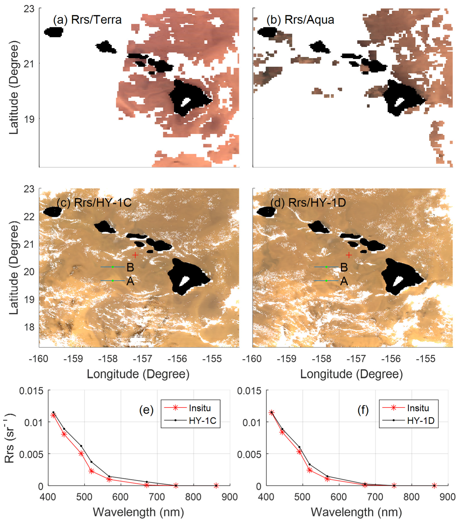
The L1B file of HY-1C on 6 October 2020 was selected and projected into the MOBY region with latitudes of 17–23 degrees and longitudes of −160 to −140 degrees, as shown in Figure 1c, which is a pseudo image of Bands 1–3. The MOBY site is marked as the red cross, and Figure 1e shows the comparison of Rrs at COCTS/HY-1C wavelengths between the MOBY-measured and satellite-retrieved images. The image in Figure 1c exhibits patterns of ocean dynamic features, with two blue lines to demonstrate the structures of spectra. The composite image of HY-1D is shown in Figure 1d, with the spectra comparison in Figure 1f. In comparison, the images from MODIS on Terra and Aqua on the same day are also shown in Figure 1a,b, respectively. The pixel scale of MODIS in Figure 1 is about 4 by 4 km, and that of COCTS is about 1 by 1 km.
The presence of clouds is the main factor producing invalid pixels of satellite images. The images in Figure 1 are relatively good, with a few coverages of clouds which are marked as white. The percentages of clouds in the two images are 17.8% for HY-1C and 20.2% for HY-1D. The distributions of clouds change from mornings to afternoons, and the merged image on the same day can significantly reduce the coverage of clouds (5.6%). The patterns of some ocean dynamic features can be identified from the image structures, and the distribution of the features in the HY-1C image exhibit similarity with those of HY-1D. It demonstrates that some ocean circulations can still be identified even with areas partly covered by clouds. Of course, the patterns of the merged image can reveal more details of the dynamic ocean features.
The comparison of the spectra shows that the satellite-retrieved reflectance is close to that of the in situ measurements. However, some values are still relatively large at some bands. In fact, the measurements of spectra from MOBY are relatively stable, but the differences at Band 4 reach higher than 10% between mornings and afternoons. The differences at Band 6 become much larger due to the small magnitudes of the Rrs at longer wavelengths in the open ocean. A small variation in the magnitude can easily lead to an RE value higher than 100%, which significantly affects the result of statistical computation.
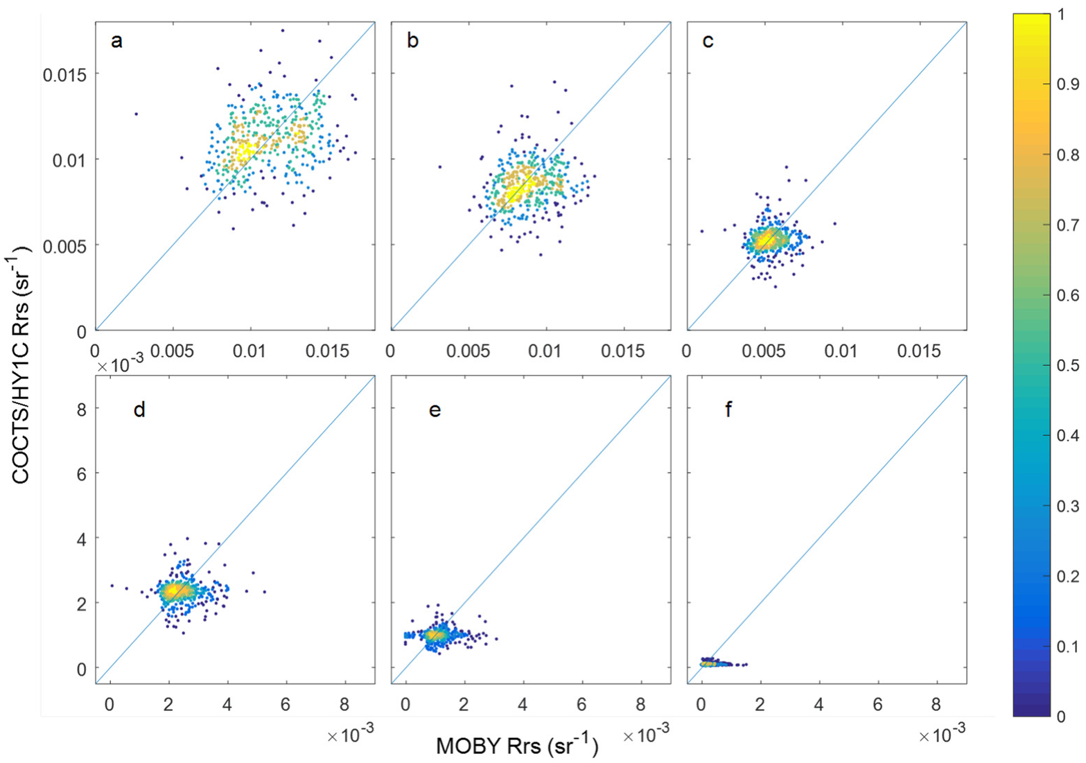
The matchups were established from the MOBY measurements at mornings and the valid pixels of the HY-1C at the MOBY site on the same day, obtaining a total of 469 pairs, as shown in Figure 2. All matchups at six bands were displayed to examine the robust performance of the satellite-retrieved products.
Figure 2 shows that most dots fall around the 1:1 line, indicating that the satellite-retrieved Rrs values agree reasonably with those from the MOBY measurements. Each subfigure exhibits a concentrated cluster of data pairs with the center located at the 1:1 lines, indicating that the systematic errors of satellite-retrieved Rrs at six bands are relatively small.
Due to the independent distributions of dots in Figure 2, it is reasonable to display all matchups to check the robust performance of the algorithm, but the statistical results may be influenced by some pairs with large RE values. The largest RE of one pair is higher than 1865%, and values of some pairs become invalid due to the zero of the in situ Rrs at Band 6. The value of MRE will increase by 3.84% when the pair with the largest RE takes part in computing; the statistics and the MRE value will increase to 39.7% if the number of matchups decreases to 47. It is obvious that the results of MRE deviating from the actual bias of the satellite-derived Rrs from some pairs with large RE values. To reflect the actual situation of the relative error, the pairs with RE values higher than 100% are taken as outliers and excluded from the statistical calculations in Table 2. For MPD and MAD, all matchups are included in the computation.
From Table 2, the mean values of the satellite-retrieved Rrs are close to those of the MOBY measurements at the six bands. The MRE values vary around 5%, with a mean of −1.56%, which are close to those of MPD, except for Band 6. The MAE values vary around 15%, with a mean of 17.31%, which are close to those of MAD, except for Band 6. The RMS value at Band 6 is small (3.93 × 10⁻⁵ sr−1), and the largest RMS is Band 1 (0.00227 sr−1), which is consistent with the mean values of reflectance. The percentages with an RE higher than 100% are 0.43%, 0.64%, 0.64%, 1.92%, 8.53% and 68.87% for Bands 1–6, respectively, indicating that the RE values of most pairs at Band 6 are higher than 100%. It causes the number of pairs significantly reduces from 455 at Band 1 to 99 at Band 6. This demonstrates that both MAD and MPD at Band 6 are much higher than MRE and MAE. As the magnitudes of Rrs at Band 6 are only about 1% of those at Band 1, the magnitudes at different bands are the important factors affecting the result of the relative errors.
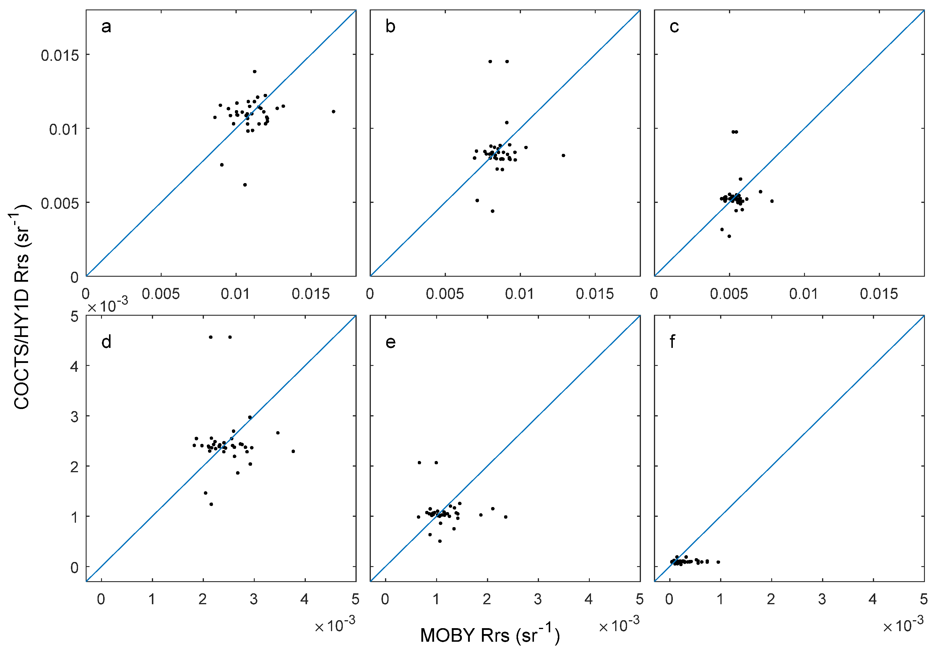
Similarly, the matchups were established from the MOBY measurements at around 13:30 and the valid pixel of the COCTS/HY-1D on the same day. A total of 38 pairs were obtained, and all pairs are shown in Figure 3.
Figure 3 shows that most matchups are distributed around the 1:1 line, indicating that the satellite-retrieved Rrs of COCTS/HY-1D agree well with those from the MOBY measurements. All matchups are used to compute the values of MPD and MAD, while the pairs with an RE higher than 100% are excluded from the computation of other statistical metrics in Table 3.
From Table 3, it can be seen that the mean values of HY-1D Rrs are close to those of MOBY at six bands. The MRE values vary from −0.25% at Band 5 to 12.61% at Band 6, with a mean of 1.05%. The MPD values are close to those of MRE at corresponding bands, except for Band 6. The MAE values vary around 12%, with a mean of 15.68%, which are similar to those of MAD. Both the MPD and MAD at Band 6 are much larger than MRE and MAE due to the high percentage of big RE values. The RMS values vary from 3.51 × 10⁻⁵ sr−1 (Band 6) to 0.00183 sr−1 (Band 1), which is consistent with the mean values of Rrs. The coefficients of determination are relatively low (around 0.2). The number of pairs reduces from 36 at Band 1 to 9 at Band 6. As all matchups are used to compute the values of MPD and MAD, these two metrics can reflect the actual performance of the satellite-retrieved Rrs products.
3.2. The Comparison of the Daily Rrs(λ) Image
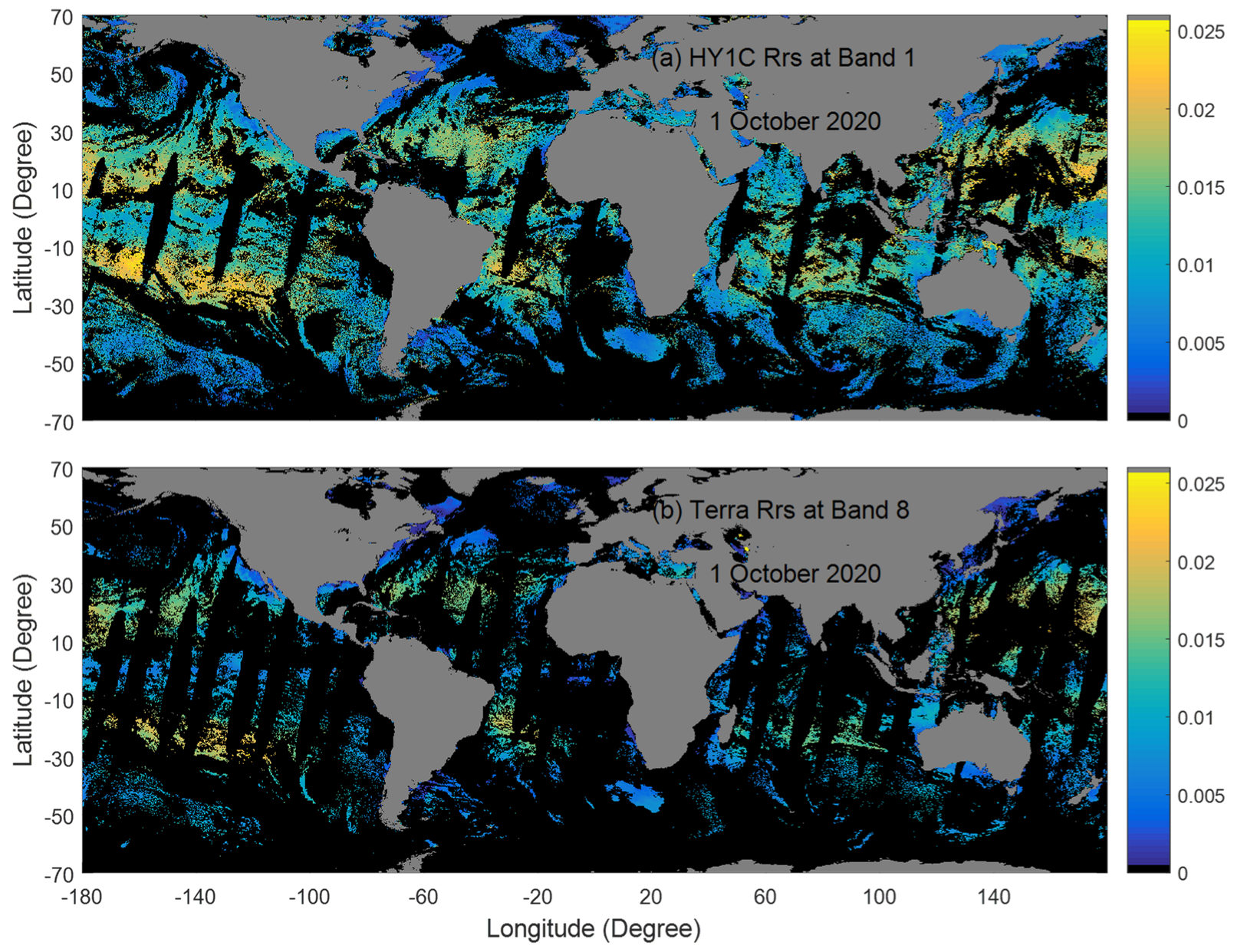
A total of 182 L1B files on 1 October 2020 were processed to obtain Rrs by the LRSAC, and then the data at Band 1 were projected into a global image with a spatial resolution of 4 by 4 km, as shown in Figure 4a, together with an image at Band 8 of MODIS/Terra on the same day in Figure 4b. The two satellites observe the ocean at around 10:30 local time, reducing the differences of the reflectance due to the time window.
A first look at the two images in Figure 4 reveals the large difference in the valid pixels, with 32.3% for HY-1C, almost three times that for Terra (11.9%). This difference is caused by several factors. One factor is the swath of COCTS wider than 2900 km in Equatorial regions, completely covering the whole global ocean with one day revisiting period. Meanwhile, the viewing zenith angles become large at the borders of the scan lines, with the largest value being higher than 72°. The capability of the LRSAC is important in processing the data with the condition of high viewing zenith angles. The second factor is the capability of the LRSAC in the presence of a high aerosol optical depth [5]. The third factor is the performance of the LRSAC in the high-latitude regions with large values of solar zenith angles [5]. The fourth factor is the performance of the LRSAC in recovering some contaminated pixels by removing the effect of the glint reflectance with values lower than 0.03 sr−1. The comparisons exhibit that the gaps in the COCTS/HY-1C images are significantly reduced and improve the visibility of ocean dynamic features.
The consistency of the Rrs imagery between HY-1C and Terra was evaluated by the matchups that were established from the two images when both pixels were valid on the same location, as shown in Figure 5.
It is clear that most dots of matchups fall around the 1:1 lines for all six bands, and the concentrated clusters of pairs locate at the line in six subfigures. The patterns of Figure 5 indicate that the Rrs of HY-1C agree well with those from the Terra, and the biases between HY-1C and Terra are relatively small. All pairs are used to compute MPD and MAD, as shown in Table 4, but some pairs with an RE higher than 100% are excluded from the computations of other metrics.
From Table 4, it can be seen that the MRE values vary from 3.35% at Band 1 to 13.84% at Band 5, with a mean of 10.94%. The MPD values vary around 9%, except for Band 6 (62.71%). The MAE values range between 19.48% and 24.73%, with a mean of 21.38%. The MAD values vary around 16%, except for Band 6 (93.09%). The RMS values vary from 0.0015 sr−1 (Band 6) to 0.0062 sr−1 (Band 1). Comparing the RMS values with those of MOBY in Table 1, the values are much larger, by about 3 times at Band 1 and 40 times at Band 6. The coefficients of determination are relatively high, with values from 0.66 (Band 4) to 0.93 (Band 6).
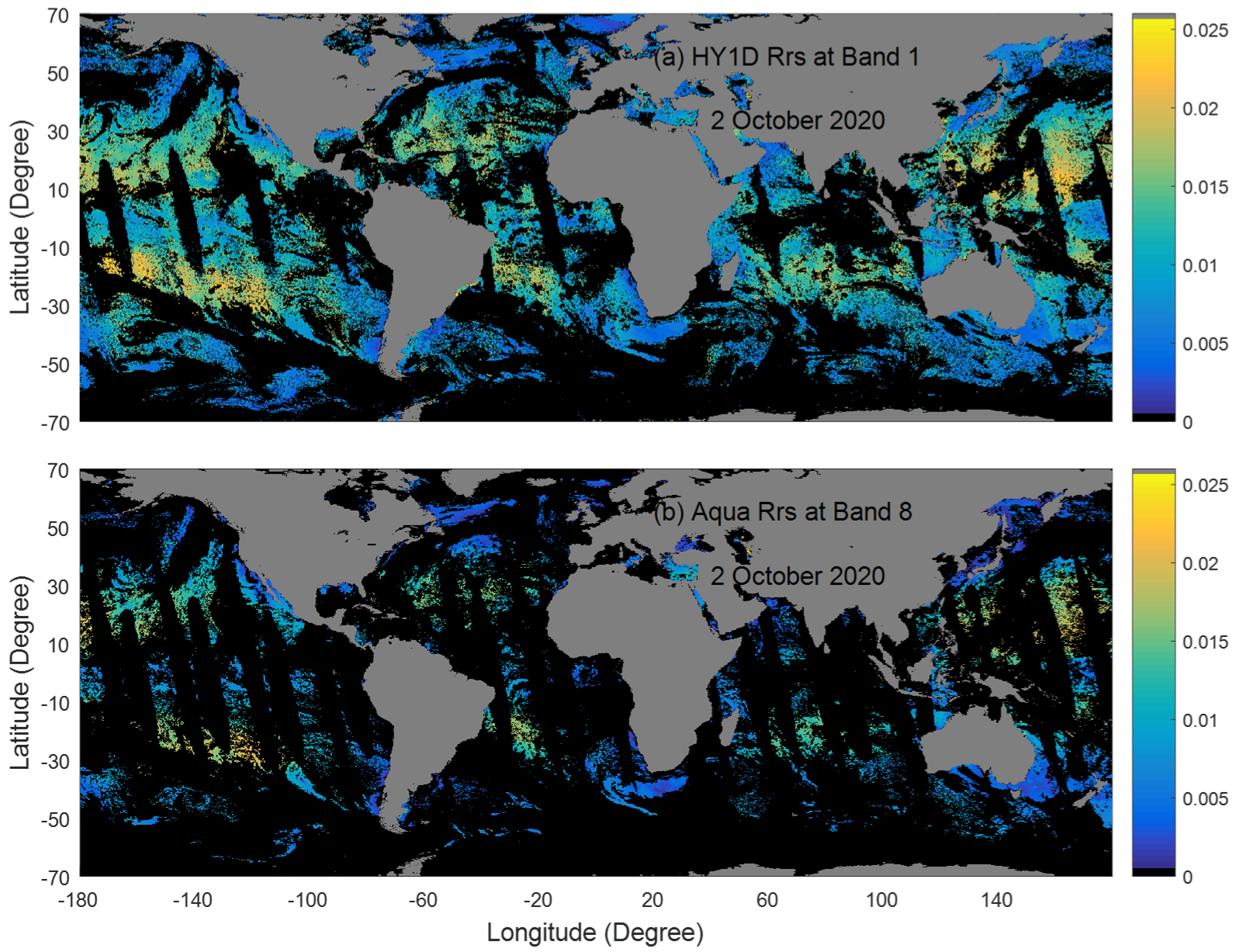
The HY-1D is the afternoon satellite with an overpass time at the Equator around 13:30 P.M. local time, which is close to that of the Aqua. It obviously reduces the differences due to the time window and the comparison of the two images at the blue band is shown in Figure 6. Clouds are the main cause reducing the number of valid pixels, and clouds are flagged by the values of Rrs at the two NIR bands (>0.005 sr−1) for oceanic waters.
As expected, the spatial distributions of the Rrs image from COCTS/HY-1D are similar to those from MODIS/Terra. The areas with high values of HY-1D are consistent with those of Terra, mainly distributed around the middle latitude regions. The main difference of the two images is the number of valid pixels, which is 32.6% of HY-1D, much higher than that of Aqua (11.9%). The smaller gaps in the HY-1D image also benefit from the performance of the LRSAC in the AC procedure under the conditions of high viewing zenith angles, a high solar zenith angle and a high aerosol optical depth. The values of Aqua were used to evaluate the consistency of Rrs of HY-1D, and the matchups were established from both valid pixels, as shown in Figure 7.
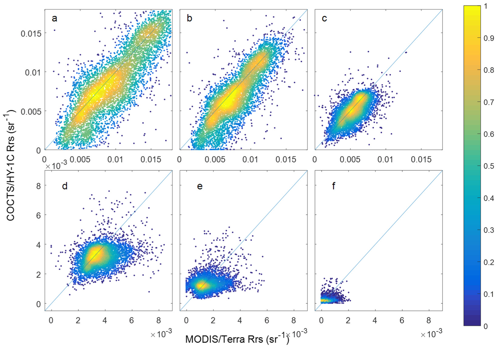
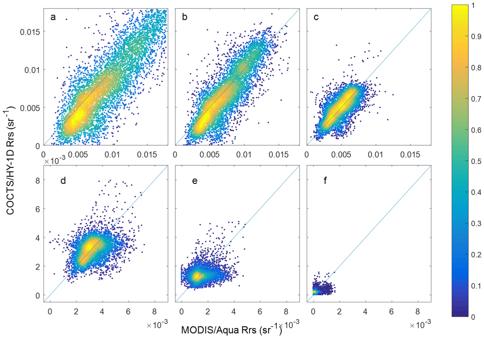
The scatterplots of the COCTS/HY-1D versus the MODIS/Aqua at six bands show that most dots are distributed around the 1:1 line. The patterns in Figure 7 are similar to those in Figure 5, indicating that the values of the Rrs imagery from HY-1D are comparable with those of Aqua. To evaluate the consistency of the satellite-retrieved products of HY-1D, the matchups were established from the same valid pixels of the two images, and the values of Aqua are taken as the truth data. Similarly, all pairs are used to compute MPD and MAD, but some pairs with an RE higher than 100% are excluded from the computations of other metrics in Table 5.
From Table 5, the MRE values vary from 11.07% at Band 1 to 14.74% at Band 4, with a mean of 13.31%. The MAE values range between 19.45% and 23.36%, with a mean of 21.46%. The MPD values vary about 10% and the MAD values vary about 20%. The RMS values decrease from 0.0069 sr−1 (Band 1) to 0.0015 sr−1 (Band 6). The coefficients of determination are also relatively high, from 0.71 to 0.94. These values are close to those in Table 3 at corresponding bands, indicating that the consistency of Rrs products between HY-1C and Terra is similar to that between HY-1D and Aqua.
3.3. The Comparison of 8-Day Composite Products
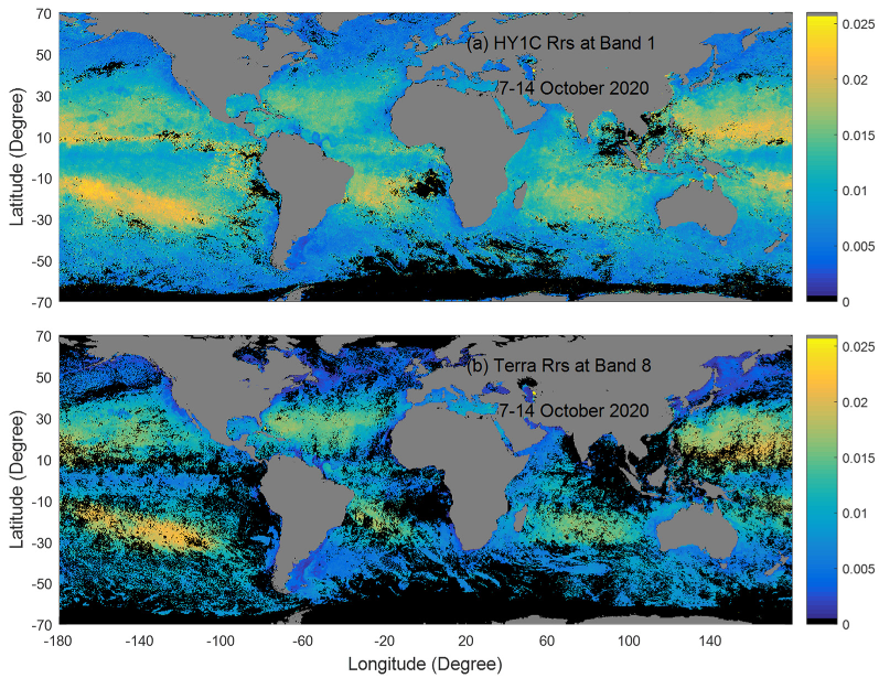
Due to the low coverage of valid pixels in the global daily Rrs images, the 8-day composite imagery can significantly reduce the gaps which are provided on the website as a kind of standard product. The 8-day image, produced from the Rrs images of COCTS/HY-1C during the period of 7 to 15 October 2020, is shown in Figure 8a, together with that from Terra in the same time period in Figure 8b. It is obvious that there are still many gaps that are empty for the composite images, such as some areas due to high AOD distributions over the oceans caused by the Saharan dust, which can last for a period of time [37].
The numbers of valid pixels in the two composite images significantly increase by 83.9% for HY-1C and by 52.9% for Terra. The increase in valid pixels improves the usability of the large-scale ocean features and helps reveal the spatial structures of the dynamic ocean in the composite images [23]. High values are distributed in the Pacific in the latitude range of 10–30 degrees. These regions are consistent with the five gyres, with the lowest primary productivity referred to as “ocean deserts” [38].
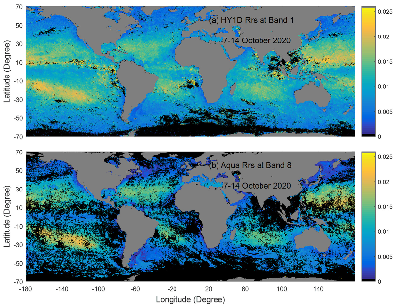
Comparing the two images in Figure 8, the differences in valid pixels are significant. Only 16.1% of the regions of HY-1C are covered with invalid pixels, while the number reaches to 47.1% for Terra. From the spatial distribution, most of the invalid pixels in the Equatorial regions are mainly due to the presence of a high AOD, and the numbers of valid pixels between the images are large. For the region with latitudes between −50 and 50 degrees, the percentage of invalid pixels of HY-1C is only 6.9%, which is much lower than that of Terra (37.7%). The invalid pixels around the two poles are mainly due to the weak sunlight under high solar zenith angles, and the differences between the two images are also significant. The percentage of invalid pixels of HY-1C in the regions with latitudes higher than 50 degrees is 5.9%, which is much lower than that of Terra (40.2%). Similarly, a comparison of the 8-day composite images between HY-1D and Aqua is shown in Figure 9.
The numbers of valid pixels are also significantly different between the HY-1D images (85.4%) and the Aqua image (50.9%). Similarly, the percentage of invalid pixels of HY-1D is about 7.8%, which is much lower than that of Terra (55.3%) for the region with latitudes between −50 and 50 degrees. The percentage in the regions with latitudes higher than 50 degrees is 5.7%, which is much lower than that of Terra (59.2%). Therefore, the LRSAC model can greatly increase the coverage of valid pixels of the Rrs imagery from HY-1C/1D.
4. Discussion
4.1. The Removal of the Sun Glint Contamination
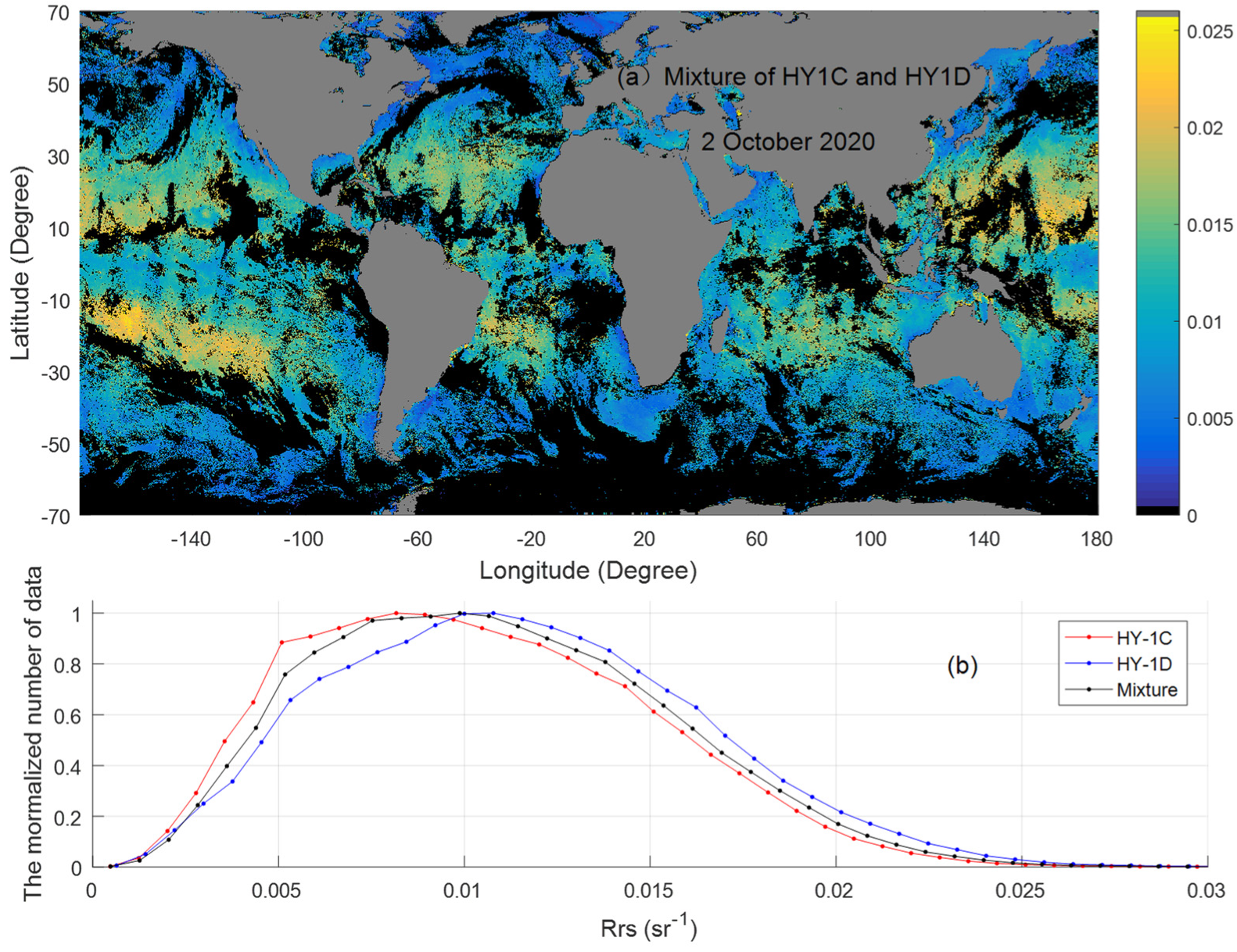
The presence of sun glint will produce gaps in the imagery of HY-1C/1D. Can the composite image of HY-1C and HY-1D on the same day significantly reduce the coverage of the gaps due to the contamination of sun glint? To demonstrate this question, a merged image is produced from the mean of the two global daily images of HY-1C/1D on 2 October and is shown in Figure 10a, together with the comparison of the data distribution of the three images in Figure 10b.
It is obvious that most gaps, due to the contamination of sun glint in the images of HY-1C and HY-1D, can be filled by valid pixels in the merged image of Figure 10a. The coverage of sun glint occupies 6.6% in the global daily image of HY-1C on 2 October 2020, and it is 7.6% in the HY-1D image on the same day using the threshold of glint reflectance higher than 0.03 sr−1. The coverage of glint contamination reduces to 0.7% in the merged image of Figure 10a. In fact, the coverage of gaps strongly depends on the threshold for flagging the sun glint contamination. When the threshold becomes 0.005 sr−1, the coverage of the glint flag reaches 24.8% for HY-1C and 27.2% for HY-1D. The coverage of the gaps in the merged image is also significantly reduced but still holds a relatively large value (8.8%). It demonstrates that a suitable threshold for flagging the sun glint contamination needs be carefully evaluated from the balance between the coverage of glint gaps and the data quality of the imagery. However, the merged image of HY-1C and HY-1D on the same day can significantly reduce the coverage of glint gaps.
When the images of HY-1C and HY-1D on the same day are merged into one image, the consistency of the two images is critical to affecting the data quality of the composite image. To demonstrate this, Figure 10b shows that the distributions between HY-1C and HY-1D at Band 1 are similar to each other, but the value with the largest histogram is different, with 0.011 sr−1 for HY-1D and 0.008 sr−1 for HY-1C. As the merged image was produced from the mean values of the two images, it can reduce the differences in Rrs between HY-1C and HY-1D. The images on other days were also tested by the same method and showed similar results.
4.2. The 3-Day Composite Images
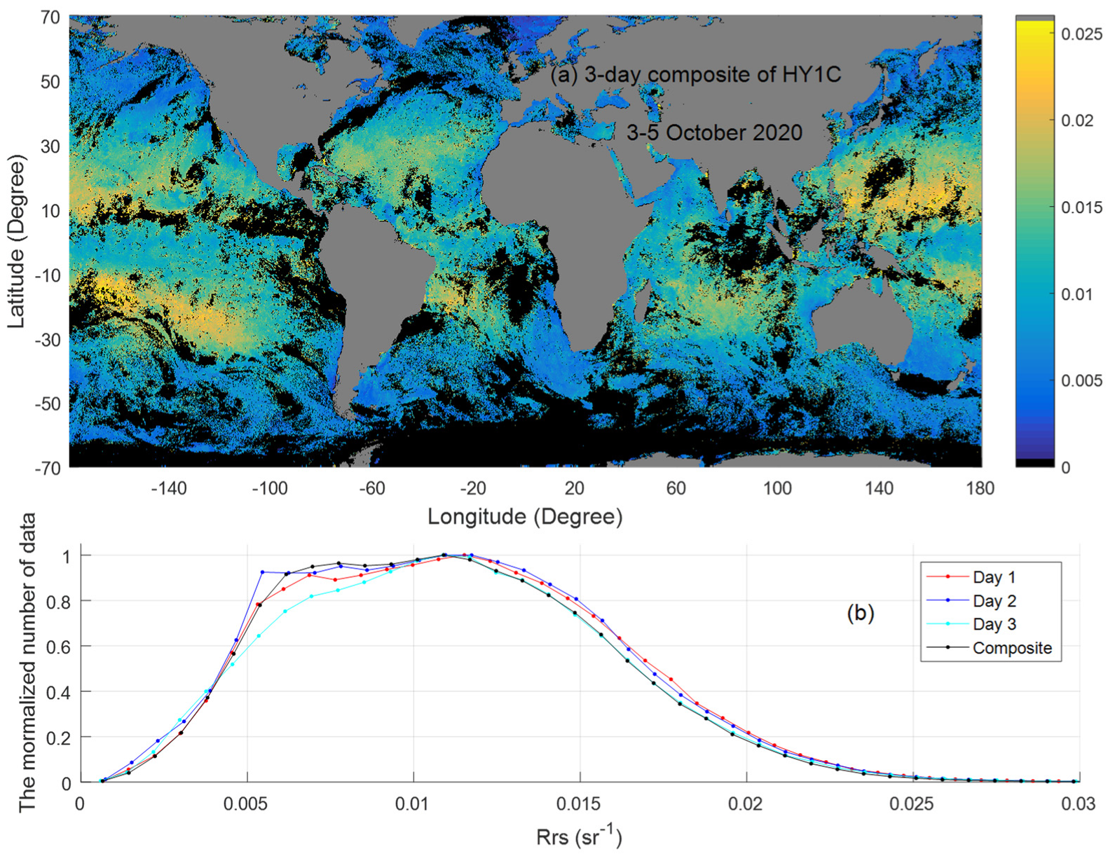
The 8-day composite imagery can significantly reduce the coverage of gaps, but it may introduce uncertainty due to the temporal variations in the reflectance during a period of 8 days. How can one balance the coverage of gaps and the uncertainty of the time period? To demonstrate this question, a 3-day composite image is merged from the images during 3–5 October 2020, as shown in Figure 11, together with the data distribution comparison of the three images.
From the image of HY-1C in Figure 11a, all gaps, due to the contamination of sun glint, have almost been removed, together with some gaps due to clouds and other factors. The coverage of valid pixels in the 3-day image of HY-1C reaches 63.5%, which is higher than that of the 8-day composite image of Terra or Aqua. Similarly, the percentage of valid pixels in the 3-day image of HY-1D is 65.6%, and that of the 3-day image merged from HY-1C and HY-1D reaches 76.1%. The comparison of the data distributions between the merged image and the images in the three days shows that the consistency is kept well among these products. A dataset of the 3-day composite imagery, with a coverage of about 70% of valid pixels exhibiting most of the ocean spatial patterns, provides another kind of product for some applications which are sensible for the time period.
4.3. The Spectral Variations over the Ocean Dynamic Features
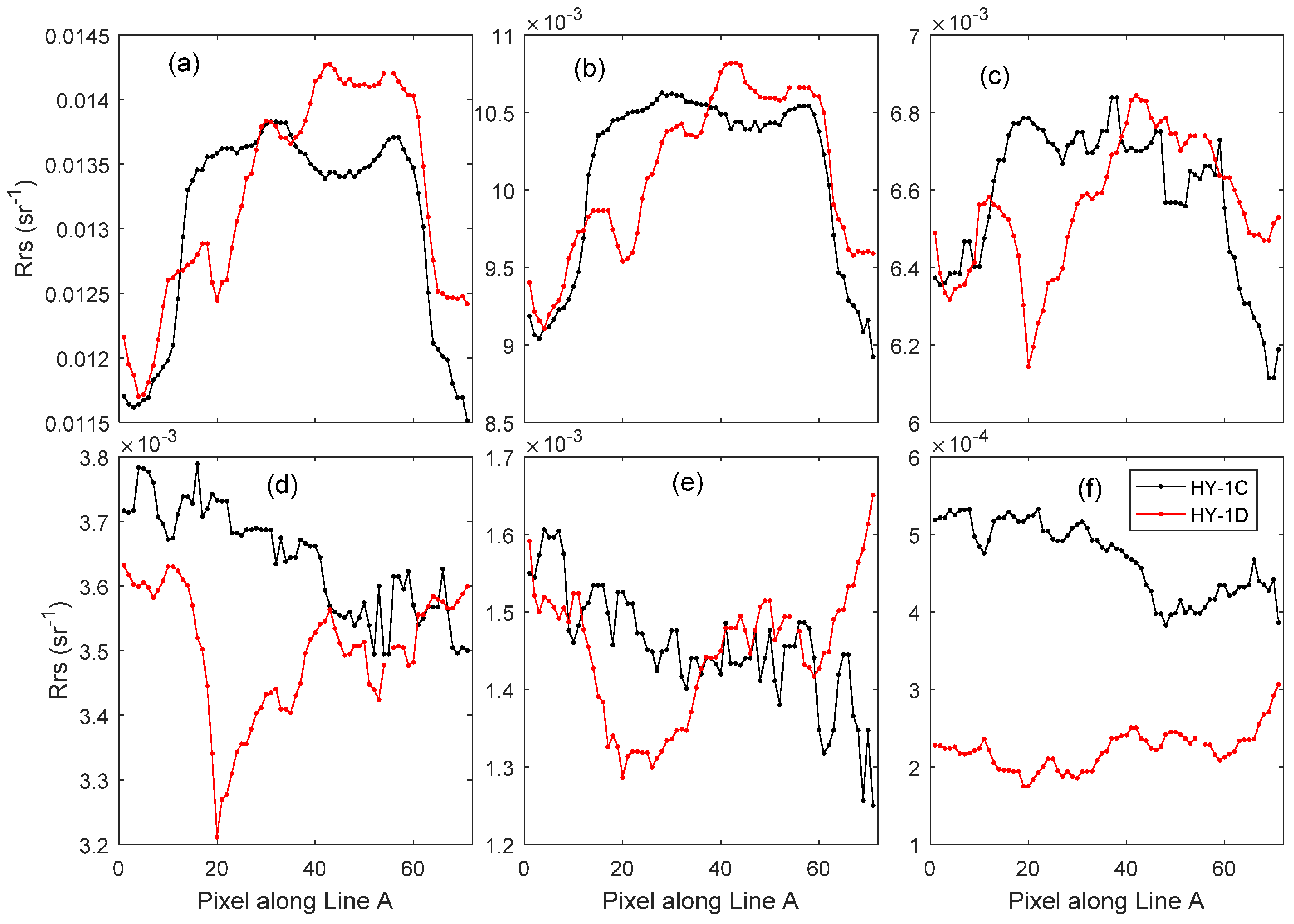
There are some ocean dynamic features distributed around the MOBY site in the images of Figure 1, demonstrating that the sensitivity of the Rrs of HY-1C/1D is high enough to identify small spectral variations of ocean fronts. To understand how the values of different bands change across the fronts, the Rrs values along Line A in Figure 1 are extracted and shown in Figure 12.
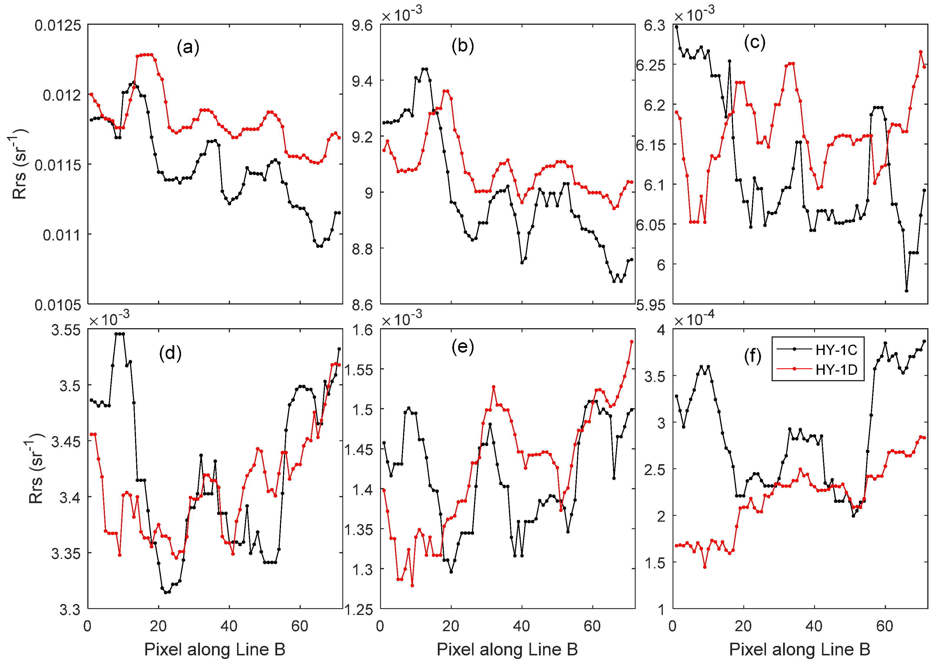
It is obvious that the spatial shapes of Rrs at different bands change largely across the fronts. The spectral structures of HY-1C at Bands 1–3 are similar to each other, and the spatial patterns are consistent with features across Line A in Figure 1, but they are different from those of Bands 4–6. This demonstrates that the Rrs values at different bands exhibit large differences across the same ocean features. The spectral patterns of HY-1D are similar to those of HY-1C, with some differences at the corresponding bands, indicating the structures of the ocean fronts change in the time period of 3 h on the assumption of the same spectral responses of HY-1C and HY-1D. The spatial patterns of Band 6 are relatively stable, but, actually, the values vary largely. The mean value of HY-1C is 4.71 × 10⁻⁴ sr−1, which is one times higher than that of HY-1D (2.22 × 10⁻⁴ sr−1). The MAE will reach 116.4% when the values of HY-1D are taken as the truth values. This demonstrates that an uncertainty of the evaluation of the satellite-retrieved products may be introduced due to the temporal variations in the ocean within 3 h. In comparison, the spectral values at six bands across Line B are shown in Figure 13.
From Figure 1, it can be seen that the spatial variations in the ocean dynamic features across Line B are much weaker than those across Line A. However, the patterns in Figure 13 demonstrate that the sensitivity of HY-1C/1D is high enough to identify these small spectral variations. The patterns of Rrs at Band 1 of HY-1C and HY-1D exhibit four small peaks across Line B, but these peaks show different spatial structures among six bands. The mean values of HY-1C are close to those of HY-1D, but the values on the pixel scale vary relatively largely. This demonstrates that a large uncertainty of the evaluation may be introduced due to the spatial variations in the ocean on the pixel scale within 3 h. However, it is still difficult to estimate how many percentages of these variations are caused by the ocean dynamics during a short time period and by the spectral responses of different satellite sensors, which may be understood from more observations of different satellites on the same day in the future.
5. Conclusions
The comparisons of the Rrs imagery between COCTS on the HY-1C/1D and MODIS on the Terra/Aqua show that the global daily and 8-day composite Rrs products of COCTS are consistent with those of MODIS at six bands, with most matchups distributed around the 1:1 lines. The evaluations of Rrs from COCTS using MOBY measurements show that the accuracy of HY-1C/1D products is good enough for them to be used as a kind of standard product for the international ocean color community.
The coverage of gaps in the global daily Rrs imagery of HY-1C/1D is significantly reduced, with 32.2% of valid pixels for HY-1C and 32.6% for HY-1D, about 3 times of those for Terra/Aqua. The increase in the valid pixels benefits from the wide swath of COCTS, which is wider than 2900 km at the Equatorial regions. In fact, the removal of gaps in the imagery of HY-1C/1D benefits from the ability of the LRSAC model to retrieve Rrs in the presence of high viewing zenith angles, high solar zenith angles and high aerosol optical depths.
The merged image of HY-1C and HY-1D on the same day can significantly reduce the coverage of gaps due to the contamination of sun glint. It needs to be carefully evaluated in selecting a suitable threshold for flagging the sun glint contamination from the balance between the coverage of glint contamination and the data quality of the imagery. Many gaps of sun glint can also be removed in the 3-day composite imagery of COCTS, with the number of valid pixels higher than that of the 8-day composite of MODIS. The 3-day imagery of HY-1C/1D improves the visibility of ocean dynamic features and reduces the temporal variations during a time period, providing another kind of product for some applications which are sensible for the time period.
The pseudo images around the MOBY site show that the sensitivity of HY-1C/1D is high enough to identify the ocean dynamic features. The spatial distributions of the features are consistent with the shapes across the ocean fronts, but the shapes of peaks vary largely among different bands. The shapes of HY-1C are similar to those of HY-1D, with many differences mainly due to the temporal variations in the ocean features within 3 h. This short time period causes the magnitudes of HY-1C across the fronts to vary with those of HY-1D on the pixel scale, although they are close to each other in a whole. The temporal variations in the reflectance obviously increase the uncertainty of the Rrs products in the evaluation procedure, especially a small variation at Band 6, which easily led to a large RE value due to the small magnitudes of Rrs.
Author Contributions
Conceptualization, Z.M. and Y.Z.; methodology, Z.M.; software, Q.Z.; validation, B.T. and J.C.; formal analysis, Z.H.; investigation, B.T.; resources, Q.Z.; data curation, H.H.; writing—original draft preparation, Z.M.; writing—review and editing, Y.Z.; visualization, Z.H.; supervision, J.C.; project administration, H.H.; funding acquisition, H.H. All authors have read and agreed to the published version of the manuscript.
Funding
This research was funded by the National Science Foundation of China (61991454), the Major Project of High-Resolution Earth Observation Systems of National Science and Technology (05-Y30B01-9001-19/20-2) and the National Key Research and Development Program of China (2016YFC1400901).
Data Availability Statement
The remote sensing data of COCTS on HY-1C/1D are available at https://osdds.nsoas.org.cn/ (accessed on 1 January 2022).
Acknowledgments
We would like to thank the organizations that provided in situ measurements and satellite remote sensing data.
Conflicts of Interest
The authors declare no conflict of interest. The funders had no role in the design of the study; in the collection, analyses or interpretation of the data; in the writing of the manuscript or in the decision to publish the results.
References
- Mao, Z.; Chen, P.; Tao, B.; Ding, J.; Liu, J.; Chen, J.; Hao, Z.; Zhu, Q.; Huang, H. A Radiometric Calibration Scheme for COCTS/HY-1C Based on Image Simulation from the Standard Remote-Sensing Reflectance. IEEE Trans. Geosci. Remote Sens. 2021, 60, 1–9. [Google Scholar] [CrossRef]
- HY-1C/D-EoPortal Directory-Satellite Missions. Available online: https://directory.eoportal.org/web/eoportal/satellite-missions/hy-1c-1d (accessed on 1 January 2021).
- Cai, L.; Zhou, M.; Liu, J.; Tang, D.; Zuo, J. HY-1C Observations of the Impacts of Islands on Suspended Sediment Distribution in Zhoushan Coastal Waters, China. Remote Sens. 2020, 12, 1766. [Google Scholar] [CrossRef]
- Chen, X.-Y.; Zhang, J.; Tong, C.; Liu, R.-J.; Mu, B.; Ding, J. Retrieval Algorithm of Chlorophyll-a Concentration in Turbid Waters from Satellite HY-1C Coastal Zone Imager Data. J. Coast. Res. 2019, 90, 146–155. [Google Scholar] [CrossRef]
- Mao, Z.; Tao, B.; Chen, J.; Chen, P.; Hao, Z.; Zhu, Q.; Huang, H. A Layer Removal Scheme for Atmospheric Correction of Satellite Ocean Color Data in Coastal Regions. IEEE Trans. Geo. Remote Sens. 2021, 59, 1382–1391. [Google Scholar] [CrossRef]
- Warren, M.A.; Simis, S.G.H.; Martinez-Vicente, V.; Poser, K.; Bresciani, M.; Alikas, K.; Spyrakos, E.; Giardino, C.; Ansper, A. Assessment of atmospheric correction algorithms for the Sentinel-2A Multi-Spectral Imager over coastal and inland waters. Remote Sens. Environ. 2019, 225, 267–289. [Google Scholar] [CrossRef]
- Doxani, G.; Vermote, E.; Roger, J.; Gascon, F.; Adriaensen, S.; Frantz, D.; Hagolle, O.; Hollstein, A.; Kirches, G. Atmospheric Correction Inter-Comparison Exercise. Remote Sens. 2018, 10, 352. [Google Scholar] [CrossRef] [Green Version]
- Wei, J.; Lee, Z.; Garcia, R.; Zoffoli, L.; Armstrong, R.A.; Shang, Z.; Sheldon, P.; Chen, R.F. An assessment of Landsat-8 atmospheric correction schemes and remote sensing reflectance products in coral reefs and coastal turbid waters. Remote Sens. Environ. 2018, 215, 18–32. [Google Scholar] [CrossRef]
- Ilori, C.; Pahlevan, N.; Knudby, A. Analyzing Performances of Different Atmospheric Correction Techniques for Landsat 8: Application for Coastal Remote Sensing. Remote Sens. 2019, 11, 469. [Google Scholar] [CrossRef] [Green Version]
- Bailey, S.W.; Franz, B.A.; Werdell, P.J. Estimation of Near-Infrared Water-Leaving Reflectance for Satellite Ocean Color Data Processing. Opt. Express 2010, 18, 7521–7527. [Google Scholar] [CrossRef]
- Oo, M.; Vargas, M.; Gilerson, A.; Gross, B.; Moshary, F.; Ahmed, S. Improving Atmospheric Correction for Highly Productive Coastal Waters Using the Short Wave Infrared Retrieval Algorithm with Water-Leaving Reflectance Constraints at 412 Nm. Appl. Opt. 2008, 47, 3846–3859. [Google Scholar] [CrossRef]
- Mao, Z.; Pan, D.; He, X.; Chen, J.; Tao, B.; Chen, P.; Hao, Z.; Bai, Y.; Zhu, Q.; Huang, H. A Unified Algorithm for the Atmospheric Correction of Satellite Remote Sensing Data over Land and Ocean. Remote Sens. 2016, 8, 536. [Google Scholar] [CrossRef] [Green Version]
- Wang, M.; Jiang, L. Atmospheric Correction Using the Information from the Short Blue Band. IEEE Trans. Geo. Remote Sens. 2018, 56, 6224–6237. [Google Scholar] [CrossRef]
- Jiang, L.; Wang, M. Improved Near-Infrared Ocean Reflectance Correction Algorithm for Satellite Ocean Color Data Processing. Opt. Express 2014, 22, 21657–21678. [Google Scholar] [CrossRef] [PubMed]
- Singh, R.K.; Shanmugam, P.; He, X.; Schroeder, T. UV-NIR Approach with Non-Zero Water-Leaving Radiance Approximation for Atmospheric Correction of Satellite Imagery in Inland and Coastal Zones. Opt. Express 2019, 27, A1118–A1145. [Google Scholar] [CrossRef]
- Zhang, M.; Hu, C.; Barnes, B.B. Performance of POLYMER Atmospheric Correction of Ocean Color Imagery in the Presence of Absorbing Aerosols. IEEE Trans. Geo. Remote Sens. 2019, 57, 6666–6674. [Google Scholar] [CrossRef]
- Mao, Z.; Tao, B.; Chen, P.; Chen, J.; Hao, Z.; Zhu, Q.; Huang, H. Atmospheric Correction of Satellite Ocean Color Remote Sensing in the Presence of High Aerosol Loads. Remote Sens. 2019, 12, 31. [Google Scholar] [CrossRef] [Green Version]
- Goyens, C.; Jamet, C.; Schroeder, T. Evaluation of Four Atmospheric Correction Algorithms for MODIS-Aqua Images over Contrasted Coastal Waters. Remote Sens. Environ. 2013, 131, 63–75. [Google Scholar] [CrossRef]
- Carswell, T.; Costa, M.; Young, E.; Komick, N.; Gower, J.; Sweeting, R. Evaluation of MODIS-Aqua Atmospheric Correction and Chlorophyll Products of Western North American Coastal Waters Based on 13 Years of Data. Remote Sens. 2017, 9, 1063. [Google Scholar] [CrossRef] [Green Version]
- Wang, M.; Son, S.; Shi, W. Evaluation of MODIS SWIR and NIR-SWIR Atmospheric Correction Algorithms Using SeaBASS Data. Remote Sens. Environ. 2009, 113, 635–644. [Google Scholar] [CrossRef]
- Wang, M.; Wei, S. Estimation of Ocean Contribution at the MODIS Near-Infrared Wavelengths along the East Coast of the U.S.: Two Case Studies. Geo. Res. Lett. 2005, 32, L13606. [Google Scholar] [CrossRef]
- Mao, Z.; Mao, Z.; Jamet, C.; Linderman, M.; Wang, Y.; Chen, X. Seasonal Cycles of Phytoplankton Expressed by Sine Equations Using the Daily Climatology from Satellite-Retrieved Chlorophyll-a Concentration (1997–2019) Over Global Ocean. Remote Sens. 2020, 12, 2662. [Google Scholar] [CrossRef]
- Liu, X.; Wang, M. Filling the Gaps of Missing Data in the Merged VIIRS SNPP/NOAA-20 Ocean Color Product Using the DINEOF Method. Remote Sens. 2019, 11, 178. [Google Scholar] [CrossRef] [Green Version]
- Liu, J.; Li, Z.; Qiao, Y.; Liu, Y.; Zhang, Y. A New Method for Cross-Calibration of Two Satellite Sensors. Int. J. Remote Sens. 2004, 25, 5267–5281. [Google Scholar] [CrossRef]
- Chander, G.; Xiong, X.; Choi, T.; Angal, A. Monitoring On-Orbit Calibration Stability of the Terra MODIS and Landsat 7 ETM+ Sensors Using Pseudo-Invariant Test Sites. Remote Sens. Environ. 2010, 114, 925–939. [Google Scholar] [CrossRef]
- Sayer, A.M.; Hsu, N.C.; Bettenhausen, C.; Holz, R.E.; Lee, J.; Quinn, G.; Veglio, P. Cross-Calibration of S-NPP VIIRS Moderate-Resolution Reflective Solar Bands against MODIS Aqua over Dark Water Scenes. Atmos. Meas. Tech. 2017, 10, 1425–1444. [Google Scholar] [CrossRef] [Green Version]
- Chen, J.; He, X.; Liu, Z.; Xu, N.; Ma, L.; Xing, Q.; Hu, X.; Pan, D. An Approach to Cross-Calibrating Multi-Mission Satellite Data for the Open Ocean. Remote Sens. Environ. 2020, 246, 111895. [Google Scholar] [CrossRef]
- Gordon, H.R.; Wang, M. Retrieval of Water-Leaving Radiance and Aerosol Optical Thickness over the Oceans with SeaWiFS: A Preliminary Algorithm. Appl. Opt. 1994, 33, 443–452. [Google Scholar] [CrossRef]
- Shi, W.; Wang, M. Detection of Turbid Waters and Absorbing Aerosols for the MODIS Ocean Color Data Processing. Remote Sens. Environ. 2007, 110, 149–161. [Google Scholar] [CrossRef]
- Brown, S.W.; Flora, S.J.; Feinholz, M.E.; Yarbrough, M.A.; Houlihan, T.; Peters, D.; Kim, Y.S.; Mueller, J.L.; Johnson, B.C.; Clark, D.K. The Marine Optical Buoy (MOBY) Radiometric Calibration and Uncertainty Budget for Ocean Color Satellite Sensor Vicarious Calibration. In Sensors, Systems, and Next-Generation Satellites XI; Habib, S., Meynart, R., Neeck, S.P., Shimoda, H., Eds.; SPIE: Bellingham, WA, USA, 2007; Volume 6744, pp. 433–444. [Google Scholar]
- Lacis, A.A.; Hansen, J.E. A Parameterization for the Absorption of Solar Radiation in the Earth’s Atmosphere. J. Atmos. Sci. 1974, 31, 118–133. [Google Scholar] [CrossRef]
- Kotchenova, S.Y.; Vermote, E.F.; Matarrese, R.; Klemm, F.J., Jr. Validation of a Vector Version of the 6S Radiative Transfer Code for Atmospheric Correction of Satellite Data Part I: Path Radiance. Appl. Opt. 2006, 45, 6762–6774. [Google Scholar] [CrossRef]
- Kotchenova, S.Y.; Vermote, E.F. Validation of a Vector Version of the 6S Radiative Transfer Code for Atmospheric Correction of Satellite Data Part II Homogeneous Lambertian and Anisotropic Surfaces. Appl. Opt. 2007, 46, 4455–4464. [Google Scholar] [CrossRef] [PubMed] [Green Version]
- Gordon, H.R.; Wang, M. Surface-Roughness Considerations for Atmospheric Correction of Ocean Color Sensors. I: The Rayleigh-Scattering Component. Appl. Opt. 1992, 31, 4247–4260. [Google Scholar] [CrossRef] [PubMed]
- Cox, C.; Munk, W. Measurement of the Roughness of the Sea Surface from Photographs of the Sun’s Glitter. J. Opt. Soc. Am. 1954, 44, 838–850. [Google Scholar] [CrossRef]
- Frouin, R.; Schwindling, M.; Deschamps, P.-Y. Spectral Reflectance of Sea Foam in the Visible and Near-Infrared: In Situ Measurements and Remote Sensing Implications. J. Geophy. Res. Oceans 1996, 101, 14361–14371. [Google Scholar] [CrossRef]
- Moulin, C.; Gordon, H.R.; Banzon, V.F.; Evans, R.H. Assessment of Saharan Dust Absorption in the Visible from SeaWiFS Imagery. J. Geophy. Res. Atmos. 2001, 106, 18239–18249. [Google Scholar] [CrossRef]
- Jena, B.; Swain, D.; Avinash, K. Investigation of the biophysical processes over the oligotrophic waters of South Indian Ocean subtropical gyre, triggered by cyclone Edzani. Int. J. Appl. Earth Obs. Geo. 2012, 18, 49–56. [Google Scholar] [CrossRef]
Figure 1.
The composite Rrs images of Bands 1–3 from the MODIS on 6 October 2020 with Terra (a) and Aqua (b); those from COCTS on HY-1C (c) and HY-1D (d), where the red cross marks the position of the MOBY site and two blue lines (A and B) are used to demonstrate the structures of spectra along the lines in Figures 12 and 13; the spectral Rrs comparison of the in situ measurements at the MOBY site (red line) and the satellite-retrieved images (green line) for HY-1C (e) and HY-1D (f).

Figure 2.
The comparison of Rrs matchups between COCTS/HY-1C and MOBY measurements on the same day, with the density of dots indicated by different colors. Subfigures (a–f) represent the values at Bands 1–6.
Figure 2.
The comparison of Rrs matchups between COCTS/HY-1C and MOBY measurements on the same day, with the density of dots indicated by different colors. Subfigures (a–f) represent the values at Bands 1–6.

Figure 3.
The comparison of Rrs between the COCTS/HY-1D and MOBY measurements on the same day. Subfigures (a–f) represent the values in Bands 1–6, respectively.
Figure 3.
The comparison of Rrs between the COCTS/HY-1D and MOBY measurements on the same day. Subfigures (a–f) represent the values in Bands 1–6, respectively.

Figure 4.
The comparison of the global daily Rrs image on 1 October 2020 with (a) COCTS/HY-1C at Band 1 and (b) MODIS/Terra at Band 8. The magnitudes of image pixels are indicated by the color bar with the unit of sr−1. Invalid pixels are masked black and land grey.
Figure 4.
The comparison of the global daily Rrs image on 1 October 2020 with (a) COCTS/HY-1C at Band 1 and (b) MODIS/Terra at Band 8. The magnitudes of image pixels are indicated by the color bar with the unit of sr−1. Invalid pixels are masked black and land grey.

Figure 5.
Evaluation of the consistency of the daily global Rrs imagery between COCTS/HY-1C and MODIS/Terra on 2 October 2020 at six bands (a–f).
Figure 5.
Evaluation of the consistency of the daily global Rrs imagery between COCTS/HY-1C and MODIS/Terra on 2 October 2020 at six bands (a–f).

Figure 6.
The comparison of the global daily Rrs image on 2 October 2020 with (a) COCTS/HY-1D at Band 1 and (b) MODIS/Aqua at Band 8. The magnitudes of image pixels are indicated by the color bar with the unit of sr−1. Invalid pixels are masked black and land grey.
Figure 6.
The comparison of the global daily Rrs image on 2 October 2020 with (a) COCTS/HY-1D at Band 1 and (b) MODIS/Aqua at Band 8. The magnitudes of image pixels are indicated by the color bar with the unit of sr−1. Invalid pixels are masked black and land grey.

Figure 7.
Evaluation of the consistency of the daily global Rrs imagery between C CTS/HY-1D and MODIS/Aqua on 2 October 2020 at six bands (a–f).
Figure 7.
Evaluation of the consistency of the daily global Rrs imagery between C CTS/HY-1D and MODIS/Aqua on 2 October 2020 at six bands (a–f).

Figure 8.
The comparison of the 8-day composite Rrs image between COCTS/HY-1C at Band 1 (a) and MODIS/Terra at Band 8 (b). Both are produced from the global daily images during the period of 7 to 14 October 2020. The magnitudes of image pixels are indicated by the color bar with the unit of sr−1. Invalid pixels are masked black and land grey.

Figure 9.
The comparison of the 8-day composite Rrs image between COCTS/HY-1D at Band 1 (a) and MODIS/Aqua at Band 8 (b). Both are produced from the global daily images during the period of 7 to 14 October 2020. The magnitudes of image pixels are indicated by the color bar with the unit of sr−1. Invalid pixels are masked black and land grey.

Figure 10.
(a) The composite Rrs image at Band 1, merged from the two images of HY-1C and HY-1D on 2 October 2020, and (b) the comparison of the Rrs data distribution of the three images, normalized to the maximum of 1.
Figure 10.
(a) The composite Rrs image at Band 1, merged from the two images of HY-1C and HY-1D on 2 October 2020, and (b) the comparison of the Rrs data distribution of the three images, normalized to the maximum of 1.

Figure 11.
(a) The 3-day composite Rrs image at Band 1, merged from HY-1C during 3–5 October 2020, and (b) the comparison of the Rrs data distribution of the images.
Figure 11.
(a) The 3-day composite Rrs image at Band 1, merged from HY-1C during 3–5 October 2020, and (b) the comparison of the Rrs data distribution of the images.

Figure 12.
The comparison of Rrs values between HY-1C and HY-1D along Line A (location shown in Figure 1) from Band 1 (a–f) to Band 6.
Figure 12.
The comparison of Rrs values between HY-1C and HY-1D along Line A (location shown in Figure 1) from Band 1 (a–f) to Band 6.

Figure 13.
The comparison of Rrs values between HY-1C and HY-1D along Line B (location shown in Figure 1) from Band 1 (a–f) to Band 6.
Figure 13.
The comparison of Rrs values between HY-1C and HY-1D along Line B (location shown in Figure 1) from Band 1 (a–f) to Band 6.


Table 1.
Comparison of the technical specifications between the COCTS and MODIS sensors.
| Ocean Color Sensor | Band | Central Wavelength (nm) | Range (nm) | Bandwidth (nm) | Signal-to-Noise Ratio |
|---|---|---|---|---|---|
| COCTS | 1 | 412 | 402~422 | 20 | 349 |
| MODIS | 8 | 412 | 405~420 | 15 | 880 |
| COCTS | 2 | 443 | 433~453 | 20 | 472 |
| MODIS | 9 | 443 | 438~448 | 10 | 838 |
| COCTS | 3 | 490 | 480~500 | 20 | 467 |
| MODIS | 10 | 488 | 483~493 | 10 | 802 |
| COCTS | 4 | 520 | 510~530 | 20 | 448 |
| MODIS | 11 | 531 | 526~536 | 10 | 754 |
| COCTS | 5 | 565 | 555~575 | 20 | 417 |
| MODIS | 12 | 551 | 546~556 | 10 | 750 |
| COCTS | 6 | 670 | 660~680 | 20 | 309 |
| MODIS | 13 | 667 | 662~672 | 10 | 910 |
| COCTS | 7 | 750 | 730~770 | 40 | 319 |
| MODIS | 15 | 748 | 743~753 | 10 | 586 |
| COCTS | 8 | 865 | 845~885 | 40 | 327 |
| MODIS | 16 | 869 | 862~877 | 15 | 516 |
Table 2.
Comparison of the Rrs between the COCTS/HY-1C and MOBY measurements.
| Wavebands | 1 | 2 | 3 | 4 | 5 | 6 | Mean |
|---|---|---|---|---|---|---|---|
| Mean Rm (sr−1) | 0.01117 | 0.00882 | 0.00538 | 0.00242 | 0.00106 | 0.00012 | 0.00483 |
| Mean Rsat (sr−1) | 0.01112 | 0.00844 | 0.00526 | 0.00233 | 0.00099 | 0.00011 | 0.00471 |
| MRE (%) | 2.34 | −2.31 | −0.29 | −0.88 | −3.09 | −5.15 | −1.56 |
| MAE (%) | 16.37 | 14.73 | 14.11 | 15.97 | 17.85 | 24.81 | 17.31 |
| MPD (%) | −1.49 | 3.05 | 0.94 | 2.11 | 8.93 | 230.43 | 40.66 |
| MAD (%) | 13.95 | 13.09 | 11.97 | 14.54 | 22.29 | 230.43 | 51.05 |
| RMS (sr−1) | 0.00227 | 0.0017 | 0.001 | 0.0005 | 0.0002 | 3.93 × 10⁻⁵ | 0.00095 |
| R2 | 0.34 | 0.27 | 0.20 | 0.19 | 0.38 | 0.83 | 0.37 |
| Number of pairs | 455 | 457 | 452 | 434 | 368 | 99 | 377 |
Table 3.
Comparison of the Rrs between the COCTS/HY-1D and MOBY measurements.
| Wavebands | 1 | 2 | 3 | 4 | 5 | 6 | Mean |
|---|---|---|---|---|---|---|---|
| Mean Rm (sr−1) | 0.0111 | 0.0086 | 0.0054 | 0.0024 | 0.00107 | 0.0001 | 0.00478 |
| Mean Rsat (sr−1) | 0.0112 | 0.0083 | 0.0051 | 0.0023 | 0.00103 | 0.0001 | 0.00467 |
| MRE (%) | 2.25 | −2.55 | −3.58 | −2.16 | −0.25 | 12.61 | 1.05 |
| MAE (%) | 11.59 | 11.32 | 10.34 | 13.46 | 15.45 | 31.94 | 15.68 |
| MPD (%) | −1.98 | 2.79 | 2.09 | −0.72 | 5.91 | 129.71 | 22.97 |
| MAD (%) | 10.66 | 10.16 | 9.53 | 11.42 | 15.77 | 129.71 | 31.21 |
| RMS (sr−1) | 0.00183 | 0.00151 | 0.00078 | 0.00046 | 0.00019 | 3.51 × 10⁻⁵ | 0.0008 |
| R2 | 0.21 | 0.17 | 0.17 | 0.11 | 0.31 | 0.33 | 0.22 |
| Number of pairs | 36 | 36 | 35 | 35 | 31 | 9 | 30 |
Table 4.
The evaluation of the Rrs of HY-1C on 2 October 2020, using those of Terra as the truth values.
Table 4.
The evaluation of the Rrs of HY-1C on 2 October 2020, using those of Terra as the truth values.
| Wavebands | 1 | 2 | 3 | 4 | 5 | 6 | Mean |
|---|---|---|---|---|---|---|---|
| MRE (%) | 3.35 | 8.87 | 13.12 | 13.02 | 13.84 | 13.42 | 10.94 |
| MAE (%) | 18.48 | 19.01 | 19.97 | 22.01 | 24.09 | 24.73 | 21.38 |
| MPD (%) | 9.29 | 10.82 | 6.52 | 8.77 | 6.89 | 62.71 | 17.5 |
| MAD (%) | 16.39 | 16.11 | 13.76 | 16.56 | 30.68 | 93.09 | 31.09 |
| RMS (sr−1) | 0.0062 | 0.0051 | 0.0038 | 0.0028 | 0.0018 | 0.0015 | 0.0035 |
| R2 | 0.90 | 0.86 | 0.78 | 0.66 | 0.88 | 0.93 | 0.83 |
| Number of pairs | 57,849 | 59,424 | 64,876 | 54,144 | 27,302 | 8409 | 45,334 |
Table 5.
The evaluation of the Rrs of COCTS/HY-1D on 2 October 2020, using those of Aqua as the truth values.
Table 5.
The evaluation of the Rrs of COCTS/HY-1D on 2 October 2020, using those of Aqua as the truth values.
| Wavebands | 1 | 2 | 3 | 4 | 5 | 6 | Mean |
|---|---|---|---|---|---|---|---|
| MRE (%) | 11.07 | 13.37 | 12.92 | 14.74 | 14.31 | 13.46 | 13.31 |
| MAE (%) | 19.45 | 20.56 | 19.98 | 21.69 | 23.7 | 23.36 | 21.45 |
| MPD (%) | 14.01 | 9.35 | −0.54 | 0.81 | 4.17 | −15.14 | 2.11 |
| MAD (%) | 20.92 | 17.86 | 13.45 | 14.81 | 25.82 | 61.93 | 25.79 |
| RMS (sr−1) | 0.0069 | 0.0056 | 0.0039 | 0.0028 | 0.0018 | 0.0015 | 0.0037 |
| R2 | 0.91 | 0.87 | 0.81 | 0.71 | 0.89 | 0.94 | 0.85 |
| Number of pairs | 48,672 | 56,006 | 67,008 | 58,694 | 35,059 | 12,076 | 46,253 |
Publisher’s Note: MDPI stays neutral with regard to jurisdictional claims in published maps and institutional affiliations. |
© 2022 by the authors. Licensee MDPI, Basel, Switzerland. This article is an open access article distributed under the terms and conditions of the Creative Commons Attribution (CC BY) license (https://creativecommons.org/licenses/by/4.0/).
Share and Cite
MDPI and ACS Style
Mao, Z.; Zhang, Y.; Tao, B.; Chen, J.; Hao, Z.; Zhu, Q.; Huang, H. The Atmospheric Correction of COCTS on the HY-1C and HY-1D Satellites. Remote Sens. 2022, 14, 6372. https://doi.org/10.3390/rs14246372
AMA Style
Mao Z, Zhang Y, Tao B, Chen J, Hao Z, Zhu Q, Huang H. The Atmospheric Correction of COCTS on the HY-1C and HY-1D Satellites. Remote Sensing. 2022; 14(24):6372. https://doi.org/10.3390/rs14246372
Chicago/Turabian StyleMao, Zhihua, Yiwei Zhang, Bangyi Tao, Jianyu Chen, Zengzhou Hao, Qiankun Zhu, and Haiqing Huang. 2022. "The Atmospheric Correction of COCTS on the HY-1C and HY-1D Satellites" Remote Sensing 14, no. 24: 6372. https://doi.org/10.3390/rs14246372
Note that from the first issue of 2016, this journal uses article numbers instead of page numbers. See further details here.