
Validation of Expanded Trend-to-Trend Cross-Calibration Technique and Its Application to Global Scale


Abstract
:1. Introduction
2. Sensor Used
2.1. Landsat Series
2.2. Aqua/Terra MODIS
2.3. Sentinel 2A/2B MSI
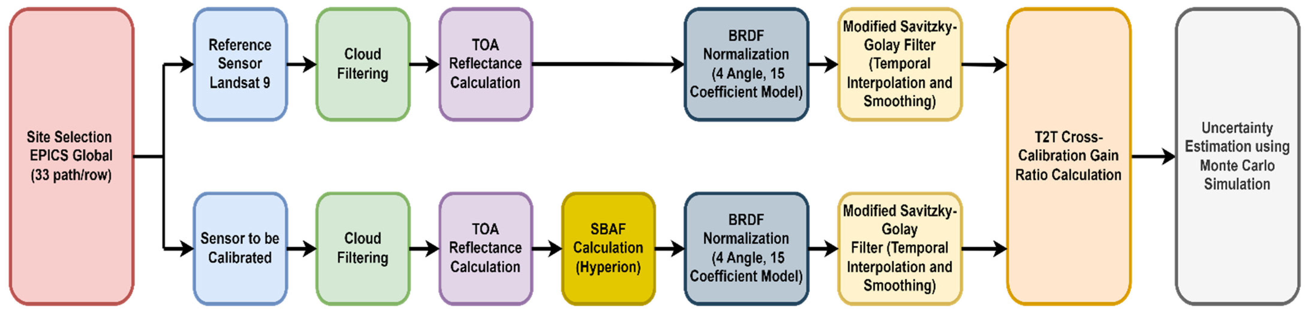
3. Methodology
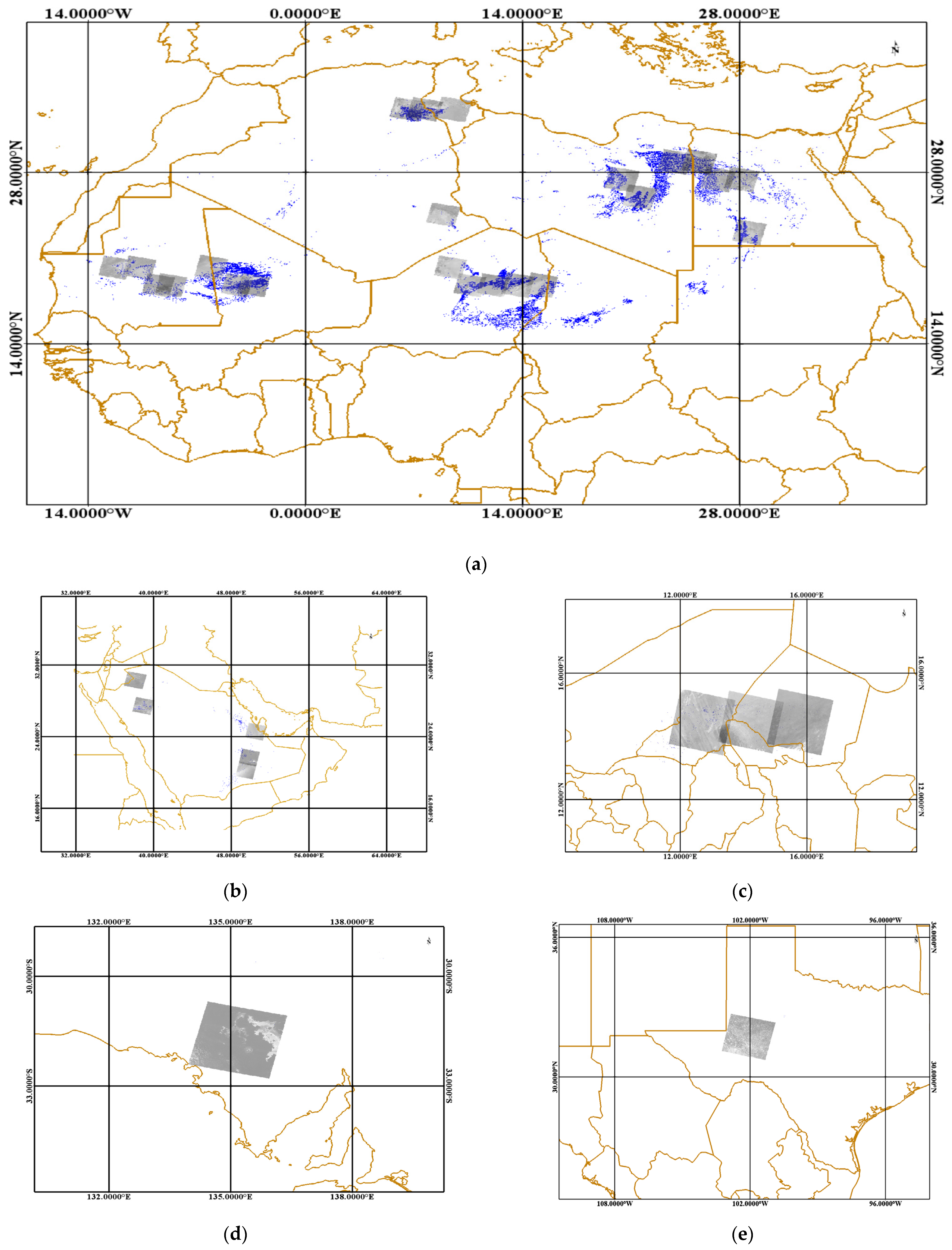
3.1. Site Selection
3.2. Cloud Screening from Scenes
3.3. TOA Reflectance Computation
3.3.1. Landsat Series TOA Reflectance
3.3.2. MODIS TOA Reflectance
3.3.3. Sentinel TOA Reflectance
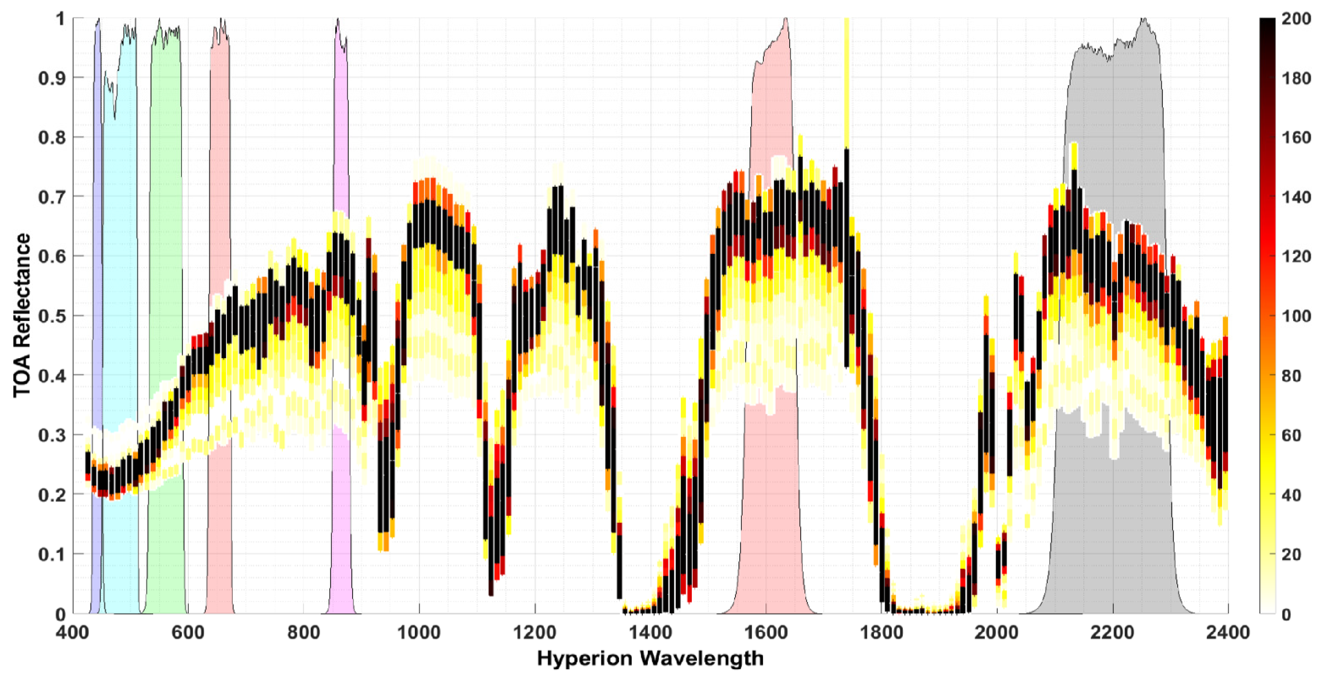
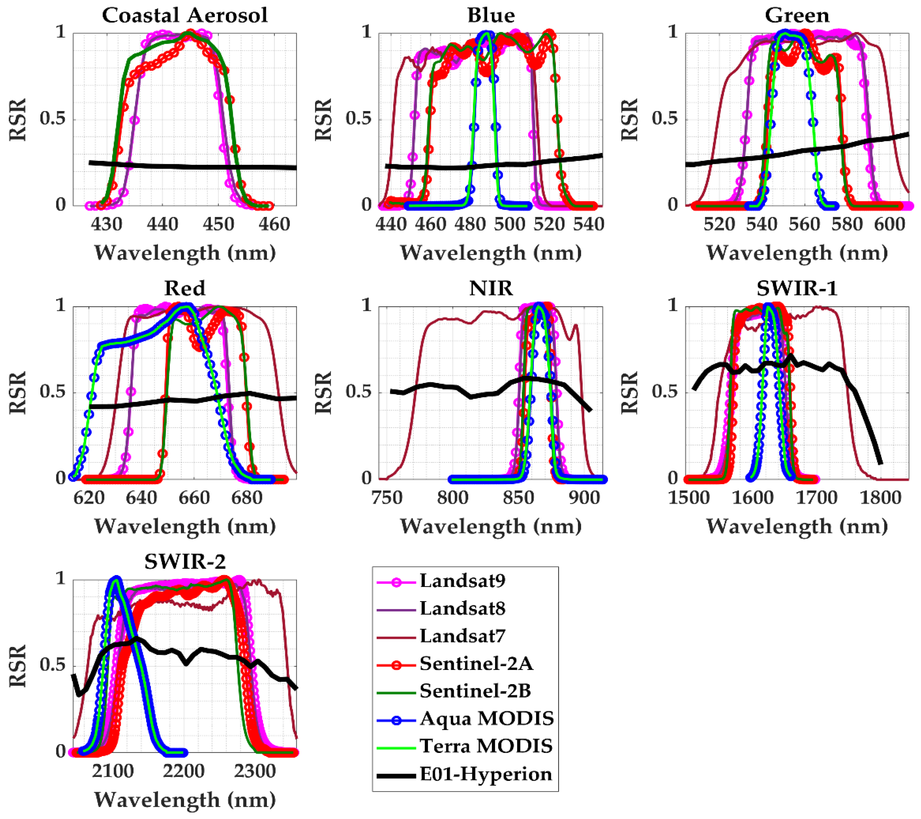
3.4. SBAF Calculation Using Hyperion
3.5. BRDF Normalization
3.6. Temporal Interpolation Using MSG Filter
3.7. Expanded T2T Cross-Calibration Gain
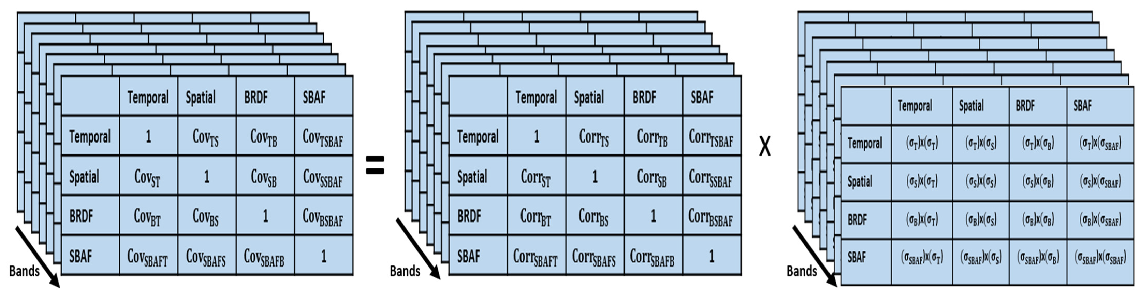
3.8. Uncertainty Estimation Using Monte Carlo Simulation
4. Validation of Expanded T2T Cross-Calibration Method
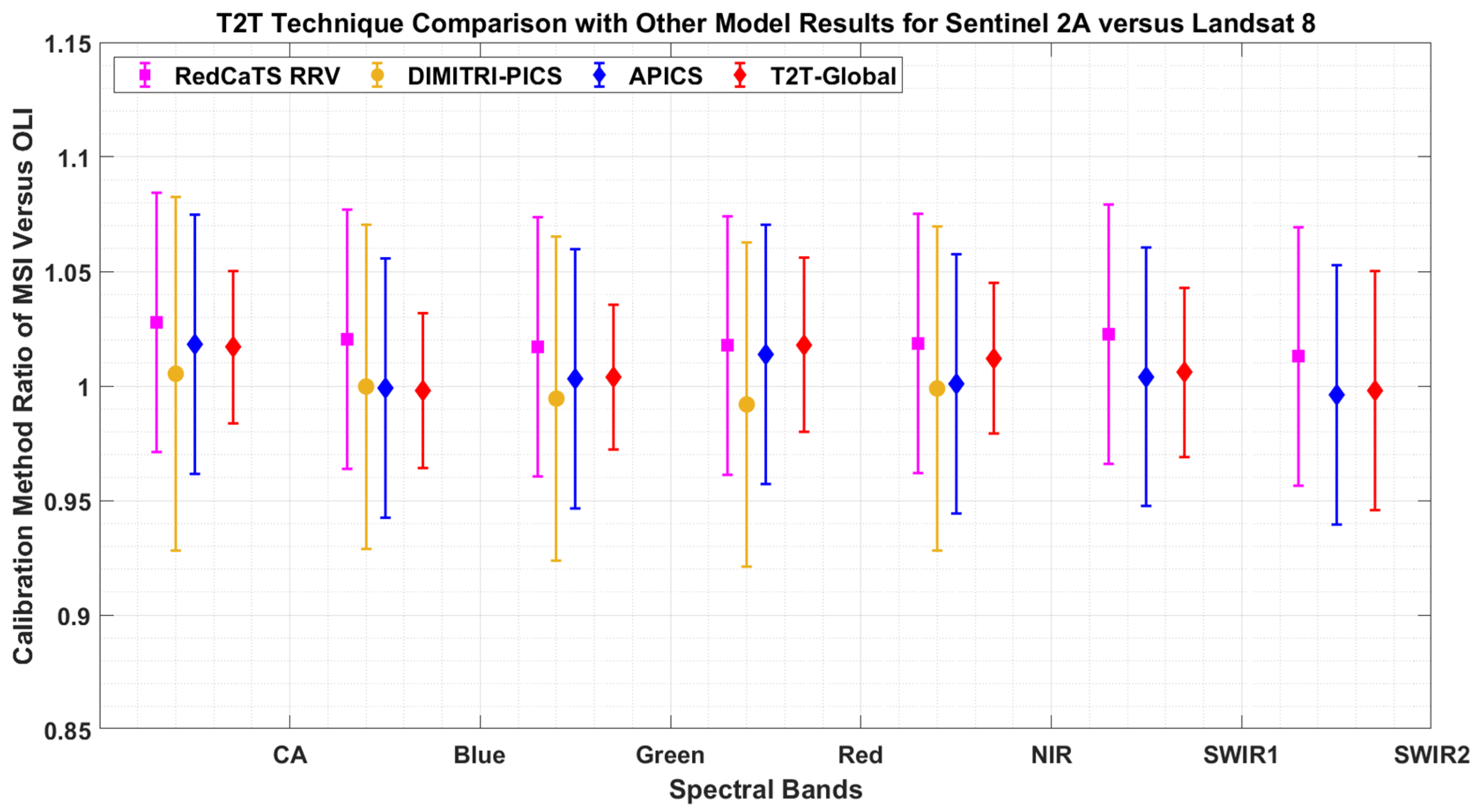
4.1. Expanded T2T Technique Validation Using Landsat 8 and Sentinel 2A
4.2. SDSU Inter-Comparison for Landsat 8 and Landsat 9
4.3. Expanded T2T Technique Validation Using ETM+ and Terra MODIS
5. Results and Discussion
5.1. Expanded T2T Cross-Calibration Application
5.1.1. Stepwise Results for Global Application
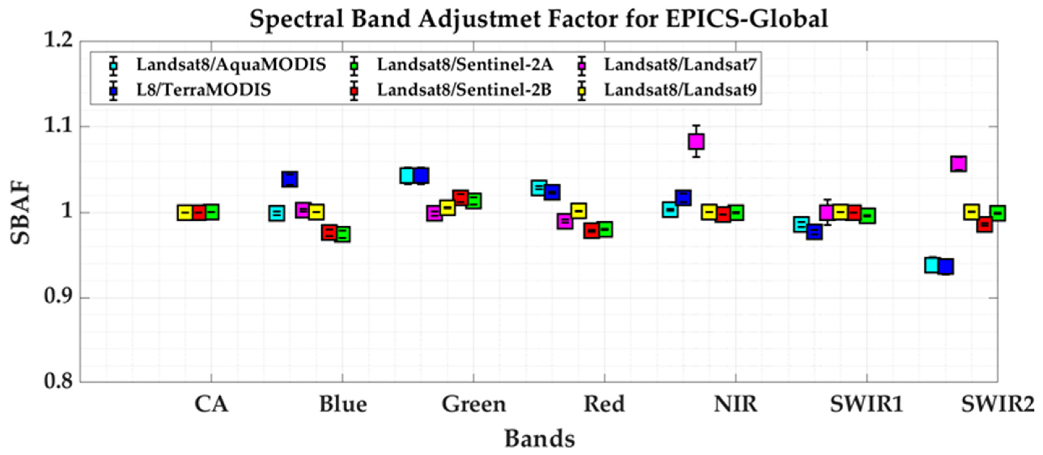
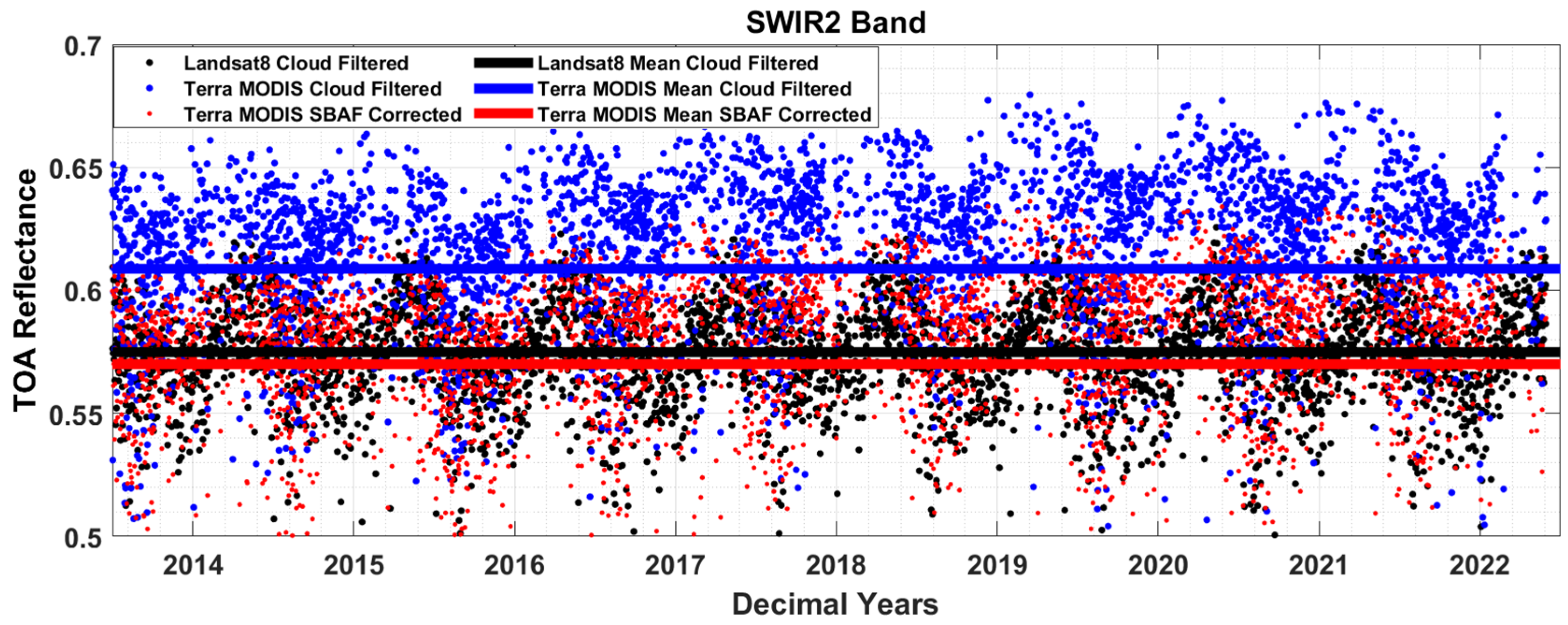
Global SBAF Estimation
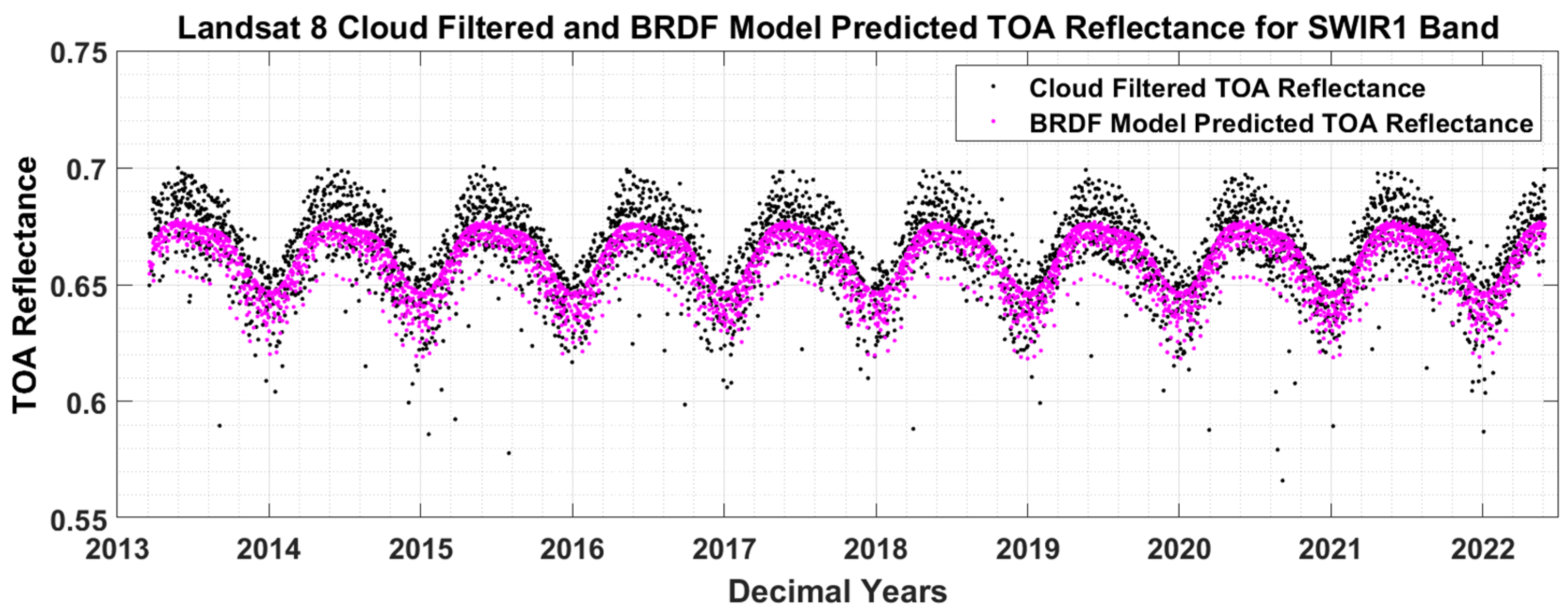
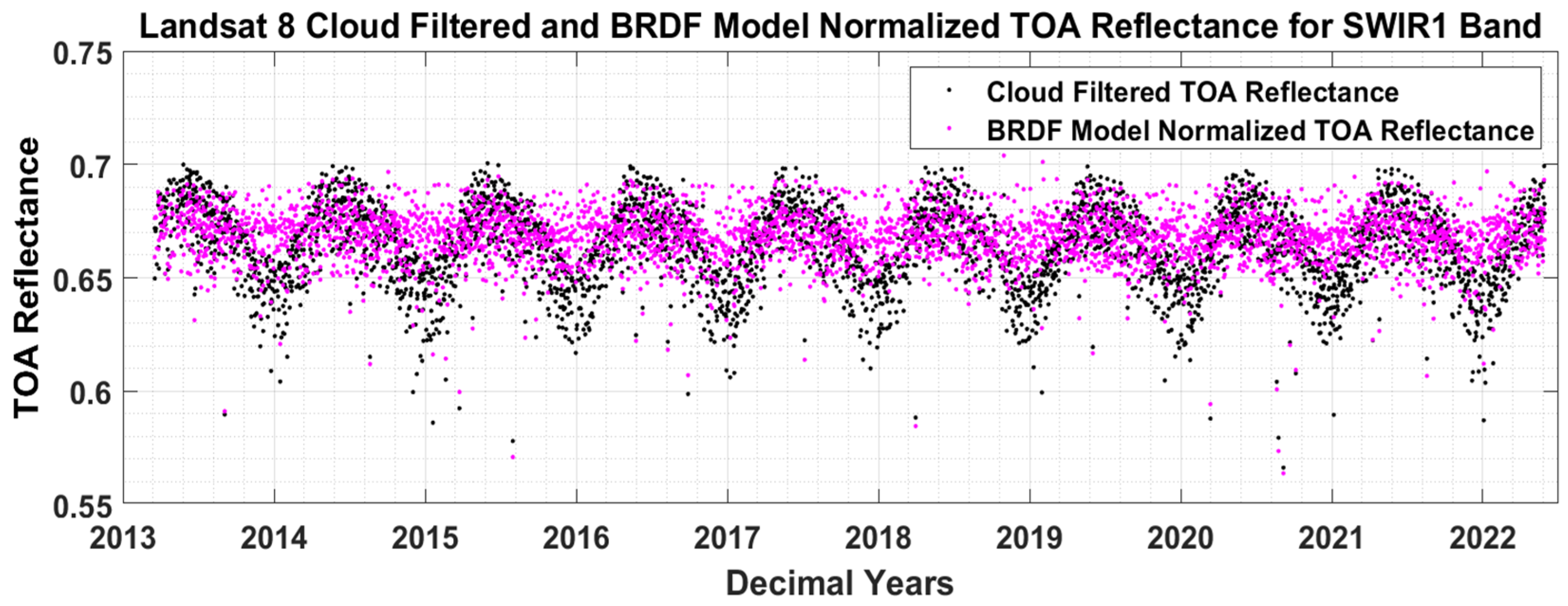
Cloud-Filtered and BRDF Normalized TOA Reflectance
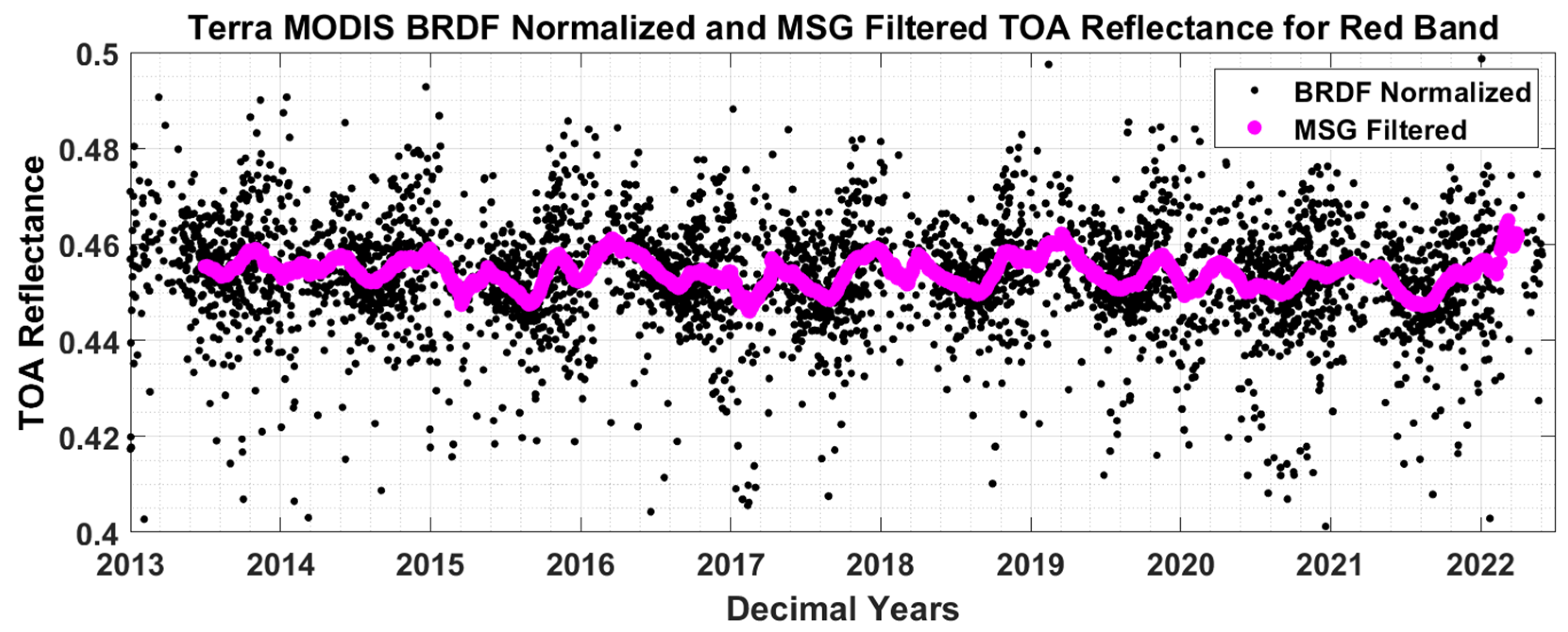
Trend Identification Using MSG Filter
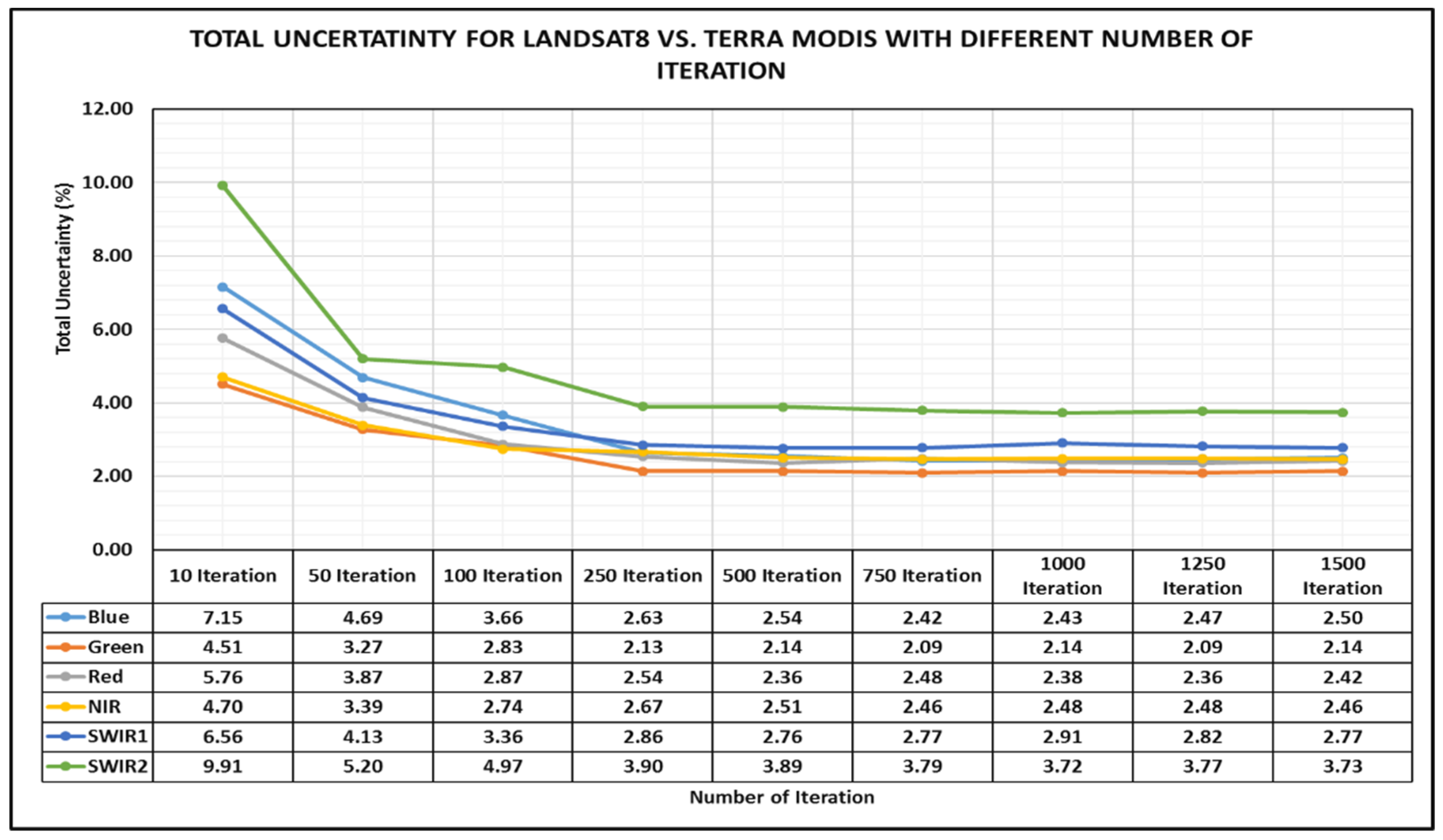
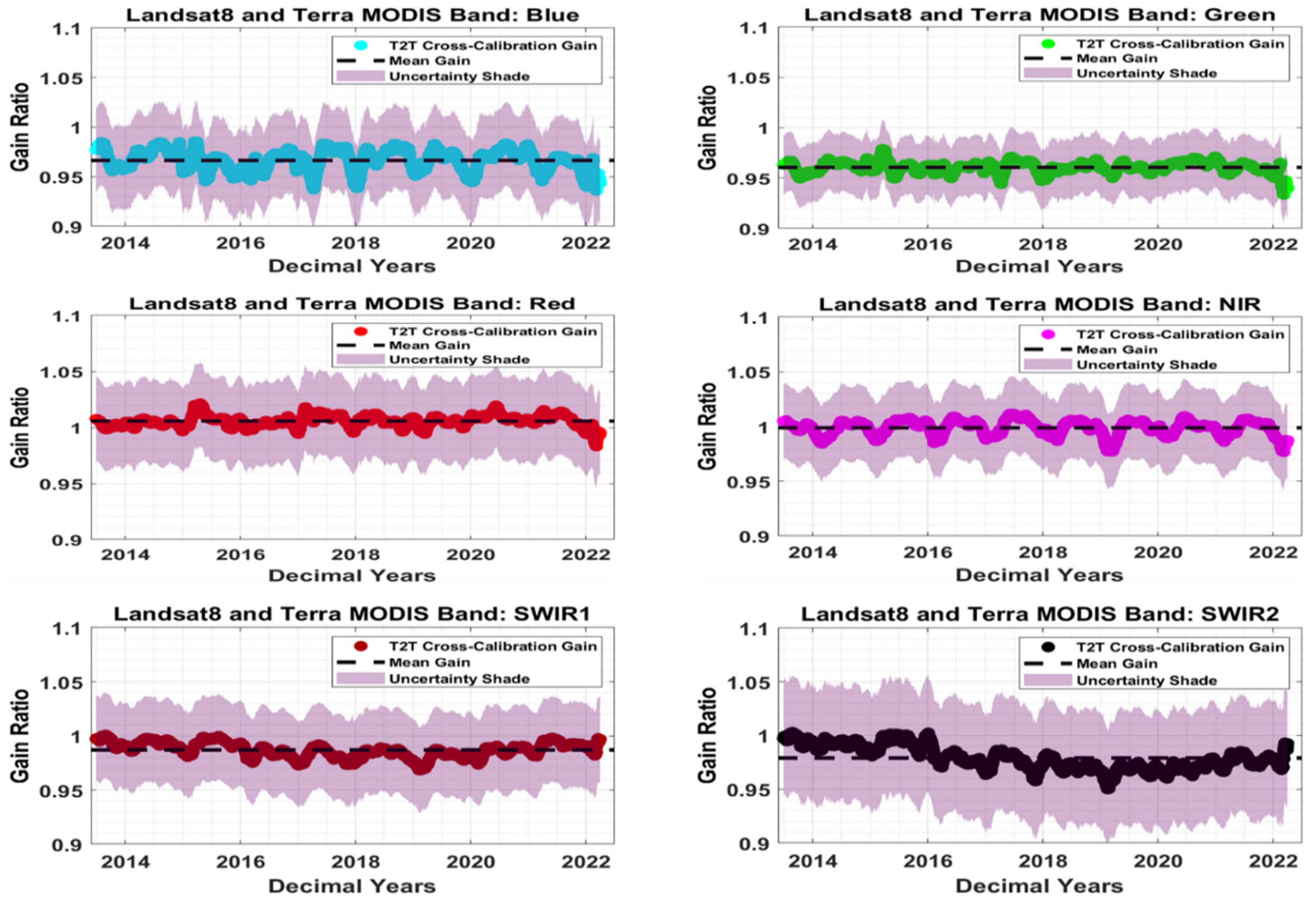
T2T Gain and Uncertainty Using Monte Carlo Simulation for Single Pair
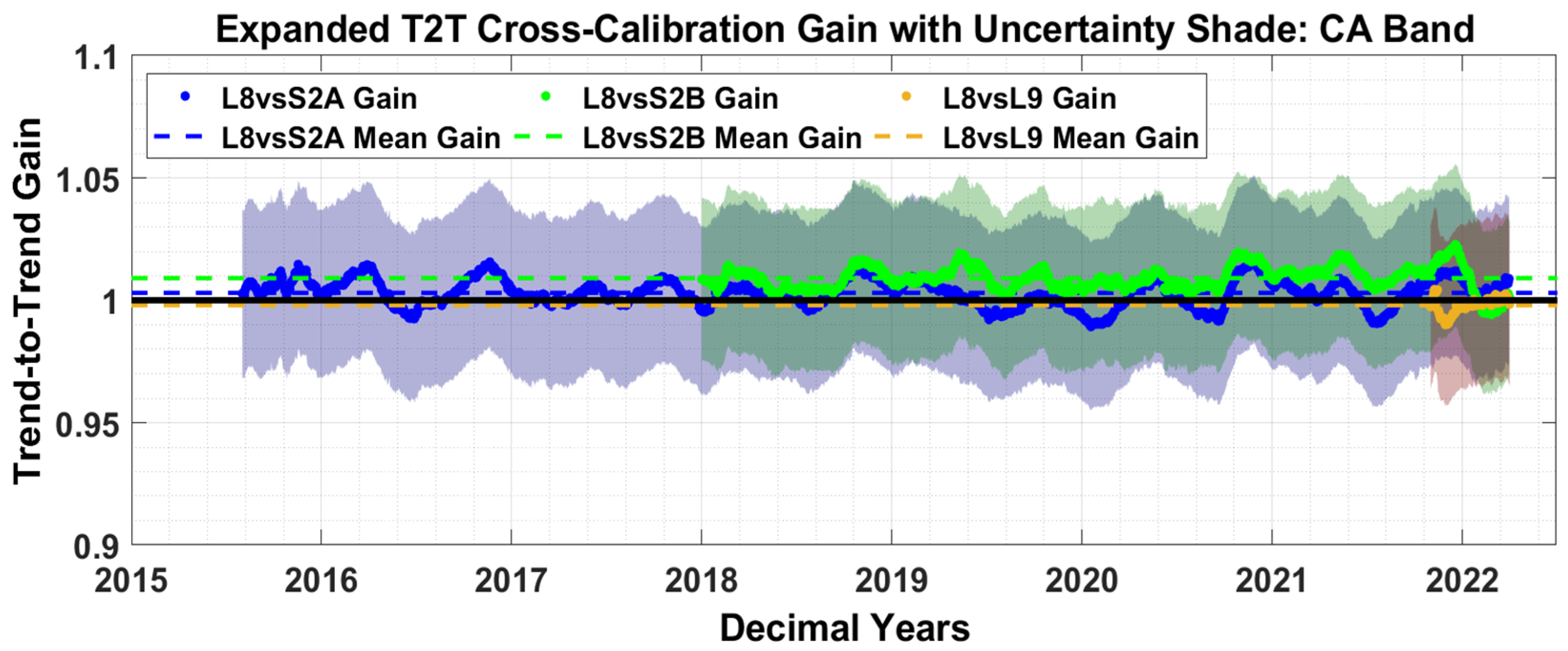
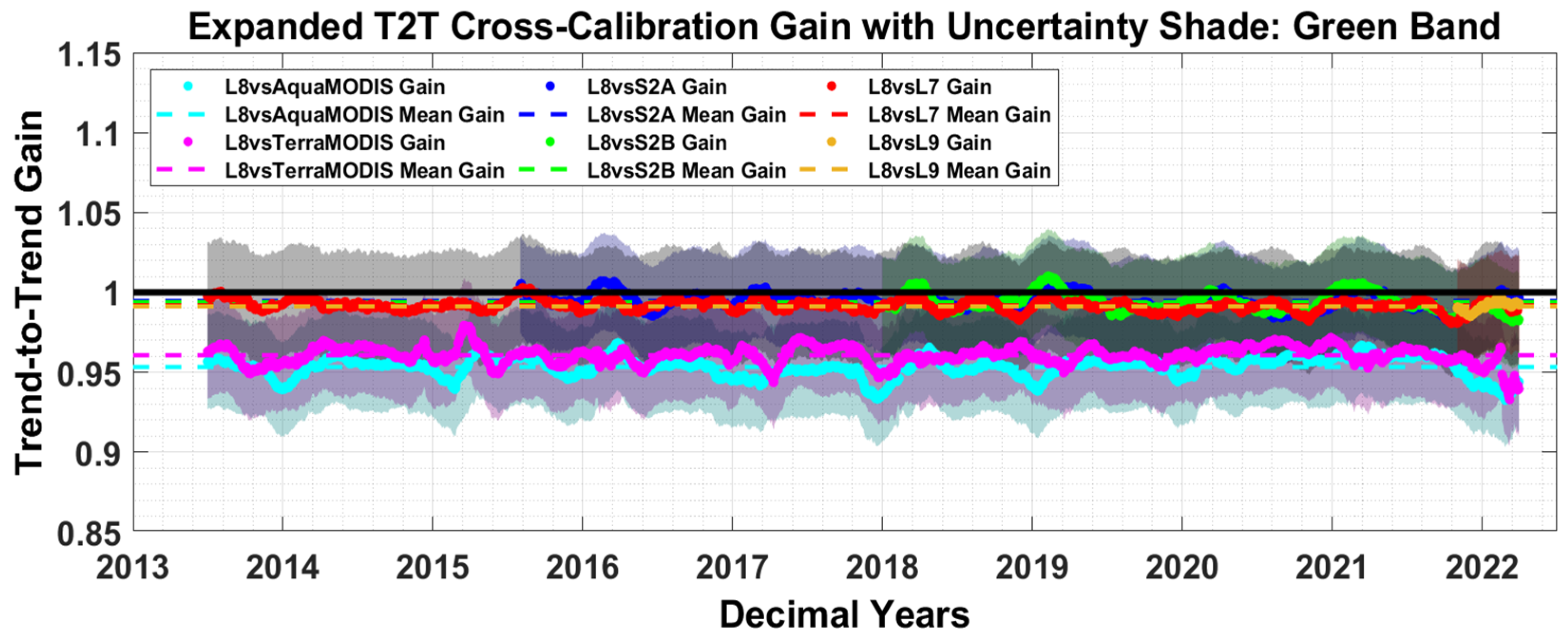
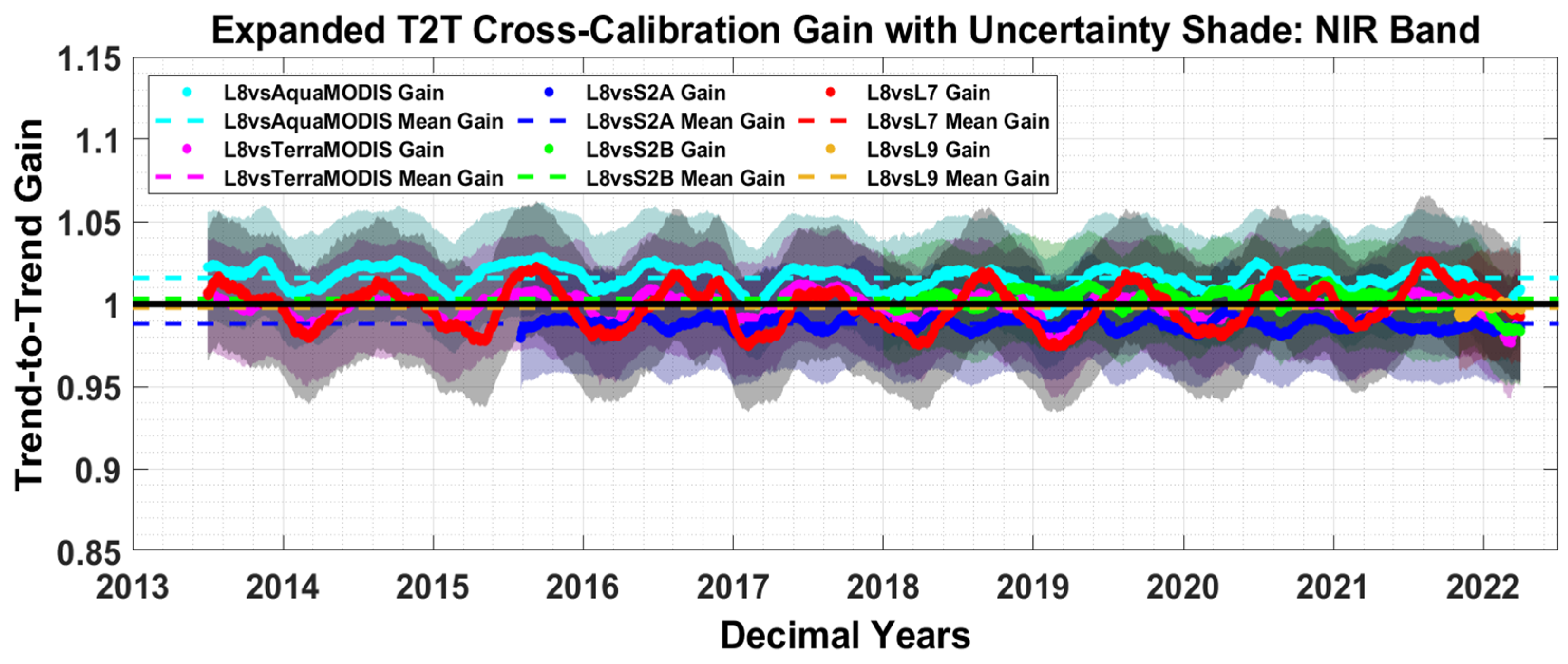
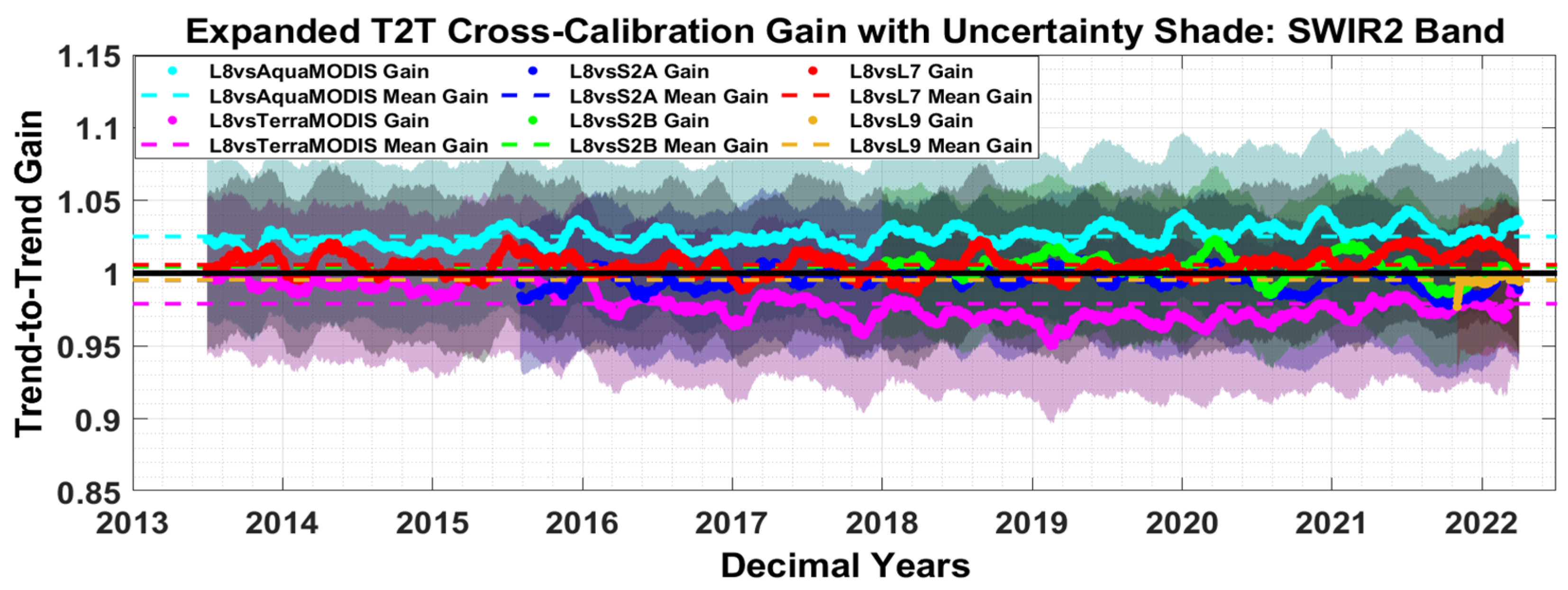
5.1.2. Combined T2T Cross-Calibration Result Using EPICS Global
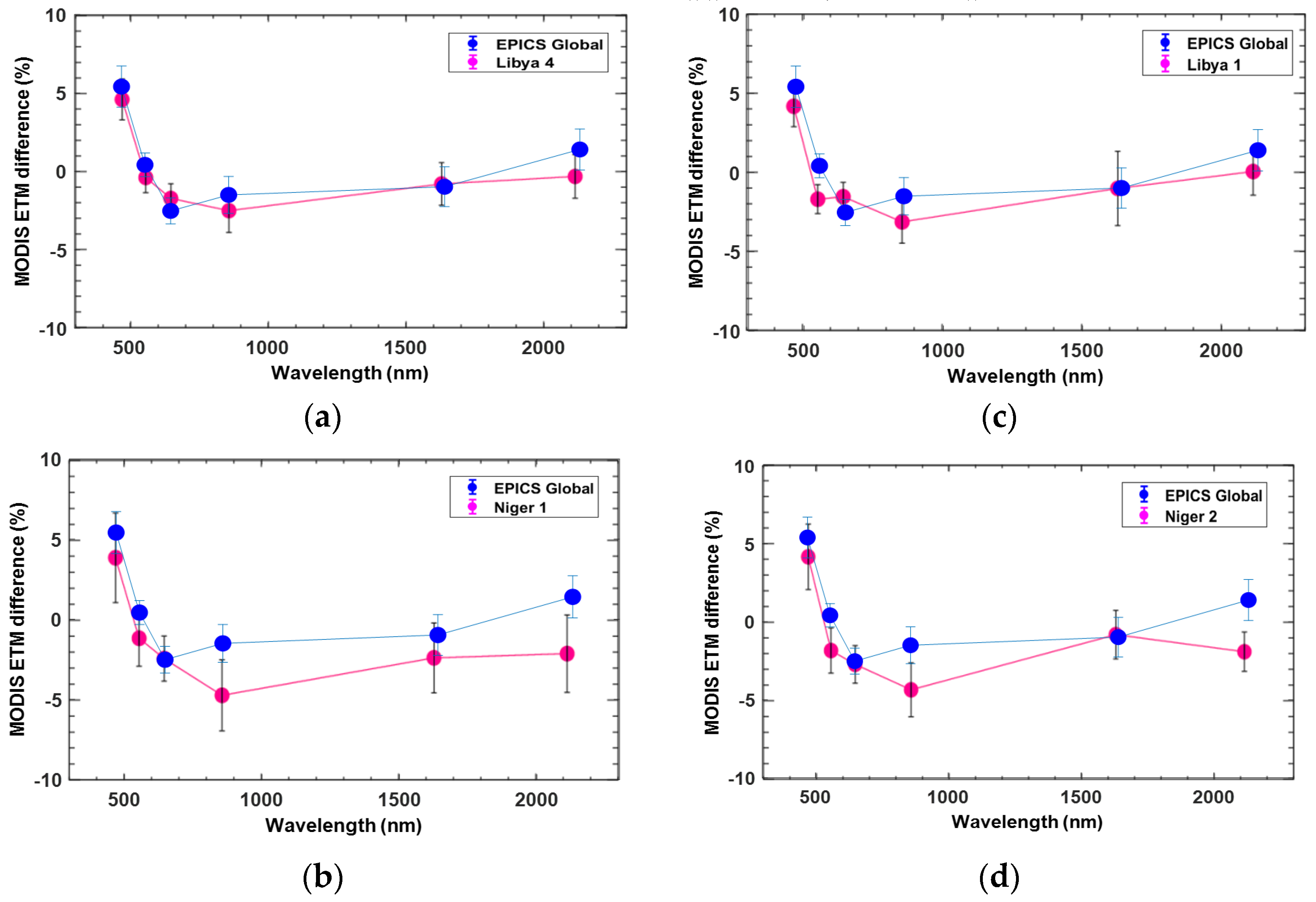
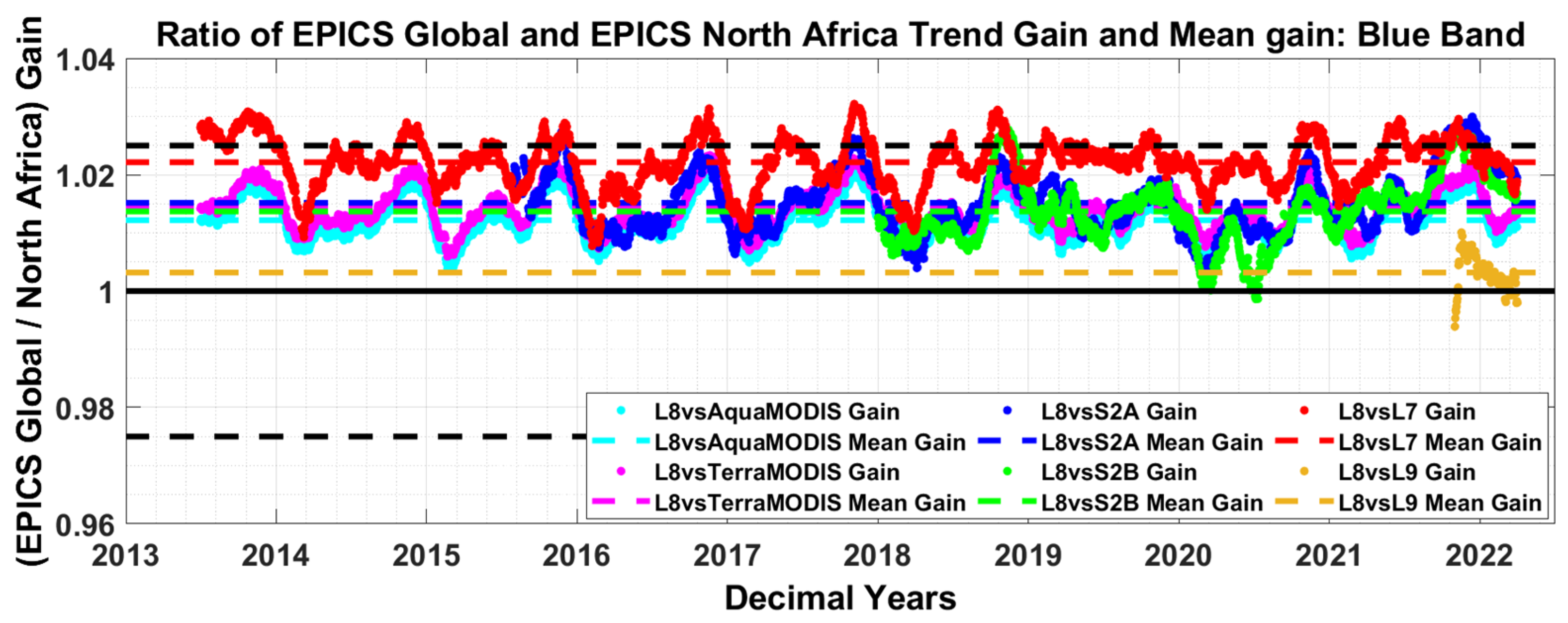
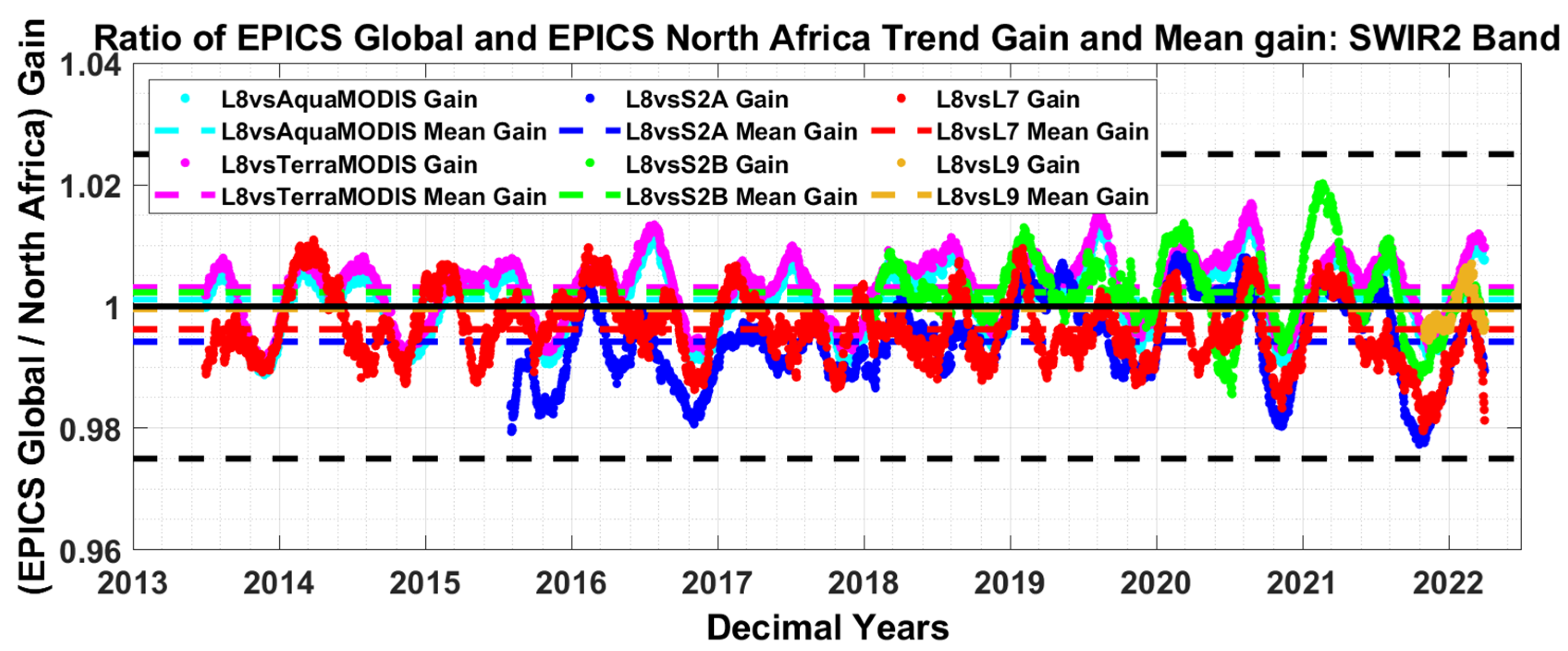
5.2. EPICS Global versus EPICS North Africa
6. Conclusions
Author Contributions
Funding
Data Availability Statement
Acknowledgments
Conflicts of Interest
References
- Wang, D.; Morton, D.; Masek, J.; Wu, A.; Nagol, J.; Xiong, X.; Levy, R.; Vermote, E.; Wolfe, R. Impact of sensor degradation on the MODIS NDVI time series. Remote Sens. Environ. 2012, 119, 55–61. [Google Scholar] [CrossRef] [Green Version]
- Barrientos, C.; Mattar, C.; Nakos, T.; Perez, W. Radiometric cross-calibration of the chilean satellite FASat-C using RapidEye and EO-1 hyperion data and a simultaneous nadir overpass approach. Remote Sens. 2016, 8, 612. [Google Scholar] [CrossRef] [Green Version]
- Markham, B.; Barsi, J.; Kvaran, G.; Ong, L.; Kaita, E.; Biggar, S.; Czapla-Myers, J.; Mishra, N.; Helder, D. Landsat-8 operational land imager radiometric calibration and stability. Remote Sens. 2014, 6, 12275–12308. [Google Scholar] [CrossRef] [Green Version]
- Dinguirard, M.; Slater, P.N. Calibration of space-multispectral imaging sensors: A review. Remote Sens. Environ. 1999, 68, 194–205. [Google Scholar] [CrossRef]
- Thorne, K.; Markharn, B.; Barker, P.S.; Biggar, S. Radiometric calibration of Landsat. Photogramm. Eng. Remote Sens. 1997, 63, 853–858. [Google Scholar]
- Chander, G.; Mishra, N.; Helder, D.L.; Aaron, D.B.; Angal, A.; Choi, T.; Xiong, X.; Doelling, D.R. Applications of spectral band adjustment factors (SBAF) for cross-calibration. IEEE Trans. Geosci. Remote Sens. 2012, 51, 1267–1281. [Google Scholar] [CrossRef]
- Helder, D.L.; Basnet, B.; Morstad, D.L. Optimized identification of worldwide radiometric pseudo-invariant calibration sites. Can. J. Remote Sens. 2010, 36, 527–539. [Google Scholar] [CrossRef]
- Teillet, P.; Chander, G. Terrestrial reference standard sites for postlaunch sensor calibration. Can. J. Remote Sens. 2010, 36, 437–450. [Google Scholar] [CrossRef]
- Bouvet, M. Radiometric comparison of multispectral imagers over a pseudo-invariant calibration site using a reference radiometric model. Remote Sens. Environ. 2014, 140, 141–154. [Google Scholar] [CrossRef]
- Vuppula, H. Normalization of Pseudo-Invariant Calibration Sites for Increasing the Temporal Resolution and Long-Term Trending; South Dakota State University: Brookings, SD, USA, 2017; Available online: https://openprairie.sdstate.edu/etd/2180/ (accessed on 15 April 2021).
- Shrestha, M.; Hasan, M.N.; Leigh, L.; Helder, D. Extended Pseudo Invariant Calibration Sites (EPICS) for the Cross-Calibration of Optical Satellite Sensors. Remote Sens. 2019, 11, 1676. [Google Scholar] [CrossRef] [Green Version]
- Shrestha, M.; Leigh, L.; Helder, D. Classification of north Africa for use as an extended pseudo invariant calibration sites (EPICS) for radiometric calibration and stability monitoring of optical satellite sensors. Remote Sens. 2019, 11, 875. [Google Scholar] [CrossRef]
- Hasan, M.N.; Shrestha, M.; Leigh, L.; Helder, D. Evaluation of an Extended PICS (EPICS) for calibration and stability monitoring of optical satellite sensors. Remote Sens. 2019, 11, 1755. [Google Scholar] [CrossRef] [Green Version]
- Khakurel, P.; Leigh, L.; Kaewmanee, M.; Pinto, C.T. Extended Pseudo Invariant Calibration Site-Based Trend-to-Trend Cross-Calibration of Optical Satellite Sensors. Remote Sens. 2021, 13, 1545. [Google Scholar] [CrossRef]
- Fajardo Rueda, J.; Leigh, L.; Teixeira Pinto, C.; Kaewmanee, M.; Helder, D. Classification and Evaluation of Extended PICS (EPICS) on a Global Scale for Calibration and Stability Monitoring of Optical Satellite Sensors. Remote Sens. 2021, 13, 3350. [Google Scholar] [CrossRef]
- Gross, G.; Helder, D.; Begeman, C.; Leigh, L.; Kaewmanee, M.; Shah, R. Initial Cross-Calibration of Landsat 8 and Landsat 9 Using the Simultaneous Underfly Event. Remote Sens. 2022, 14, 2418. [Google Scholar] [CrossRef]
- Goward, S.N.; Masek, J.G.; Williams, D.L.; Irons, J.R.; Thompson, R. The Landsat 7 mission: Terrestrial research and applications for the 21st century. Remote Sens. Environ. 2001, 78, 3–12. [Google Scholar] [CrossRef]
- Andrefouet, S.; Bindschadler, R.; Brown de Colstoun, E.; Choate, M.; Chomentowski, W.; Christopherson, J.; Doorn, B.; Hall, D.; Holifield, C.; Howard, S. Preliminary Assessment of the Value of Landsat-7 ETM+ Data Following Scan Line Corrector Malfunction; U.S. Geological Survey's EROS Data Center: Sioux Falls, SD, USA, 2003. Available online: https://www.usgs.gov/media/files/preliminaryassessment-value-landsat-7-etm-slc-data (accessed on 15 April 2021).
- Irons, J.R.; Dwyer, J.L.; Barsi, J.A. The next Landsat satellite: The Landsat data continuity mission. Remote Sens. Environ. 2012, 122, 11–21. [Google Scholar] [CrossRef] [Green Version]
- Xiong, X.; Sun, J.; Xie, X.; Barnes, W.L.; Salomonson, V.V. On-orbit calibration and performance of Aqua MODIS reflective solar bands. IEEE Trans. Geosci. Remote Sens. 2009, 48, 535–546. [Google Scholar] [CrossRef]
- Xiong, X.; Chiang, K.-F.; Wu, A.; Barnes, W.L.; Guenther, B.; Salomonson, V.V. Multiyear on-orbit calibration and performance of Terra MODIS thermal emissive bands. IEEE Trans. Geosci. Remote Sens. 2008, 46, 1790–1803. [Google Scholar] [CrossRef] [Green Version]
- Drusch, M.; Del Bello, U.; Carlier, S.; Colin, O.; Fernandez, V.; Gascon, F.; Hoersch, B.; Isola, C.; Laberinti, P.; Martimort, P. Sentinel-2: ESA’s optical high-resolution mission for GMES operational services. Remote Sens. Environ. 2012, 120, 25–36. [Google Scholar] [CrossRef]
- Barsi, J.A.; Alhammoud, B.; Czapla-Myers, J.; Gascon, F.; Haque, M.O.; Kaewmanee, M.; Leigh, L.; Markham, B.L. Sentinel-2A MSI and Landsat-8 OLI radiometric cross comparison over desert sites. Eur. J. Remote Sens. 2018, 51, 822–837. [Google Scholar] [CrossRef]
- Guo, Y.; Li, L.; Jin, L.; Wang, K. Study on cloud processing methods with MODIS data. In Proceedings of the 2013 5th IEEE International Symposium on Microwave, Antenna, Propagation and EMC Technologies for Wireless Communications, Chengdu, China, 29–31 October 2013; pp. 694–696. [Google Scholar] [CrossRef]
- Shrestha, M.; Hasan, N.; Leigh, L.; Helder, D. Derivation of Hyperspectral Profile of Extended Pseudo Invariant Calibration Sites (EPICS) for Use in Sensor Calibration. Remote Sens. 2019, 11, 2279. [Google Scholar] [CrossRef] [Green Version]
- Jing, X.; Leigh, L.; Helder, D.; Pinto, C.T.; Aaron, D. Lifetime absolute calibration of the EO-1 Hyperion sensor and its validation. IEEE Trans. Geosci. Remote Sens. 2019, 57, 9466–9475. [Google Scholar] [CrossRef]
- Collings, S.; Caccetta, P.; Campbell, N.; Wu, X. Techniques for BRDF correction of hyperspectral mosaics. IEEE Trans. Geosci. Remote Sens. 2010, 48, 3733–3746. [Google Scholar] [CrossRef]
- Helder, D.; Thome, K.J.; Mishra, N.; Chander, G.; Xiong, X.; Angal, A.; Choi, T. Absolute radiometric calibration of Landsat using a pseudo invariant calibration site. IEEE Trans. Geosci. Remote Sens. 2013, 51, 1360–1369. [Google Scholar] [CrossRef]
- Farhad, M.; Kaewmanee, M.; Leigh, L.; Helder, D. Radiometric cross calibration and validation using 4 angle BRDF model between landsat 8 and sentinel 2A. Remote Sens. 2020, 12, 806. [Google Scholar] [CrossRef]
- Kaewmanee, M. Pseudo Invariant Calibration Sites: PICS Evolution. In Proceedings of the CALCON 2018, Logan, UT, USA, 18–20 June 2018. [Google Scholar]
- Savitzky, A.; Golay, M.J. Smoothing and differentiation of data by simplified least squares procedures. Anal. Chem. 1964, 36, 1627–1639. [Google Scholar] [CrossRef]
- TaubenbockTaubenbock, H.; Habermeyer, M.; Roth, A.; Dech, S. Automated allocation of highly structured urban areas in homogeneous zones from remote sensing data by Savitzky–Golay filtering and curve sketching. IEEE Geosci. Remote Sens. Lett. 2006, 3, 532–536. [Google Scholar] [CrossRef]
- Pinto, C.T.; Ponzoni, F.J.; Castro, R.M.; Leigh, L.; Kaewmanee, M.; Aaron, D.; Helder, D. Evaluation of the uncertainty in the spectral band adjustment factor (SBAF) for cross-calibration using Monte Carlo simulation. Remote Sens. Lett. 2016, 7, 837–846. [Google Scholar] [CrossRef]
- Czapla-Myers, J.; McCorkel, J.; Anderson, N.; Thome, K.; Biggar, S.; Helder, D.; Aaron, D.; Leigh, L.; Mishra, N. The ground-based absolute radiometric calibration of Landsat 8 OLI. Remote Sens. 2015, 7, 600–626. [Google Scholar] [CrossRef]
- Francesconi, B.; Neveu-VanMalle, M.; Espesset, A.; Alhammoud, B.; Bouzinac, C.; Clerc, S.; Gascon, F. Image quality validation of sentinel 2 level-1 products: Performance status at the beginning of the constellation routine phase. In Proceedings of the Sensors, Systems, and Next-Generation Satellites XXI, Warsaw, Poland, 11–14 September 2017; pp. 44–61. [Google Scholar] [CrossRef]
- Choi, J.; Xiong, X.; Mishra, N.; Helder, D.; Angal, A. Absolute Calibration of Optical Satellite Sensors Using Libya 4 Pseudo Invariant Calibration Site. Remote Sens. 2014, 6, 1327–1346. [Google Scholar] [CrossRef] [Green Version]
- Angal, A.; Xiong, X.; Helder, D.; Kaewmanee, M.; Leigh, L. Assessing the calibration differences in the reflective solar bands of Terra MODIS and Landsat-7 enhanced thematic mapper plus. J. Appl. Remote Sens. 2018, 12, 044002. [Google Scholar] [CrossRef]
- Xiong, X.; Angal, A.; Li, Y.; Twedt, K. Improvements of on-orbit characterization of Terra MODIS short-wave infrared spectral bands out-of-band responses. J. Appl. Remote Sens. 2020, 14, 047503. [Google Scholar] [CrossRef]


| Characteristics | Sensors | |||
|---|---|---|---|---|
| Landsat 8/9 | Landsat 7 | Sentinel 2A/2B | MODIS Terra/Aqua | |
| Launch Date | 11 February 2012/ 27 September 2021 | 15 April 1999 | 23 June 2015/ 7 March 2018 | 18 December 1999/ 4 May 2002 |
| Number of Bands | 11 (1 pan, 8 multispectral, 2 thermal) | 8 (1 pan, 6 multispectral, 1 thermal) | 13 (All multispectral) | 36 (Spectral Bands) |
| Spatial Resolution | 15, 30, 100 (m) (pan, multispectral, thermal) | 15, 30, 60 (m) (pan, multispectral, thermal) | 10, 20, 60 (m) (All multispectral) | 250, 500, 1000 (m) (Bands 1–2, 3–7, 8–36) |
| Equatorial crossing time | 10:00–10:15 | 10:00–10:15 | 10:30 | 10:30 |
| Swath width | 183 (km) | 183 (km) | 290 (km) | 2330 (km) |
| Revisit frequency | 16 (days) | 16 (days) | 10 (days) | 1–2 (days) |
| Orbit altitude | 705 (km) | 705 (km) | 785 (km) | 705 (km) |
| Xcal Ratio | CA | Blue | Green | Red | NIR | SWIR1 | SWIR2 |
|---|---|---|---|---|---|---|---|
| Underfly | 1.0010 | 1.0020 | 0.9960 | 1.0000 | 1.0010 | 1.0030 | 1.0040 |
| ExPAC-NA | 0.9927 | 0.9948 | 0.9898 | 0.9945 | 0.9963 | 0.9963 | 0.9992 |
| XCal-NA | 0.9935 | 0.9943 | 0.9916 | 0.997 | 0.9979 | 0.9969 | 1.0008 |
| XCal-Global | 0.9938 | 0.9942 | 0.9935 | 1.0028 | 1.0006 | 0.9979 | 0.9983 |
| T2T-NA | 0.9955 | 0.9939 | 0.9895 | 0.9941 | 0.9958 | 0.9987 | 0.9937 |
| T2T-Global | 0.9970 | 0.9968 | 0.9915 | 0.9974 | 0.9967 | 0.9980 | 0.9951 |
| Adjusted Gain | 0.9967 | 0.9966 | 0.9921 | 0.9975 | 0.9979 | 0.9977 | 0.9981 |
| Uncertainty Source (%) | Bands | |||||
|---|---|---|---|---|---|---|
| Blue | Green | Red | NIR | SWIR1 | SWIR2 | |
| Landsat 8 Calibration | 2 | 2 | 2 | 2 | 2 | 2 |
| Temporal | 2.00 | 1.53 | 1.64 | 1.23 | 1.31 | 2.86 |
| Spatial | 1.56 | 1.64 | 1.84 | 2.09 | 2.55 | 2.67 |
| SBAF | 1.87 | 1.41 | 1.61 | 1.25 | 1.36 | 2.66 |
| BRDF | 0.29 | 0.27 | 0.28 | 0.29 | 0.27 | 0.26 |
| Total | 2.52 | 2.09 | 2.45 | 2.38 | 2.89 | 3.77 |
| Gain and Uncertainty | Sensors Pairs | Bands | ||||||
|---|---|---|---|---|---|---|---|---|
| CA | Blue | Green | Red | NIR | SWIR1 | SWIR2 | ||
| Gain | L8 vs. Aqua MODIS | ---- | 0.9496 | 0.9533 | 0.9872 | 1.0158 | 1.0009 | 1.0253 |
| Uncertainty (%) | ---- | 2.49 | 2.14 | 2.48 | 2.42 | 2.87 | 3.84 | |
| Gain | L8 vs. Terra MODIS | ---- | 0.9664 | 0.9606 | 1.0058 | 0.9988 | 0.9870 | 0.9791 |
| Uncertainty (%) | ---- | 2.52 | 2.09 | 0.45 | 2.38 | 2.89 | 3.77 | |
| Gain | L8 vs. Sentinel2A | 1.0030 | 1.0168 | 0.9947 | 0.9815 | 0.9881 | 0.9939 | 0.9952 |
| Uncertainty (%) | 3.32 | 3.37 | 3.16 | 3.80 | 3.29 | 3.73 | 5.23 | |
| Gain | L8 vs. Sentinel2B | 1.0091 | 1.0136 | 0.9939 | 0.9733 | 1.0031 | 0.9940 | 1.0044 |
| Uncertainty (%) | 3.41 | 3.39 | 3.08 | 3.74 | 3.30 | 3.68 | 4.99 | |
| Gain | L8 vs. L9 | 0.9980 | 0.9978 | 0.9912 | 0.9971 | 0.9977 | 0.9981 | 0.9954 |
| Uncertainty (%) | 3.45 | 3.44 | 3.01 | 3.45 | 3.23 | 3.68 | 5.13 | |
| Gain | L8 vs. L7 | ---- | 1.0249 | 0.9919 | 0.9760 | 0.9987 | 1.0234 | 1.0058 |
| Uncertainty (%) | ---- | 3.39 | 3.28 | 2.93 | 4.11 | 3.69 | 5.10 | |
| The Ratio of EPICS Global and North Africa Mean Gain | Bands | ||||||
|---|---|---|---|---|---|---|---|
| CA | Blue | Green | Red | NIR | SWIR1 | SWIR2 | |
| L8 vs. Aqua MODIS | ---- | 1.0122 | 0.9936 | 0.9810 | 0.9932 | 1.0035 | 1.0011 |
| L8 vs. Terra MODIS | ---- | 1.0143 | 0.9957 | 0.9829 | 0.9952 | 1.0052 | 1.0032 |
| L8 vs. Sentinel2A | 1.0158 | 1.0152 | 0.9920 | 0.9802 | 0.9908 | 0.9989 | 0.9942 |
| L8 vs. Sentinel2B | 1.0150 | 1.0137 | 0.9937 | 0.9834 | 0.9946 | 1.0009 | 1.0023 |
| L8 vs. L9 | 1.0034 | 1.0032 | 1.0012 | 1.0041 | 1.0017 | 0.9989 | 0.9995 |
| L8 vs. L7 | ---- | 1.0221 | 0.9922 | 0.9985 | 1.0025 | 0.9945 | 0.9962 |
| Sensors Pairs | EPICS Global Total Uncertainty | EPICS North Africa Total Uncertainty | ||||||||||||
|---|---|---|---|---|---|---|---|---|---|---|---|---|---|---|
| CA | Blue | Green | Red | NIR | SWIR1 | SWIR2 | CA | Blue | Green | Red | NIR | SWIR1 | SWIR2 | |
| L8 vs. Aqua MODIS | ---- | 2.49 | 2.14 | 2.48 | 2.42 | 2.87 | 3.84 | ---- | 2.58 | 2.33 | 3.08 | 2.54 | 3.19 | 3.89 |
| L8 vs. Terra MODIS | ---- | 2.52 | 2.09 | 2.45 | 2.38 | 2.89 | 3.77 | ---- | 2.67 | 2.32 | 2.96 | 2.56 | 3.28 | 3.80 |
| L8 vs. Sentinel2A | 3.32 | 3.37 | 3.16 | 3.80 | 3.29 | 3.73 | 5.23 | 3.03 | 3.17 | 2.55 | 3.04 | 2.55 | 3.43 | 4.62 |
| L8 vs. Sentinel2B | 3.41 | 3.39 | 3.08 | 3.74 | 3.30 | 3.68 | 4.99 | 3.10 | 3.09 | 2.58 | 3.03 | 2.63 | 3.34 | 4.74 |
| L8 vs. L9 | 3.45 | 3.44 | 3.01 | 3.45 | 3.23 | 3.68 | 5.13 | 3.14 | 3.32 | 2.52 | 3.04 | 2.69 | 3.50 | 4.59 |
| L8 vs. L7 | ---- | 3.39 | 3.28 | 2.93 | 4.11 | 3.69 | 5.10 | ---- | 3.05 | 3.06 | 2.51 | 3.44 | 2.91 | 4.63 |
Publisher’s Note: MDPI stays neutral with regard to jurisdictional claims in published maps and institutional affiliations. |
© 2022 by the authors. Licensee MDPI, Basel, Switzerland. This article is an open access article distributed under the terms and conditions of the Creative Commons Attribution (CC BY) license (https://creativecommons.org/licenses/by/4.0/).
Share and Cite
Shah, R.; Leigh, L.; Kaewmanee, M.; Pinto, C.T. Validation of Expanded Trend-to-Trend Cross-Calibration Technique and Its Application to Global Scale. Remote Sens. 2022, 14, 6216. https://doi.org/10.3390/rs14246216
Shah R, Leigh L, Kaewmanee M, Pinto CT. Validation of Expanded Trend-to-Trend Cross-Calibration Technique and Its Application to Global Scale. Remote Sensing. 2022; 14(24):6216. https://doi.org/10.3390/rs14246216
Chicago/Turabian StyleShah, Ramita, Larry Leigh, Morakot Kaewmanee, and Cibele Teixeira Pinto. 2022. "Validation of Expanded Trend-to-Trend Cross-Calibration Technique and Its Application to Global Scale" Remote Sensing 14, no. 24: 6216. https://doi.org/10.3390/rs14246216