
Research on Self-Noise Suppression of Marine Acoustic Sensor Arrays

 , , , , and
Abstract
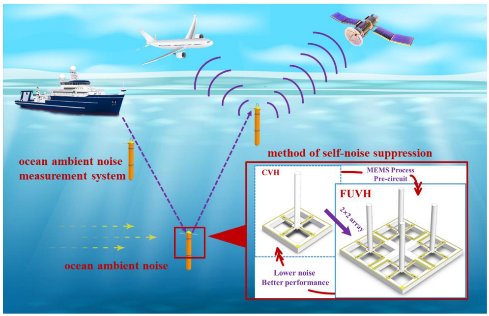
:1. Introduction
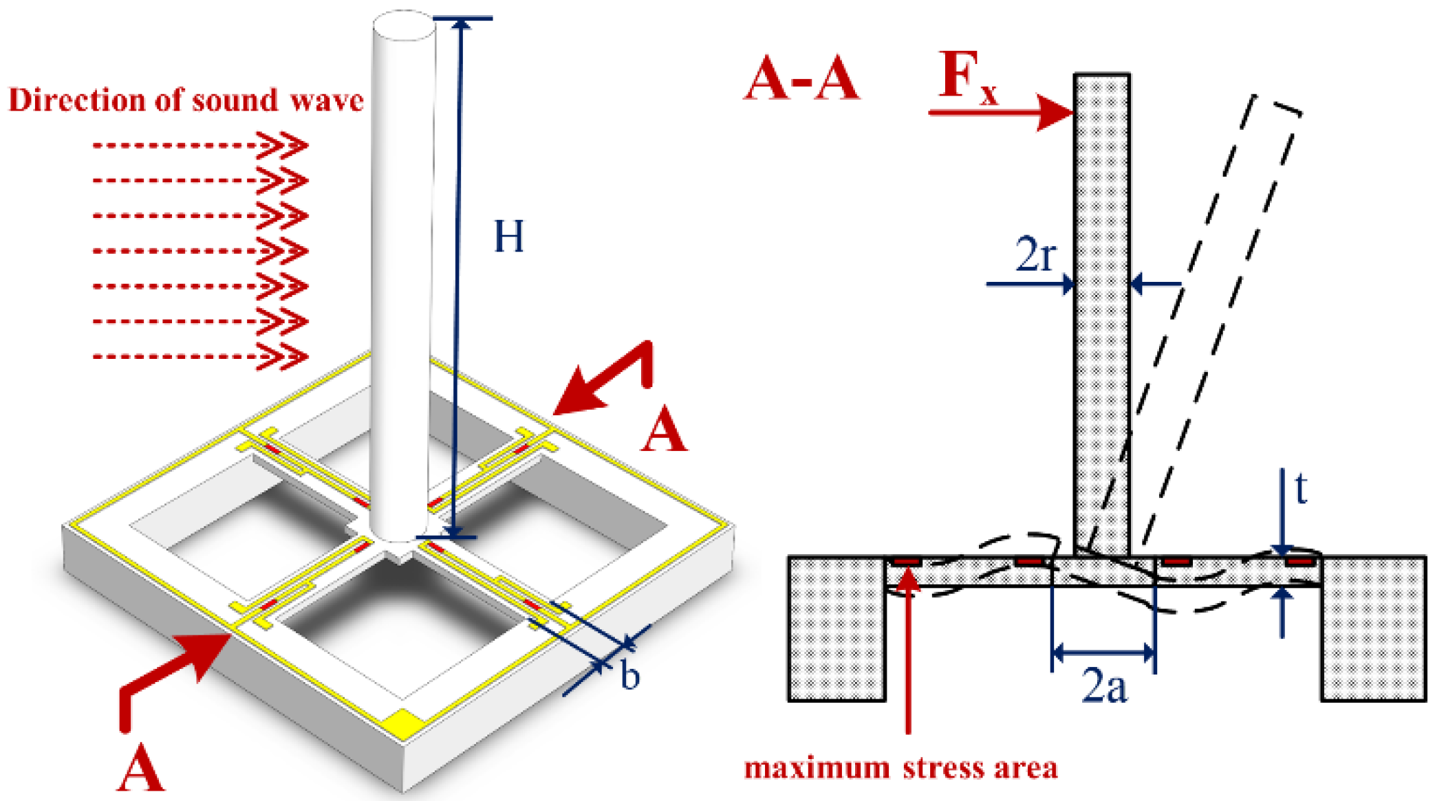
2. Sensitivity Principle
3. Noise Analysis
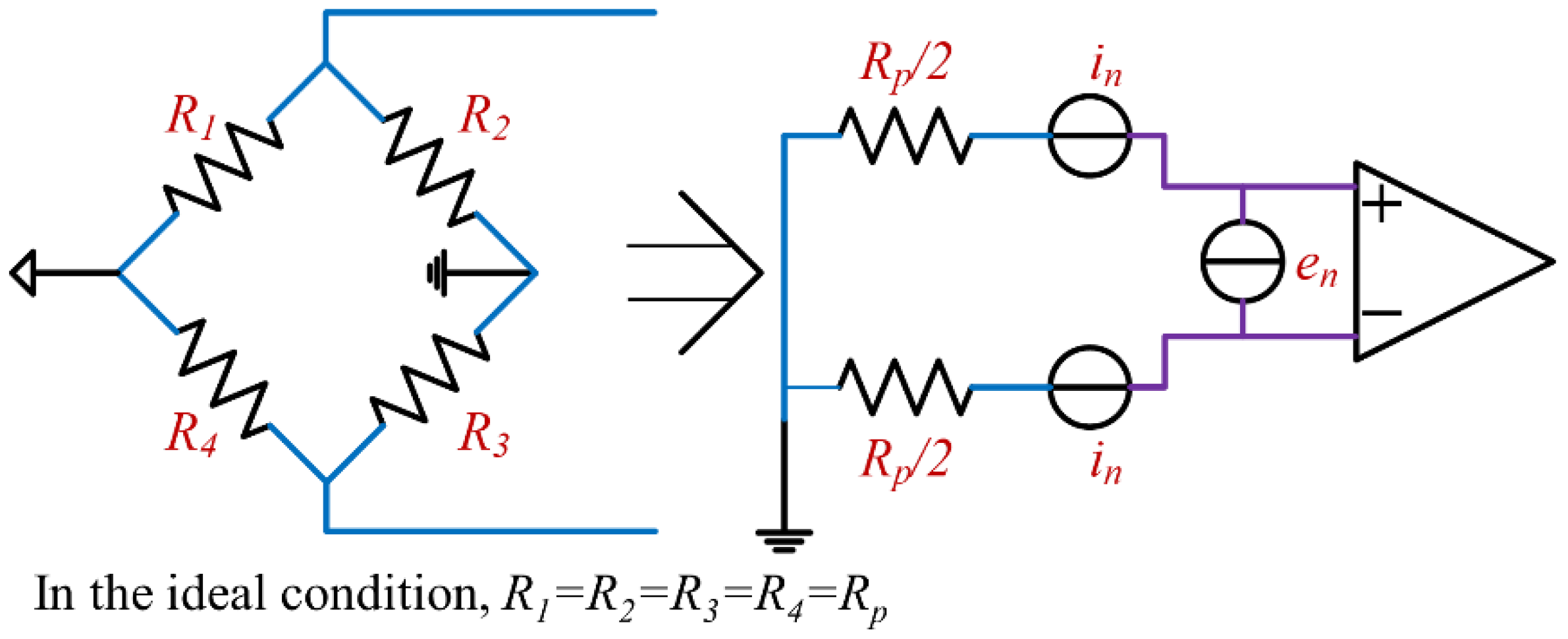
3.1. Electrical Noise
3.2. Mechanical-Thermal Noise
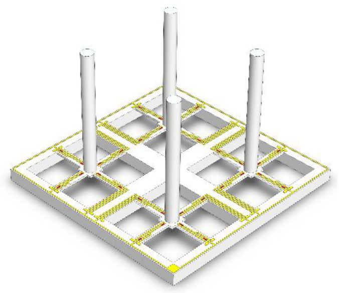
3.3. Noise Suppression by FUVH
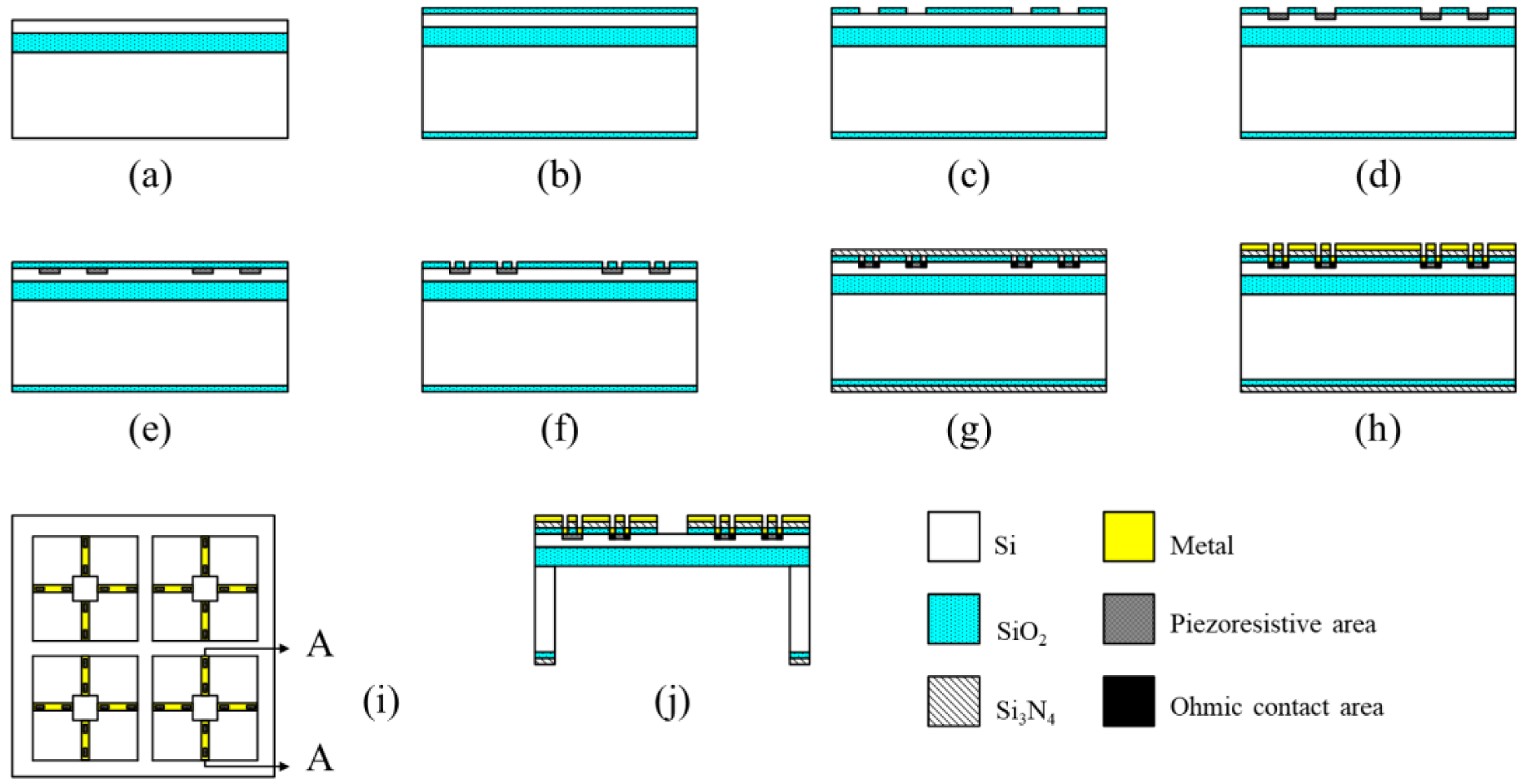
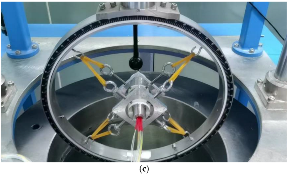
4. Experimental Program
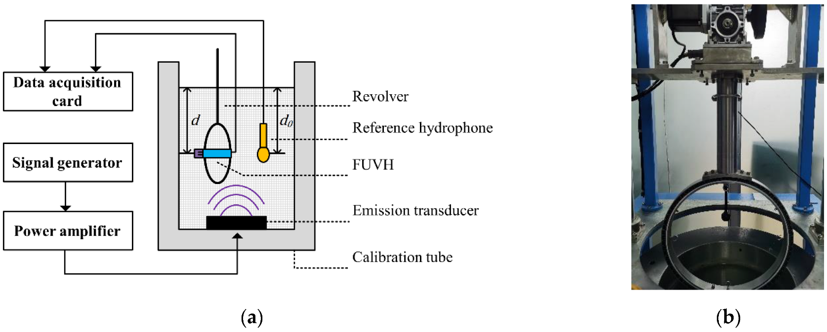
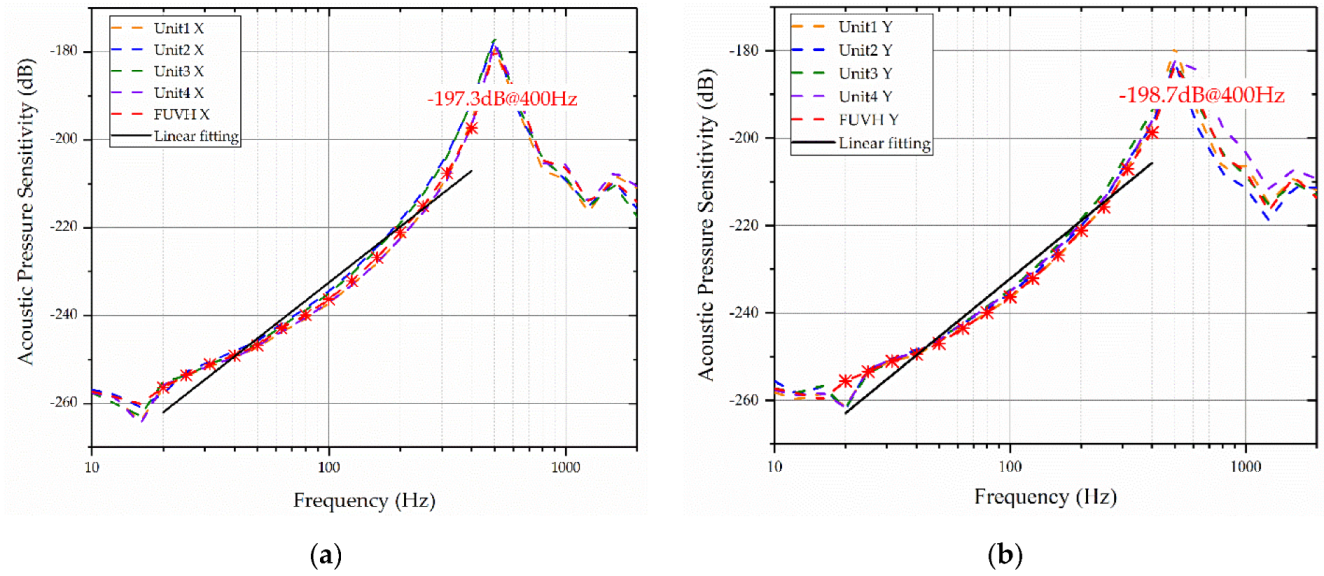
4.1. Sensitivity Test
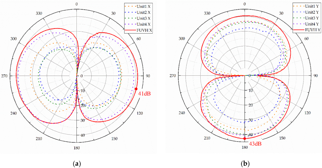
4.2. Directivity Pattern Test
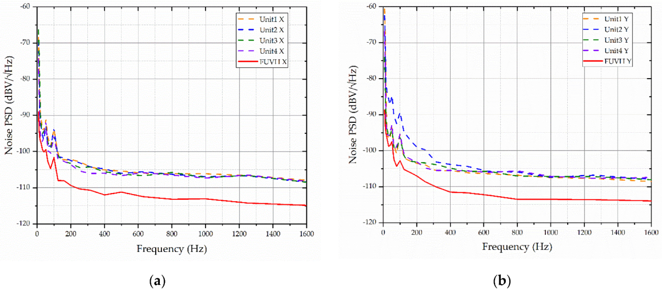
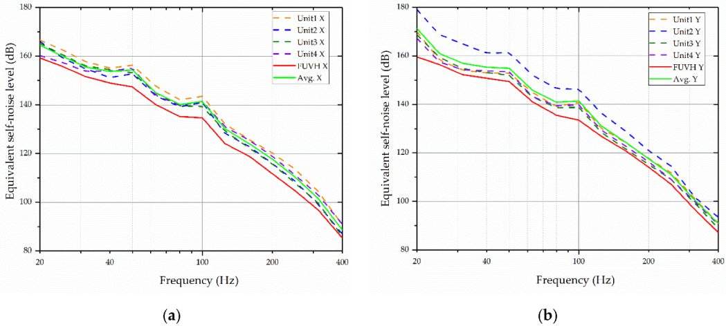
4.3. Self-Noise Test
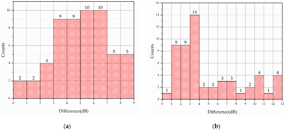
5. Results and Analysis
6. Discussion
Author Contributions
Funding
Conflicts of Interest
References
- Melnichenko, O.; Hacker, P.; Müller, V. Observations of Mesoscale Eddies in Satellite SSS and Inferred Eddy Salt Transport. Remote Sens. 2021, 13, 315. [Google Scholar] [CrossRef]
- Wang, R.; Qiao, Q.; Yang, S.; Kong, X.; Liu, G.; Chen, X.; Yang, H.; Song, D.; Jia, L.; Cui, J.; et al. High-Sensitivity MEMS Shear Probe for Autonomous Profiling Observation of Marine Turbulence. Remote Sens. 2022, 14, 5004. [Google Scholar] [CrossRef]
- Zhu, S.; Zhang, G.; Wu, D.; Liang, X.; Zhang, Y.; Lv, T.; Liu, Y.; Chen, P.; Zhang, W. Research on Direction of Arrival Estimation Based on Self-Contained MEMS Vector Hydrophone. Micromachines 2022, 13, 236. [Google Scholar] [CrossRef]
- Li, B.; Wang, L. An Intelligent Subsurface Buoy Design for Measuring Ocean Ambient Noise. Adv. Ocean Acoust. 2012, 1495, 528–535. [Google Scholar]
- Saheban, H.; Kordrostami, Z. Hydrophones, fundamental features, design considerations, and various structures: A review. Sens. Actuators A Phys. 2021, 329, 112790. [Google Scholar] [CrossRef]
- Liu, Y.; Wang, R.; Zhang, G.; Du, J.; Zhao, L.; Xue, C.; Zhang, W.; Liu, J. “Lollipop-shaped” high-sensitivity Microelectromechanical Systems vector hydrophone based on Parylene encapsulation. J. Appl. Phys. 2015, 118, 044501. [Google Scholar] [CrossRef]
- Xu, W.; Liu, Y.; Zhang, G.; Wang, R.; Xue, C.; Zhang, W.; Liu, J. Development of cup-shaped micro-electromechanical systems-based vector hydrophone. J. Appl. Phys. 2016, 120, 124502. [Google Scholar] [CrossRef]
- Wang, R.; Liu, Y.; Xu, W.; Bai, B.; Zhang, G.; Liu, J.; Xiong, J.; Zhang, W.; Xue, C.; Zhang, B. A ‘fitness-wheel-shaped’ MEMS vector hydrophone for 3D spatial acoustic orientation. J. Micromech. Microeng. 2017, 27, 045015. [Google Scholar] [CrossRef]
- Xu, Q.; Zhang, G.; Ding, J.; Wang, R.; Pei, Y.; Ren, Z.; Shang, Z.; Xue, C.; Zhang, W. Design and implementation of two-component cilia cylinder MEMS vector hydrophone. Sens. Actuators A Phys. 2018, 277, 142–149. [Google Scholar] [CrossRef]
- Chen, P.; Zhang, G.; Yang, X.; Ji, S.; Liang, X.; Lv, T.; Zhang, X.; Zhu, S.; Shang, Z.; Zhang, W. Design and realization of sculpture-shaped ciliary MEMS vector hydrophone. Sens. Actuators A Phys. 2021, 331, 112575. [Google Scholar] [CrossRef]
- Wang, R.; Shen, W.; Zhang, W.; Song, J.; Li, N.; Liu, M.; Zhang, G.; Xue, C.; Zhang, W. Design and implementation of a jellyfish otolith-inspired MEMS vector hydrophone for low-frequency detection. Microsyst. Nanoeng. 2021, 7, 1. [Google Scholar] [CrossRef]
- Zhang, G.; Ding, J.; Xu, W.; Liu, Y.; Wang, R.; Han, J.; Bai, B.; Xue, C.; Liu, J.; Zhang, W. Design and optimization of stress centralized MEMS vector hydrophone with high sensitivity at low frequency. Mech. Syst. Signal Process. 2018, 104, 607–618. [Google Scholar] [CrossRef]
- Song, J.; He, C.; Wang, R.; Xue, C.; Zhang, W. A Mathematical Model of a Piezo-Resistive Eight-Beam Three-Axis Accelerometer with Simulation and Experimental Validation. Sensors 2018, 18, 3641. [Google Scholar] [CrossRef] [Green Version]
- Liu, M.; Zhang, G.; Song, X.; Liu, Y.; Zhang, W. Design of the Monolithic Integrated Array MEMS Hydrophone. IEEE Sens. J. 2016, 16, 989–995. [Google Scholar]
- Zhang, X.; Shang, Z.; Ji, S.; Zhang, G. Influence of array elements’ consistency on SNR of hydrophone array. J. Meas. Sci. Instrum. 2019, 10, 5. [Google Scholar]
- Zhang, X.; Shen, N.; Xu, Q.; Pei, Y.; Lian, Y.; Wang, W.; Zhang, G.; Zhang, W. Design and implementation of anulus-shaped ciliary structure for four-unit MEMS vector hydrophone. Int. J. Metrol. Qual. Eng. 2021, 12, 4. [Google Scholar] [CrossRef]
- Petrov, V.V. Use of a Combined Receiver as a Pressure Hydrophone for Increased Noise Suppression. Meas. Tech. 2019, 62, 460–464. [Google Scholar] [CrossRef]
- Tang, Y.-H.; Zheng, Z.; Xie, S.-M.; Huang, L.; Jiang, H.-B. Thermoacoustic imaging based on noise suppression of multi-channel amplifier and additive circuit. Acta Phys. Sin. 2020, 69, 240701. [Google Scholar] [CrossRef]
- Yang, D.; Yang, L.; Chen, X.; Qu, M.; Zhu, K.; Ding, H.; Li, D.; Bai, Y.; Ling, J.; Xu, J.; et al. A piezoelectric AlN MEMS hydrophone with high sensitivity and low noise density. Sens. Actuators A Phys. 2021, 318, 112493. [Google Scholar] [CrossRef]
- Chen, S.; Xue, C.; Zhang, W.; Xiong, J.; Zhang, B.; Hu, J. A new type of MEMS two axis accelerometer based on Silicon. In Proceedings of the 2008 3rd IEEE International Conference on Nano/Micro Engineered and Molecular Systems, Sanya, China, 6–9 January 2008. [Google Scholar]
- Krishnakumar, R.; Ramesh, R. A Method and an Experimental Setup for Measuring the Self-Noise of Piezoelectric Hydrophones. IEEE Trans. Ultrason. Ferroelectr. Freq. Control 2020, 67, 413–421. [Google Scholar] [CrossRef]
- Gabrielson, T.B. Mechanical-thermal Noise in Micromachined Acoustic and Vibration Sensors. IEEE Trans. Electron. Devices 1993, 40, 903–909. [Google Scholar] [CrossRef] [Green Version]
- Gabrielson, T.B. Fundamental Noise Limits for Miniature Acoustic and Vibration Sensors. J. Vib. Acoust. 1995, 117, 405–410. [Google Scholar] [CrossRef]
- Fang, E.; Hong, L.; Yang, D. Self-noise analysis of the MEMS hydrophone. J. Harbin Eng. Univ. 2014, 35, 4. [Google Scholar]
- Durdaut, P.; Salzer, S.; Reermann, J.; Robisch, V.; Hayes, P.; Piorra, A.; Meyners, D.; Quandt, E.; Schmidt, G.; Knochel, R.; et al. Thermal-Mechanical Noise in Resonant Thin-Film Magnetoelectric Sensors. IEEE Sens. J. 2017, 17, 2338–2348. [Google Scholar] [CrossRef]
- Lin, R.M.; Wang, W.J. Structural dynamics of microsystems—Current state of research and future directions. Mech. Syst. Signal Process. 2006, 20, 1015–1043. [Google Scholar] [CrossRef]
- Kongthon, J.; McKay, B.; Iamratanakul, D.; Oh, K.; Chung, J.-H.; Riley, J.; Devasia, S. Added-Mass Effect in Modeling of Cilia-Based Devices for Microfluidic Systems. J. Vib. Acoust. 2010, 132, 024501. [Google Scholar] [CrossRef]
- Wang, R.; Liu, Y.; Bai, B.; Guo, N.; Guo, J.; Wang, X.; Liu, M.; Zhang, G.; Zhang, B.; Xue, C.; et al. Wide-frequency-bandwidth whisker-inspired MEMS vector hydrophone encapsulated with parylene. J. Phys. D Appl. Phys. 2016, 49, 07LT02. [Google Scholar] [CrossRef]
- Besson, O.; Kraut, S.; Scharf, L.L. Detection of an unknown rank-one component in white noise. IEEE Trans. Signal Process. 2006, 54, 2835–2839. [Google Scholar] [CrossRef] [Green Version]
- Zhang, G.; Wang, P.; Guan, L.; Xiong, J.; Zhang, W. Improvement of the MEMS bionic vector hydrophone. Microelectron. J. 2011, 42, 815–819. [Google Scholar] [CrossRef]
- Guo, J.; Zhang, G.; Wang, X.; Zhang, W. Analysis for microstructure of MEMS bionic vector hydrophone. High Power Laser Part. Beams 2015, 27, 024125. [Google Scholar] [CrossRef]
- Liang, X.; Lv, T.; Ji, S.; Chen, P.; Zhang, Y.; Li, C.; Zhu, S.; Zhang, G.; Zhang, W.; Wang, R. The Influence of Ambient Temperature on the Sensitivity of MEMS Vector Hydrophone. IEEE Sens. J. 2021, 21, 17678–17685. [Google Scholar] [CrossRef]
- Xue, C.; Chen, S.; Zhang, W.; Zhang, B.; Zhang, G.; Qiao, H. Design, fabrication, and preliminary characterization of a novel MEMS bionic vector hydrophone. Microelectron. J. 2007, 38, 1021–1026. [Google Scholar] [CrossRef]
- Liu, G.; Cao, W.; Zhang, G.; Wang, Z.; Tan, H.; Miao, J.; Li, Z.; Zhang, W.; Wang, R. Design and Simulation of Flexible Underwater Acoustic Sensor Based on 3D Buckling Structure. Micromachines 2021, 12, 1536. [Google Scholar] [CrossRef]
- Zhang, G.; Zhang, L.; Ji, S.; Yang, X.; Wang, R.; Zhang, W.; Yang, S. Design and Implementation of a Composite Hydrophone of Sound Pressure and Sound Pressure Gradient. Micromachines 2021, 12, 939. [Google Scholar] [CrossRef]
- Li, Z.; Chen, H. Method for measuring self-noise of vector hydrophones. J. Mar. Sci. Appl. 2017, 16, 370–374. [Google Scholar] [CrossRef]


| Parameter | Description | Value (μm) |
|---|---|---|
| beam length | L | 1000 |
| support block’s side length | 2a | 600 |
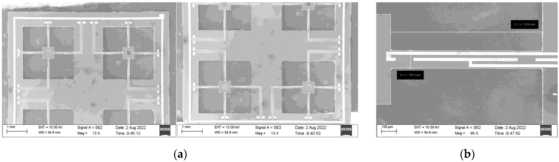
| beam width | b | 120 |
| beam thickness | t | 40 |
| cilium height | H | 8000 |
Publisher’s Note: MDPI stays neutral with regard to jurisdictional claims in published maps and institutional affiliations. |
© 2022 by the authors. Licensee MDPI, Basel, Switzerland. This article is an open access article distributed under the terms and conditions of the Creative Commons Attribution (CC BY) license (https://creativecommons.org/licenses/by/4.0/).
Share and Cite
Tan, H.; Liu, G.; Li, H.; Zhang, G.; Cui, J.; Yang, Y.; He, C.; Jia, L.; Zhang, W.; Wang, R. Research on Self-Noise Suppression of Marine Acoustic Sensor Arrays. Remote Sens. 2022, 14, 6186. https://doi.org/10.3390/rs14246186
Tan H, Liu G, Li H, Zhang G, Cui J, Yang Y, He C, Jia L, Zhang W, Wang R. Research on Self-Noise Suppression of Marine Acoustic Sensor Arrays. Remote Sensing. 2022; 14(24):6186. https://doi.org/10.3390/rs14246186
Chicago/Turabian StyleTan, Haoyu, Guochang Liu, Haoxuan Li, Guojun Zhang, Jiangong Cui, Yuhua Yang, Changde He, Licheng Jia, Wendong Zhang, and Renxin Wang. 2022. "Research on Self-Noise Suppression of Marine Acoustic Sensor Arrays" Remote Sensing 14, no. 24: 6186. https://doi.org/10.3390/rs14246186