


A Sentinel-2 Based Multi-Temporal Monitoring Framework for Wind and Bark Beetle Detection and Damage Mapping


Abstract
:
1. Introduction
2. Materials and Methods
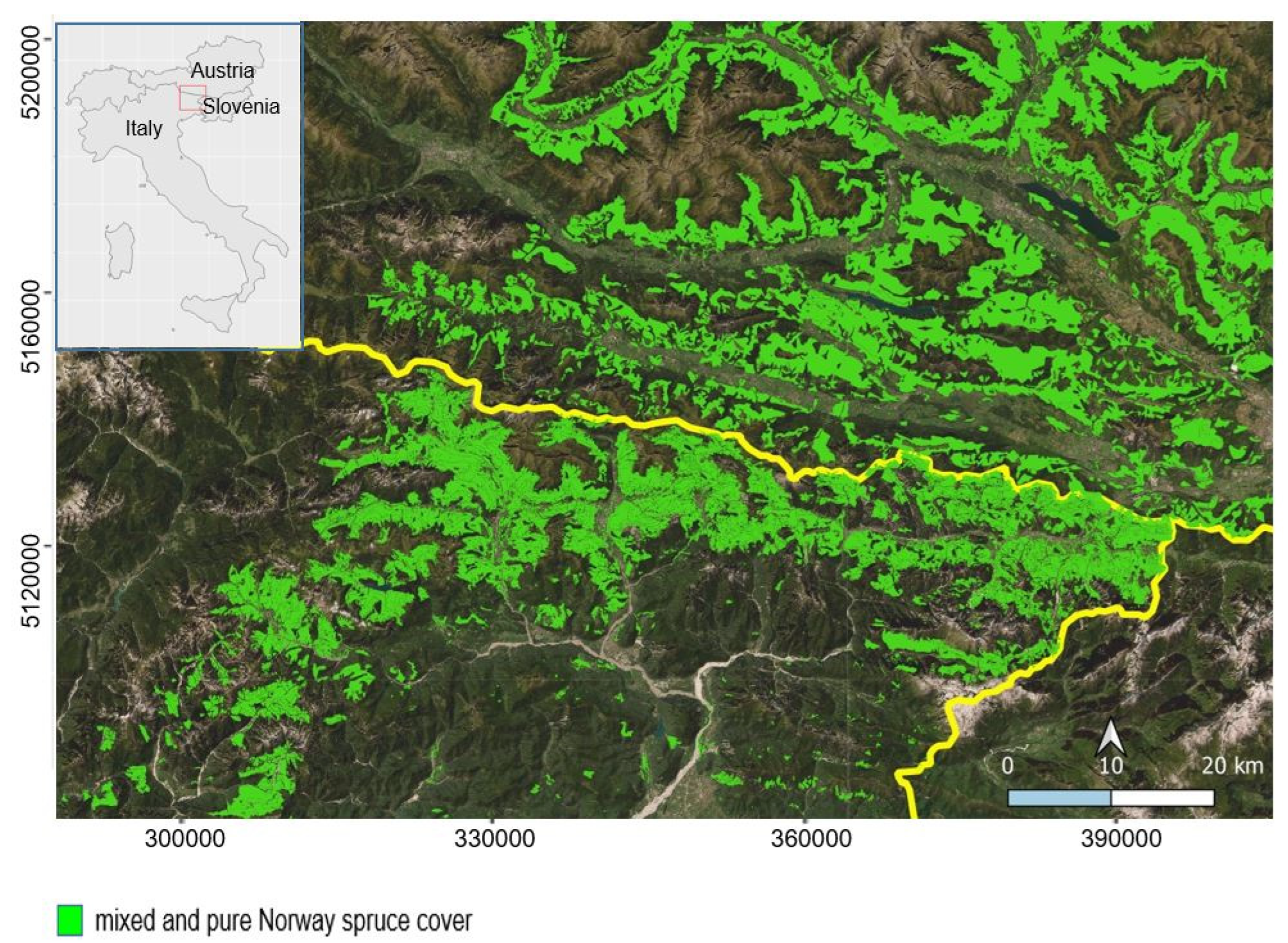
2.1. Study Area
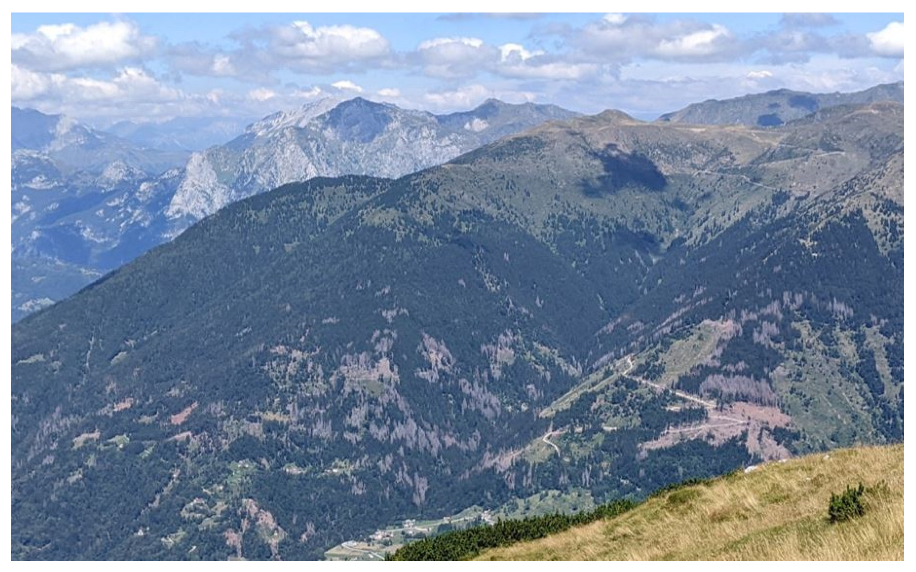
The Vaia Storm
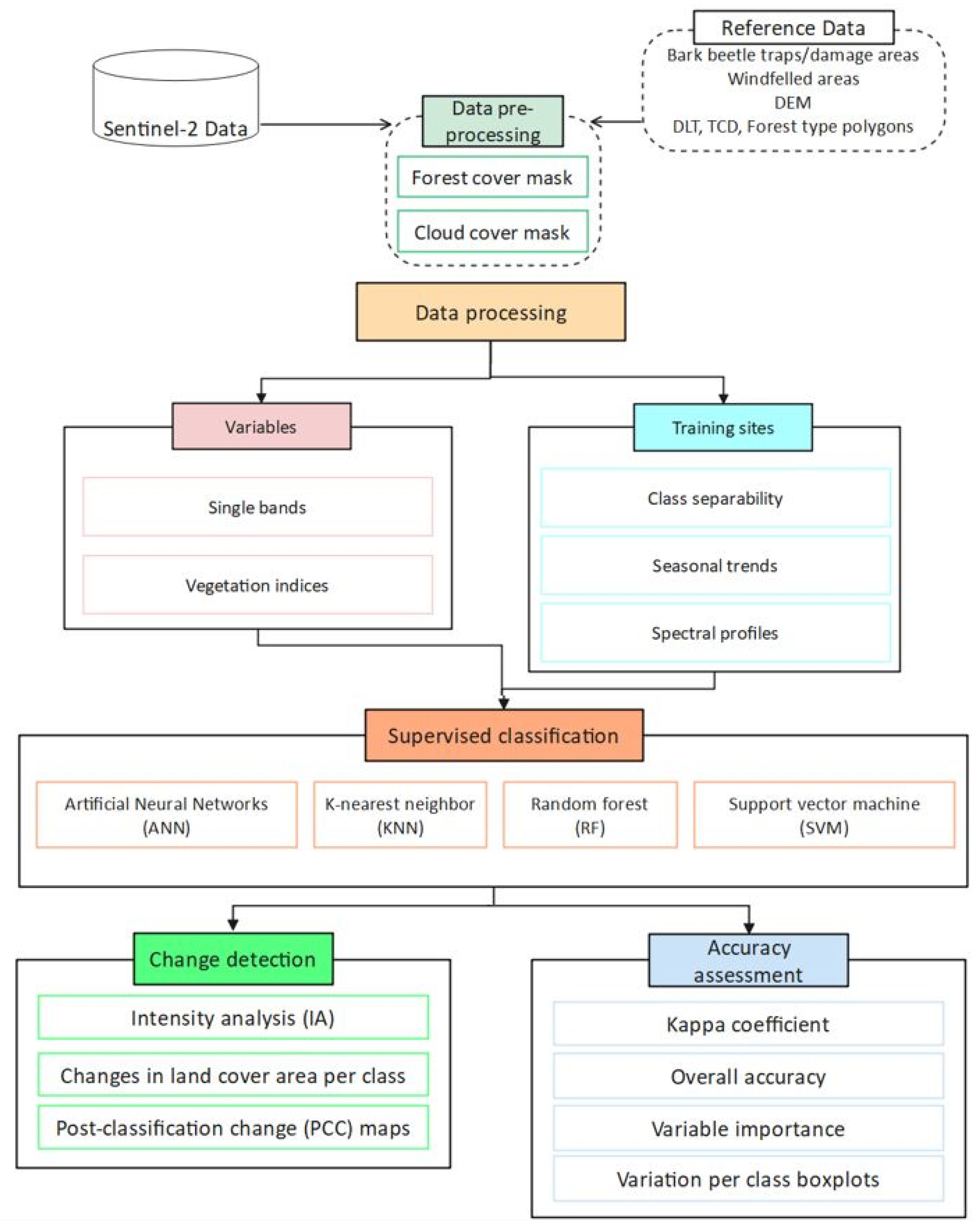
2.2. Data
2.3. Methods
2.3.1. Single Bands and Vegetation Indices
2.3.2. Supervised Classification of Multi-Temporal Imagery
2.3.3. Post-Classification Forest-Cover Change Detection
3. Results
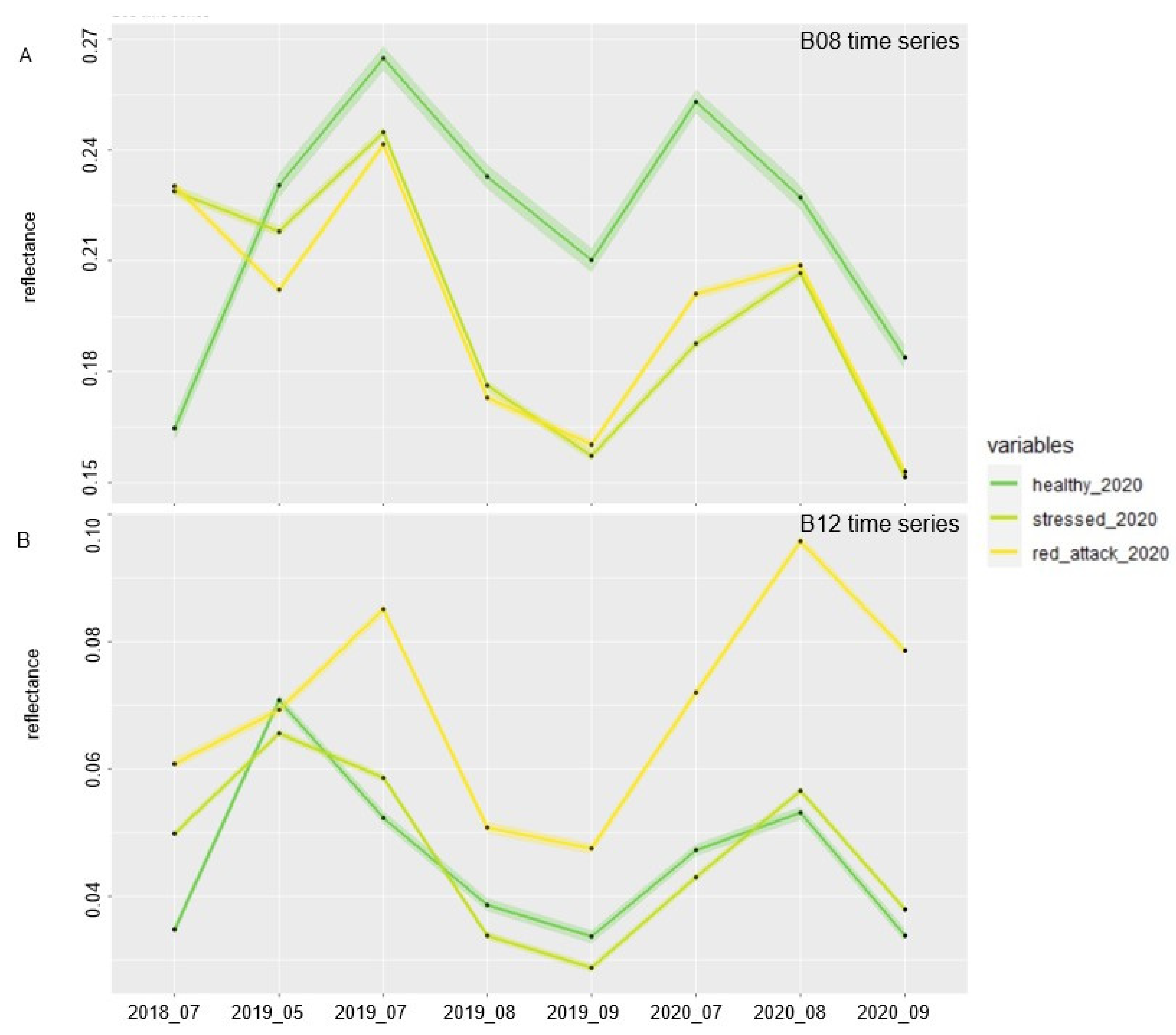
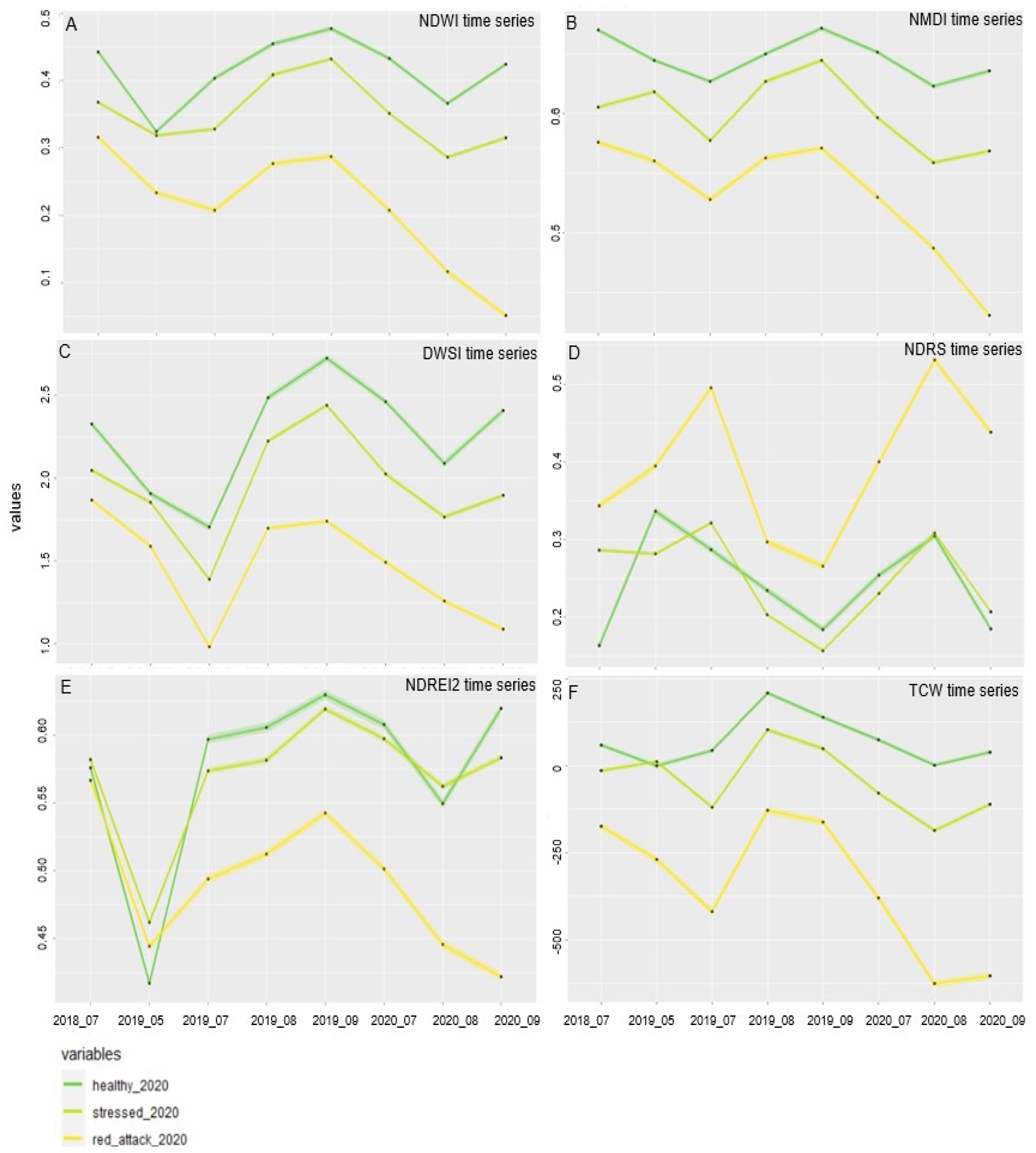
3.1. Single Bands and Vegetation Indices Reflectance Values
3.2. Supervised Classification
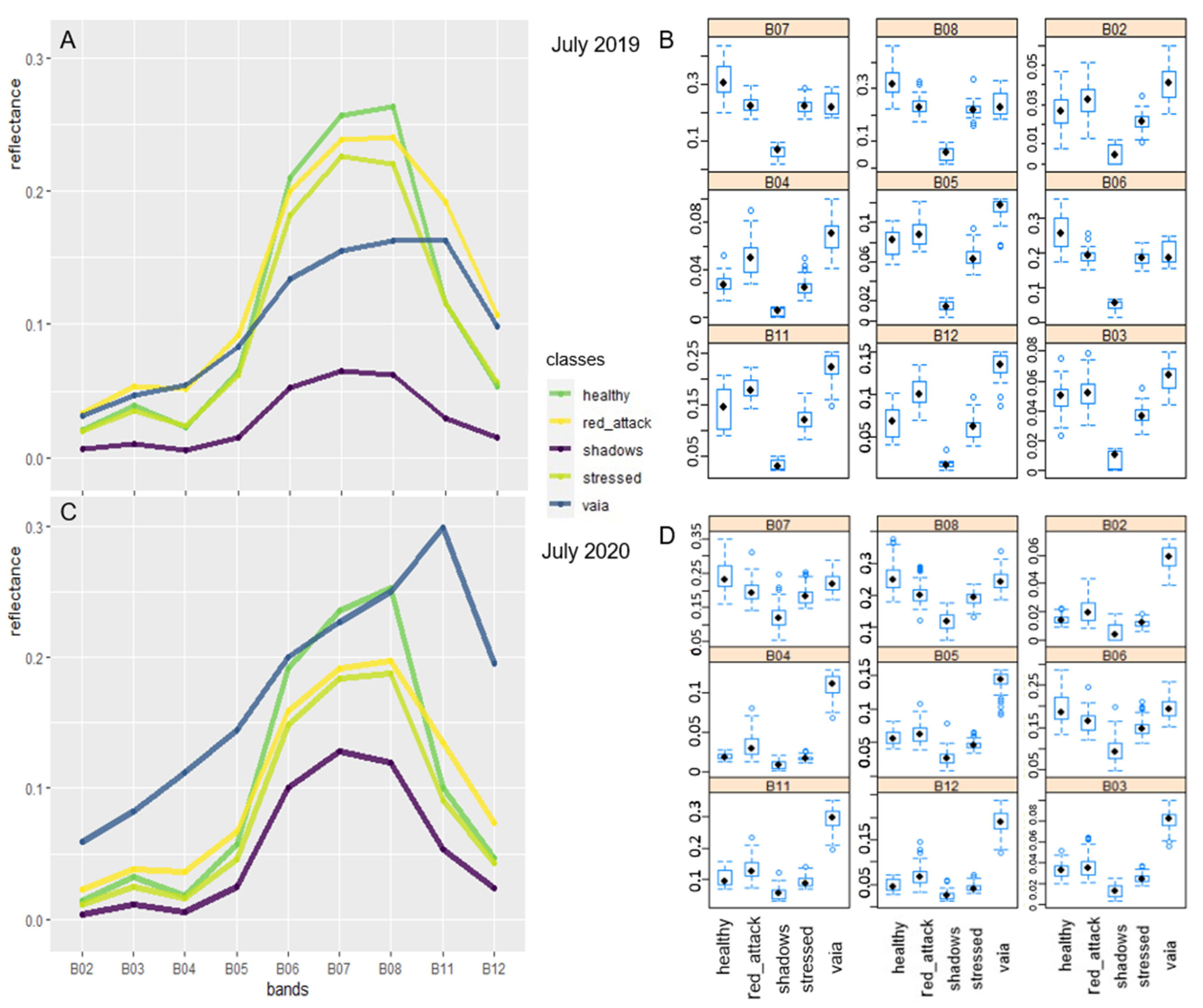
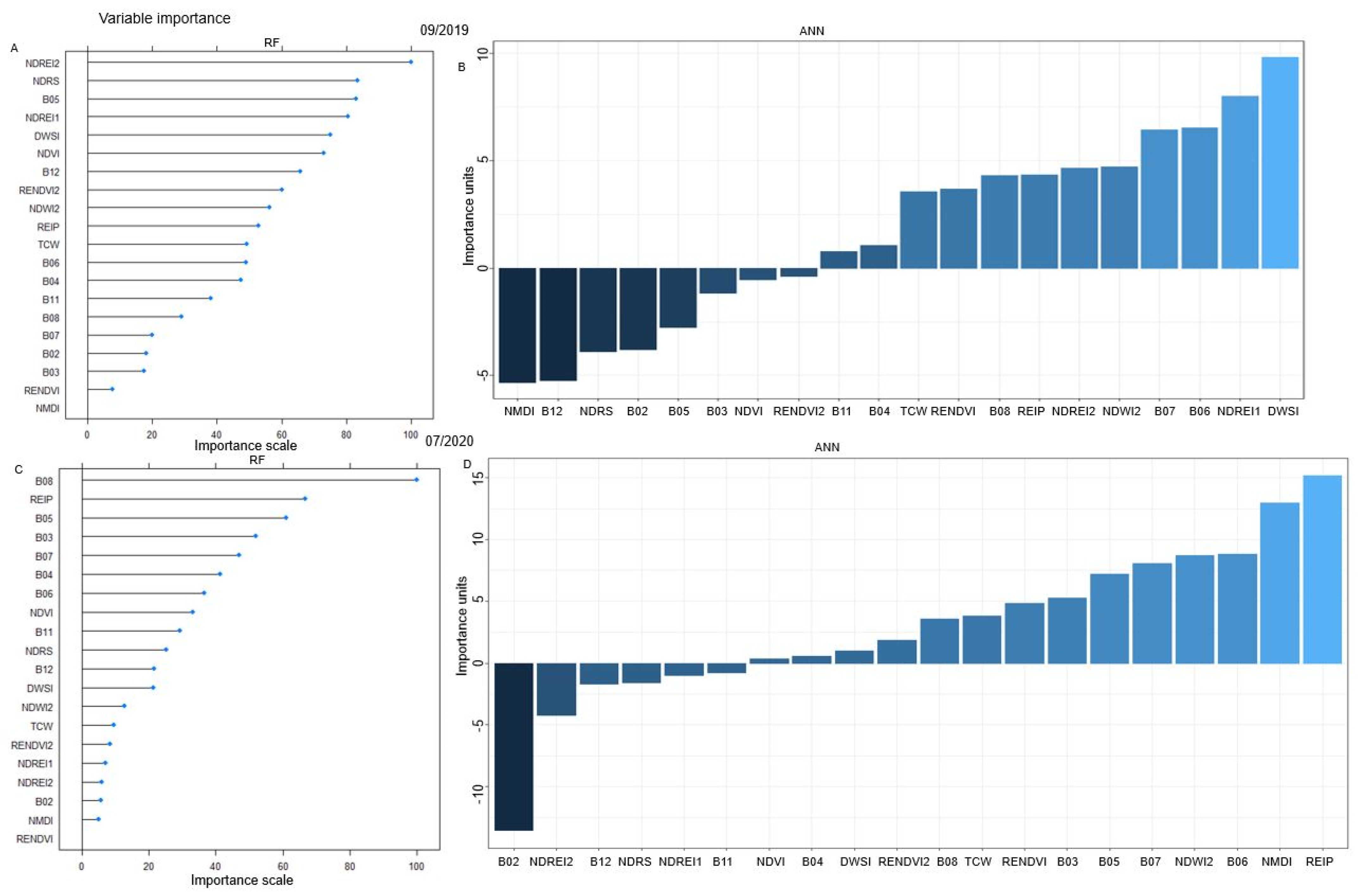
3.2.1. Spectral Signatures
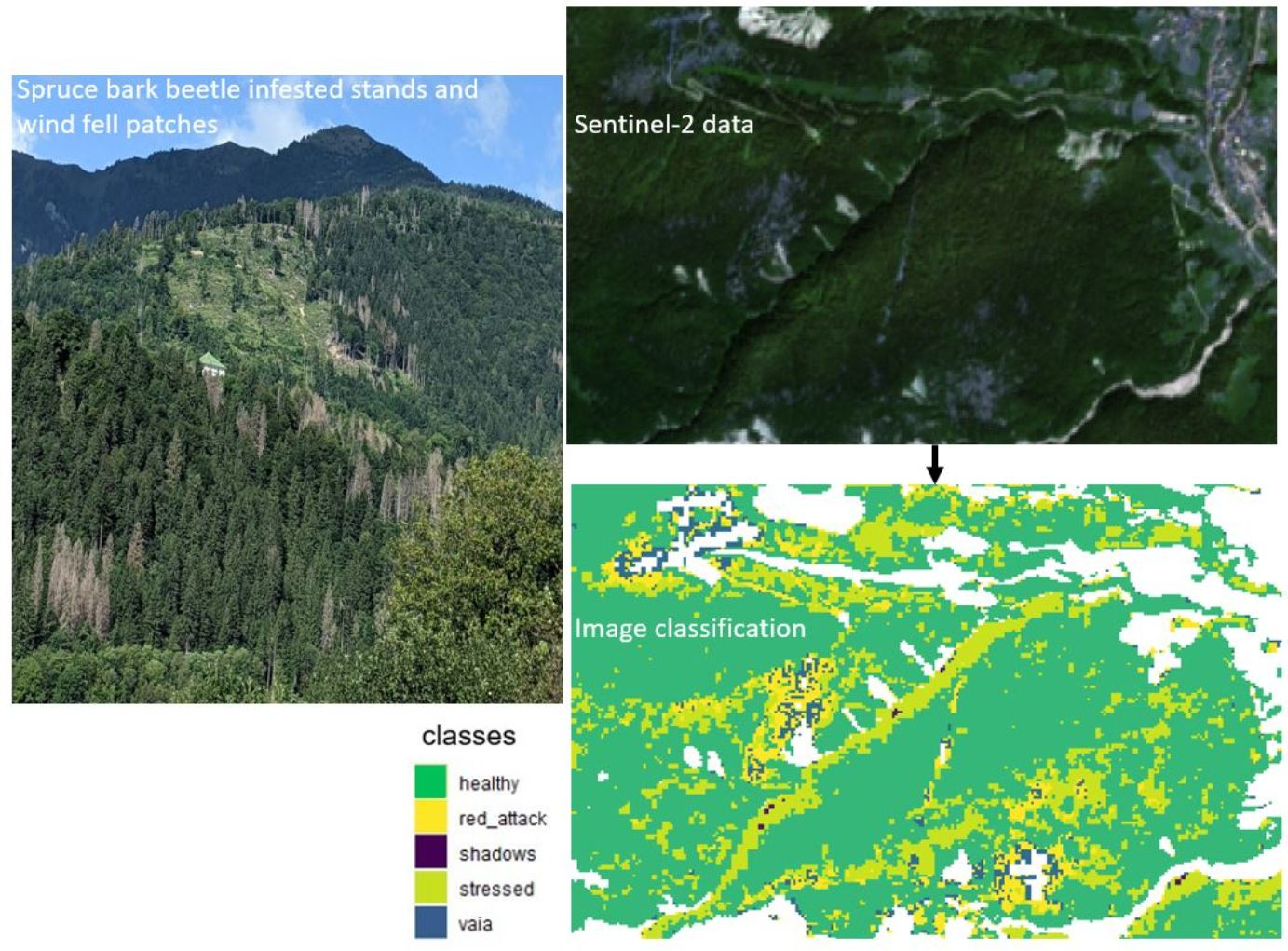
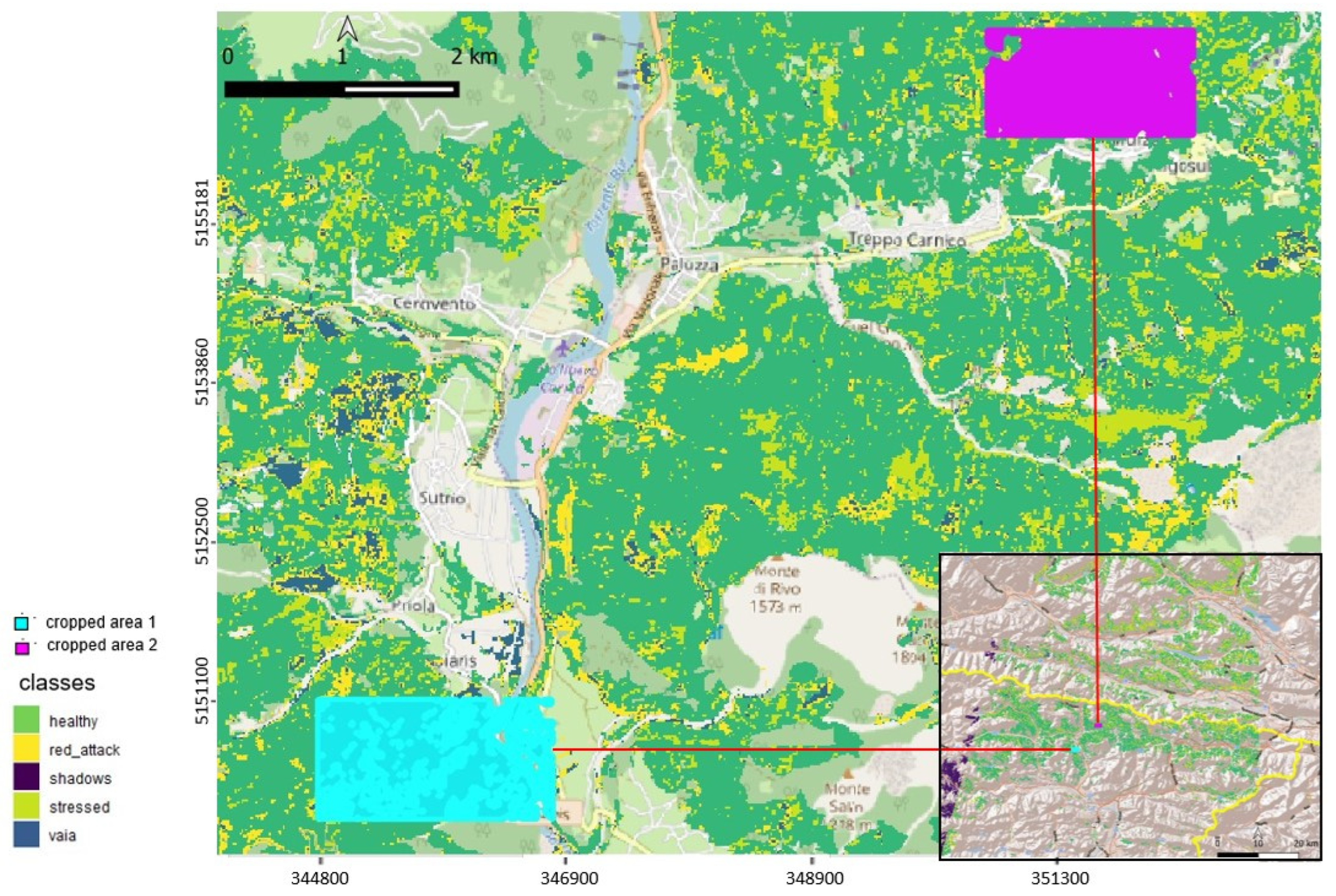
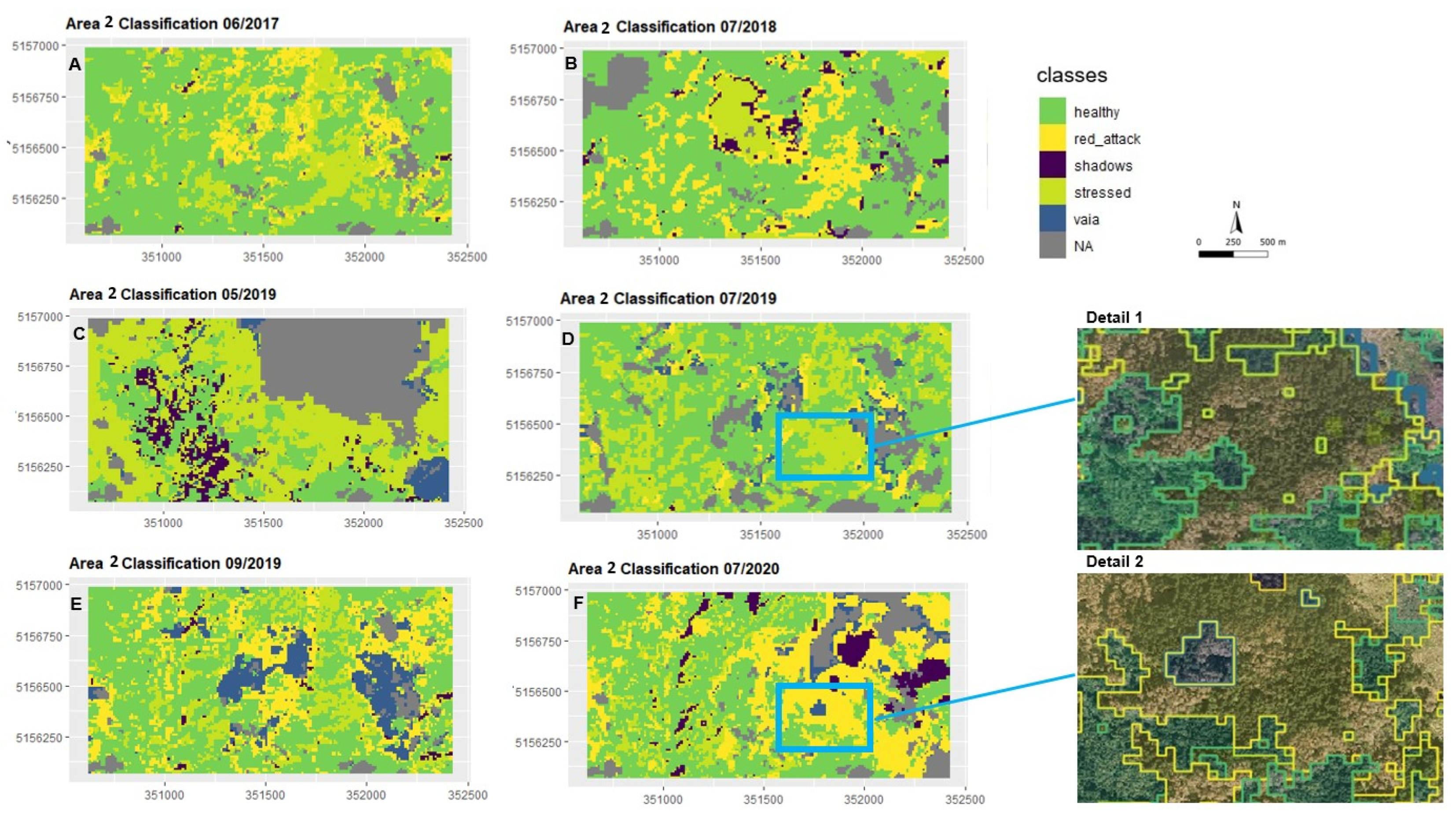
3.2.2. Maps of Damage
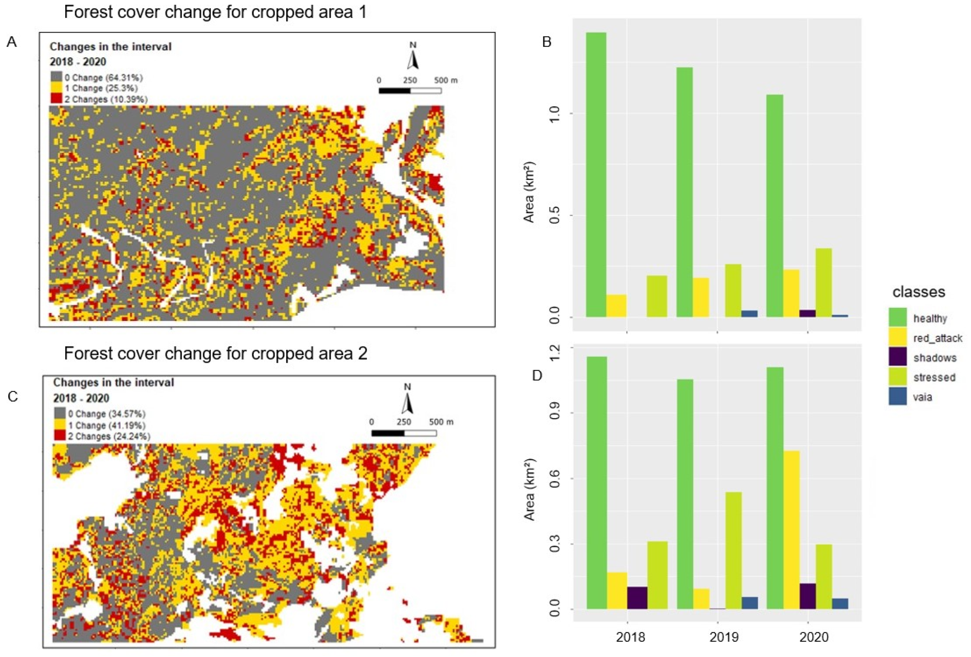
3.3. Post-Classification Change Detection
4. Discussion
5. Conclusions
Author Contributions
Funding
Data Availability Statement
Acknowledgments
Conflicts of Interest
Appendix A

| 06/2017 RF | ||||||
| Confusion Matrix and Statistics | ||||||
| Reference | ||||||
| Prediction | healthy | red_attack | shadows | stressed | ||
| healthy | 24 | 1 | 0 | 0 | ||
| red_attack | 0 | 31 | 0 | 3 | ||
| shadows | 0 | 0 | 26 | 0 | ||
| stressed | 1 | 1 | 0 | 32 | ||
| Overall Statistics | ||||||
| Accuracy | 0.9535 | |||||
| 95% CI | (0.9015, 0.9827) | |||||
| No-Information Rate | 0.2713 | |||||
| p-Value (Acc > NIR) | <2.2 × 10⁻¹⁶ | |||||
| Kappa | 0.9377 | |||||
| 06/2017 ANN | ||||||
| Confusion Matrix and Statistics | ||||||
| Reference | ||||||
| Prediction | healthy | red_attack | shadows | stressed | ||
| healthy | 33 | 1 | 0 | 1 | ||
| red_attack | 0 | 31 | 0 | 6 | ||
| shadows | 0 | 0 | 26 | 0 | ||
| stressed | 2 | 1 | 0 | 28 | ||
| Overall Statistics | ||||||
| Accuracy | 0.9147 | |||||
| 95% CI | (0.8525, 0.9567) | |||||
| No-Information Rate | 0.2713 | |||||
| p-Value (Acc > NIR) | <2.2 × 10⁻¹⁶ | |||||
| Kappa | 0.8859 | |||||
| 07/2018 RF | ||||||
| Confusion Matrix and Statistics | ||||||
| Reference | ||||||
| Prediction | healthy | red_attack | shadows | stressed | ||
| healthy | 23 | 1 | 0 | 0 | ||
| red_attack | 0 | 24 | 0 | 1 | ||
| shadows | 0 | 0 | 23 | 0 | ||
| stressed | 4 | 2 | 0 | 26 | ||
| Overall Statistics | ||||||
| Accuracy | 0.9231 | |||||
| 95% CI | (0.854, 0.9662) | |||||
| No-Information Rate | 0.2596 | |||||
| p-Value (Acc > NIR) | <2.2 × 10⁻¹⁶ | |||||
| Kappa | 0.8973 | |||||
| 07/2018 ANN | ||||||
| Confusion Matrix and Statistics | ||||||
| Reference | ||||||
| Prediction | healthy | red_attack | shadows | stressed | ||
| healthy | 26 | 0 | 0 | 3 | ||
| red_attack | 0 | 26 | 1 | 0 | ||
| shadows | 0 | 0 | 22 | 0 | ||
| stressed | 1 | 1 | 0 | 24 | ||
| Overall Statistics | ||||||
| Accuracy | 0.9423 | |||||
| 95% CI | (0.8787, 0.9785) | |||||
| No-Information Rate | 0.2596 | |||||
| p-Value (Acc > NIR) | <2.2 × 10⁻¹⁶ | |||||
| Kappa | 0.9229 | |||||
| 05/2019 RF | ||||||
| Confusion Matrix and Statistics | ||||||
| Reference | ||||||
| Prediction | healthy | shadows | stressed | vaia | ||
| healthy | 23 | 0 | 1 | 0 | ||
| shadows | 0 | 19 | 0 | 0 | ||
| stressed | 0 | 0 | 23 | 0 | ||
| vaia | 0 | 0 | 0 | 19 | ||
| Overall Statistics | ||||||
| Accuracy | 0.9882 | |||||
| 95% CI | (0.9362, 0.9997) | |||||
| No-Information Rate | 0.2824 | |||||
| p-Value (Acc > NIR) | <2.2 × 10⁻¹⁶ | |||||
| Kappa | 0.9843 | |||||
| 05/2019 ANN | ||||||
| Confusion Matrix and Statistics | ||||||
| Reference | ||||||
| Prediction | healthy | shadows | stressed | vaia | ||
| healthy | 23 | 0 | 0 | 0 | ||
| shadows | 0 | 19 | 0 | 0 | ||
| stressed | 0 | 0 | 24 | 0 | ||
| vaia | 0 | 0 | 0 | 19 | ||
| Overall Statistics | ||||||
| Accuracy | 1 | |||||
| 95% CI | (0.9575, 1) | |||||
| No-Information Rate | 0.2824 | |||||
| p-Value (Acc > NIR) | <2.2 × 10⁻¹⁶ | |||||
| Kappa | 1 | |||||
| 07/2019 RF | ||||||
| Confusion Matrix and Statistics | ||||||
| Reference | ||||||
| Prediction | healthy | red_attack | shadows | stressed | vaia | |
| healthy | 45 | 0 | 0 | 0 | 0 | |
| red_attack | 0 | 23 | 0 | 2 | 5 | |
| shadows | 0 | 0 | 10 | 0 | 0 | |
| stressed | 0 | 3 | 0 | 59 | 0 | |
| vaia | 0 | 2 | 0 | 0 | 8 | |
| Overall Statistics | ||||||
| Accuracy | 0.9236 | |||||
| 95% CI | (0.8703, 0.9588) | |||||
| No-Information Rate | 0.3885 | |||||
| p-Value (Acc > NIR) | <2.2 × 10⁻¹⁶ | |||||
| Kappa | 0.894 | |||||
| 07/2019 ANN | ||||||
| Confusion Matrix and Statistics | ||||||
| Reference | ||||||
| Prediction | healthy | red_attack | shadows | stressed | vaia | |
| healthy | 27 | 1 | 0 | 1 | 0 | |
| red_attack | 0 | 21 | 0 | 1 | 2 | |
| shadows | 0 | 0 | 11 | 0 | 0 | |
| stressed | 2 | 3 | 0 | 32 | 1 | |
| vaia | 0 | 3 | 0 | 0 | 13 | |
| Overall Statistics | ||||||
| Accuracy | 0.8814 | |||||
| 95% CI | (0.809, 0.9366) | |||||
| No-Information Rate | 0.2881 | |||||
| p-Value (Acc > NIR) | <2.2 × 10⁻¹⁶ | |||||
| Kappa | 0.8462 | |||||
| 09/2019 RF | ||||||
| Confusion Matrix and Statistics | ||||||
| Reference | ||||||
| Prediction | healthy | red_attack | shadows | stressed | vaia | |
| healthy | 25 | 0 | 0 | 1 | 0 | |
| red_attack | 1 | 17 | 0 | 2 | 1 | |
| shadows | 0 | 0 | 3 | 0 | 0 | |
| stressed | 1 | 0 | 0 | 24 | 0 | |
| vaia | 0 | 1 | 0 | 0 | 20 | |
| Overall Statistics | ||||||
| Accuracy | 0.9271 | |||||
| 95% CI | (0.8555, 0.9702) | |||||
| No-Information Rate | 0.2812 | |||||
| p-Value (Acc > NIR) | <2.2 × 10⁻¹⁶ | |||||
| Kappa | 0.9042 | |||||
| 09/2019 ANN | ||||||
| Confusion Matrix and Statistics | ||||||
| Reference | ||||||
| Prediction | healthy | red_attack | shadows | stressed | vaia | |
| healthy | 24 | 4 | 0 | 2 | 0 | |
| red_attack | 2 | 12 | 0 | 3 | 0 | |
| shadows | 0 | 0 | 3 | 0 | 0 | |
| stressed | 1 | 1 | 0 | 21 | 0 | |
| vaia | 0 | 1 | 0 | 1 | 21 | |
| Overall Statistics | ||||||
| Accuracy | 0.8438 | |||||
| 95% CI | (0.7554, 0.9098) | |||||
| No-Information Rate | 0.2812 | |||||
| p-Value (Acc > NIR) | <2.2 × 10⁻¹⁶ | |||||
| Kappa | 0.7939 | |||||
| 07/2020 RF | ||||||
| Confusion Matrix and Statistics | ||||||
| Reference | ||||||
| Prediction | healthy | red_attack | shadows | stressed | vaia | |
| healthy | 31 | 0 | 0 | 3 | 0 | |
| red_attack | 0 | 28 | 0 | 2 | 0 | |
| shadows | 0 | 0 | 43 | 2 | 0 | |
| stressed | 4 | 7 | 0 | 28 | 0 | |
| vaia | 0 | 0 | 0 | 0 | 7 | |
| Overall Statistics | ||||||
| Accuracy | 0.8839 | |||||
| 95% CI | (0.8227, 0.9297) | |||||
| No-Information Rate | 0.2774 | |||||
| p-Value (Acc > NIR) | <2.2 × 10⁻¹⁶ | |||||
| Kappa | 0.8487 | |||||
| 07/2020 ANN | ||||||
| Confusion Matrix and Statistics | ||||||
| Reference | ||||||
| Prediction | healthy | red_attack | shadows | stressed | vaia | |
| healthy | 27 | 0 | 0 | 4 | 0 | |
| red_attack | 1 | 28 | 0 | 6 | 0 | |
| shadows | 0 | 0 | 43 | 6 | 0 | |
| stressed | 7 | 7 | 0 | 19 | 0 | |
| vaia | 0 | 0 | 0 | 0 | 7 | |
| Overall Statistics | ||||||
| Accuracy | 0.8 | |||||
| 95% CI | (0.7283, 0.8599) | |||||
| No-Information Rate | 0.2774 | |||||
| p-Value (Acc > NIR) | <2.2 × 10⁻¹⁶ | |||||
| Kappa | 0.7389 | |||||


References
- Gandhi, K.J.; Hofstetter, R.W. Bark Beetle Management, Ecology and Climate Change, 1st ed.; Academic Press: London, UK, 2021. [Google Scholar]
- Niemann, K.O.; Quinn, G.; Stephen, R.; Visintini, F.; Parton, D. Hyperspectral Remote Sensing of Mountain Pine Beetle with an Emphasis on Previsual Assessment. Can. J. Remote Sens. 2015, 41, 191–202. [Google Scholar] [CrossRef]
- Seidl, R.; Thom, D.; Kautz, M.; Martin-Benito, D.; Peltoniemi, M.; Vacchiano, G.; Wild, J.; Ascoli, D.; Petr, M.; Honkaniemi, J.; et al. Forest disturbances under climate change. Nat. Clim. Chang. 2017, 7, 395–402. [Google Scholar] [CrossRef] [PubMed] [Green Version]
- Huang, J.; Kautz, M.; Trowbridge, A.M.; Hammerbacher, A.; Raffa, K.F.; Adams, H.D.; Goodsman, D.W.; Xu, C.; Meddens, A.J.; Kandasamy, D.; et al. Tree defense and bark beetles in a drying world: Carbon partitioning, functioning and modelling. New Phytol. 2020, 225, 26–36. [Google Scholar] [CrossRef] [PubMed] [Green Version]
- Montzka, C.; Bayat, B.; Tewes, A.; Mengen, D.; Vereecken, H. Sentinel-2 Analysis of Spruce Crown Transparency Levels and Their Environmental Drivers After Summer Drought in the Northern Eifel (Germany). Front. For. Glob. Chang. 2021, 4, 86. [Google Scholar] [CrossRef]
- Morris, J.L.; Cottrell, S.; Fettig, C.J.; Hansen, W.D.; Sherriff, R.L.; Carter, V.A.; Clear, J.L.; Clement, J.; DeRose, R.J.; Hicke, J.A.; et al. Managing bark beetle impacts on ecosystems and society: Priority questions to motivate future research. J. Appl. Ecol. 2017, 54, 750–760. [Google Scholar] [CrossRef]
- Dobor, L.; Hlásny, T.; Zimová, S. Contrasting vulnerability of monospecific and species-diverse forests to wind and bark beetle disturbance: The role of management. Ecol. Evol. 2020, 10, 12233–12245. [Google Scholar] [CrossRef]
- Wermelinger, B. Ecology and management of the spruce bark beetle Ips typographus—A review of recent research. For. Ecol. Manag. 2004, 202, 67–82. [Google Scholar] [CrossRef]
- Niemann, K.O.; Visintini, F. Assessment of Potential for Remote Sensing Detection of Bark Beetle-Infested Areas during Green Attack: A Literature Review; Mountain Pine Beetle Initiative Working Paper 2005-02; Natural Resources Canada, Canadian Forest Service, Pacific Forestry Centre: Victoria, BC, Canada, 2005. [Google Scholar]
- White, J.; Wulder, M.; Brooks, D.; Reich, R.; Wheate, R. Detection of Red Attack Stage Mountain Pine Beetle Infestation with High Spatial Resolution Satellite Imagery. Remote Sens. Environ. 2005, 96, 340–351. [Google Scholar] [CrossRef]
- Wulder, M.A.; Dymond, C.C.; White, J.C.; Leckie, D.G.; Carroll, A.L. Surveying Mountain Pine Beetle Damage of Forests: A Review of Remote Sensing Opportunities. For. Ecol. Manag. 2006, 221, 27–41. [Google Scholar] [CrossRef]
- Hlásny, T.; König, L.; Krokene, P.; Lindner, M.; Montagné-Huck, C.; Müller, J.; Qin, H.; Raffa, K.F.; Schelhaas, M.-J.; Svoboda, M.; et al. Bark Beetle Outbreaks in Europe: State of Knowledge and Ways Forward for Management. Curr. For. Rep. 2021, 7, 138–165. [Google Scholar] [CrossRef]
- Lechner, A.M.; Foody, G.M.; Boyd, D.S. Applications in Remote Sensing to Forest Ecology and Management. One Earth 2020, 2, 405–412. [Google Scholar] [CrossRef]
- Fernandez-Carrillo, A.; Patočka, Z.; Dobrovolný, L.; Franco-Nieto, A.; Revilla-Romero, B. Monitoring Bark Beetle Forest Damage in Central Europe. A Remote Sensing Approach Validated with Field Data. Remote Sens. 2020, 12, 3634. [Google Scholar] [CrossRef]
- Bárta, V.; Lukeš, P.; Homolová, L. Early Detection of Bark Beetle Infestation in Norway Spruce Forests of Central Europe Using Sentinel-2. Int. J. Appl. Earth Obs. Geoinf. 2021, 100, 102335. [Google Scholar] [CrossRef]
- Senf, C.; Seidl, R.; Hostert, P. Remote Sensing of forest insect disturbances: Current state and future directions. Int. J. Appl. Earth Obs. Geoinf. 2017, 60, 49–60. [Google Scholar] [CrossRef] [Green Version]
- Zarco-Tejada, P.J.; Sepulcre-Cantó, G. Remote sensing of vegetation biophysical parameters for detecting stress condition and land cover changes. Estud. Zona Saturada Suelo 2007, 8, 37–44. [Google Scholar]
- Carter, G.A. Primary and secondary effects of water content on the spectral reflectance of leaves. Am. J. Bot. 1991, 78, 916–924. [Google Scholar] [CrossRef]
- Einzmann, K.; Atzberger, C.; Pinnel, N.; Glas, C.; Böck, S.; Seitz, R.; Immitzer, M. Early detection of spruce vitality loss with hyperspectral data: Results of an experimental study in Bavaria, Germany. Remote Sens. Environ. 2021, 266, 112676. [Google Scholar] [CrossRef]
- Abdullah, H.; Skidmore, A.K.; Darvishzadeh, R.; Heurich, M. Sentinel-2 Accurately Maps Green-Attack Stage of European Spruce Bark Beetle (Ips typographus, L.) Compared with Landsat-8. Remote Sens. Ecol. Conserv. 2019, 5, 87–106. [Google Scholar] [CrossRef] [Green Version]
- Abdullah, H. Remote Sensing of European Spruce (Ips typographus, L.) Bark Beetle Green Attack. Ph.D. Thesis, University of Twente, Twente, The Netherlands, 2019. [Google Scholar]
- Lastovicka, J.; Svec, P.; Paluba, D.; Kobliuk, N.; Svoboda, J.; Hladky, R.; Stych, P. Sentinel-2 Data in an Evaluation of the Impact of the Disturbances on Forest Vegetation. Remote Sens. 2020, 12, 1914. [Google Scholar] [CrossRef]
- Zabihi, K.; Surovy, P.; Trubin, A.; Singh, V.V.; Jakus, R. A review of major factors influencing the accuracy of mapping green-attack stage of bark beetle infestations using satellite imagery: Prospects to avoid data redundancy. Remote Sens. Appl. Soc. Environ. 2021, 24, 100638. [Google Scholar] [CrossRef]
- Huo, L.; Persson, H.J.; Lindberg, E. Early Detection of Forest Stress from European Spruce Bark Beetle Attack, and a New Vegetation Index: Normalized Distance Red & SWIR (NDRS). Remote Sens. Environ. 2021, 255, 112240. [Google Scholar]
- Bernardinelli, I.; Stergulc, F.; Frigimelica, G.; Zandigiacomo, P.; Faccoli, M. Spatial analysis of Ips typographus Infestations in South-Eastern Alps. In Proceedings of the 7th Workshop on Methodology of Forest Insect and Disease Survey in Central Europe (IUFRO Working Party 7.03.10), Gmunden, Austria, 11–14 September 2006. [Google Scholar]
- Del Favero, R. La Vegetazione Forestale e la Silvicoltura Nella Regione Friuli Venezia Giulia, 1st ed.; Colophon: Venezia, Italy, 1998. [Google Scholar]
- Seger, M. Waldschadensforschung im Gailtal, Kärnten. Erfassung des Waldzustandes mittels Farbinfrarot-Fernerkundung und Standort-Sowie Immissionsökologische Ansätze zur Ursachenforschung; Carinthia II: Klagenfurt, Austria, 1994; pp. 555–625. [Google Scholar]
- Regione Autonoma Friuli Venezia Giulia, Arpa, FVG. Available online: https://www.arpa.fvg.it/temi/temi/meteo-e-clima/sezioni-principali/clima-e-cambiamenti-climatici/clima/ (accessed on 7 July 2022).
- ZAMG, Zentralanstalt für Meteorologie und Geodynamik. Available online: https://www.zamg.ac.at/cms/de/forschung/klima/klimatografien/klimaatlas-kaernten (accessed on 7 July 2022).
- Unione Meteorologica del Friuli Venezia Giulia. Available online: https://www.umfvg.org/drupal/sites/default/files/Meteorologica-2019-01_02-compresso.pdf (accessed on 7 July 2022).
- Regione Autonoma Friuli Venezia Giulia, Arpa, FVG. Available online: https://www.arpa.fvg.it/temi/temi/meteo-e-clima/news/e-online-il-report-meteofvg-dedicato-al-2019-un-anno-molto-caldo-con-piogge-abbondanti-in-autunno/ (accessed on 7 July 2022).
- Regione Autonoma Friuli Venezia Giulia, Arpa, FVG. Available online: https://www.arpa.fvg.it/temi/temi/meteo-e-clima/news/2020-un-anno-caldo-con-piogge-eccezionali-a-dicembre-il-riepilogo-nel-report-annuale-meteofvg/ (accessed on 7 July 2022).
- Faccoli, M. Effect of weather on Ips typographus (Coleoptera Curculionidae) phenology, voltinims, and associate spruce mortality in the southeastern Alps. Environ. Entomol. 2009, 38, 307–316. [Google Scholar] [CrossRef] [PubMed]
- Regione Autonoma Friuli Venezia Giulia, Arpa, FVG. Available online: https://www.meteo.fvg.it/pubblicazioni/meteo-fvg//2018/meteo.fvg_2018-5_it.pdf (accessed on 7 July 2022).
- Chirici, G.; Giannetti, F.; Travaglini, D.; Nocentini, S.; Francini, S.; D’Amico, G.; Calvo, E.; Fasolini, D.; Broll, M.; Maistrelli, F.; et al. Stima dei danni della tempesta “Vaia” alle foreste in Italia. Forest 2019, 16, 3–9. [Google Scholar] [CrossRef] [Green Version]
- Motta, R.; Ascoli, D.; Corona, P.; Marchetti, M.; Vacchiano, G. Selvicoltura e schianti da vento. Il caso della “tempesta Vaia”. Forest 2018, 15, 94–98. [Google Scholar] [CrossRef] [Green Version]
- European Space Agency. Sentinel-2 Level-2A Algorithm Theoretical Basis Document; European Space Agency: Paris, France, 2020. [Google Scholar]
- European Space Agency. Sentinel-2 User Handbook; European Space Agency: Paris, France, 2015. [Google Scholar]
- Regione Autonoma Friuli Venezia Giulia, Ersa, Bausinve 2020. Available online: http://www.ersa.fvg.it/export/sites/ersa/aziende/in-formazione/notiziario/allegati/2021/Inserto-Bausive-2020.pdf (accessed on 7 July 2022).
- Copernicus Land Monitoring Service. Available online: https://land.copernicus.eu/ (accessed on 7 July 2022).
- Regione Autonoma Friuli Venezia Giulia, Ersa, Bausinve 2019. Available online: http://ersa.regione.fvg.it/export/sites/ersa/aziende/in-formazione/notiziario/allegati/2020/1/BAUSINVE_2019.pdf (accessed on 7 July 2022).
- Institut für Forstentomologie, Forstpathologie und Forstschutz. Monitoring und Risikoanalyse. Phenips Online Monitoring. Available online: https://ifff-server.boku.ac.at/wordpress/index.php/language/de/startseite/phenips-online/ (accessed on 7 July 2022).
- Regione Autonoma Friuli Venezia Giulia, Irdat. Available online: http://irdat.regione.fvg.it/WebGIS/ (accessed on 7 July 2022).
- NASA. Earthdata Search. Available online: https://search.earthdata.nasa.gov/search (accessed on 7 July 2022).
- Copernicus Open Access Hub. Available online: https://scihub.copernicus.eu/dhus/#/home (accessed on 7 July 2022).
- Gao, B.C. NDWI—A normalized difference water index for remote sensing of vegetation liquid water from space. Remote Sens. Environ. 1996, 58, 257–266. [Google Scholar] [CrossRef]
- Wang, L.; Qu, J.J. NMDI: A normalized multi-band drought index for monitoring soil and vegetation moisture with satellite remote sensing. Geophys. Res. Lett. 2007, 34, L20405. [Google Scholar] [CrossRef]
- Zbigniew, B.; Ziolkowski, D.; Bartold, M.; Orlowska, K.; Ochtyra, A. Monitoring forest biodiversity and the impact of climate on forest environment using high-resolution satellite images. Eur. J. Remote Sens. 2018, 51, 166–181. [Google Scholar]
- Chen, G.; Meentemeyer, R.K. Remote Sensing of Forest Damage by Diseases and Insects. In Remote Sensing for Sustainability; Weng, Q., Ed.; CRC Press: Boca Raton, FL, USA, 2016; pp. 145–157. [Google Scholar]
- Evangelides, C.; Nobajas, A. Red-Edge Normalised Difference Vegetation Index (NDVI705) from Sentinel-2 imagery to assess post-fire regeneration. Remote Sens. Appl. Soc. Environ. 2020, 17, 100283. [Google Scholar] [CrossRef]
- Cundill, S.L.; Van der Werff, H.M.; Van der Meijde, M. Adjusting Spectral Indices for Spectral Response Function Differences of Very High Spatial Resolution Sensors Simulated from Field Spectra. Sensors 2015, 15, 6221–6240. [Google Scholar] [CrossRef]
- Index Database. A Database for Remote Sensing Indices. Available online: www.indexdatabase.de (accessed on 7 July 2020).
- Clark Labs, Clark University, TerrSet Manual. Available online: https://clarklabs.org/wp-content/uploads/2016/10/Terrset-Manual.pdf (accessed on 7 July 2020).
- Aldwaik, S.Z.; Pontius, R.G., Jr. Intensity analysis to unify measurements of size and stationarity of land changes by interval, category and transition. Landsc. Urban Plan. 2012, 106, 103–114. [Google Scholar] [CrossRef]
- Olden, J.D.; Joy, M.K.; Death, R.G. An accurate comparison of methods for quantifying variable importance in artificial neural networks using simulated data. Ecol. Model. 2004, 178, 389–397. [Google Scholar] [CrossRef]
- Ochtyra, A. Forest Disturbances in Polish Tatra Mountains for 1985–2016 in Relation to Topography, Stand Features, and Protection Zone. Forests 2020, 11, 579. [Google Scholar] [CrossRef]
- Carter, G.A.; Knapp, A.K. Leaf optical properties in higher plants: Linking spectral characteristics to stress and chlorophyll concentration. Am. J. Bot. 2001, 88, 677–684. [Google Scholar] [CrossRef] [PubMed]
- Abdollahnejad, A.; Panagiotidis, D.; Surový, P.; Modlinger, R. Investigating the Correlation between Multisource Remote Sensing Data for Predicting Potential Spread of Ips typographus L. Spots in Healthy Trees. Remote Sens. 2021, 13, 4953. [Google Scholar] [CrossRef]
- Lausch, A.; Heurich, M.; Dordalla, D.; Dobner, H.J.; Gwillym-Margianto, S.; Salbach, C. Forecasting potential bark beetle outbreaks based on spruce forest vitality using hyperspectral remote-sensing techniques at different scales. For. Ecol. Manag. 2013, 308, 76–89. [Google Scholar] [CrossRef]
- Lausch, A.; Erasmi, S.; King, D.J.; Magdon, P.; Heurich, M. Understanding forest health with remote sensing—Part I—A review of spectral traits, processes and remote-sensing characteristics. Remote Sens. 2016, 8, 1029. [Google Scholar] [CrossRef] [Green Version]
- Gomez, D.F.; Ritger, H.M.W.; Pearce, C.; Eickwort, J.; Hulcr, J. Ability of Remote Sensing Systems to Detect Bark Beetle Spots in the Southeastern US. Forests 2020, 11, 1167. [Google Scholar] [CrossRef]
- Faccoli, M.; Finozzi, V.; Andriolo, A.; Bernardinelli, I.; Salvadori, C.; Deganutti, L.; Battisti, A. Il bostrico tipografo sulle Alpi orientali. Evoluzione, gestione e prospettive future dopo Vaia. Sherwood For. Alberi Oggi 2022, 257, 23–26. [Google Scholar]
- Meddens, A.J.H.; Hicke, J.A.; Vierling, L.A.; Hudak, A.T. Evaluating methods to detect bark beetle-caused tree mortality using single-date and multi-date Landsat imagery. Remote Sens. Environ. 2013, 132, 49–58. [Google Scholar] [CrossRef]
- Migas-Mazur, R.; Kycko, M.; Zwijacz-Kozica, T.; Zagajewski, B. Assessment of Sentinel-2 Images, Support Vector Machines and Change Detection Algorithms for Bark Beetle Outbreaks Mapping in the Tatra Mountains. Remote Sens. 2021, 13, 3314. [Google Scholar] [CrossRef]
- Hais, M.; Wild, J.; Berec, L.; Bruna, J.; Kennedy, R.; Braaten, J.; Broz, Z. Landsat imagery spectral-trajectories—Important variables for spatially predicting the risks of bark beetle disturbance. Remote Sens. 2016, 8, 687. [Google Scholar] [CrossRef] [Green Version]
- Hais, M.; Kucera, T. Surface temperature change of spruce forest as a result of bark beetle attack: Remote sensing and GIS approach. Eur. J. For. Res. 2008, 127, 327–337. [Google Scholar] [CrossRef]
- Nardi, D.; Jactel, H.; Pagot, E.; Samalens, J.C.; Marini, L. Drought and stand susceptibility to attacks by the European spruce bark beetle: A remote sensing approach. Agric. For. Entomol. 2022, 1–11. [Google Scholar] [CrossRef]
- Knowles, J.F.; Molotoch, N.P. Bark Beetle Impacts on Remotely Sensed Evapotranspiration in the Colorado Rocky Mountains; Colorado Water Institute: Collins, CO, USA, 2019. [Google Scholar]
- Institut für Forstentomologie, Forstpathologie und Forstschutz. Monitoring und Risikoanalyse. Phenips-TDEF—Der Einfluss von Trockenperioden auf das Befallsrisiko durch Buchdrucker. Available online: https://ifff-server.boku.ac.at/wordpress/index.php/home/phenips-tdef/ (accessed on 7 July 2022).
- Mezei, P.; Potterf, M.; Skvarenina, J.; Rasmussen, J.G.; Jakus, R. Potential Solar Radiation as a Driver for Bark Beetle Infestation on a Landscape Scale. Forests 2019, 10, 604. [Google Scholar] [CrossRef]


| Number | Date | Data |
|---|---|---|
| 1 | 20 June 2017 | Sentinel-2 L2A |
| 2 | 2 August 2017 | Sentinel-2 L2A |
| 3 | 29 August 2017 | Sentinel-2 L2A |
| 4 | 6 May 2018 | Sentinel-2 L2A |
| 5 | 30 July 2018 | Sentinel-2 L2A |
| 6 | 17 August 2018 | Sentinel-2 L2A |
| 7 | 28 September 2018 | Sentinel-2 L2A |
| 8 | 24 May 2019 | Sentinel-2 L2A |
| 9 | 30 June 2019 | Sentinel-2 L2A |
| 10 | 27 August 2019 | Sentinel-2 L2A |
| 11 | 21 September 2019 | Sentinel-2 L2A |
| 13 | 7 July 2020 | Sentinel-2 L2A |
| 14 | 29 July 2020 | Sentinel-2 L2A |
| 15 | 15 September 2020 | Sentinel-2 L2A |
| Index | Sentinel-2 Bands | Application |
|---|---|---|
| NDWI | NIR, SWIR2 | Water content |
| NDVI | NIR, Red | Greenness |
| DWSI | NIR, Red | Greenness |
| NMDI | NIR, Green, SWIR1, Red | Water content |
| NDRS | Red, SWIR1 | Greenness, water content |
| REIP | Red, RedEdge2, RedEdge1 | Greenness, water content |
| NDREI1 | RedEdge2, RedEdge1 | Chlorophyll, biomass |
| NDREI2 | RedEdge3, RedEdge1 | Chlorophyll, biomass |
| RENDVI | Red, RedEdge1, RedEdge2 | Greenness, biomass |
| TCW | Blue, Green, Red, NIR, SWIR1, SWIR2 | Water content |
Publisher’s Note: MDPI stays neutral with regard to jurisdictional claims in published maps and institutional affiliations. |
© 2022 by the authors. Licensee MDPI, Basel, Switzerland. This article is an open access article distributed under the terms and conditions of the Creative Commons Attribution (CC BY) license (https://creativecommons.org/licenses/by/4.0/).
Share and Cite
Candotti, A.; De Giglio, M.; Dubbini, M.; Tomelleri, E. A Sentinel-2 Based Multi-Temporal Monitoring Framework for Wind and Bark Beetle Detection and Damage Mapping. Remote Sens. 2022, 14, 6105. https://doi.org/10.3390/rs14236105
Candotti A, De Giglio M, Dubbini M, Tomelleri E. A Sentinel-2 Based Multi-Temporal Monitoring Framework for Wind and Bark Beetle Detection and Damage Mapping. Remote Sensing. 2022; 14(23):6105. https://doi.org/10.3390/rs14236105
Chicago/Turabian StyleCandotti, Anna, Michaela De Giglio, Marco Dubbini, and Enrico Tomelleri. 2022. "A Sentinel-2 Based Multi-Temporal Monitoring Framework for Wind and Bark Beetle Detection and Damage Mapping" Remote Sensing 14, no. 23: 6105. https://doi.org/10.3390/rs14236105