Hadamard–Viterbi Joint Soft Decoding for MFSK Underwater Acoustic Communications

Abstract

Multiple Frequency-Shift Keying (MFSK) has been used widely for underwater acoustic communications due to its low complexity and channel robustness. However, the traditional MFSK has the limitation of a low bit rate compared with coherent acoustic communication. To increase the bit rate, this study designs a new MFSK with the concept of orthogonal frequency division multiplexing (OFDM). We also adopt a channel-concatenated coding to resist the multipath interference and design the iterative joint decoding. The channel-concatenated coding consists of a Hadamard code and a convolutional code. Correspondingly, the iterative joint decoding uses the Hadamard–Viterbi joint soft decoding framework with a newly designed branch metric, which uses the Hadamard structure. As an important preprocessing link for a received signal, frame synchronization and Doppler compensation are also described in detail in this study. Simulations and experiments are conducted to show the effectiveness of the proposed MFSK underwater acoustic communications.

1. Introduction

Different from coherent communications [1,2], Multiple Frequency-Shift Keying (MFSK) can tolerate significant Doppler or delay spreads with appropriate parameter selection and forward error correction. Thus, MFSK has been widely used in underwater acoustic communications [3,4]. Mitigating large amounts of Doppler and delay spread is significantly challenging when wireless acoustic communications are used in an underwater environment [5]. In underwater acoustic channels (UAC), delay and Doppler spreading are obvious [6]. A long delay spread with little Doppler spreading is usually mitigated with a relatively long MFSK symbol period; however, this sacrifices the symbol rate.

Forward error correction has been widely used in a time delay and Doppler spread environment; for example, nonbinary LDPC codes were used for frequency-hopping frequency-shift keying (FH MFSK) underwater acoustic communication [7], turbo-coded FH/MFSK was investigated in a shallow water acoustic channel [8], and a convolutional code was used to mitigate the multipath interference in an underwater acoustic channel [9]. Reed Solomon (RS) block codes and convolutional codes were used for dealing with phase ambiguity in reception [10].

The chaotic modulation MFSK (CMFSK) has been used in confidential underwater acoustic communication [11], and the CMFSK had similar a BER performance to conventional digital modulations under multipath interference. The bit error rate (BER) performance was analyzed for FH-MFSK in [12], which showed a higher BER than radio frequency communications because the envelope amplitude statistics for FSK signals with underwater acoustics do not follow the Rayleigh or Rician distribution. Spread spectrum techniques have been used to offer low data rate acoustic links; M-ary chirp spread spectrum modulation (MCSS) was used for medium range underwater acoustic (UWA) communication [13]. The Frequency-Hopping Spread Spectrum (PC/MC-FHSS) combined with a Chip-z Transform (CZT) method was proposed to resist fading and narrow-band interference in UWA communications [14].

In dynamic oceans, the acoustic channel can vary on the scale of hundreds of milliseconds or less, since channel coherence time can be that short [15]. The depth dependence of the signal can be studied using the probe signal received on the array, e.g., measured CIRs can be obtained by using Linear Frequency Modulated (LFM) signals [16]. The designed waveforms determine the detection performance [17].

Different from the FH MFSK, orthogonal frequency division multiplexing (OFDM) has attracted extensive attention in UWA communications due to its high transmission rate and spectrum efficiency [18]. However, OFDM requires the orthogonality of the signal waves. The requirement results in a sensitivity to Doppler and phase noise [19].

Considering the advantages of the MFSK and OFDM techniques, we aim to find a tradeoff between the robustness and transmission rate. First, we aim to design a zero BER UWA communication system. Furthermore, the subcarrier allocation method of OFDM is used for the MFSK. In order to insure reliable transmission, channel-concatenated codes including a Hadamard code and a convolutional code are used in the transmitter. On the other hand, the Hadamard-based branch metric is computed for the Viterbi decoding framework in this MFSK UWA communication framework. In addition, this study describes the frame synchronization and Doppler compensation in detail. Finally, a sea trial experiment was performed in a shallow sea channel with a large multipath spread, to confirm the performance of the proposed method.

2. Brief Introduction to Orthogonal Frequency Division and MFSK

The basic idea of MFSK technology is to use signals of different frequencies to represent M different symbols, e.g., the transmitted signal is expressed as

$$\begin{array}{c}\hfill S_i\left(t\right)=Acos{\omega }_{i}t,0\le t\le T,i=0,\cdots ,M-1,\end{array}$$

(1)

where A denotes the amplitude, ${\omega }_i$ is the angular frequency of the i-th carrier, T is the symbol width, and M denotes different values of the carrier frequencies.

In order to maximize the use of emission energy and the frequency efficiency, we assume the M carrier frequencies are orthogonal, i.e., we assume the symbol length is N, and ${\omega }_{i}t=2\pi f_{i}t,f_i=i/T$. The m-th sample time is $m·T/N$. Then,

$$\begin{array}{c}\hfill {\omega }_{i}t=2\pi {\displaystyle \frac{im}{N}},\end{array}$$

(2)

where m is an integer.

The UAC is dynamic and challenging for reliable and high-speed communications; it is necessary to consider the factors that seriously affect the use of MFSK, such as multipath and Doppler effect UWA communications.

2.1. Influence of the UAC Multipath Effect on MFSK

A long delay spread with little Doppler spreading is usually mitigated by a relatively long MFSK symbol period. However, one cannot increase the transmission rate just by increasing M due to the limited band of the UAC. Therefore, the multipath will seriously affect the transmission rate of the MFSK system.

In this study, we adopted channel coding to reduce the communication BER. In addition, frequency diversity technology was adopted, i.e., each bit is transmitted by multiple frequency points.

2.2. Influence of the Doppler Effect on MFSK

If the Doppler spread is large, while the time delay spread is small, it can be mitigated with a shorter symbol period. From the perspective of the time domain, the signal after the Doppler effect expands and contracts. Especially when the transmitted signal is longer, the Doppler spread can even be larger than the width of one symbol.

In order to minimize the influence of the Doppler effect, we designed the following system. The system works in frame-by-frame mode to ensure that the expansion and contraction of each frame is far less than one symbol. In addition, Doppler compensation measures were adopted.

3. Transmitter and Receiver

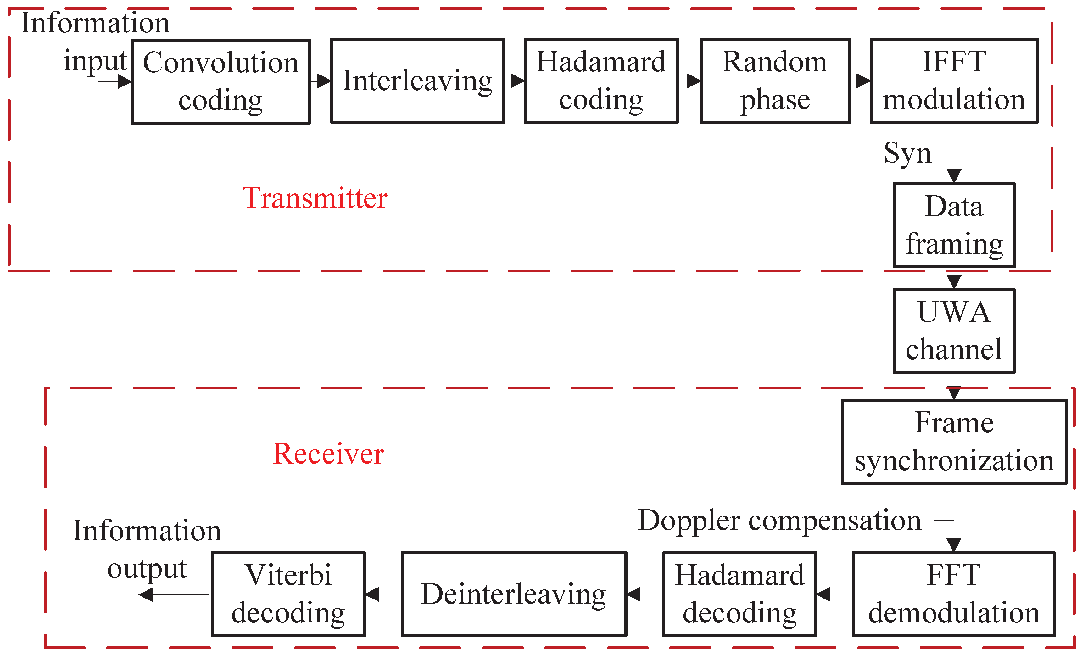
In this study, the overall system structure is shown in in Figure 1. One can see that at the transmitter, the information inputs were encoded by convolutional codes and then processed by interleaving and Hadamard coding. Random phase was used for reducing the peak to average ratio because we adopted inverse fast Fourier transform (IFFT) for MFSK modulation. A synchronization signal was then added, and the data stream was generated. The data were then transmitted through the underwater acoustic channel.

At the receiver, a matching filter was used for frame synchronization and then Doppler compensation via resampling. The data stream was then demodulated by FFT. Hadamard decoding and deinterleaving were used before the Viterbi decoding. The output value of deinterleaving provided a soft decision metric. Thus, it improved the performance of the joint decoding.

Considering that underwater acoustic communications are susceptible to systematic and random noise, we used forward error correction (FEC) for detecting and correcting a limited number of errors in the transmitted data without retransmission. Error correcting codes for FEC can be broadly categorized into two types, namely, block codes and convolution codes. The main differences between these codes are listed in

Table 1. The main differences between linear block codes and convolutional codes.

Linear Block Codes	Convolutional Codes
In linear block codes, information bits are immediately followed by the parity bits.	In convolutional codes, information bits are not followed by parity bits; instead, they are spread along the sequence.
Encoding of the current state is independent of the previous state; thus, it does not have any memory element. It depends only upon the present message bit.	Encoding of the current state depends on the previous state and past elements; thus, it has a memory element for storing previous state information.
The hardware component of block codes is complex, and the encoding process is a bit difficult.	The hardware component of convolutional codes is simpler, and the encoding process is easy.

.

The types of linear block codes are the Hamming codes, Walsh–Hadamard codes, cyclic codes, low-density parity-check (LDPC) codes, and the Reed–Solomon codes. The types of convolutional codes are the turbo codes and Trellis codes. Although the turbo code and LDPC code have good performance, the use of the turbo code or LDPC code is at the cost of implementation complexity. Turbo codes can obtain a higher coding gain only when the interleaving length is longer and the number of iterations is more. LDPC codes can obtain a higher coding gain only when the code length is longer. The long time delay affects the application of this kind of long code in underwater acoustic communications. Thus, concatenated coding is often used in this case. Considering that frequency diversity technology can effectively resist the frequency-selective fading of underwater acoustic channels, and the orthogonality of the Hadamard matrix facilitates distinguishing different codewords, we adopted the Hadamard code as an internal code and the convolutional code as an outer code. The details of the concatenated coding are as follows.

3.1. Hadamard Encoding and Decoding

The Hadamard matrix has excellent characteristics in that arbitrary codewords are orthogonal to each other. We adopted the Hadamard matrix to construct Hadamard codes. The Hadamard matrix ${\mathbf{H}}_n$ consists of $\{+1,-1\}$, with a size of $n\times n$. It has the property of

$$\begin{array}{c}\hfill {\mathbf{H}}_n{\mathbf{H}}_n^T=n\mathbf{I},\end{array}$$

(3)

where $\mathbf{I}$ is an identity matrix with size of $n\times n$. There are $n/2$ different elements between any two rows of the Hadamard matrix. It has a row of elements that are all 1 or all $-1$. We selected the other $2(n-1)$ rows of Hadamard and its complement matrices to construct the Hadamard codes. We selected $2^k$ rows from $2(n-1)$ rows to generate Hadamard codes $H(n,k)$, i.e., k bits of information were encoded into n bits by $H(n,k)$.

We adopted soft decision decoding for the Hadamard code. First, the square value of the signal amplitude of each subchannel was recorded with floating-point numbers. Then, the soft decision value was calculated, and the maximum soft decision value was selected as the final decoding result. We assumed that the fading signal and additive Gaussian white noise of each carrier frequency were independent, and the following soft decision was obtained.

$$\begin{array}{c}\hfill M_i=\sum _{j=1}^n{h}_{i,j}{\left|y_j\right|}^2,i=1,\cdots ,2^k,\end{array}$$

(4)

where $M_i$ is the soft decision value of the i-th Hadamard code, $h_{i,j}$ is the j-th bit of the i-th Hadamard code, and $|y_j{|}^2$ is the square value of the j-th carrier signal amplitude. In the joint decoding process, we adopted the maximum soft decision value $M_i$ as the branch metric in the Viterbi decoding process. In this study, we set $H(n_{\mathbf{H}}=20,k_{\mathbf{H}}=5)$. 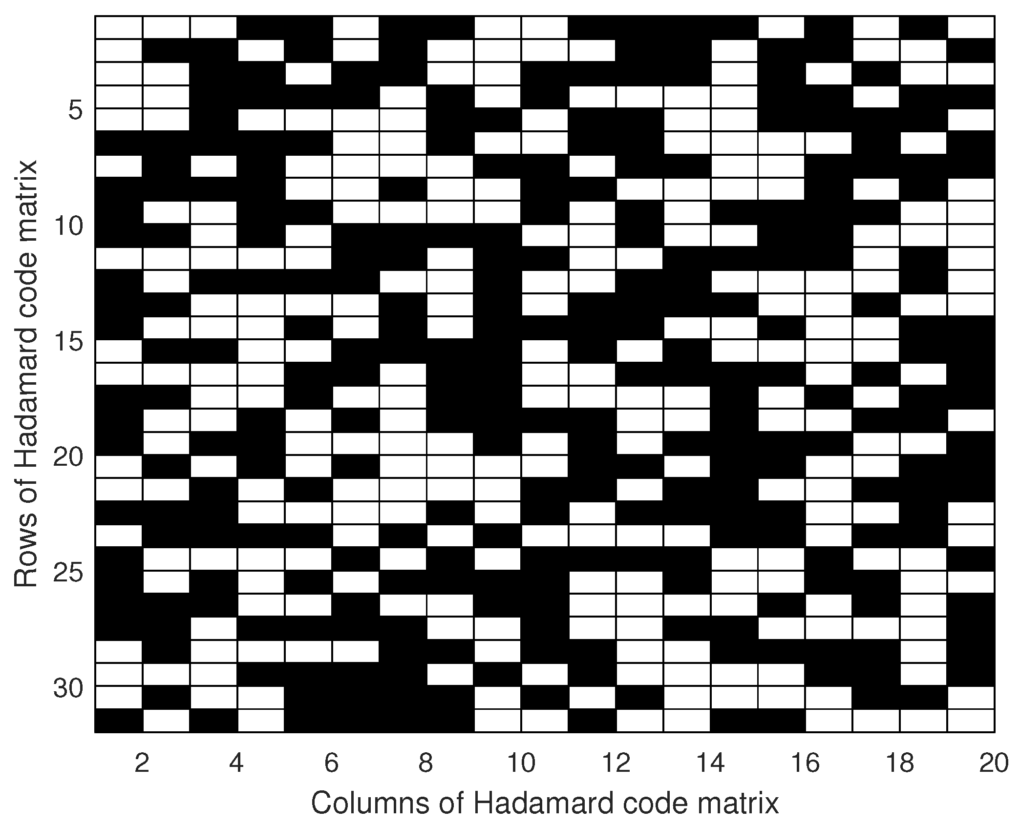The $\{+1,0\}$ element distribution of the Hadamard code matrix ${\mathbf{H}}_{(20,5)}$ is shown in Figure 2, where a black square represents 1, while a white square represents 0. The number of zeros and ones in each row was the same.

3.2. Convolution Encoding and Viterbi Decoding

The convolutional code $C(n,k,L)$ is a type of error-correcting code that generates parity symbols via the sliding application, where n, k, and L denote the output bits, input bits, and constraint length, respectively. The constraint length specifies the delay for the input bit streams to the encoder. The sliding nature of the convolutional codes facilitates trellis decoding using a time-invariant trellis, whose nodes are ordered into horizontal slices (time) with each node at each time connected to at least one node. Time-invariant trellis decoding allows maximum-likelihood soft-decision decoding with reasonable complexity. Then, the number of states of $C(n,k,L)$ is $N_{st}=2^{k(L-1)}$. In this study, we adopted $C(n_c=10,k_c=5,L_c=2)$. 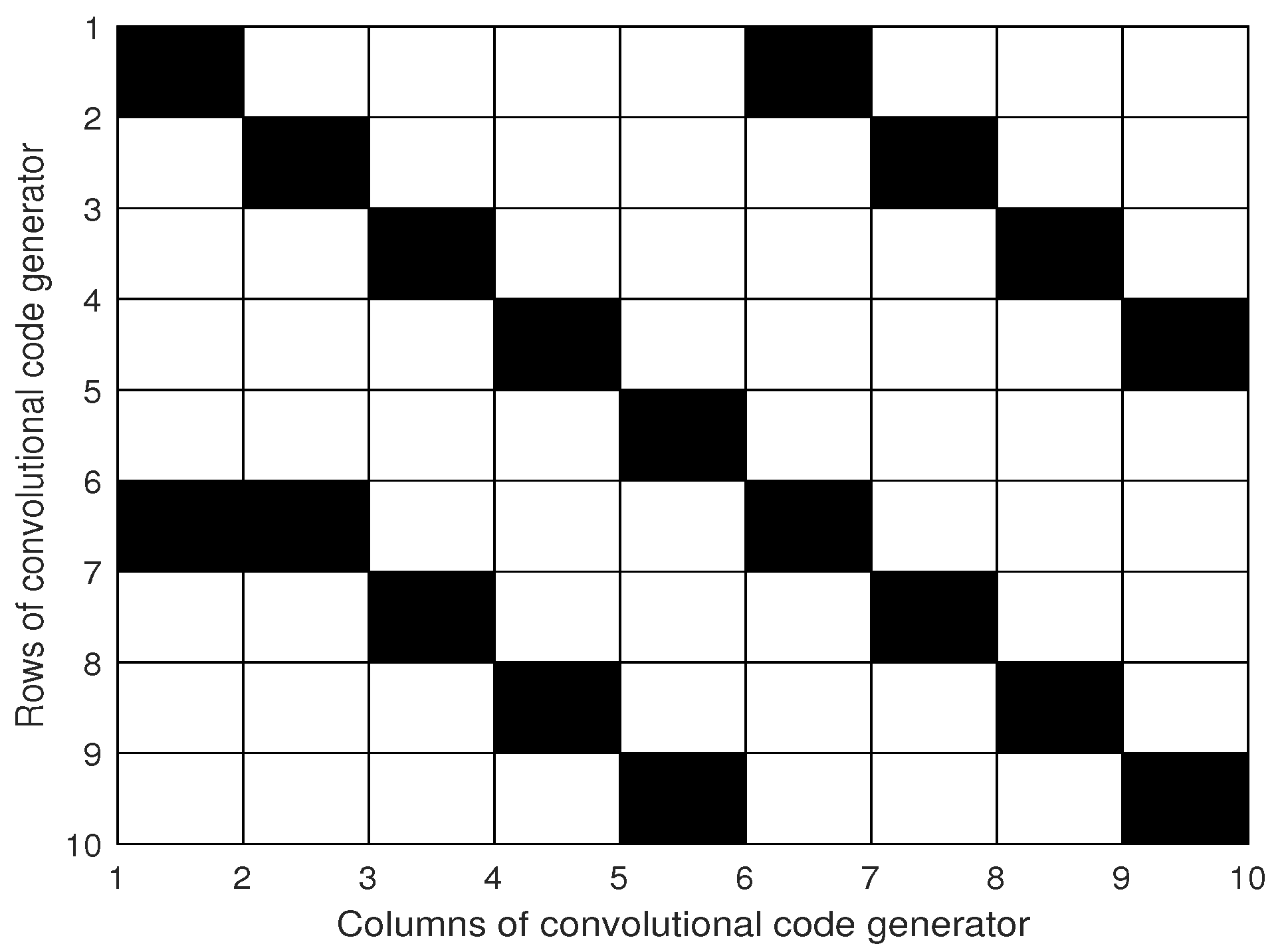The $\{+1,0\}$ distribution of the convolutional code generator is shown in Figure 3.

For convolution encoding, if n, k, L, and the generator are given, then the next state matrix (or named state transition matrix) ${\mathbf{S}}_c$, and the output matrix ${\mathbf{O}}_c$ can be computed. We adopted decimal representation for ${\mathbf{S}}_c$ and ${\mathbf{O}}_c$ in this study. The above parameters and matrices were used for the following encoding and decoding process.

The encoding steps of the convolution were as follows: We initialized the current state as $S^{t_n=0}=0$, where $t_n=0$ denoted the iteration time. We assumed the binary information bits $\mathbf{b}=\left\{b_i\right\},i=1,\cdots ,k$ were given. Then, we flipped it and transferred it to decimal digits d. The decimal output of the convolution encoder was

$$\begin{array}{c}\hfill d_o={\mathbf{O}}_c(S+1,d+1).\end{array}$$

(5)

The expression of $(S+1,d+1)$ was adopted as MATLAB code, because the row and column of a matrix cannot be indexed by 0 in that case. On the other hand, the next state was updated as

$$\begin{array}{c}\hfill S^{t_n+1}={\mathbf{S}}_c(S+1,d+1).\end{array}$$

(6)

The Viterbi algorithm has found universal application in decoding convolutional codes, and it is a dynamic programming algorithm for obtaining the maximum a posteriori probability estimate of the most likely sequence of hidden states. We used it as the joint decoding framework.

3.3. Concatenated Encoding and Signal Composition

After being processed by the convolution encoder, the length of the bit stream ${\mathbf{b}}_{in}=[b_i,{\mathbf{0}}_k]$ was double that of the previous one, where ${\mathbf{0}}_k$ was an all zero vector with a length of k. ${\mathbf{0}}_k$ ensured that the subsequent decoding returned to the 0 state. We denote the symbol ${\mathbf{b}}_{co}$ after the convolution encoder as

$$\begin{array}{c}\hfill {\mathbf{b}}_{co}=C_{(10,5,2)}\left({\mathbf{b}}_{in}\right).\end{array}$$

(7)

The encoded symbol ${\mathbf{b}}_{co}$ was interleaved by an interleaver, which was used to convert the convolutional codes from burst error correctors to random error correctors. The result was denoted by ${\mathbf{b}}_{cintl}$. We selected k elements from ${\mathbf{b}}_{cintl}$ as the row indexes of the Hadamard matrix and obtained the encoding process as:

$$\begin{array}{c}\hfill {\mathbf{H}}_{out}={\mathbf{H}}_{(20,5)}{({\mathbf{b}}_{cintl}+1,:)}^T.\end{array}$$

(8)

The matrix ${\mathbf{H}}_{out}$ was converted into a column vector via $\mathbf{h}=\mathrm{vec}\left({\mathbf{H}}_{out}\right)$.

After convolution encoding, interleaving, and Hadamard encoding, the information was modulated via MFSK. In order to maximize the frequency efficiency, we adopted the IFFT to allocate subcarriers. To reduce the peak-to-average ratio, we added the random phase $\varphi$ into the signal, as

$$\begin{array}{c}\hfill {\mathbf{h}}_{\varphi }=\mathbf{h}exp\left(j\varphi \right).\end{array}$$

(9)

Then, the MFSK signal was

$$\begin{array}{c}\hfill {\mathbf{x}}_{\mathrm{MFSK}}=\sqrt{N_{\mathrm{ft}}}\mathrm{IFFT}\left({\mathbf{h}}_{\varphi }\right),\end{array}$$

(10)

where $N_{\mathrm{ft}}$ is the number of the IFFT points.

The acoustic wave signals ${\mathbf{x}}_{\mathrm{MFSK}}$ were then transmitted through water. The multipath and Doppler of the UAC were the important factors when we designed the transmitted signal. Thus, the hyperbolic frequency modulation (HFM) signal was used as the head signal ${\mathbf{x}}_{\mathrm{HFM}}$ for synchronization and Doppler compensation. The HFM signal was

$$\begin{array}{c}\hfill {\mathbf{x}}_{\mathrm{HFM}}=Acos\left(2\pi klog(1-\frac{t}{t_0})\right),-\frac{T_s}{2}<t<\frac{T_s}{2},\end{array}$$

(11)

where

$$k=\frac{T_s{f}_2{f}_1}{f_2-f_1},t_0=\frac{T_s(f_2+f_1)}{2(f_2-f_1)},$$

$T_s$ denotes the time length of the HFM signal, and $f_2,f_1$ denote the max and min frequency of HFM signal, respectively.

3.4. Frame Synchronization and Doppler Compensation

The receiver has no information of the specific position of the frame synchronization signal. Therefore, the frame synchronization detection was designed by the maximum value of the correlation computation. The correlation peak was searched to determine the position of the frame synchronization signal in the received signal. The frame synchronization signal detection steps were as follows.

First, we set the number of points for FFT transform

$$\begin{array}{c}\hfill N_{\mathrm{fft}}=2^{\lceil {log}_2\left(2L_{\mathrm{HFM}}\right)\rceil },\end{array}$$

(12)

where $\lceil ·\rceil$ denotes the round up value, and $L_{\mathrm{HFM}}$ denotes the length of the HFM signal, e.g., if $L_{\mathrm{HFM}}=100$, then $N_{\mathrm{fft}}=256$.

Second, in order to generate the frequency domain representation of the HFM signal with $N_{\mathrm{fft}}$ points, we reversed the original HFM and added 0, as

$$\begin{array}{c}\hfill {\mathbf{s}}_{\mathrm{HFM}}\left(n\right)=\left\{\begin{array}{cc}{\mathbf{x}}_{\mathrm{HFM}}(L_{\mathrm{HFM}}-1-n)\hfill & (0\le n\le L_{\mathrm{HFM}}-1)\\ 0\hfill & (L_{\mathrm{HFM}}\le n\le N_{\mathrm{fft}}-1),\end{array}\right.\end{array}$$

(13)

where ${\mathbf{s}}_{\mathrm{HFM}}(-n)$ denotes the reverse signal ${\mathbf{x}}_{\mathrm{HFM}}\left(n\right)$. Then, we obtained the frequency domain representation

$$\begin{array}{c}\hfill {\mathbf{S}}_{\mathrm{HFM}}\left(k\right)=\sum _{n=0}^{N_{\mathrm{fft}}-1}{\displaystyle \frac{{\mathbf{s}}_{\mathrm{HFM}}\left(n\right)}{\left|\right|{\mathbf{s}}_{\mathrm{HFM}}\left(n\right)\left|\right|}}exp(-j2\pi nk/N_{\mathrm{fft}}).\end{array}$$

(14)

Third, we adopted the segmental interception of the received signal $\mathbf{y}$ (with a length of $L_{\mathbf{y}}$) to build the received signal for the search, denoted by ${\mathbf{y}}_r=[{\mathbf{y}}_2,{\mathbf{y}}_1]$, where ${\mathbf{y}}_1=\mathbf{y}(i:i+L_{\mathrm{diff}}-1),$$L_{\mathrm{diff}}=N_{\mathrm{fft}}-L_{\mathrm{HFM}},{\mathbf{y}}_2={\mathbf{y}}_1(\mathrm{end}-L_{\mathrm{HFM}}+1:\mathrm{end})$. The forward step of the selected data location point i was $L_{\mathrm{diff}}$. Then, the frequency domain representation of ${\mathbf{y}}_r$ is

$$\begin{array}{c}\hfill {\mathbf{Y}}_{\mathrm{r}}\left(k\right)=\sum _{n=0}^{N_{\mathrm{fft}}-1}{\displaystyle \frac{{\mathbf{y}}_{\mathrm{r}}\left(n\right)}{\left|\right|{\mathbf{y}}_{\mathrm{r}}\left(n\right)\left|\right|}}exp(-j2\pi nk/N_{\mathrm{fft}}).\end{array}$$

(15)

In fact, the result of correlation $\mathbf{z}\left(n\right)$ can be regarded as the inverse Fourier transform of the product of ${\mathbf{Y}}_{\mathrm{r}}\left(k\right)$ and ${\mathbf{S}}_{\mathrm{HFM}}\left(k\right)$. Thus,

$$\begin{array}{c}\hfill \mathbf{z}\left(n\right)=\sum _{n=0}^{N_{\mathrm{fft}}-1}{\mathbf{Y}}_{\mathrm{r}}\left(k\right){\mathbf{S}}_{\mathrm{HFM}}\left(k\right)exp(j2\pi nk/N_{\mathrm{fft}}).\end{array}$$

(16)

One can select the maximum value $A_p$ and its location $P_m$ of $\mathbf{z}\left(n\right)$. Then, the start time point is $T_s=P_m-L_{\mathrm{HFM}}$. If $T_s<0$ or $A_p<Th$, where $Th$ is a threshold for weak signal detection, then the data location point moves forward as $i=i+L_{\mathrm{diff}}$.

After frame synchronization, the components of the receiver also included the following parts: Doppler estimation and compensation, MFSK demodulation, and joint decoding. We assumed the packet lengths of the received and transmitted signal were $T_{\mathrm{rp}},T_{\mathrm{tp}}$; then, the Doppler was estimated as

$$\begin{array}{c}\hfill \mathsf{\Delta }={\displaystyle \frac{T_{\mathrm{rp}}}{T_{\mathrm{tp}}}}-1.\end{array}$$

(17)

It is worth noting that $T_{\mathrm{rp}}$ is critical to the estimation accuracy of Doppler. Two locations of an HFM signal can be found in the received signal by finding the maximum value of its correlation operation between the HFM signal and the received signal.

Thus, the resampling rate $f_{\mathrm{rs}}$ is

$$\begin{array}{c}\hfill f_{\mathrm{rs}}=(1+\mathsf{\Delta })f_s,\end{array}$$

(18)

where $f_s$ is the original sampling rate.

3.5. Demodulation and Joint Decoding

Then, the signal was demodulated by the MFSK, shown as

$$\begin{array}{c}\hfill {\mathbf{y}}_{\mathrm{MFSK}}={\displaystyle \frac{1}{\sqrt{N_{\mathrm{ft}}}}}\mathrm{FFT}\left({\mathbf{x}}_{\mathrm{MFSK}}\right).\end{array}$$

(19)

The demodulated MFSK signal was chosen by its subcarrier index $I_{\mathrm{subcarrier}}$ and then processed by deinterleaving, resulting in

$$\begin{array}{c}\hfill {\mathbf{y}}_{\mathrm{deintl}}=\mathrm{Deintl}\left[\right|{\mathbf{y}}_{\mathrm{MFSK}}\left(I_{\mathrm{subcarrier}}\right){|}^2].\end{array}$$

(20)

The result ${\mathbf{y}}_{\mathrm{deintl}}$, which was the input of the joint decoder, was reshaped as a matrix $\mathbf{Y}$ with the size of $L_g\times T_f$, where $L_g=n_{\mathbf{H}}{n}_c/k_c$, $T_f$ was the time length of $\mathbf{Y}$ per frame.

The pseudo codes of the joint decoding algorithm are displayed in a MATLAB-like way in Algorithm 1. The bold uppercase letter denotes a matrix, while the bold lowercase one denotes a vector. ${\mathbf{0}}_{N_{st}\times (T_f+1)}$ denotes the elements in a matrix of size $N_{st}\times (T_f+1)$ are all 0, where $N_{st}$ denotes the number of states, and $T_f$ denotes the data length of a frame. de2bi converts decimal numbers to their binary representations. ${\mathbf{O}}_c,{\mathbf{S}}_c$ denote the output matrix and the state transition matrix, respectively. $\mathbf{H}$ denotes the Hadamard matrix.

Algorithm 1 The pseudo codes of the joint decoding algorithm

Input: received signal $\mathbf{Y}$, $\mathbf{H},{\mathbf{O}}_c,{\mathbf{S}}_c$ Output: decoding bits $\widehat{\mathbf{x}}$  Initialization: branch metric matrix ${\mathbf{M}}_b={\mathbf{0}}_{N_{st}\times (T_f+1)}$;  final state matrix ${\mathbf{S}}_f={\mathbf{0}}_{N_{st}\times (T_f+1)}$;  previous state vector ${\mathbf{s}}_p={\mathbf{0}}_{N_{st}\times 1}$;  next state vector ${\mathbf{s}}_n={\mathbf{0}}_{N_{st}\times 1}$.  while $t\le T_f$ do     $\mathrm{Initialization}:\mathrm{path}\mathrm{metric}{\mathbf{m}}_p^{t=0}=-\infty$,     $\mathrm{new}\mathrm{metric}{\mathbf{m}}_n^{t=0}=-\infty$, all with size of $N_{st}\times 1$;     while $i\le N_{st}$ do       ${\mathbf{b}}_o=\mathrm{de}2\mathrm{bi}{\left[{\mathbf{O}}_c(i,:)\right]}^T$; convert decimal to binary.       branch metric: ${\mathbf{m}}_b^t=DH(\mathbf{Y}(:,t),{\mathbf{b}}_o,\mathbf{H},n_c,k_c)$;       ${\mathbf{m}}_n({\mathbf{S}}_c{(i,:)}^T+1)={\mathbf{M}}_b(i,t)+{\mathbf{m}}_b^t$;       $[{\mathbf{m}}_p^{t+1},I_{{\mathbf{m}}_p^{t+1}}]=max[{\mathbf{m}}_p^t,{\mathbf{m}}_n]$;       ${\mathbf{s}}_p({\mathbf{S}}_c{(i,:)}^T+1)=i-1$;       ${\mathbf{s}}_n=[{\mathbf{s}}_n,{\mathbf{s}}_p](I_{{\mathbf{m}}_p^{t+1}})$;       $i=i+1$;     end while     ${\mathbf{S}}_f(:,t+1)={\mathbf{s}}_n$;     ${\mathbf{M}}_b(:,t+1)={\mathbf{m}}_p$;     $t=t+1$;  end while  Initialization: signal estimation $\widehat{\mathbf{x}}={\mathbf{0}}_{N_{st}\times T_f},i=0$;  while $t\le T_f$ do     current state: ${\mathbf{s}}_c={\mathbf{S}}_f(i+1,T_f-t+2)$;     $\widehat{\mathbf{x}}(:,T_f-t+1)=\mathrm{flip}\left\{\mathrm{de}2\mathrm{bi}[{\mathbf{S}}_c({\mathbf{s}}_c+1,:)==i,k_c]\right\}$;     $i={\mathbf{s}}_c$;  end while  Obtain the signal estimation $\widehat{\mathbf{x}}$.

The pseudo codes of the distance of the Hadamard (branch metric) are displayed in Algorithm 2, where $n_c$ and $k_c$ denote the output length as $n_c$, when the data length $k_c$ is encoded by the Hadamard matrix $\mathbf{H}$. The column number of $\mathbf{H}$ is denoted by $n_{\mathbf{H}}$

Algorithm 2 The pseudo codes of the distance of the Hadamard algorithm, i.e., ${\mathbf{m}}_b^t=DH(\mathbf{Y}(:,t),$${\mathbf{b}}_o,\mathbf{H},n_c,k_c)$

Input: receive signal $\mathbf{Y},\mathbf{H}$, ${\mathbf{b}}_o,n_c,k_c$ Output: branch metric ${\mathbf{m}}_b^t$  convert bits ${\mathbf{b}}_o$ to $k_{\mathbf{H}}$-ary symbols ${\mathbf{s}}_o$;  Hadamard encoding process ${\mathbf{H}}_{out}=\mathbf{H}{({\mathbf{s}}_o+1,:)}^T$;  reshape ${\mathbf{H}}_{out}$ with size of $[n_{\mathbf{H}}{n}_c/k_c]\times N_{st}$;  Obtain the branch metric ${\mathbf{m}}_b^t={\mathbf{Y}}^T{\mathbf{H}}_{out}$.

The parameters of the Hadamard code and the convolutional code are shown in

Table 2. The parameter settings of the convolutional code and the Hadamard code.

The Parameter Settings	Value
Convolutional code output bits $n_c$	10
Convolutional code input bits $k_c$	5
Generate Matrix size	$5\times 10$
Output Matrix size	$32\times 32$
Next States Matrix size	$32\times 32$
Hadamard code output bits $n_{\mathbf{H}}$	20
Hadamard code input bits $k_{\mathbf{H}}$	5
Hadamard Matrix size	$32\times 20$
Nfft	4096

.

3.6. Data Frame Format

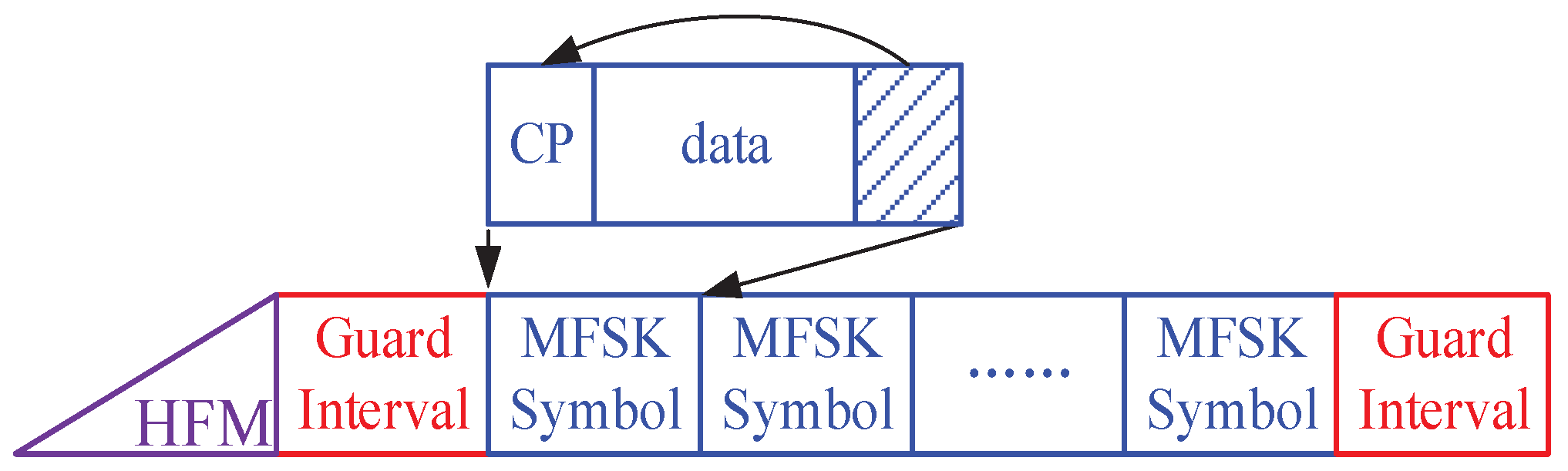
In this study, we adopted the data frame format shown in Figure 4. HFM was used as synchronization. A guard interval (GI) was set between the synchronization signal and symbols to reduce the interference with the data segment when the receiver correlated the synchronization signal. Each MFSK symbol was composed of a cyclic prefix (CP) and information data symbols. The CP was added to resist inter symbol interference and inter-subcarrier interference caused by multipath channels. The length of the CP should be greater than the maximum length of the multipath delay, to ensure that the delay spread of the previous symbol will fall within the CP and not affect the demodulation of the current symbol.

We assumed that each frame contained 20 MFSK symbols, each MFSK symbol contained eight Hadamard symbols, and each Hadamard symbol contained 20 bits but only 5 bits of information. Thus, each frame contained $20\times 8\times 5=800$ bits of information. However, the convolution rate was 1/2 with the $k_c$ redundant bit. Thus, the information bits were $400-k_c$.

4. Simulations

In order to simulate the actual sea trial environment, we set the parameters as shown in

Table 3. The parameter settings in the simulations.

The Parameter Settings	Value
Source depth	2 m
Receiver depth	2 m
Transmission distance	1 km
Central frequency	21 kHz
Doppler shift	20 Hz
Sampling frequency	96 kHz
Band width	6 kHz
Time of HFM	20 ms
Time of CP	40 ms
Time of GI	100 ms
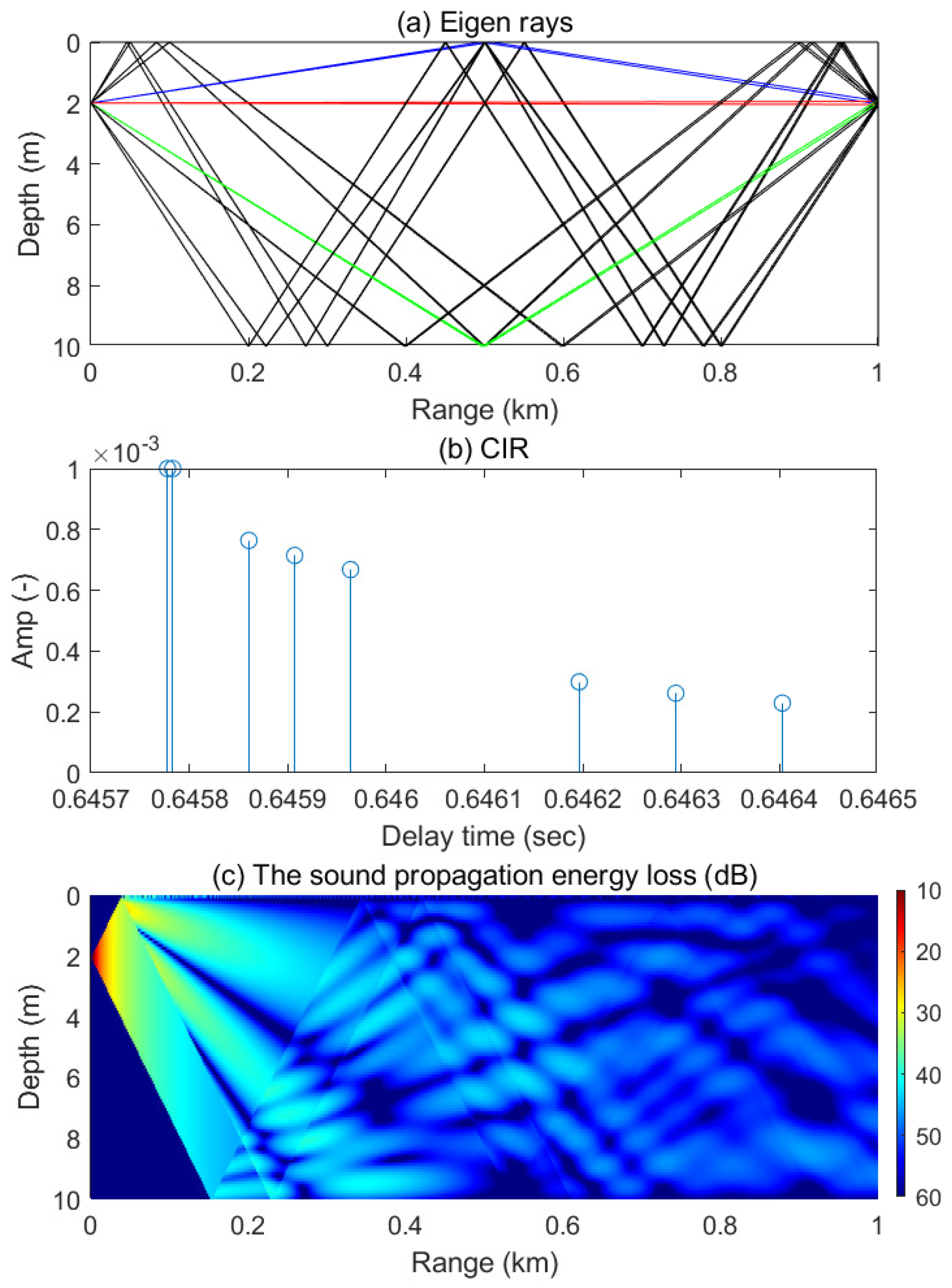
Nfft	4096

. Considering the water depth was low, we simulated the channel environment as an iso-velocity channel. We used BELLHOP to generate the Eigen sound ray as shown in Figure 5a, its CIR as shown in Figure 5b, and its sound propagation energy loss diagram as shown in Figure 5c. The CIR was used to simulate the actual channel and obtain the filtered signal as the received signal. Additive white Gaussian noise (AWGN) was used for the channel coding performance tests.

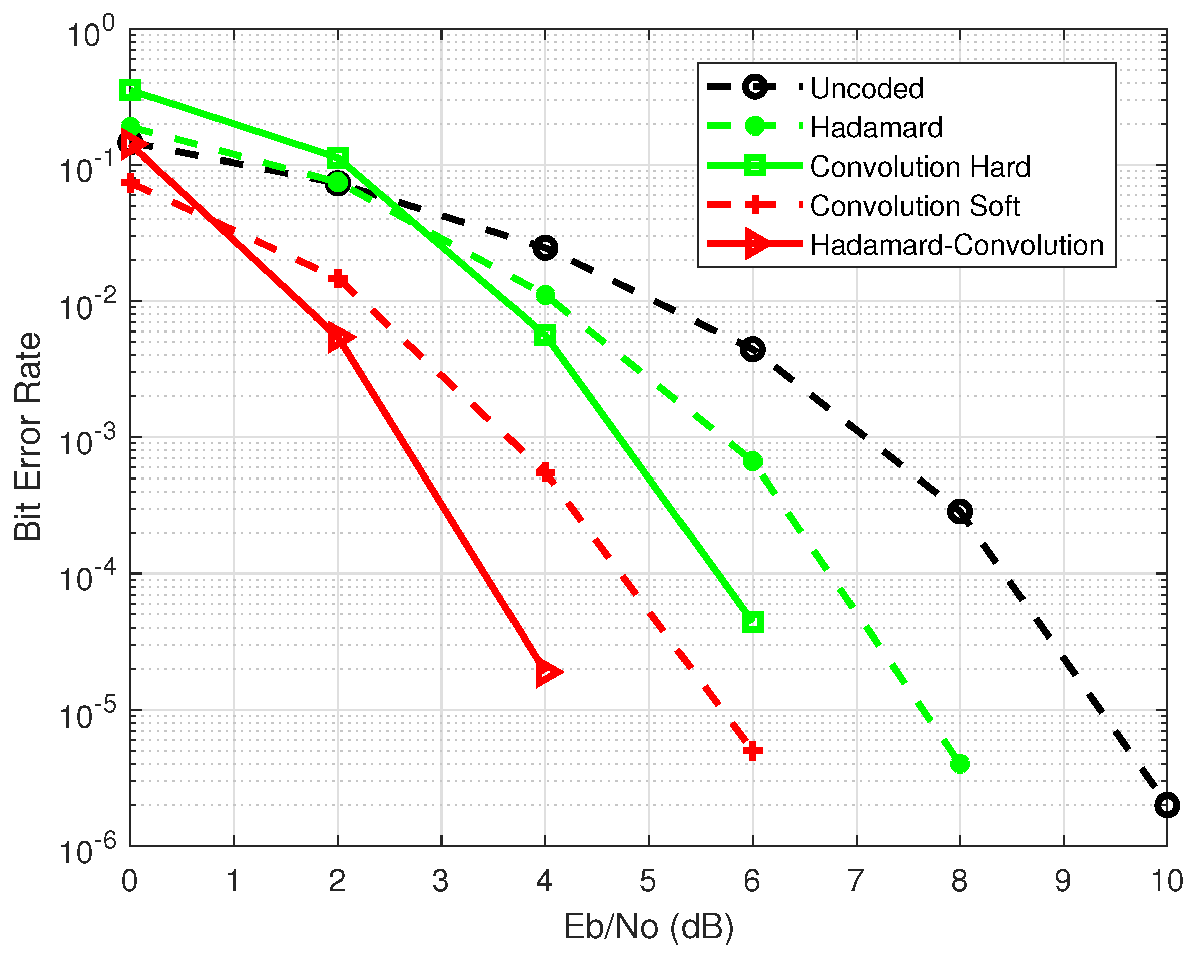
In order to test the concatenated coding and its decoding bit error ratio (BER) performance, we used convolution codes with hard and soft decoding and Hadamard decoding for comparisons. The transmitted signal was passed through the simulated channel. The constraint length was set as seven, while the code generator was expressed in octal as [171, 133]. The traceback depth was set as 32. The coding rate for the convolution code was 1/2. We adopted quadrature amplitude modulation (QAM) (M = 4) and demodulation. For soft Viterbi decoding in the convolution code, the output values of QAM were calculated using the approximate log-likelihood algorithm.

The results are shown in Figure 6, where Eb is the signal energy associated with each data bit, i.e., the signal squared amplitude divided by 2 times the user bit rate. No is the noise spectral density, i.e., the noise power in a 1 Hz bandwidth. One can see that the proposed concatenated coding had the lowest BER compared to the counterparts including the Hadamard and convolution codes with hard and soft decisions.

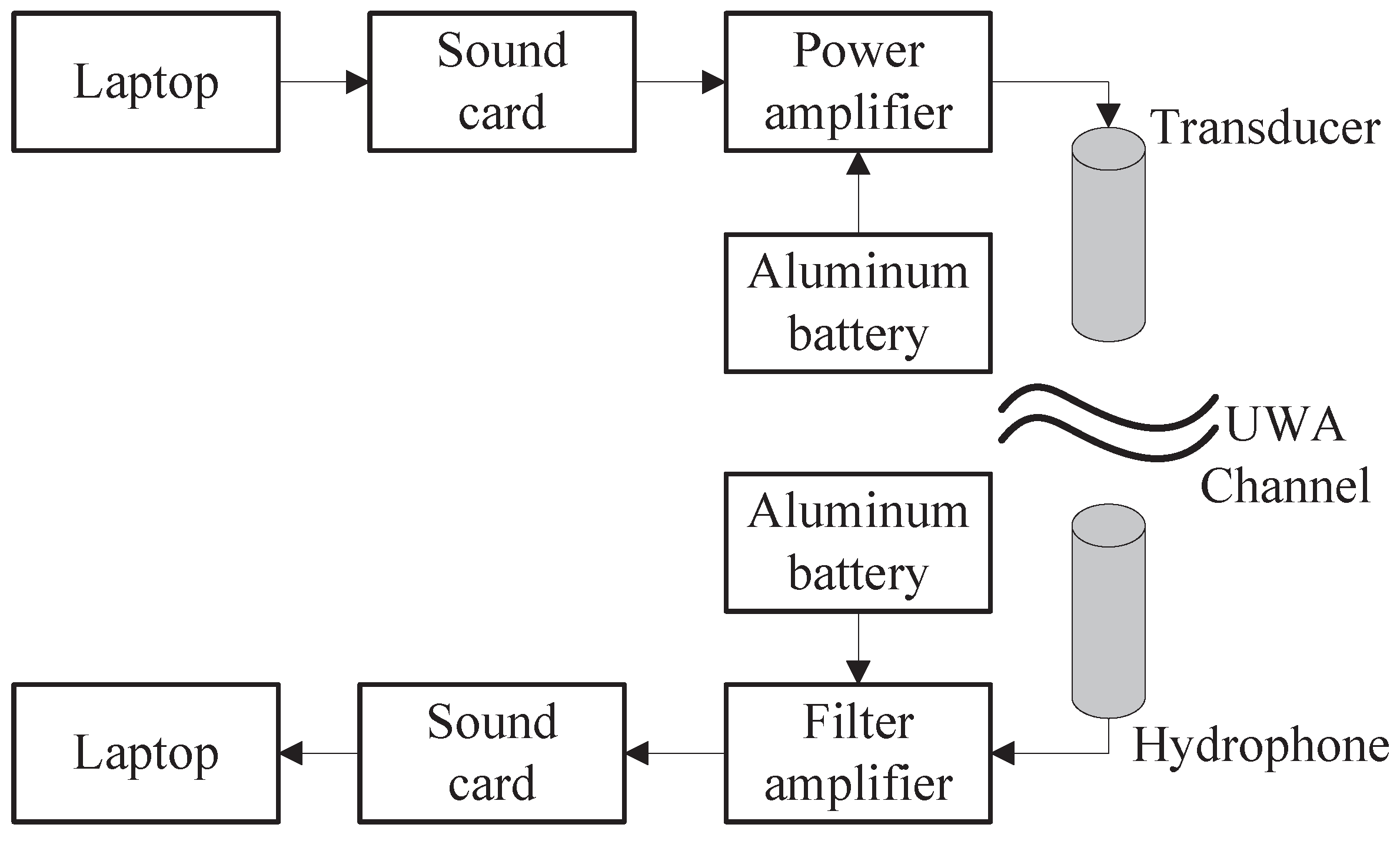
5. At-Sea Experiment

In this section, the at-sea experiment conducted to test the performance of the concatenated coding of MFSK underwater acoustic communications is described. The experiment location was Wuyuan Bay in Xiamen, China. The environmental parameters are shown in

Table 4. The environmental parameters.

The Parameters	Value
Source depth	2 m
Receiver depth	2 m
Transmission distance	1 km
Central frequency	21 kHz
Sampling frequency	96 kHz
Band width	6 kHz
Time of HFM	20 ms
Time of CP	40 ms
Time of GI	100 ms
Nfft	4096

. The overall system structure of the transmitter and receiver is shown in Figure 7. The center frequency of the filter circuit was 30 kHz, the bandwidth was 25 kHz, the passband gain was 15 dB, the maximum attenuation was −3 dB, the passband ripple was 0.02 dB, and the stopband attenuation was −20 dB.

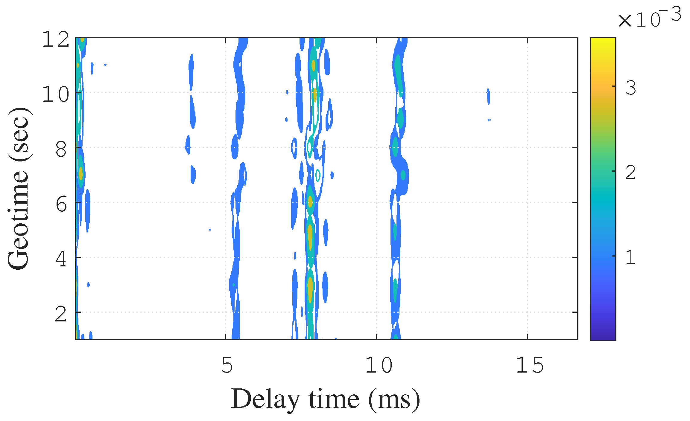
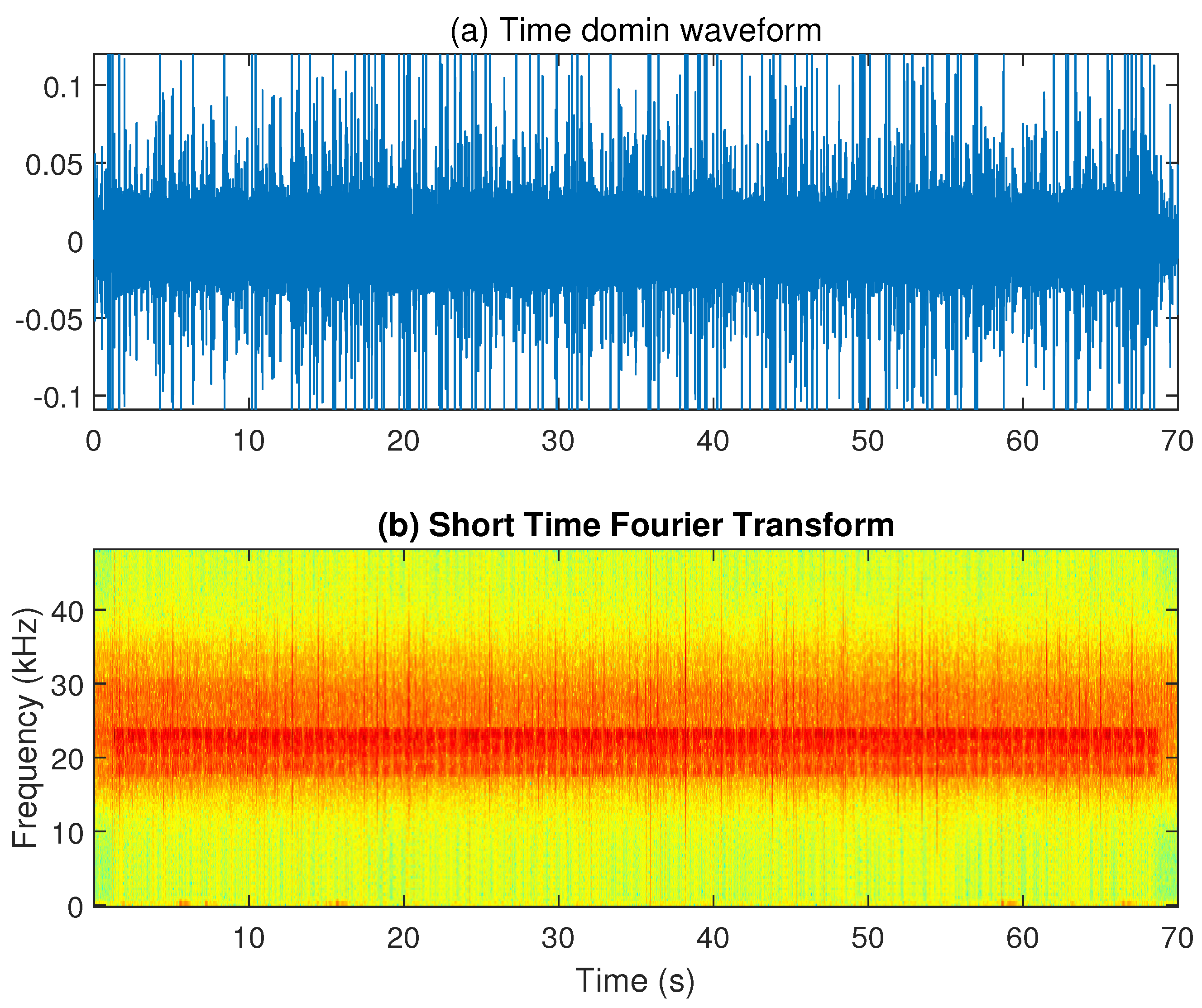
We obtained the channel impulse response (CIR) as shown in Figure 8 with the transmitted and received signal. It is obvious that the multipath structure varied. The variation in the CIR resulted in a 2 Hz Doppler spread.

Different from the traditional MFSK method, we took M = 240 in this study, because we took 12 rows from the Hadamard matrix, transposed them, and processed them by a vectorization operation. Considering $n_{\mathbf{H}}=20$, we know that the subcarrier number for the data was M = 240.

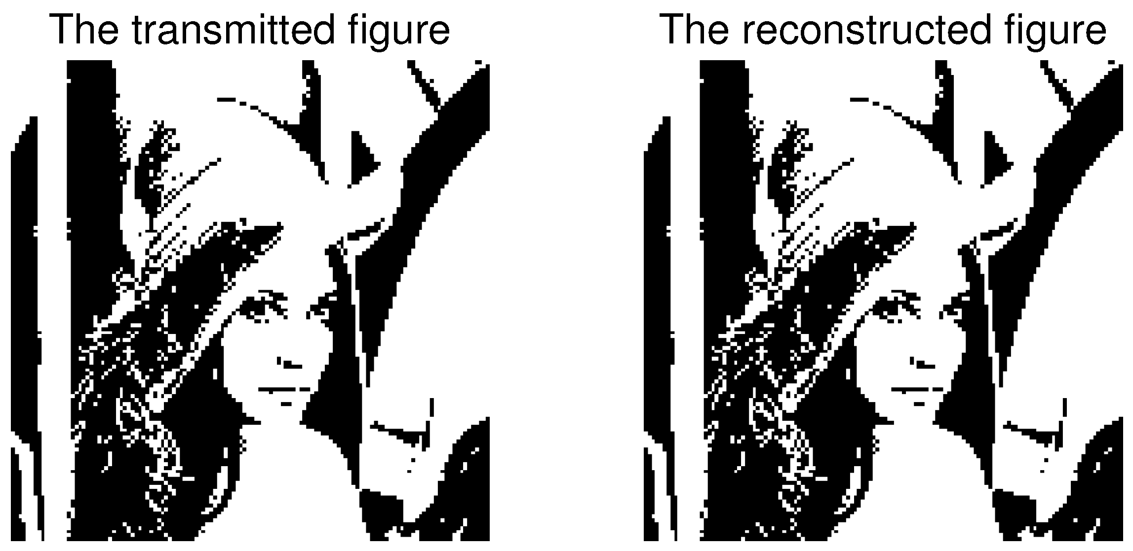
The transmitted information was a binary “Lena” graph, with the size of $128\times 128$. The received signal is shown in Figure 9; the received signal SNR was around 10 dB. The transmitted figure and the reconstructed one in the receiver are shown as Figure 10. The BER of the receiver was 0 in this case. Furthermore, when we added the AWGN to the received signal to test the robustness of the proposed communication framework to noise, the lowest SNR was 0 dB, and we retained the BER of 0.

6. Conclusions

This study adopted Hadamard–convolution concatenated coding and joint decoding, CP, Doppler compensation, interleaving, frame synchronization, etc., to form a robust underwater acoustic communication in a complete system way. Different from the traditional MFSK system, we designed a new MFSK with the concept of OFDM, i.e., M = 240. The channel-concatenated coding consisted of a Hadamard code and a convolutional code. Correspondingly, the iterative joint decoding used the Hadamard–Viterbi joint soft decoding framework. The soft decision mode was based on a newly designed branch metric, which was incorporated into the Hadamard structure. Comparisons among several channel coding methods were conducted to confirm the superiority of the joint channel-concatenated coding. Simulations and at-sea experiments were conducted to confirm the effectiveness of the proposed communication framework.