Review

Detection of Surface Water and Floods with Multispectral Satellites

1
Dipartimento di Scienze del Suolo, della Pianta e degli Alimenti, Università degli Studi di Bari Aldo Moro, Via G. Amendola 165/a, 70126 Bari, Italy
2
Dipartimento di Ingegneria Civile, Ambientale, del Territorio, Edile e di Chimica, Politecnico di Bari, Via Edoardo Orabona 4, 70125 Bari, Italy
3
Dipartimento di Ingegneria Civile, Edile e Ambientale, Università degli Studi di Napoli Federico II, Via Claudio 21, 80125 Napoli, Italy
*
Author to whom correspondence should be addressed.
Remote Sens. 2022, 14(23), 6005; https://doi.org/10.3390/rs14236005
Submission received: 4 October 2022 / Revised: 27 October 2022 / Accepted: 24 November 2022 / Published: 27 November 2022

Abstract

:
The use of multispectral satellite imagery for water monitoring is a fast and cost-effective method that can benefit from the growing availability of medium–high-resolution and free remote sensing data. Since the 1970s, multispectral satellite imagery has been exploited by adopting different techniques and spectral indices. The high number of available sensors and their differences in spectral and spatial characteristics led to a proliferation of outcomes that depicts a nice picture of the potential and limitations of each. This paper provides a review of satellite remote sensing applications for water extent delineation and flood monitoring, highlighting trends in research studies that adopted freely available optical imagery. The performances of the most common spectral indices for water segmentation are qualitatively analyzed and assessed according to different land cover types to provide guidance for targeted applications in specific contexts. The comparison is carried out by collecting evidence obtained from several applications identifying the overall accuracy (OA) obtained with each specific configuration. In addition, common issues faced when dealing with optical imagery are discussed, together with opportunities offered by new-generation passive satellites.

1. Introduction

Remote sensing techniques play a crucial role in monitoring water bodies and assessing river dynamics, providing effective support to surface water management. Considering the growing availability of medium–high-resolution and free remote sensing data, both active and passive sensors onboard different satellites are being extensively used for water segmentation and flood mapping. Satellite data are, in fact, of particular interest when observations over wide areas are necessary, for example, to assist with large-scale flood phenomena [1]. Active and passive satellite sensors operate in the microwave segment of the electromagnetic spectrum, while passive satellites include both sensors operating in the microwave spectrum segment and in the portion from the visible to the thermal infrared (optical imagery). Although active microwave sensors provide their own source of illumination, thus being in operation day and night and under all weather conditions, the use of passive multispectral sensors is relatively straightforward [1], and observations are easily interpretable. The availability of several spectral bands with different wavelengths, in fact, makes it possible to derive valuable information from each band and surfaces’ spectral signatures, or through direct interpretation of true- and false-color composites. In addition, with simple math algebra, vegetation indices exploit the reflectance characteristics of different objects.
Multispectral images have been successfully used for water body and river monitoring, change detection, and water feature extraction [2,3,4,5]. In addition, when cloud cover does not represent a major issue, the application of optical remote sensing to maps of flooded areas [6,7,8] offers the possibility of quickly and reliably identifying hazardous areas and supporting the implementation of flood coping strategies and response activities. In this context, the use of Unmanned Aerial Systems (UASs) may also provide high-resolution data in the presence of clouds, given the low-altitude range of these systems that allow flying below the cloud layer to be achieved (e.g., [9,10]). Moreover, the advent of Global Navigation Satellite System (GNSS) and, in particular, the Cyclone GNSS (CYGNSS) constellation, has recently demonstrated the potential of passive microwave instruments to estimate flood inundation and map inland surface water [11,12,13,14,15,16]. In fact, CYGNSS benefits from the L-band microwave capabilities of penetrating cloud cover and low–medium vegetation density, thus avoiding scattering problems due to precipitation and clouds [17].
Multispectral satellite data have also been recently proven to be suitable for monitoring the long-term spatio-temporal dynamics of river planform morphology and vegetation coverage, as well as land use/land cover evolution [18,19,20,21]. Boothroyd et al. [18] used vegetation indices derived from multispectral images to assess changes in the wetted river planform morphology and vegetation coverage along Po River Basin (Italy) with a multi-temporal Landsat image analysis (from 1988–2018). Similarly, Henshaw et al. [19] used Landsat scenes to determine the spatio-temporal trends of vegetation extent and channel position of six different sites along Tagliamento River (Italy). The incorporation of morphological processes into the evaluation of flood hazard has been carried out over both long- [18,19] and short-term timescales [22] and has shown to be of relevance for flood risk management. In addition, the hydrodynamics characteristics of the flow during a flooding event can modify vegetation coverage and flow resistance through erosion and sediment deposition [23,24]. In this regard, the information that can be inferred from optical remote sensing data represents a unique opportunity for monitoring planform, vegetation, and land cover changes, improving and supporting flood hazard predictions and modelling.
Over the past few years, different methods for water segmentation and flooded area mapping using multispectral satellite images have been proposed in the literature. These are generally divided into single-band and multi-band approaches. While the former discriminates water features from other surfaces by thresholding a single band, usually the near infrared (NIR), which is highly absorbed by water, the latter uses a combination of two or more bands for deriving spectral indices. The multi-band method, also called water index method, is a promising approach for surface water mapping both in data-rich and data-poor catchments [25]. It performs better than the single-band method in detecting land surface water, since it exploits differences in the reflectivity of the selected bands [26].
Multispectral remote sensing-derived indices allow flooded areas and water bodies to be quickly and effectively recognized. However, this ability can be highly compromised by the presence of scattering noise, built-up areas, clouds, and shadows. In addition, spectral index performances can be different according to the geomorphological conformation of the territory, as well as the land cover conditions, i.e., crops, forests, artificial surfaces, or open water.
In this context, this paper aimed to gain insights into the state of the art of multispectral satellite remote sensing and approaches to water extent delineation and flood mapping. In detail, the review aimed to achieve the following:
(a)
Providing an overview of the current optical satellites used in flooded area and wetland inundation mapping, with a focus on some of the medium–high-spatial resolution sensors that offer free-of-charge data.
(b)
Highlighting the potential and limitations of the use of spectral indices for flood mapping and water segmentation, with particular attention to the land cover setting.
A systematic review to address the first objective was initially carried out. The analysis of the literature allowed us to identify the most frequently used sensors in flood detection studies, as well as the main approaches and advances. Then, to address the second objective, a further investigation of the literature was conducted to identify relevant studies that used spectral indices for water extent delineation and flooded area detection. Several authors compared the use of different water index methods for both surface water body extraction [5,27,28,29] and flood mapping [30,31,32]. Therefore, we summarized the main outcomes from the literature, identifying the most reliable indices to detect the presence of water (i.e., open water or flooded areas). In addition, a further analysis of the selected literature was conducted to classify the performances of the most used multispectral indices according to the land cover conditions, with the aim to provide guidance for targeted applications of flood mapping using multispectral remote sensing. The spectral indices considered included, among others, the Normalized Difference Vegetation Index (NDVI [33]), the Normalized Difference Water Index (NDWI [34]), and the Modified Normalized Difference Water Index (MNDWI [26]).
The manuscript is organized into five sections, including the introduction. Section 2 describes the main characteristics of the most common optical satellites that offer free-of-charge data to provide a summary of their characteristics and data accessibility. The methodology adopted to conduct the proposed systematic review in the context of flood detection and hazard mapping from selected optical remote sensors is also illustrated, and an analysis of the main trends emerging from this review is presented. Section 3 introduces the most used spectral indices for the extraction of surface water extent and describes the main characteristics of a performance assessment for image classification and the corresponding error metrics. In addition, the investigation of the performances of the selected indices, based on evidence from the literature, is presented, and the classification of the accuracy values, according to the land cover conditions, is proposed. In Section 4, the main outcomes are described; finally, in Section 5, the conclusions are drawn, and future research directions are discussed.

2. Multispectral Satellite Remote Sensing for Flooded Area and Wetland Inundation Mapping

Since the mid-1970s, several optical satellites have been monitoring the Earth’s surface. The Landsat program represents the oldest and longest-running satellite mission, operating since July 1972, when Landsat 1 was first launched. Over the years, new satellites equipped with different instruments were placed in orbit, and the most recent mission, represented by the Landsat 9 satellite, was recently launched in September 2021. Satellites still in operation are Landsat 7, Landsat 8, and the aforementioned Landsat 9. Optical sensors onboard these satellites capture images at different spectral (i.e., wavelengths and bandwidths) and spatial resolutions, with a common revisit time of 16 days.
The Moderate Resolution Imaging Spectroradiometer (MODIS) instrument operates on the Terra and Aqua satellites, respectively launched in December 1999 and May 2002, and captures images in 36 spectral bands. Despite its coarse spatial resolution (see Table 1), MODIS has a daily revisit time, which is one of the most important factors when data obtained during the flood event are needed for flood extent delineation [35].
Sentinel-2 is a constellation formed by two twin satellites, S-2A and S-2B, respectively launched in June 2015 and March 2017, that together ensure a revisit time of 5 days. A multispectral instrument (MSI) mounted on Sentinel-2 provides images in 12 spectral bands (see Table 1). Together with Landsat, Sentinel-2 constitutes the family of medium–high spatial resolution multispectral satellites.
The National Oceanic and Atmospheric Administration’s (NOAA) Advanced Very High-Resolution Radiometers (AVHRR) sensor has been equipped on polar orbiting weather satellites since 1978. Since then, different instruments onboard several satellites have been imaging the Earth. The last version, AVHRR/3, currently operating on NOAA-15, -18, and -19 satellites, acquires daily images in six spectral bands (from the visible to the infrared portions of the electromagnetic spectrum) with a spatial resolution of 1.1 km, making it possible to perform flood mapping at very large scales.
These are examples of passive remote sensing programs offering free-of-charge data. In this work, we reviewed the use of medium–high-spatial resolution imagery for flooded area and wetland inundation mapping. In addition, as reviewed by Zhao et al. [40], Sentinel, Landsat, and MODIS are the most significant Earth observation satellite missions, based on the remote sensing impact index (RSIF) built by the authors, that will likely still be on the front line for environmental monitoring. For these reasons, we focused on the Landsat, MODIS, and Sentinel-2 satellites in our review.
Table 1 illustrates the main spectral and spatial resolution characteristics of Landsat 4- and 5-Thematic Mapper (TM), Landsat 7-Enhanced Thematic Mapper Plus (ETM+), Landsat 8-Operational Land Imager (OLI) and Thermal Infrared Sensor (TIRS), Sentinel-2 MSI, and Terra–Aqua MODIS instruments, with a particular focus on spectral bands commonly used in surface water monitoring studies. In addition, references and links to the data portals from which it is possible to visualize and freely download multispectral images from these satellites are provided in the same table.

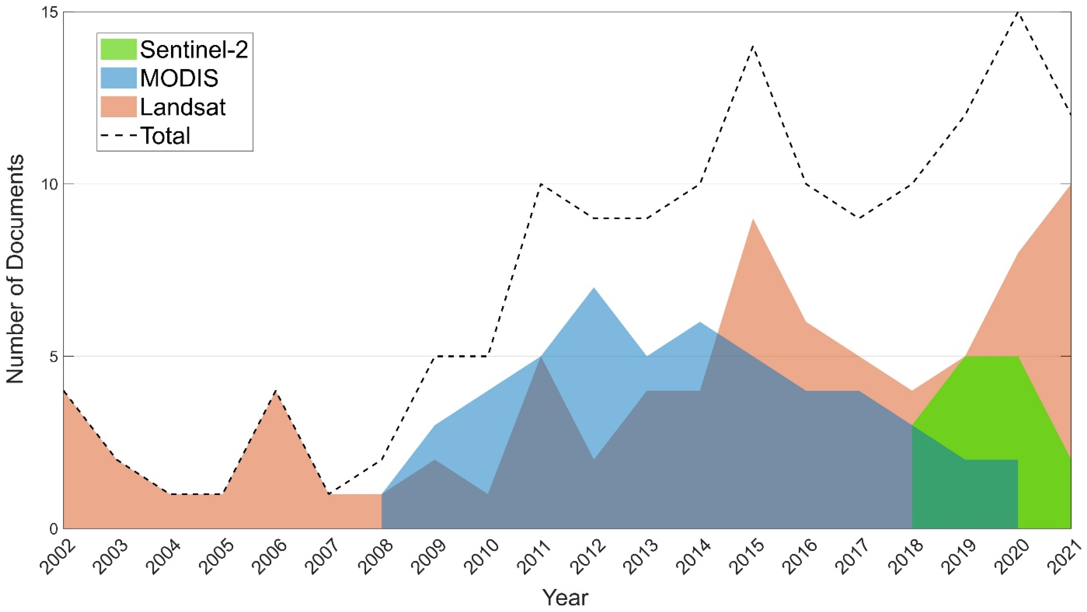
2.1. Trends in Using Multispectral Imagery for Flood Mapping

The international Scopus academic database was used to acquire the relevant literature in the field of flood mapping extracted from free-of-charge optical satellite data. The multispectral sensors considered for the review were the Landsat, Sentinel-2, and MODIS satellites. An initial exploration was carried out using a list of keywords for each satellite. An example of search instructions for the Landsat program is the following: (flood AND mapping AND Landsat) OR (floodplain AND mapping AND Landsat) OR (flood AND hazard AND mapping AND Landsat) OR (flood AND detection AND Landsat). A total of 1153 documents were initially found in the database. A series of exclusions criteria were used to limit the search results only to journal articles, conference papers, and book chapters in the English language published in the last twenty years. All the relevant literature on flood mapping using multispectral imagery accessible to the authors was included. A further screening of the titles and abstracts of the selected papers was carried out to exclude articles that were not a topic of interest for the research study. Finally, multi-sensor approaches (i.e., those including a combined use of, for example, optical and radar data; optical imagery acquired with different sensors, such as Landsat and Sentinel-2, Landsat and MODIS, etc.; optical images and other sensors or data, such as National Polar-orbiting Partnership Visible Infrared Imager Radiometer Suite (NPP-VIIRS) and Soil Moisture Active Passive (SMAP); or satellite data integrated with hydrological modelling) were not considered, since the focus of this analysis was to only address single-sensor applications. The above criteria led to a selection of about 146 articles from 2002 to 2021 published in high-impact journals in the field of hydrological processes and remote sensing (e.g., MDPI’s Remote Sensing, Elsevier’s Remote Sensing of Environment and Journal of Hydrology, and Springer’s Natural Hazards).
Figure 1 describes the number of studies exploiting specific satellite products for flooded area and wetland inundation mapping. Relevant documents that met the search criteria were found starting from 2002, 2008, and 2018 onwards for Landsat, MODIS, and Sentinel-2 data, respectively. Therefore, it is worth highlighting that the dates reported in the figure do not refer to the years of the launch of each. It is interesting to remark that the total number of studies (dashed black line) increased significantly over time thanks to the increased availability of free-of-charge data. Considering that Landsat is the longest-running remote sensing system, it also represents the most used dataset. MODIS and Sentinel-2 are more recent missions, and their trends are not clearly detectable. Nevertheless, it seems that MODIS initially received a good level of attention, while the number of studies exploiting this product started to slightly decrease after 2012. On the other hand, the history of Sentinel-2 has still to be written, since the 2B instrument started to operate only in 2017, and few documents on the topic of interest were found from 2018 onwards.

2.2. Flood Mapping Approaches Using Optical Remote Sensing

Satellite observations from optical sensors have long been used for river monitoring and to assess inundation dynamics in the pre- and post-flood emergency. In detail, flooded areas and wetland inundations have been mapped using Landsat [41,42,43,44,45,46,47,48], MODIS [49,50,51,52], and Sentinel-2 imagery [53,54,55,56] in different contexts, including urban [57,58] and coastal environments [59,60,61,62]. Satellite-derived flood maps also represent support for emergency responses and the evaluation of flood severity and costs. Several studies assessed post-flood damages to infrastructures, built-up, and agricultural areas [63,64,65,66,67,68], as well as the estimation of flood impacts on natural environments and floodplain ecosystems (e.g., [61,62]).
Different methodologies were applied to detect flooded areas. A comprehensive review of optical images classification methods was carried out by Gómez et al. [69] and can also be found in Radočaj et al. [70] and Foroughnia et al. [71].
Most of the studies adopted segmentation approaches to discriminate between water and non-water pixels. They included density slicing to a single band by visually inspecting the grayscale histogram of the satellite images or thresholding the different band ratios or compositions that form the spectral indices. Sims and Thoms [72] analyzed the vegetation response to floodplain inundation using Landsat TM images. The authors applied a ratio of Band 1 to Band 7 to map deep open water, while the change detection technique applied to Band 5 for processing preflood images and those acquired during the flood event was used to identify shallow water. NDVI maps were then used to study the relation between vegetation growth and flood frequency, from which it emerged that where vegetation was more vigorous, occurring where high NDVI values could be detected, flooding was registered less frequently. Frazier and Page [73] applied density slicing to Landsat TM infrared Band 5 to classify water and non-water regions and relate wetland inundation with river flood peak discharge. By observing Digital Number (DN) values in the red band of MODIS images, Thito et al. [48] identified threshold values for classifying inundated and non-inundated areas to ultimately define flooding frequency and duration from 2001 to 2012 in Okavango Delta (Botswana, Africa). Similarly, image thresholding was applied by Ludwig et al. [55] to multi-temporal Sentinel-2 imagery for large-scale wetland mapping mainly based on spectral indices. Thresholding represents an easily implemented technique for flood mapping based on the selection of a single appropriate threshold value from a bimodal intensity histogram that partitions the image into two classes, i.e., water and non-water. One of the most common thresholding approaches is Otsu’s method, aimed at maximizing the inter-class or, similarly, minimizing the intra-class variance [74]. Difficulties arise because in most of the cases, the histograms are not bimodal, but several classes are present in the flooded scene, and disturbance factors, such as dense vegetation canopies, do not allow one to identify the presence of water beneath them [71].
Supervised classification was also found to be one of the most widely used approaches for flood extent delineation and/or land cover/land use classification to assist with water detection. This method includes maximum likelihood (e.g., [66,75]), random forest (e.g., [42,76,77,78]), and support vector machine (e.g., [79,80]). Despite the large use of supervised classifiers, their use requires a priori knowledge of the classes to be identified. Such information assumes the form of large training datasets that must adequately describe the classification problem and contain representative class samples [20,69,70]. An alternative is represented by unsupervised approaches, mainly based on Iterative Self-Organizing Data Analysis (ISODATA) clustering [81]. For example, Thomas et al. [46] identified inundated areas in Macquarie Marshes in central–eastern Australia, using Landsat Multispectral Scanner System (MSS), TM, and 7-ETM+ images over 28 years and applying ISODATA, while Jung et al. [82] used the same classification algorithm to extract flood extent from Landsat 5-TM data and estimate the relationship between the flood discharge and the elevation extracted using a Digital Elevation Model (DEM) at the flood extent boundaries. Since unsupervised methods do not require training samples, they are especially adopted when there is scarce knowledge about the classification problem [69] and can easily be transferred to different contexts [20].
In many studies, remote sensing data and derived flood extents were integrated or used in conjunction with ancillary data to help to avoid flooded area underestimation and misclassifications, especially caused by vegetation and forest cover [62]. Auxiliary information included DEMs and Light Detection and Ranging (LiDAR) products (e.g., [62,65,83,84,85]), or derived geomorphic indices, such as the Height Above the Nearest Drainage index (HAND [86]; also defined as the elevation to the nearest stream, H) and the Geomorphic Flood Index (GFI [87,88]). Totaro et al. [89] carried out a comparative analysis of geomorphic descriptors (i.e., H and the GFI) and satellite-based spectral indices derived from Landsat 8-OLI images for flood-prone area delineation. More recently, Mehmood et al. [90] implemented an innovative Flood Mapping Algorithm (FMA) on the cloud platform Google Earth Engine (GEE) using the MNDWI for water classification and filtering dark and steep vegetated hilly areas with NDVI and HAND maps, respectively.
Finally, from the proposed review, it was interesting to note some emerging trends in the last few years, especially the increasing interest in cloud computing for processing remote sensing products. The already mentioned GEE, in fact, allows data visualization and the analysis of ready-to-use satellite data and geospatial products to be performed at the planetary scale [91], and these can be collected from a vast archive, including Landsat imagery since 1982, and MODIS and Sentinel collections. Since 2016, several authors have developed tools and automated flooded area mapping algorithms on GEE to delineate the extent of the event or generate time-series flood maps [90,92,93,94,95]. Others just exploited the GEE environment capabilities of managing large amounts of data and offering parallel computations to process satellite data [96,97].
A summary of the references considered herein that suggest different methods for flood monitoring and the adopted datasets are given in Table 2.

3. Multispectral Indices for Water Segmentation

Spectral indices are a combination of two or more spectral bands through which the water class is detected and separated from other features by exploiting the reflectance characteristics of different bands. Since 1974, several spectral indices have been proposed in the literature, each formed by a different band composition to enhance water features from other objects. The NDVI was introduced by Rouse et al. [33] to detect the vegetation greenness using Landsat 1-MSS images. This index exploits the contrast between the reflectance in the infrared and red bands, where negative values indicate the presence of water. To enhance water features, McFeeters [34] proposed the NDWI, which uses the green and NIR bands. In this case, the index assumes positive values in water regions. Using the same name, Gao [104] introduced an index that uses the NIR and SWIR1 bands. To avoid confusion, Gao’s NDWI was later renamed as Normalized Difference Moisture Index (NDMI) by Xu [26]. The same author, using Landsat TM images, developed a modified version of the NDWI, the so-called MNDWI, which exploits reflectance differences between the green and SWIR1 bands. This index was successfully introduced to better discriminate water surfaces in regions where built-up land areas dominate the background [26].
Other features can lead to the misclassification of water pixels, including dark surfaces and the presence of shadow, which can be predominant especially in mountainous areas. To reduce such environmental noises and improve surface water mapping, Feyisa et al. [105] proposed an Automated Water Extraction Index (AWEI). Two indices were formulated by the authors to distinguish situations in which shadow does not represent a major problem (AWEInsh) from those in which shadows and dark surfaces predominate (AWEIsh).
A modification of the MNDWI was introduced by Ji et al. [106] for Landsat 7-ETM+ and MODIS sensors. The author proposed to substitute the Landsat 7-ETM+ SWIR1 band with the SWIR2 band to form an index named NDWIL2,7. The same substitution was proposed for the MODIS SWIR1 band, replaced by the SWIR2 band to form the NDWIM4,7. Hereinafter, the index formed by the green and SWIR2 bands, regardless of the sensor, is referred to as MNDWI7, as proposed by Colditz et al. [59].
A further investigation of the literature was carried out to identify the most employed spectral indices derived from Landsat, Sentinel-2, and MODIS data. In particular, the NDVI, NDWI, NDMI, MNDWI, AWEIsh, AWEInsh, and MNDWI7 were found to be applied to both flooded area detection and water body mapping, while the Water Ratio Index (WRI) introduced by Shen and Li [107] for Landsat ETM+ imagery, was also found to be used in surface water delineation studies. Among these indices, the most frequently used are the NDWI (around 65.2% of applications with Landsat, 21.4% with Sentinel-2, and 16.1% with MODIS) and the MNDWI (66.7% of use with Landsat and 16.7% with both Sentinel-2 and MODIS). In Figure 2, the percentages of use of the MNDWI (left panel) and NDWI (right panel) from 2002 to 2021 for each satellite are shown. Similar trend patterns on their applications with Landsat, Sentinel-2, and MODIS were found both for the MNDWI and NDWI, i.e., an increasing use of Landsat and Sentinel-2 (pink and green lines, respectively) and a decreasing interest in spectral indices for MODIS (blue line) since 2015.
Table 3 illustrates the indices selected after an in-depth screening of the available documents. For each index reported in the table, both the general formula with the original bands composition from the authors that first proposed it and the specific formula for each selected sensor are provided.
In the following sections, a summary of the performances of each selected index according to evidence derived from the literature review, as well as some indications about their applicability in different land cover conditions, is reported. To provide an overview of spectral index performances in quantitative terms, common error metrics used in image classification accuracy assessment are briefly reviewed in the following.

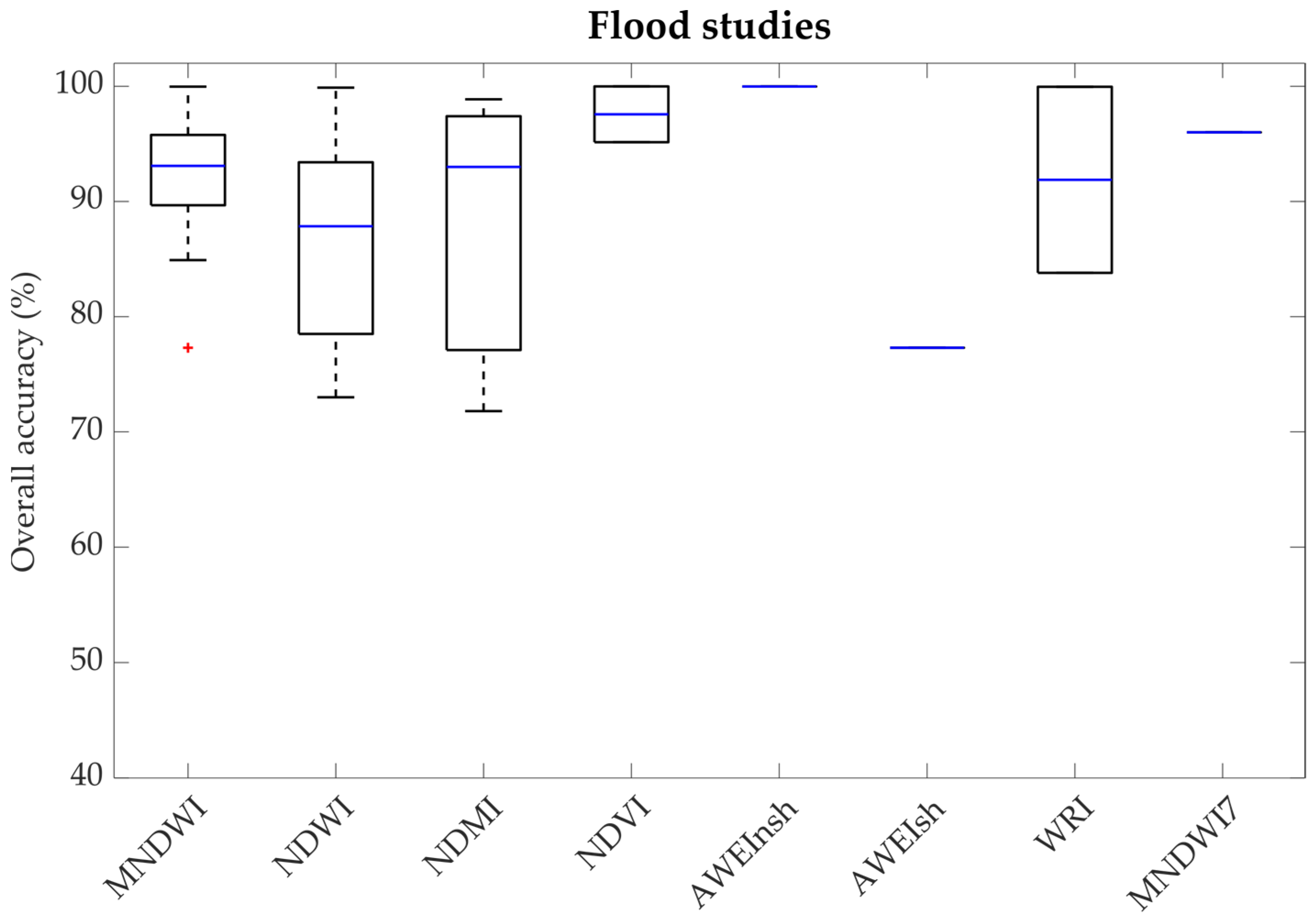
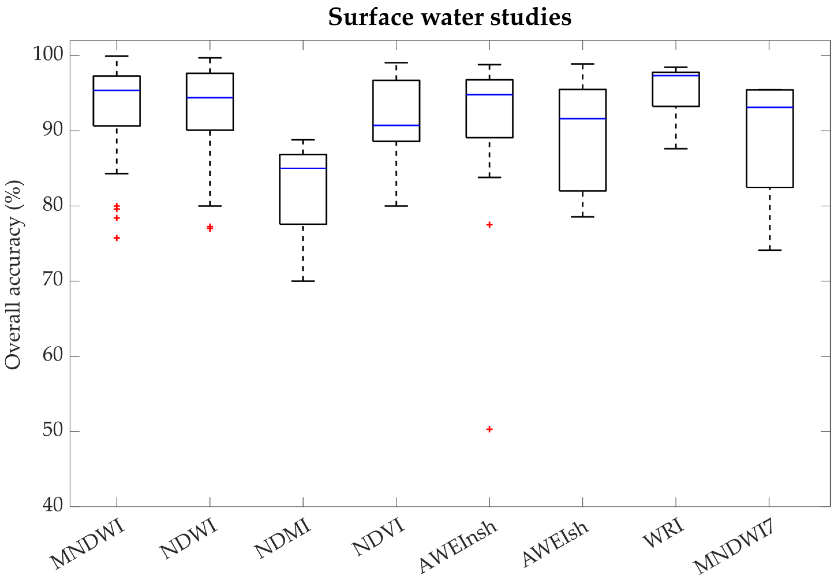
3.1. Performance Assessment

Thematic maps obtained from remote sensing data need to be verified in terms of quality, or accuracy, to check to which extent they correspond to reality. According to Stehman and Czaplewski [108], accuracy assessment follows a detailed protocol that includes three main components: (a) design of the reference sample, (b) response design to determine the reference classification, and (c) analysis of the classification accuracy through the estimation of error metrics.
The most common evaluation technique to perform an accuracy assessment of image classification (component c) of the assessment protocol is the confusion or error matrix, to be chosen as the standard method for checking the accuracy of remote sensing-derived maps [109]. A confusion matrix is the starting point for evaluation purposes in which the classified and reference maps are directly compared in a simple two-by-two table where diagonal values represent the number of correctly classified pixels, either true-positive (TP) or true-negative (TN) data, while off-diagonal values indicate misclassifications (i.e., false-positive (FP) and false-negative (FN) values). The confusion matrix allows several descriptive metrics to be computed, including the overall accuracy (OA), which describes the proportion of correctly classified pixels; the user’s accuracy (UA), also called reliability or precision, which describes the number of pixels assigned to class i that in fact correspond to that class in the reference image; and the producer’s accuracy (PA), also called sensitivity, recall, or true-positive rate, which represents the number of pixels corresponding to class j in the reference map and classified as class j in the classified image. In addition, the Kappa coefficient, κ , can be derived from the confusion matrix considering the overall proportion of agreement, p 0 , which corresponds to the overall accuracy, and the chance agreement, p c . This coefficient expresses the proportion of agreement between the classified and reference maps after removing the agreement that can occur by chance [110], and it also takes into consideration off-diagonal values. It ranges between −1 and 1, respectively indicating no or a perfect agreement, while a value equal to zero indicates agreement occurring by chance.
In general, surface water and flooded area delineation maps are in the form of binary images, in which pixels are either marked as water/flooded or non-water/non-flooded. Therefore, the confusion matrix is composed of two classes. Assuming that Table 4 is the result of a classification process for surface water detection and that the aim is to assess the accuracy of the derived water delineation map, the aforementioned descriptive statistics for the water class are expressed according to the formula reported in Equations (1)–(5).
O A   ( % ) = p 0 = T P + T N T · 100 ,
U A   ( % ) = T P C N W · 100 ,
P A   ( % ) = T P R W · 100 ,
p c ( % ) = ( R W · C W ) + ( R N W · C N W ) T 2 · 100 ,
κ = p 0 p c 100 p c ,
where T is the total number of pixels in the image and C W and C N W represent the total number of pixels respectively corresponding to water and non-water classes in the classified map, while R W and R N W represent the total number of pixels respectively corresponding to water and non-water classes in the reference map.

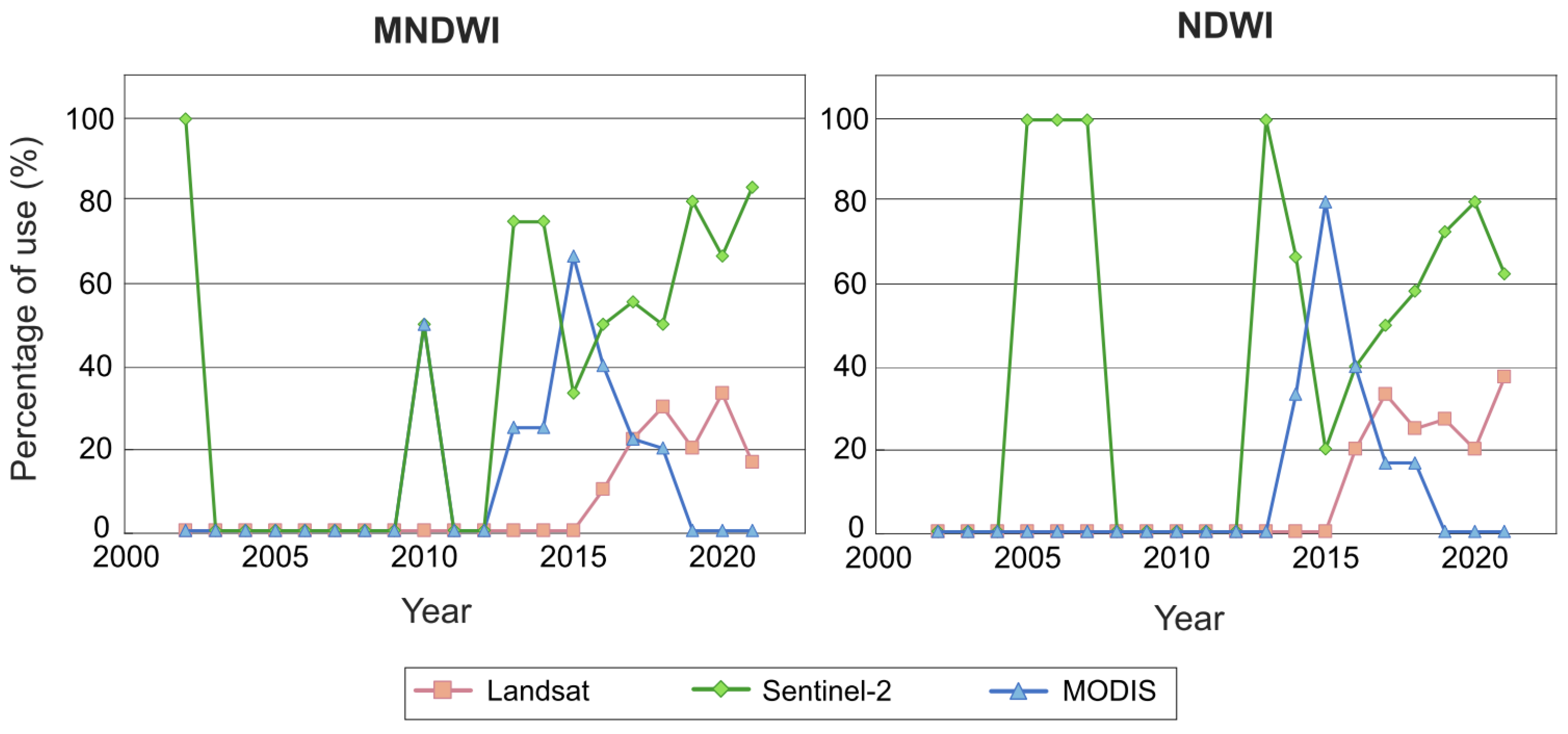
3.2. Investigation of Spectral Index Performances

In our investigation, we noticed that descriptive metrics are not always all used simultaneously to assess the performances of multispectral indices, with OA being the most commonly used. Therefore, to have a homogeneous and comparable metric among different studies, a further screening of the literature was necessary to take into consideration those that at least used OA as a performance metric. This was considered as a summary statistic for assessing the ability of the selected spectral indices to detect water pixels. The performance assessment was separately carried out for studies on flood mapping and surface water detection (i.e., water body mapping) that employed either Landsat 5-TM, Landsat 7-ETM+, Landsat 8, Sentinel-2, or MODIS or presented a comparison of more than one dataset. Among flooded area detection studies (42% of total studies), for example, Boschetti et al. [30] proposed a comparative analysis of several spectral indices to map flooded rice cropping systems using MODIS data. Validation on pure water pixels showed that among 11 selected indices, the best mapping accuracy was achieved by those based on the SWIR and visible bands, particularly the MNDWI (OA = 97%). Similarly, Munasinghe et al. [32] compared different inundation mapping methodologies, including supervised and unsupervised classification techniques, a change detection approach, and two spectral indices, i.e., the MNDWI and NDWI, based on Landsat 8-OLI satellite imagery. Despite the fact that other methods led to better performances, both indices achieved satisfactory results (OA values equal to 77.3% and 77.1% for the MNDWI and NDWI, respectively). Asmadin et al. [6] assessed the performances of seven water index algorithms, including, among others, the MNDWI, NDWI, NDMI, NDVI, and AWEInsh, derived from Sentinel-2A MSI and Landsat 8-OLI for coastal surface inundation mapping. In this case, indices from both sensors showed good accuracy (OA values above 94%). Using Sentinel-2 MSI data, Li et al. [111] performed an MNDWI-based segmentation to separate water and land features to ultimately characterize extreme flood impacts on the channel–floodplain morphology and sediment regime of the river system. The classification accuracy achieved 96%. More recently, Li et al. [94] combined Landsat images with precipitation data and high-resolution satellite imagery in the GEE environment to evaluate channel–floodplain dynamics. The authors used the MNDWI to extract the flooding extent, based on visual interpretation, achieving 93% of accuracy.
A higher number of studies that employed multispectral indices were found for surface water body detection (58% of total studies). One of the most significant works is the one proposed by Li et al. [112], in which Advanced Land Imagery (ALI) data and Landsat 5-TM and ETM+ images were selected to compare land surface water mapping based on the MNDWI, NDWI, and MNDWI7 in three different study sites. Despite the aim of the authors being to demonstrate the superiority of ALI data, Landsat imagery succeeded in delineating water features in all three regions. In particular, the indices based on the SWIR bands (i.e., the MNDWI and MNDWI7) showed very high and similar performances (OA values equal to 94.6% and 93.9% on average, respectively), while the accuracy of the NDWI was slightly lower (OA = 92% on average). Zhou et al. [29] evaluated the performances of six spectral indices, including the NDWI, MNDWI, AWEIsh, and AWEInsh, derived from three different sensors, i.e., Landsat 7-TM+, Landsat 8-OLI, and Sentinel-2 MSI, for water body mapping in Poyang Lake Basin, China. The authors showed the superiority of Landsat 8 and Sentinel-2 over Landsat 7 data and the higher performance of the NDWI in the selected study region (OA values equal to 95.7% and 95.6% for Landsat 8 and Sentinel-2, respectively). Ogilvie et al. [5] applied the spectral index segmentation method using Landsat imagery to map small lakes (from 1 to 30 ha) in Tunisia. The selected indices for validation purposes using Landsat 8 scenes of six different lakes included the MNDWI, NDWI, NDMI, and NDVI. The MNDWI had higher performances in four out of six cases (OA values above 89%), while in the other two sites, the NDWI and NDVI performed better (OA values equal to 80% and 88.1%, respectively).
To identify the best-performing spectral indices, we carefully analyzed the selected literature. No distinction was made among different satellite sensors, while accuracy values were evaluated separately for surface water detection and flooding extent delineation. The selected spectral indices for the performance assessment were the MNDWI, NDWI, NDMI, NDVI, AWEInsh, AWEIsh, WRI, and MNDWI7. We summarized the performances of each index with the boxplots reported in Figure 3 and Figure 4.
As regards flood mapping studies, the most used spectral indices were the MNDWI, NDWI, and NDMI (39.4%, 30.3%, and 9.1% of use among flood studies, respectively). Only two studies were found that employed the WRI and NDVI (12.2%) and one study that used the AWEInsh, AWEIsh, and MNDWI7 (9%). Figure 3 illustrates the performances of these indices expressed in terms of OA. Among the MNDWI, NDWI, and NDMI, the former was shown to be the best index both in terms of OA median value (93.03%), represented by the horizontal blue line in the box, and the spread of the data. The NDMI had a median value very close to that of the MNDWI (93%); however, the data were more spread out. The same occurred for values of the NDWI, whose median was equal to 87.85%.
Regarding surface water detection, the MNDWI and NDWI were the most common indices (27.8% and 26.4% of use among open water studies, respectively), followed by the AWEInsh (15.3%), NDVI (11.1%), AWEIsh (9.7%), WRI (4.2%), NDMI, and MNDWI7 (5.6%). Figure 4 illustrates the performances of these indices expressed in terms of OA. In this case, the MNDWI had an OA median value of 95.37% (horizontal blue line in the figure) and a relatively small spread of the data. However, some outliers were observed. The NDWI and AWEInsh had similar performances to those of the MNDWI, in terms of median value (94.41% and 94.80%, respectively), data spreading, and outlier values. The NDMI showed the lowest median value among all selected spectral indices (median OA value of 88.80%). Although the highest OA median value was observed for the WRI, only five studies were available, which may not be sufficient to satisfactory interpret its performance.
It is worthy to underline that the analyses presented herein did not consider the potential impact of the specific processing workflow adopted by each author. Therefore, there is a potential impact due to such methodologies that is hard to quantify, but we do believe that the overall analysis provides an interesting picture of the performances obtained by exploiting specific indices for the scope of interest.

3.3. Classification According to Land Cover

Multispectral remote sensing-derived indices allow flooded areas and water bodies to be quickly and effectively recognized. However, their performances can vary according to the land cover (i.e., crops, forests, and artificial surfaces), which influences the ability to discriminate between water and other features. To achieve a better understanding of multispectral applications and identify the spectral index that is best suited for a specific land cover setting, we qualitatively analyzed spectral index performances by classifying them according to different land cover types. In particular, the classification was carried out using the selected literature on flooded area mapping, by reviewing case studies and their land cover context, while land surface water detection studies clearly included only one class, i.e., water bodies. In addition, the analyses were carried out on the two spectral indices that showed the best performances in the previous assessment, i.e., the MNDWI and NDWI.
Most of the flood studies included regions in which agricultural areas constitute the main land cover type (e.g., [7,30,32,113]). Other studies were focused on regions mainly covered by forests (e.g., [94,111,114]), while only a few included urban areas or artificial surfaces and wetlands (e.g., [6,115]). Finally, some studies were carried out on the watershed scale (e.g., [8,29,116]); the performance metrics, thus, referred to the entire study area, and it was not possible to discriminate among land covers. For this reason, we considered three main classes to carry out a classification of the performances according to the land cover settings, namely, crops, forests, and mixed land. The latter indicate heterogeneous areas that include the contemporary presence of the first two classes, wetlands, urban areas, and/or artificial surfaces. Figure 5 shows the results of the accuracy evaluation of the MNDWI and NDWI for the three selected land cover categories. First, as highlighted above, the MNDWI showed better performances than the NDWI, both in terms of median values and data variation (left panel). Moreover, the MNDWI always showed the best performance in all three land cover categories (upper-right panel) compared with the NDWI in the same categories (lower-right panel). In terms of OA, the median values for the MNDWI were always above 93% for both crops and mixed lands (94.30% and 93.36%, respectively) and above 90% for forest areas (91.40%), while for the NDWI, values never exceeded 90%, with the highest value being observed in forests (88.70%) and the lowest in mixed land (85.98%). For croplands, the NDWI had an OA median value equal to 87%. As regards data variation, MNDWI values showed the lowest spread, while higher variation was observed for NDWI values, with the highest spread of mixed land data.
For comparison between MNDWI and NDWI performances in flooded area delineation, in Figure 6, the overall accuracy values of the same indices for land surface water detection are reported. As highlighted above, these two indices performed similarly in delineating water bodies; however, some outliers could be detected, mainly due to spatial resolution issues with respect to the water body surface area, turbidity of the water, mixed pixels, or shadows.

4. Discussion

In this work, an up-to-date review of remote sensing applications for water mapping was carried out focusing on satellite remote sensing programs that offer free-of-charge optical data. Several documents were carefully screened, and the relevant literature on flood mapping using multispectral imagery was included. To the authors’ knowledge, there is no similar scientific study focusing specifically on optical satellite imagery for flood mapping that also provides a review of spectral index performances in different flooded land cover classes. The most recent literature, in fact, has either focused on reviewing the use of optical data in the context of land cover classification [69] or on the application of radar data for inundation extent mapping [117,118]. Others have focused on global remote sensing satellites for land monitoring [70], Earth observations [34], and flood management [119].
The proposed review allowed us to summarize the actual knowledge on the use of multispectral remote sensing for flood and water body delineation and to directly compare the potential and limitations of different spectral indices adopted in water segmentation.
First, we analyzed the literature on flooded area and wetland inundation mapping with Landsat, MODIS, and Sentinel-2 satellite sensors in the period from 2002 to 2021. As expected, images from the Landsat program were the most used, since it constitutes the longest-running land monitoring program, offering a large dataset and allowing analyses to be conducted over several years. In addition, it offers medium–high resolution images (30–100 m spatial resolution), especially after the launch of the Landsat 7-ETM+ sensor. However, the revisit time is 16 days, thus limiting the possibility to have a frame of the flooded area at the exact moment of the event. Joining the Landsat 8 in orbit, the recent launch of the Landsat 9 satellite ensures a revisit coverage and data collection every 8 days. Sentinel-2 also belongs to the medium–high resolution class of satellite sensors (10 to 60 m spatial resolution) and has the advantage of having a 5-day revisit time; however, data are only available from 2015. Indeed, we found a relatively low number of studies that used Sentinel-2 images. Similarly, relevant studies that used data from the MODIS satellite were only found from 2008. Despite the coarse spatial resolution of the MODIS sensor (250 to 1000 m), it has the great advantage of a daily revisit time.
An in-depth investigation of the water index method for flooded area mapping and water body delineation was carried out, from which it was possible to identify the most used multispectral indices and assess their performances. The performance metric considered for the analysis was the overall accuracy, while the selected spectral indices were the MNDWI, NDWI, NDVI, NDMI, AWEInsh, AWEIsh, WRI, and MNDWI7. The results showed that the best-performing index for flooded area mapping was the MNDWI, thanks to its ability to better recognize mixed pixels and turbid water (i.e., algae and vegetation). As regards surface water detection, both the MNDWI and NDWI showed good performances; however, few outliers were detected. These were mainly found in study areas in which shadows represented a major issue, influencing MNDWI accuracy, while turbidity problems affected NDWI performance [2,26,84]. In addition, issues were also related to the spatial resolution of the sensor used to map the water bodies, which sometimes may have a limited size that is not easily visible with the current low spatial resolution of sensors (e.g., [5]). Other sources of errors were also represented by snow presence in the study area [27,120].
Difficulties in water segmentation can largely be connected to the presence of cloud cover and shadows, but this is not the only limiting factor. In fact, the ability of multispectral indices to reliably identify water features, especially flooded areas, can also be related to the land cover. Considering changes in land and vegetation coverage due to dynamic processes occurring during and after floods, the surface spectral reflectance can be affected. For this reason, we analyzed the overall accuracy values of the spectral indices according to three different land cover classes, i.e., crops, forests, and mixed areas. The results showed that for flood mapping, the MNDWI was found to be the best index in all the land cover settings, outperforming other indices especially in mixed lands, confirming its ability to discriminate mixed pixels. The comparison of the accuracy metrics from different research studies had the general purpose of providing further insight into the sensitivity of multispectral indices in detecting water features in different flooded land cover types. We are aware that such a comparison may suffer from some shortcomings, including the fact that validation methods of satellite-derived flood maps can vary from study to study and be based on different reference data (e.g., retrieved from satellite products themselves or ground-based), thus introducing a further source of error. Despite such limitations, the outcomes represent a potential reference to discriminate between different methods.
Our analyses included all the spectral indices used in flood mapping studies; however, good performances for detecting water areas could also be achieved using other vegetation indices, such as the Water-Adjusted Vegetation Index (WAVI). It was introduced by Villa [121] to retrieve information about aquatic vegetation and distinguish it from the terrestrial one. Applications also included the classification of macrophyte community types [122] and the detection of vegetation overgrowth processes in reservoirs [123]. Since aquatic vegetation relies on the presence of water, the application of WAVI for flood mapping studies can have some good potential, not yet explored in the literature.
The accuracy of water extraction methods, the thresholds for image classification, and the interpretation of results may differ based on the pre-processing chain adopted to solve issues related, for example, to sensor, atmospheric, and geometric noises [2,105]. Optical imagery, in fact, needs a proper pre-processing stage prior the calculation of water indices, especially if the available products are in the form of raw DN values. A typical workflow to pre-process remote sensing data includes radiometric calibration (to convert DNs to at-sensor spectral radiance, i.e., Top Of Atmosphere - TOA) and atmospheric corrections (to convert at-sensor radiance to at-surface reflectance, i.e., Bottom of Atmosphere - BOA). In particular, radiometrically and atmospherically corrected Landsat images are frequently obtained by applying tools available in ENVI image analysis software, such as the Radiometric Calibration tool and the Fast Line-of-Sight Atmospheric Analysis of Spectral Hyper-cube (FLAASH) module (e.g., [4,31,67,105,124]), while for Sentinel-2 data water detection approaches are directly applied to level 1C (TOA products, e.g., [125]) or 2A (BOA products, e.g., [111]). It is worth noting that the investigation of the specific pre-processing workflow adopted in each work considered in our analyses was not within the scope of the present manuscript. Nevertheless, the influence of such methods on the water index accuracy values requires more in-depth investigations.

5. Conclusions

Optical satellites represent a straightforward instrument for flooded area and water body mapping. In fact, the multi-band sensors allow the spectral signatures of different objects to be exploited and information to be derived through a direct visual interpretation of scenes of specific bands or color composites. In addition, multispectral imagery allows information about river morphology dynamics and land cover changes to be integrated in flood risk modelling and provides good spatial resolution for flood management applications, although with some limitations. The proposed analyses had the more general aims of identifying sensors and methods most used and best suited for monitoring water-related processes, highlighting the potentials of spectral indices, and providing some general practical guidance for targeted applications in different contexts. We believe that this could be beneficial not only for satellite-based remote sensing but also for UAS-based environmental monitoring, which in addition allows the cloud cover issue that affects optical remote sensing to be overcome. The analyses presented here can, indeed, be transferred to airborne-based applications to identify the best methodology that can ensure a reliable flood-prone area delineation using multispectral sensors. The opportunities offered by UAS technology are not only related to the possibility of flying below cloud cover layers and vegetation canopies, as it also enables submeter-level spatial resolution acquisition necessary for a detailed understanding of flood processes (see [9]). On the other hand, UASs have the limitation of not being able to survey vast areas. Although this issue could be overcome with multipleUASs flying simultaneously over the same area, proper regulations that allow multi-UAS flight to be performed are still lacking. Nevertheless, the potentiality offered by such a system represents a versatile support to satellite imagery.
Promising applications of passive remote sensing under cloud conditions are also those from the CYGNSS constellation, which presents the advantages of similar microwave sensors (such as Synthetic Aperture Radar (SAR)) of seeing through clouds but at higher temporal resolutions. New-generation passive satellites are, in fact, characterized by a higher revisit time over land and ocean, which increases the chance to have closer post-flood observations. The aforementioned CYGNSS is one example, but valuable applications, still at their dawn, are also those offered, for example, by the family of small satellites of CubeSat. Although suffering from cloud cover problems, as with optical data, it provides both high-temporal (nearly daily)- and -spatial-resolution (~3 m) multispectral imagery on the global scale [126,127,128].
Future research directions should expand the unprecedent opportunities offered by the new generation of passive satellites, which could be enhanced by merging data from multiple sources, thus combining the potential of multispectral imagery at high temporal resolution (e.g., CubeSat data) with the capabilities of radar data (e.g., CYGNSS). Moreover, hybrid approaches, also including NOAA AVHRR data, which increase the possibility of obtaining cloud-free data, could also be explored. Finally, the advent of emerging technologies such as hyperspectral imagery (e.g., the recently launched Environmental Mapping and Analysis Program (EnMAP) German satellite) offers the possibility to better discriminate the spectral signature of different surfaces (thanks to the many different spectral bands) and to be used in conjunction with multispectral data, allowing detailed information to be retrieved, which is not achievable with multispectral data alone. Regarding multispectral indices, future opportunities can be represented by the application of the WAVI in flood mapping studies.
In conclusion, both optical and passive microwave satellite sensors will likely continue to represent a reference for Earth imaging applications, enabling a better understanding of surface water dynamics. Indeed, European Union’s Earth Observation Copernicus Programme makes a large use of these remote sensing technologies for monitoring the Earth’s surface and supply operational products (e.g., the free-of-charge flood maps produced by the Rapid Mapping module of Copernicus Emergency Management Service (CEMS)) to the end-user community [129].

Author Contributions

Writing—original draft preparation, C.A.; writing—review and editing, C.A., S.M., A.G. and V.I.; supervision, S.M., A.G. and V.I. All authors have read and agreed to the published version of the manuscript.

Funding

This research was supported by the COST Action CA16219 “HARMONIOUS—Harmonization of UAS techniques for agricultural and natural ecosystems monitoring”.

Conflicts of Interest

The authors declare no conflict of interest.

References

  1. Schumann, G.J.-P.; Brakenridge, G.R.; Kettner, A.J.; Kashif, R.; Niebuhr, E. Assisting Flood Disaster Response with Earth Observation Data and Products: A Critical Assessment. Remote Sens. 2018, 10, 1230. [Google Scholar] [CrossRef] [Green Version]
  2. Buma, W.G.; Lee, S.-I.; Seo, J.Y. Recent Surface Water Extent of Lake Chad from Multispectral Sensors and GRACE. Sensors 2018, 18, 2082. [Google Scholar] [CrossRef] [PubMed] [Green Version]
  3. Liu, D.; Li, Y. Extraction of Water-Body in Remote Sensing Image Based on Logic Operation. In Proceedings of the 2011 19th International Conference on Geoinformatics, Shanghai, China, 24–26 June 2011; pp. 1–4. [Google Scholar]
  4. Rokni, K.; Ahmad, A.; Selamat, A.; Hazini, S. Water Feature Extraction and Change Detection Using Multitemporal Landsat Imagery. Remote Sens. 2014, 6, 4173–4189. [Google Scholar] [CrossRef] [Green Version]
  5. Ogilvie, A.; Belaud, G.; Massuel, S.; Mulligan, M.; Le Goulven, P.; Calvez, R. Surface Water Monitoring in Small Water Bodies: Potential and Limits of Multi-Sensor Landsat Time Series. Hydrol. Earth Syst. Sci. 2018, 22, 4349–4380. [Google Scholar] [CrossRef] [Green Version]
  6. Asmadin; Siregar, V.P.; Sofian, I.; Jaya, I.; Wijanarto, A.B. Feature Extraction of Coastal Surface Inundation via Water Index Algorithms Using Multispectral Satellite on North Jakarta. IOP Conf. Ser. Earth Environ. Sci. 2018, 176, 12032. [Google Scholar] [CrossRef]
  7. Ireland, G.; Volpi, M.; Petropoulos, G.P. Examining the Capability of Supervised Machine Learning Classifiers in Extracting Flooded Areas from Landsat TM Imagery: A Case Study from a Mediterranean Flood. Remote Sens. 2015, 7, 3372–3399. [Google Scholar] [CrossRef] [Green Version]
  8. Memon, A.A.; Muhammad, S.; Rahman, S.; Haq, M. Flood Monitoring and Damage Assessment Using Water Indices: A Case Study of Pakistan Flood-2012. Egypt. J. Remote Sens. Space Sci. 2015, 18, 99–106. [Google Scholar] [CrossRef] [Green Version]
  9. Manfreda, S.; Ben Dor, E. Unmanned Aerial Systems for Monitoring Soil, Vegetation, and Riverine Environments, Earth Observation Series, 1st ed.; Elsevier: Amsterdam, The Netherlands, 2023; ISBN 9780323852838. [Google Scholar]
  10. Manfreda, S.; McCabe, M.F.; Miller, P.E.; Lucas, R.; Madrigal, V.P.; Mallinis, G.; Dor, E.B.; Helman, D.; Estes, L.; Ciraolo, G.; et al. On the Use of Unmanned Aerial Systems for Environmental Monitoring. Remote Sens. 2018, 10, 641. [Google Scholar] [CrossRef] [Green Version]
  11. Chew, C.; Reager, J.T.; Small, E. CYGNSS Data Map Flood Inundation during the 2017 Atlantic Hurricane Season. Sci. Rep. 2018, 8, 9336. [Google Scholar] [CrossRef]
  12. Wan, W.; Liu, B.; Zeng, Z.; Chen, X.; Wu, G.; Xu, L.; Chen, X.; Hong, Y. Using CYGNSS Data to Monitor China’s Flood Inundation during Typhoon and Extreme Precipitation Events in 2017. Remote Sens. 2019, 11, 854. [Google Scholar] [CrossRef]
  13. Gerlein-Safdi, C.; Ruf, C.S. A CYGNSS-Based Algorithm for the Detection of Inland Waterbodies. Geophys. Res. Lett. 2019, 46, 12065–12072. [Google Scholar] [CrossRef]
  14. Chew, C.; Small, E. Estimating Inundation Extent Using CYGNSS Data: A Conceptual Modeling Study. Remote Sens. Environ. 2020, 246, 111869. [Google Scholar] [CrossRef]
  15. Rajabi, M.; Nahavandchi, H.; Hoseini, M. Evaluation of CYGNSS Observations for Flood Detection and Mapping during Sistan and Baluchestan Torrential Rain in 2020. Water 2020, 12, 2047. [Google Scholar] [CrossRef]
  16. Zhang, S.; Ma, Z.; Li, Z.; Zhang, P.; Liu, Q.; Nan, Y.; Zhang, J.; Hu, S.; Feng, Y.; Zhao, H. Using CYGNSS Data to Map Flood Inundation during the 2021 Extreme Precipitation in Henan Province, China. Remote Sens. 2021, 13, 5181. [Google Scholar] [CrossRef]
  17. Ruf, C.S.; Chew, C.; Lang, T.; Morris, M.G.; Nave, K.; Ridley, A.; Balasubramaniam, R. A New Paradigm in Earth Environmental Monitoring with the CYGNSS Small Satellite Constellation. Sci. Rep. 2018, 8, 8782. [Google Scholar] [CrossRef] [Green Version]
  18. Boothroyd, R.J.; Nones, M.; Guerrero, M. Deriving Planform Morphology and Vegetation Coverage from Remote Sensing to Support River Management Applications. Front. Environ. Sci. 2021, 9, 657354. [Google Scholar] [CrossRef]
  19. Henshaw, A.J.; Gurnell, A.M.; Bertoldi, W.; Drake, N.A. An Assessment of the Degree to Which Landsat TM Data Can Support the Assessment of Fluvial Dynamics, as Revealed by Changes in Vegetation Extent and Channel Position, along a Large River. Geomorphology 2013, 202, 74–85. [Google Scholar] [CrossRef]
  20. Cavallo, C.; Papa, M.N.; Gargiulo, M.; Palau-Salvador, G.; Vezza, P.; Ruello, G. Continuous Monitoring of the Flooding Dynamics in the Albufera Wetland (Spain) by Landsat-8 and Sentinel-2 Datasets. Remote Sens. 2021, 13, 3525. [Google Scholar] [CrossRef]
  21. Soomro, S.; Hu, C.; Boota, M.W.; Soomro, M.H.A.A.; Jian, S.; Zafar, Z.; Li, X. Mapping Flood Extend and Its Impact on Land Use/Land Cover and Settlements Variations: A Case Study of Layyah District, Punjab, Pakistan. Acta Geophys. 2021, 69, 2291–2304. [Google Scholar] [CrossRef]
  22. Radice, A.; Rosatti, G.; Ballio, F.; Franzetti, S.; Mauri, M.; Spagnolatti, M.; Garegnani, G. Management of Flood Hazard via Hydro-Morphological River Modelling. The Case of the Mallero in Italian Alps. J. Flood Risk Manag. 2013, 6, 197–209. [Google Scholar] [CrossRef]
  23. Bertoldi, W.; Drake, N.A.; Gurnell, A.M. Interactions between River Flows and Colonizing Vegetation on a Braided River: Exploring Spatial and Temporal Dynamics in Riparian Vegetation Cover Using Satellite Data. Earth Surf. Process. Landf. 2011, 36, 1474–1486. [Google Scholar] [CrossRef]
  24. Gurnell, A.M. Trees, Wood and River Morphodynamics: Results from 15 Years Research on the Tagliamento River, Italy. In River Science: Research and Management for the 21st Century; Gilvear, D.J., Greenwood, M.T., Thoms, M.C., Wood, P.J., Eds.; John Wiley & Sons: Chichester, UK, 2016; pp. 132–155. [Google Scholar] [CrossRef]
  25. Masocha, M.; Dube, T.; Makore, M.; Shekede, M.D.; Funani, J. Surface Water Bodies Mapping in Zimbabwe Using Landsat 8 OLI Multispectral Imagery: A Comparison of Multiple Water Indices. Phys. Chem. Earth Parts A/B/C 2018, 106, 63–67. [Google Scholar] [CrossRef]
  26. Xu, H. Modification of Normalised Difference Water Index (NDWI) to Enhance Open Water Features in Remotely Sensed Imagery. Int. J. Remote Sens. 2006, 27, 3025–3033. [Google Scholar] [CrossRef]
  27. Khalid, H.W.; Khalil, R.M.Z.; Qureshi, M.A. Evaluating Spectral Indices for Water Bodies Extraction in Western Tibetan Plateau. Egypt. J. Remote Sens. Space Sci. 2021, 24, 619–634. [Google Scholar] [CrossRef]
  28. Parihar, S.K.; Borana, S.L.; Yadav, S.K. Comparative Evaluation of Spectral Indices and Sensors for Mapping of Urban Surface Water Bodies in Jodhpur Area: Smart & Sustainable Growth. In Proceedings of the 2019 International Conference on Computing, Communication, and Intelligent Systems (ICCCIS), Greater Noida, India, 18–19 October 2019; pp. 484–489. [Google Scholar] [CrossRef]
  29. Zhou, S.L.; Zhang, W.C. Flood Monitoring and Damage Assessment in Thailand Using Multi-Temporal HJ-1A/1B and MODIS Images. In IOP Conference Series: Earth and Environmental Science; IOP Publishing: Bristol, UK, 2017; Volume 57, p. 12016. [Google Scholar] [CrossRef]
  30. Boschetti, M.; Nutini, F.; Manfron, G.; Brivio, P.A.; Nelson, A. Comparative Analysis of Normalised Difference Spectral Indices Derived from MODIS for Detecting Surface Water in Flooded Rice Cropping Systems. PLoS ONE 2014, 9, e88741. [Google Scholar] [CrossRef] [PubMed]
  31. Chiloane, C.; Dube, T.; Shoko, C. Monitoring and Assessment of the Seasonal and Inter-Annual Pan Inundation Dynamics in the Kgalagadi Transfrontier Park, Southern Africa. Phys. Chem. Earth Parts A/B/C 2020, 118, 102905. [Google Scholar] [CrossRef]
  32. Munasinghe, D.; Cohen, S.; Huang, Y.; Tsang, Y.; Zhang, J.; Fang, Z. Intercomparison of Satellite Remote Sensing-Based Flood Inundation Mapping Techniques. JAWRA J. Am. Water Resour. Assoc. 2018, 54, 834–846. [Google Scholar] [CrossRef]
  33. Rouse, J.W.; Haas, R.H.; Schell, J.A.; Deering, D.W. Monitoring Vegetation Systems in the Great Plains with ERTS (Earth Resources Technology Satellite). In Proceedings of the Third Earth Resources Technology Satellite Symposium, Greenbelt, ON, Canada, 10–14 December 1973; Volume SP-351, pp. 309–317. [Google Scholar]
  34. McFeeters, S.K. The Use of the Normalized Difference Water Index (NDWI) in the Delineation of Open Water Features. Int. J. Remote Sens. 1996, 17, 1425–1432. [Google Scholar] [CrossRef]
  35. Notti, D.; Giordan, D.; Caló, F.; Pepe, A.; Zucca, F.; Galve, J.P. Potential and Limitations of Open Satellite Data for Flood Mapping. Remote Sens. 2018, 10, 1673. [Google Scholar] [CrossRef] [Green Version]
  36. U.S. Geological Survey (USGS) EarthExplorer. Available online: https://earthexplorer.usgs.gov/ (accessed on 4 February 2022).
  37. Sentinel Scientific Data Hub. Available online: https://scihub.copernicus.eu/ (accessed on 4 February 2022).
  38. Earthdata Search—NASA. Available online: https://search.earthdata.nasa.gov/search (accessed on 4 February 2022).
  39. LAADS DAAC. Available online: https://ladsweb.modaps.eosdis.nasa.gov/ (accessed on 4 February 2022).
  40. Zhao, Q.; Yu, L.; Du, Z.; Peng, D.; Hao, P.; Zhang, Y.; Gong, P. An Overview of the Applications of Earth Observation Satellite Data: Impacts and Future Trends. Remote Sens. 2022, 14, 1863. [Google Scholar] [CrossRef]
  41. Chignell, S.M.; Anderson, R.S.; Evangelista, P.H.; Laituri, M.J.; Merritt, D.M. Multi-Temporal Independent Component Analysis and Landsat 8 for Delineating Maximum Extent of the 2013 Colorado Front Range Flood. Remote Sens. 2015, 7, 9822–9843. [Google Scholar] [CrossRef] [Green Version]
  42. Ghansah, B.; Nyamekye, C.; Owusu, S.; Agyapong, E. Mapping Flood Prone and Hazards Areas in Rural Landscape Using Landsat Images and Random Forest Classification: Case Study of Nasia Watershed in Ghana. Cogent Eng. 2021, 8, 1923384. [Google Scholar] [CrossRef]
  43. Hudson, P.F.; Colditz, R.R. Flood Delineation in a Large and Complex Alluvial Valley, Lower Panuco Basin, Mexico. J. Hydrol. 2003, 280, 229–245. [Google Scholar] [CrossRef]
  44. Jung, H.C.; Alsdorf, D.; Moritz, M.; Lee, H.; Vassolo, S. Analysis of the Relationship between Flooding Area and Water Height in the Logone Floodplain. Phys. Chem. Earth Parts A/B/C 2011, 36, 232–240. [Google Scholar] [CrossRef]
  45. Nandi, I.; Srivastava, P.K.; Shah, K. Floodplain Mapping through Support Vector Machine and Optical/Infrared Images from Landsat 8 OLI/TIRS Sensors: Case Study from Varanasi. Water Resour. Manag. 2017, 31, 1157–1171. [Google Scholar] [CrossRef]
  46. Thomas, R.F.; Kingsford, R.T.; Lu, Y.; Hunter, S.J. Landsat Mapping of Annual Inundation (1979–2006) of the Macquarie Marshes in Semi-Arid Australia. Int. J. Remote Sens. 2011, 32, 4545–4569. [Google Scholar] [CrossRef]
  47. Thomas, R.F.; Kingsford, R.T.; Lu, Y.; Cox, S.J.; Sims, N.C.; Hunter, S.J. Mapping Inundation in the Heterogeneous Floodplain Wetlands of the Macquarie Marshes, Using Landsat Thematic Mapper. J. Hydrol. 2015, 524, 194–213. [Google Scholar] [CrossRef]
  48. Thito, K.; Wolski, P.; Murray-Hudson, M. Mapping Inundation Extent, Frequency and Duration in the Okavango Delta from 2001 to 2012. Afr. J. Aquat. Sci. 2016, 41, 267–277. [Google Scholar] [CrossRef]
  49. Amarnath, G.; Ameer, M.; Aggarwal, P.; Smakhtin, V. Detecting Spatio-Temporal Changes in the Extent of Seasonal and Annual Flooding in South Asia Using Multi-Resolution Satellite Data. In Earth Resources and Environmental Remote Sensing/GIS Applications III: Proceedings of the International Society for Optics and Photonics (SPIE), Volume 8538, Amsterdam, The Netherland, 1–6 July 2012; International Society for Optics and Photonics (SPIE): Bellingham, WA, USA, 2012; p. 853818. [Google Scholar] [CrossRef]
  50. Islam, A.S.; Bala, S.K.; Haque, M.A. Flood Inundation Map of Bangladesh Using MODIS Time-series Images. J. Flood Risk Manag. 2010, 3, 210–222. [Google Scholar] [CrossRef]
  51. Ogilvie, A.; Belaud, G.; Delenne, C.; Bailly, J.-S.; Bader, J.-C.; Oleksiak, A.; Ferry, L.; Martin, D. Decadal Monitoring of the Niger Inner Delta Flood Dynamics Using MODIS Optical Data. J. Hydrol. 2015, 523, 368–383. [Google Scholar] [CrossRef] [Green Version]
  52. Timár, G.; Székely, B.; Molnár, G.; Ferencz, C.; Kern, A.; Galambos, C.; Gercsák, G.; Zentai, L. Combination of Historical Maps and Satellite Images of the Banat Region—Re-Appearance of an Old Wetland Area. Glob. Planet. Chang. 2008, 62, 29–38. [Google Scholar] [CrossRef]
  53. Kordelas, G.A.; Manakos, I.; Aragonés, D.; Díaz-Delgado, R.; Bustamante, J. Fast and Automatic Data-Driven Thresholding for Inundation Mapping with Sentinel-2 Data. Remote Sens. 2018, 10, 910. [Google Scholar] [CrossRef] [Green Version]
  54. Kordelas, G.A.; Manakos, I.; Lefebvre, G.; Poulin, B. Automatic Inundation Mapping Using Sentinel-2 Data Applicable to Both Camargue and Doñana Biosphere Reserves. Remote Sens. 2019, 11, 2251. [Google Scholar] [CrossRef] [Green Version]
  55. Ludwig, C.; Walli, A.; Schleicher, C.; Weichselbaum, J.; Riffler, M. A Highly Automated Algorithm for Wetland Detection Using Multi-Temporal Optical Satellite Data. Remote Sens. Environ. 2019, 224, 333–351. [Google Scholar] [CrossRef]
  56. Solovey, T. Flooded Wetlands Mapping from Sentinel-2 Imagery with Spectral Water Index: A Case Study of Kampinos National Park in Central Poland. Geol. Q. 2020, 64, 492–505. [Google Scholar] [CrossRef] [Green Version]
  57. Li, L.; Xu, T.; Chen, Y. Improved Urban Flooding Mapping from Remote Sensing Images Using Generalized Regression Neural Network-Based Super-Resolution Algorithm. Remote Sens. 2016, 8, 625. [Google Scholar] [CrossRef]
  58. Li, L.; Chen, Y.; Xu, T.; Meng, L.; Huang, C.; Shi, K. Spatial Attraction Models Coupled with Elman Neural Networks for Enhancing Sub-Pixel Urban Inundation Mapping. Remote Sens. 2020, 12, 2068. [Google Scholar] [CrossRef]
  59. Colditz, R.R.; Souza, C.T.; Vazquez, B.; Wickel, A.J.; Ressl, R. Analysis of Optimal Thresholds for Identification of Open Water Using MODIS-Derived Spectral Indices for Two Coastal Wetland Systems in Mexico. Int. J. Appl. Earth Obs. Geoinf. 2018, 70, 13–24. [Google Scholar] [CrossRef]
  60. Yan, Y.-E.; Ouyang, Z.-T.; Guo, H.-Q.; Jin, S.-S.; Zhao, B. Detecting the Spatiotemporal Changes of Tidal Flood in the Estuarine Wetland by Using MODIS Time Series Data. J. Hydrol. 2010, 384, 156–163. [Google Scholar] [CrossRef]
  61. Wang, Y. Using Landsat 7 TM Data Acquired Days after a Flood Event to Delineate the Maximum Flood Extent on a Coastal Floodplain. Int. J. Remote Sens. 2004, 25, 959–974. [Google Scholar] [CrossRef]
  62. Wang, Y.; Colby, J.D.; Mulcahy, K.A. An Efficient Method for Mapping Flood Extent in a Coastal Floodplain Using Landsat TM and DEM Data. Int. J. Remote Sens. 2002, 23, 3681–3696. [Google Scholar] [CrossRef]
  63. Atif, I.; Mahboob, M.A.; Waheed, A. Spatio-Temporal Mapping and Multi-Sector Damage Assessment of 2014 Flood in Pakistan Using Remote Sensing and GIS. Indian J. Sci. Technol. 2015, 8, 1–9. [Google Scholar] [CrossRef]
  64. Cuca, B.; Barazzetti, L. Damages from Extreme Flooding Events to Cultural Heritage and Landscapes: Water Component Estimation for Centa River (Albenga, Italy). Adv. Geosci. 2018, 45, 389–395. [Google Scholar] [CrossRef] [Green Version]
  65. Gianinetto, M.; Villa, P.; Lechi, G. Postflood Damage Evaluation Using Landsat TM and ETM+ Data Integrated with DEM. IEEE Trans. Geosci. Remote Sens. 2005, 44, 236–243. [Google Scholar] [CrossRef]
  66. Haq, M.; Akhtar, M.; Muhammad, S.; Paras, S.; Rahmatullah, J. Techniques of Remote Sensing and GIS for Flood Monitoring and Damage Assessment: A Case Study of Sindh Province, Pakistan. Egypt. J. Remote Sens. Space Sci. 2012, 15, 135–141. [Google Scholar] [CrossRef] [Green Version]
  67. Sajjad, A.; Lu, J.; Chen, X.; Chisenga, C.; Saleem, N.; Hassan, H. Operational Monitoring and Damage Assessment of Riverine Flood-2014 in the Lower Chenab Plain, Punjab, Pakistan, Using Remote Sensing and GIS Techniques. Remote Sens. 2020, 12, 714. [Google Scholar] [CrossRef]
  68. Villa, P.; Gianinetto, M. Multispectral Transform and Spline Interpolation for Mapping Flood Damages. In Proceedings of the 2006 IEEE International Symposium on Geoscience and Remote Sensing, Denver, CO, USA, 31 July–4 August 2006; pp. 275–278. [Google Scholar] [CrossRef]
  69. Gómez, C.; White, J.C.; Wulder, M.A. Optical Remotely Sensed Time Series Data for Land Cover Classification: A Review. ISPRS J. Photogramm. Remote Sens. 2016, 116, 55–72. [Google Scholar] [CrossRef] [Green Version]
  70. Radočaj, D.; Obhođaš, J.; Jurišić, M.; Gašparović, M. Global Open Data Remote Sensing Satellite Missions for Land Monitoring and Conservation: A Review. Land 2020, 9, 402. [Google Scholar] [CrossRef]
  71. Foroughnia, F.; Alfieri, S.M.; Menenti, M.; Lindenbergh, R. Evaluation of SAR and Optical Data for Flood Delineation Using Supervised and Unsupervised Classification. Remote Sens. 2022, 14, 3718. [Google Scholar] [CrossRef]
  72. Sims, N.C.; Thoms, M.C. What Happens When Flood Plains Wet Themselves: Vegetation Response to Inundation on the Lower. In Proceedings of the Structure, Function and Management Implications of Fluvial Sedimentary Systems, Alice Springs, Australia, 2–6 September 2002; p. 195. [Google Scholar]
  73. Frazier, P.; Page, K. A Reach-scale Remote Sensing Technique to Relate Wetland Inundation to River Flow. River Res. Appl. 2009, 25, 836–849. [Google Scholar] [CrossRef]
  74. Otsu, N. A Threshold Selection Method from Gray-Level Histograms. IEEE Trans. Syst. Man Cybern. 1979, 9, 62–66. [Google Scholar] [CrossRef] [Green Version]
  75. Demirkesen, A.C.; Evrendilek, F.; Berberoglu, S.; Kilic, S. Coastal Flood Risk Analysis Using Landsat-7 ETM+ Imagery and SRTM DEM: A Case Study of Izmir, Turkey. Environ. Monit. Assess. 2007, 131, 293–300. [Google Scholar] [CrossRef] [PubMed]
  76. Esfandiari, M.; Jabari, S.; McGrath, H.; Coleman, D. Flood mapping using random forest and identifying the essential conditioning factors: A case study in Fredericton, New Brunswick, Canada. ISPRS Ann. Photogramm. Remote Sens. Spat. Inf. Sci. 2020, V–3–2020, 609–615. [Google Scholar] [CrossRef]
  77. Farhadi, H.; Najafzadeh, M. Flood Risk Mapping by Remote Sensing Data and Random Forest Technique. Water 2021, 13, 3115. [Google Scholar] [CrossRef]
  78. Tulbure, M.G.; Broich, M.; Stehman, S.V.; Kommareddy, A. Surface Water Extent Dynamics from Three Decades of Seasonally Continuous Landsat Time Series at Subcontinental Scale in a Semi-Arid Region. Remote Sens. Environ. 2016, 178, 142–157. [Google Scholar] [CrossRef]
  79. Dey, C.; Jia, X.; Fraser, D.; Wang, L. Mixed Pixel Analysis for Flood Mapping Using Extended Support Vector Machine. In Proceedings of the 2009 Digital Image Computing: Techniques and Applications, Melbourne, Australia, 1–3 December 2009; pp. 291–295. [Google Scholar] [CrossRef] [Green Version]
  80. Zhang, R.; Sun, D.; Yu, Y.; Goldberg, M.D. Mapping Nighttime Flood from MODIS Observations Using Support Vector Machines. Photogramm. Eng. Remote Sens. 2012, 78, 1151–1161. [Google Scholar] [CrossRef]
  81. Ball, G.H.; Hall, D.J. ISODATA, a Novel Method of Data Analysis and Pattern Classification; Stanford Research Institute: Menlo Park, CA, USA, 1965. [Google Scholar]
  82. Jung, Y.; Kim, D.; Kim, D.; Kim, M.; Lee, S.O. Simplified Flood Inundation Mapping Based on Flood Elevation-Discharge Rating Curves Using Satellite Images in Gauged Watersheds. Water 2014, 6, 1280–1299. [Google Scholar] [CrossRef]
  83. Ho, L.T.K.; Umitsu, M.; Yamaguchi, Y. Flood Hazard Mapping by Satellite Images and SRTM DEM in the Vu Gia-Thu Bon Alluvial Plain, Central Vietnam. Int. Arch. Photogramm. Remote Sens. Spat. Inf. Sci. 2010, 38, 275–280. [Google Scholar]
  84. Kumar, R.; Acharya, P. Flood Hazard and Risk Assessment of 2014 Floods in Kashmir Valley: A Space-Based Multisensor Approach. Nat. Hazard. 2016, 84, 437–464. [Google Scholar] [CrossRef]
  85. Kwak, Y.; Park, J.; Fukami, K. Estimating Floodwater from MODIS Time Series and SRTM DEM Data. Artif. Life Robot. 2014, 19, 95–102. [Google Scholar] [CrossRef]
  86. Nobre, A.D.; Cuartas, L.A.; Momo, M.R.; Severo, D.L.; Pinheiro, A.; Nobre, C.A. HAND Contour: A New Proxy Predictor of Inundation Extent. Hydrol. Process. 2016, 30, 320–333. [Google Scholar] [CrossRef]
  87. Manfreda, S.; Samela, C.; Gioia, A.; Consoli, G.G.; Iacobellis, V.; Giuzio, L.; Cantisani, A.; Sole, A. Flood-Prone Areas Assessment Using Linear Binary Classifiers Based on Flood Maps Obtained from 1D and 2D Hydraulic Models. Nat. Hazard. 2015, 79, 735–754. [Google Scholar] [CrossRef]
  88. Samela, C.; Troy, T.J.; Manfreda, S. Geomorphic Classifiers for Flood-Prone Areas Delineation for Data-Scarce Environments. Adv. Water Resour. 2017, 102, 13–28. [Google Scholar] [CrossRef]
  89. Totaro, V.; Peschechera, G.; Gioia, A.; Iacobellis, V.; Fratino, U. Comparison of Satellite and Geomorphic Indices for Flooded Areas Detection in a Mediterranean River Basin. In Proceedings of the International Conference on Computational Science and Its Applications—ICCSA 2019, Saint Petersburg, Russia, 1–4 July 2019; Springer International Publishing: Cham, Switzerland, 2019; pp. 173–185. [Google Scholar]
  90. Mehmood, H.; Conway, C.; Perera, D. Mapping of Flood Areas Using Landsat with Google Earth Engine Cloud Platform. Atmosphere 2021, 12, 866. [Google Scholar] [CrossRef]
  91. Gorelick, N.; Hancher, M.; Dixon, M.; Ilyushchenko, S.; Thau, D.; Moore, R. Google Earth Engine: Planetary-Scale Geospatial Analysis for Everyone. Remote Sens. Environ. 2017, 202, 18–27. [Google Scholar] [CrossRef]
  92. Hardy, A.; Oakes, G.; Ettritch, G. Tropical Wetland (TropWet) Mapping Tool: The Automatic Detection of Open and Vegetated Waterbodies in Google Earth Engine for Tropical Wetlands. Remote Sens. 2020, 12, 1182. [Google Scholar] [CrossRef] [Green Version]
  93. Inman, V.L.; Lyons, M.B. Automated Inundation Mapping over Large Areas Using Landsat Data and Google Earth Engine. Remote Sens. 2020, 12, 1348. [Google Scholar] [CrossRef] [Green Version]
  94. Li, J.; Tooth, S.; Zhang, K.; Zhao, Y. Visualisation of Flooding along an Unvegetated, Ephemeral River Using Google Earth Engine: Implications for Assessment of Channel-Floodplain Dynamics in a Time of Rapid Environmental Change. J. Environ. Manag. 2021, 278, 111559. [Google Scholar] [CrossRef]
  95. Tang, Z.; Li, Y.; Gu, Y.; Jiang, W.; Xue, Y.; Hu, Q.; LaGrange, T.; Bishop, A.; Drahota, J.; Li, R. Assessing Nebraska Playa Wetland Inundation Status during 1985–2015 Using Landsat Data and Google Earth Engine. Environ. Monit. Assess. 2016, 188, 1–14. [Google Scholar] [CrossRef]
  96. Coltin, B.; McMichael, S.; Smith, T.; Fong, T. Automatic Boosted Flood Mapping from Satellite Data. Int. J. Remote Sens. 2016, 37, 993–1015. [Google Scholar] [CrossRef] [Green Version]
  97. Fuentes, I.; Padarian, J.; Van Ogtrop, F.; Vervoort, R.W. Spatiotemporal Evaluation of Inundated Areas Using MODIS Imagery at a Catchment Scale. J. Hydrol. 2019, 573, 952–963. [Google Scholar] [CrossRef]
  98. Zhou, X.; Dandan, L.; Huiming, Y.; Honggen, C.; Leping, S.; Guojing, Y.; Qingbiao, H.; Brown, L.; Malone, J.B. Use of Landsat TM Satellite Surveillance Data to Measure the Impact of the 1998 Flood on Snail Intermediate Host Dispersal in the Lower Yangtze River Basin. Acta Trop. 2002, 82, 199–205. [Google Scholar] [CrossRef] [PubMed]
  99. Wolski, P.; Murray-Hudson, M. Reconstruction of 1989–2005 Inundation History in the Okavango Delta from Archival LandSat TM Imagery. In Proceedings of the Globewetlands Symposium, ESA-ESRIN, Rome, Italy, 19–20 October 2006; pp. 19–20. [Google Scholar]
  100. Ho, L.T.K.; Yamaguchi, Y.; Umitsu, M. Delineation of Small-Scale Landforms Relative to Flood Inundation in the Western Red River Delta, Northern Vietnam Using Remotely Sensed Data. Nat. Hazard. 2013, 69, 905–917. [Google Scholar] [CrossRef]
  101. Sar, N.; Chatterjee, S.; Das Adhikari, M. Integrated Remote Sensing and GIS Based Spatial Modelling through Analytical Hierarchy Process (AHP) for Water Logging Hazard, Vulnerability and Risk Assessment in Keleghai River Basin, India. Model. Earth Syst. Environ. 2015, 1, 31. [Google Scholar] [CrossRef] [Green Version]
  102. Díaz-Delgado, R.; Aragonés, D.; Afán, I.; Bustamante, J. Long-Term Monitoring of the Flooding Regime and Hydroperiod of Doñana Marshes with Landsat Time Series (1974–2014). Remote Sens. 2016, 8, 775. [Google Scholar] [CrossRef]
  103. Sadek, M.; Li, X. Low-Cost Solution for Assessment of Urban Flash Flood Impacts Using Sentinel-2 Satellite Images and Fuzzy Analytic Hierarchy Process: A Case Study of Ras Ghareb City, Egypt. Adv. Civ. Eng. 2019, 2019, 2561215. [Google Scholar] [CrossRef] [Green Version]
  104. Gao, B. NDWI—A Normalized Difference Water Index for Remote Sensing of Vegetation Liquid Water from Space. Remote Sens. Environ. 1996, 58, 257–266. [Google Scholar] [CrossRef]
  105. Feyisa, G.L.; Meilby, H.; Fensholt, R.; Proud, S.R. Automated Water Extraction Index: A New Technique for Surface Water Mapping Using Landsat Imagery. Remote Sens. Environ. 2014, 140, 23–35. [Google Scholar] [CrossRef]
  106. Ji, L.; Zhang, L.; Wylie, B. Analysis of Dynamic Thresholds for the Normalized Difference Water Index. Photogramm. Eng. Remote Sens. 2009, 75, 1307–1317. [Google Scholar] [CrossRef]
  107. Shen, L.; Li, C. Water Body Extraction from Landsat ETM+ Imagery Using Adaboost Algorithm. In Proceedings of the 2010 18th International Conference on Geoinformatics, Beijing, China, 18–20 June 2010; pp. 1–4. [Google Scholar]
  108. Stehman, S.V.; Czaplewski, R.L. Design and Analysis for Thematic Map Accuracy Assessment: Fundamental Principles. Remote Sens. Environ. 1998, 64, 331–344. [Google Scholar] [CrossRef]
  109. Congalton, R.G. A Review of Assessing the Accuracy of Classifications of Remotely Sensed Data. Remote Sens. Environ. 1991, 37, 35–46. [Google Scholar] [CrossRef]
  110. Cohen, J. A Coefficient of Agreement for Nominal Scales. Educ. Psychol. Meas. 1960, 20, 37–46. [Google Scholar] [CrossRef]
  111. Li, J.; Yang, X.; Maffei, C.; Tooth, S.; Yao, G. Applying Independent Component Analysis on Sentinel-2 Imagery to Characterize Geomorphological Responses to an Extreme Flood Event near the Non-Vegetated Río Colorado Terminus, Salar de Uyuni, Bolivia. Remote Sens. 2018, 10, 725. [Google Scholar] [CrossRef] [Green Version]
  112. Li, W.; Du, Z.; Ling, F.; Zhou, D.; Wang, H.; Gui, Y.; Sun, B.; Zhang, X. A Comparison of Land Surface Water Mapping Using the Normalized Difference Water Index from TM, ETM+ and ALI. Remote Sens. 2013, 5, 5530–5549. [Google Scholar] [CrossRef] [Green Version]
  113. Ghofrani, Z.; Sposito, V.; Faggian, R. Improving Flood Monitoring in Rural Areas Using Remote Sensing. Water Pract. Technol. 2019, 14, 160–171. [Google Scholar] [CrossRef]
  114. Bangira, T.; Iannini, L.; Menenti, M.; Van Niekerk, A.; Vekerdy, Z. Flood Extent Mapping in the Caprivi Floodplain Using Sentinel-1 Time Series. IEEE J. Sel. Top. Appl. Earth Obs. Remote Sens. 2021, 14, 5667–5683. [Google Scholar] [CrossRef]
  115. Sivanpillai, R.; Jacobs, K.M.; Mattilio, C.M.; Piskorski, E.V. Rapid Flood Inundation Mapping by Differencing Water Indices from Pre-and Post-Flood Landsat Images. Front. Earth Sci. 2021, 15, 1–11. [Google Scholar] [CrossRef]
  116. Gao, W.; Shen, Q.; Zhou, Y.; Li, X. Analysis of Flood Inundation in Ungauged Basins Based on Multi-Source Remote Sensing Data. Environ. Monit. Assess. 2018, 190, 1–13. [Google Scholar] [CrossRef]
  117. Shen, X.; Wang, D.; Mao, K.; Anagnostou, E.; Hong, Y. Inundation Extent Mapping by Synthetic Aperture Radar: A Review. Remote Sens. 2019, 11, 879. [Google Scholar] [CrossRef] [Green Version]
  118. Schumann, G.J.-P.; Moller, D.K. Microwave Remote Sensing of Flood Inundation. Phys. Chem. Earth Parts A/B/C 2015, 83–84, 84–95. [Google Scholar] [CrossRef]
  119. Rahman, M.S.; Di, L. The State of the Art of Spaceborne Remote Sensing in Flood Management. Nat. Hazard. 2017, 85, 1223–1248. [Google Scholar] [CrossRef]
  120. Acharya, T.D.; Subedi, A.; Lee, D.H. Evaluation of Water Indices for Surface Water Extraction in a Landsat 8 Scene of Nepal. Sensors 2018, 18, 2580. [Google Scholar] [CrossRef] [PubMed] [Green Version]
  121. Villa, P.; Mousivand, A.; Bresciani, M. Aquatic Vegetation Indices Assessment through Radiative Transfer Modeling and Linear Mixture Simulation. Int. J. Appl. Earth Obs. Geoinf. 2014, 30, 113–127. [Google Scholar] [CrossRef]
  122. Villa, P.; Bresciani, M.; Bolpagni, R.; Pinardi, M.; Giardino, C. A Rule-Based Approach for Mapping Macrophyte Communities Using Multi-Temporal Aquatic Vegetation Indices. Remote Sens. Environ. 2015, 171, 218–233. [Google Scholar] [CrossRef] [Green Version]
  123. Jaskuła, J.; Sojka, M. Assessing Spectral Indices for Detecting Vegetative Overgrowth of Reservoirs. Pol. J. Environ. Stud. 2019, 28, 4199–4211. [Google Scholar] [CrossRef]
  124. Zhai, K.; Wu, X.; Qin, Y.; Du, P. Comparison of Surface Water Extraction Performances of Different Classic Water Indices Using OLI and TM Imageries in Different Situations. Geo Spat. Inf. Sci. 2015, 18, 32–42. [Google Scholar] [CrossRef]
  125. Yang, X.; Zhao, S.; Qin, X.; Zhao, N.; Liang, L. Mapping of Urban Surface Water Bodies from Sentinel-2 MSI Imagery at 10 m Resolution via NDWI-Based Image Sharpening. Remote Sens. 2017, 9, 596. [Google Scholar] [CrossRef] [Green Version]
  126. Cooley, S.W.; Smith, L.C.; Stepan, L.; Mascaro, J. Tracking Dynamic Northern Surface Water Changes with High-Frequency Planet CubeSat Imagery. Remote Sens. 2017, 9, 1306. [Google Scholar] [CrossRef] [Green Version]
  127. Pricope, N.G.; Hidalgo, C.; Pippin, J.S.; Evans, J.M. Shifting Landscapes of Risk: Quantifying Pluvial Flood Vulnerability beyond the Regulated Floodplain. J. Environ. Manag. 2022, 304, 114221. [Google Scholar] [CrossRef]
  128. Wang, Z.; Vivoni, E.R. Mapping Flash Flood Hazards in Arid Regions Using CubeSats. Remote Sens. 2022, 14, 4218. [Google Scholar] [CrossRef]
  129. European Commission, Directorate-General for Internal Market Entrepreneurship and SMEs. Copernicus Market Report: February 2019; Publications Office: Luxembourg City, Luxembourg, 2019; Available online: https://data.europa.eu/doi/10.2873/011961 (accessed on 14 February 2022).
Figure 1. Number of research studies on flooded area and wetland inundation mapping from 2002 to 2021 using Landsat, MODIS, or Sentinel-2 imagery retrieved from the Scopus academic database.
Remotesensing 14 06005 g001
Figure 2. Percentages of applications of the Modified Normalized Difference Water Index (MNDWI, left panel) and Normalized Difference Water Index (NDWI, right panel) from 2002 to 2021 using Landsat (pink line), Sentinel-2 (green line), and MODIS (blue line) data.
Remotesensing 14 06005 g002
Figure 3. Results of the performances of spectral indices in detecting flooded areas, expressed in terms of overall accuracy (OA). The blue line represents the median value of the OA of each index, while red crosses represent outliers.
Remotesensing 14 06005 g003
Figure 4. Results of the performances of spectral indices in detecting land surface water, expressed in terms of overall accuracy (OA). The blue line represents the median value of the OA of each index, while red crosses represent outliers.
Remotesensing 14 06005 g004
Figure 5. Results of the performances of the MNDWI and NDWI in detecting flooded areas in different land cover settings, expressed in terms of overall accuracy (OA). The blue line represents the median value of the general OA values of MNDWI and NDWI (left panel) and of the OA values of the MNDWI and NDWI in each land cover category (right panels).
Remotesensing 14 06005 g005
Figure 6. Results of the performances of the MNDWI and NDWI in detecting land surface water, expressed in terms of overall accuracy (OA). The blue line represents the median value of the OA of each index, while red crosses represent outliers.
Remotesensing 14 06005 g006
Table 1. Main spectral and spatial resolution characteristics of the selected satellites: Landsat 4- and 5-Thematic Mapper (TM), 7-Enhanced Thematic Mapper Plus (ETM+), 8-Operational Land Imager (OLI), Sentinel-2 multispectral instrument (MSI), and Terra–Aqua Moderate Resolution Imaging Spectroradiometer (MODIS). Note that only bands commonly used in water detection methods are reported. (W and R stand for wavelength and spatial resolution, respectively).
Landsat 4- , 5-TMLandsat 7-ETM+Landsat 8-OLISentinel-2 MSITerra–Aqua MODIS
BandBand NumberW (μm)R (m)Band NumberW (μm)R (m)Band NumberW (μm)R (m)Band NumberW (μm)R (m)Band NumberW (μm)R (m)
BlueBand 10.45–0.5230Band 10.45–0.5230Band 20.45–0.5130Band 20.46–0.5210Band 30.46–0.48500
GreenBand 20.52–0.6030Band 20.52–0.6030Band 30.53–0.5930Band 30.55–0.5810Band 40.55–0.57500
RedBand 30.63–0.6930Band 30.63–0.6930Band 40.64–0.6730Band 40.64–0.6710Band 10.62–0.67250
NIRBand 40.76–0.9030Band 40.77–0.9030Band 50.85–0.8830Band 80.78–0.9010NIR 1
Band 2
0.84–0.88250
NIR 2
Band 5
1.23–1.25500
SWIR 1Band 51.55–1.7530Band 51.55–1.7530Band 61.57–1.6530Band 111.57–1.6520Band 61.63–1.65500
SWIR 2Band 72.08–2.3530Band 72.09–2.3530Band 72.11–2.2930Band 122.10–2.2820Band 72.11–2.16500
Data AccessUSGS EarthExplorer data portal [36]
https://earthexplorer.usgs.gov/
(accessed on 4 February 2022)
Sentinel Scientific Data Hub [37]
https://scihub.copernicus.eu/
(accessed on 4 February 2022)
USGS EarthExplorer data portal [36]
https://earthexplorer.usgs.gov/ (accessed on 4 February 2022)
NASA Earthdata Search [38]
https://search.earthdata.nasa.gov/search
(accessed on 4 February 2022)
LAADS DAAC Archive [39]
https://ladsweb.modaps.eosdis.nasa.gov/
(accessed on 4 February 2022)
Table 2. Sample of references, in chronological order, for flooded area and wetland inundation mapping using Landsat, MODIS, or Sentinel-2 images.
Satellite/SensorSample References
Landsat (MSS, TM, ETM+, and OLI)Sims and Thoms [72]; Zhou et al. [98]; Wang et al. [62]; Hudson and Colditz [43]; Wang [61]; Gianinetto et al. [65]; Wolski and Murray-Hudson [99]; Villa and Gianinetto [68]; Demirkesen et al. [75]; Frazier and Page [73]; Dey et al. [79]; Jung et al. [44]; Thomas et al. [46]; Ho et al. [100]; Jung et al. [82]; Sar et al. [101]; Thomas et al. [47]; Chignell et al. [41]; Díaz-Delgado et al. [102]; Li et al. [57]; Tulbure et al. [78]; Kumar and Acharya [84]; Tang et al. [95]; Nandi et al. [45]; Totaro et al. [89]; Li et al. [58]; Sajjad et al. [67]; Inman and Lyons [93]; Hardy et al. [92]; Ghansah et al. [42]; Farhadi and Najafzadeh [77]; Li et al. [94]; Mehmood et al. [90].
MODIS (Aqua/Terra)Timár et al. [52]; Islam et al. [50]; Yan et al. [60]; Amarnath et al. [49]; Haq et al. [66]; Zhang et al. [80]; Kwak e al. [85]; Ogilvie et al. [51]; Atif et al. [63]; Thito et al. [48]; Coltin et al. [96]; Colditz et al. [59]; Fuentes et al. [97].
Sentinel-2 (MSI)Kordelas et al. [53]; Cuca and Barazzetti [64]; Kordelas et al. [54]; Ludwig et al. [55]; Sadek and Li [103]; Solovey [56]; Esfandiari et al. [9].
Table 3. Spectral index formulas according to the original band’s composition and formulation for each selected sensor.
Index Formula NDVINDWINDMIMNDWIWRIMNDWI7
ReferenceRouse et al. [33]McFeeters [34]Gao [104]Xu [26] Shen and Li [107]Ji et al. [106]
N I R R E D N I R + R E D G R E E N N I R G R E E N + N I R N I R S W I R   1 N I R + S W I R   1 G R E E N S W I R   1 G R E E N + S W I R   1 G R E E N + R E D N I R + S W I R   1 G R E E N S W I R   2 G R E E N + S W I R   2
Landsat
5-TM
7-ETM+
B 4 B 3 B 4 + B 3 B 2 B 1 B 2 + B 1 B 4 B 5 B 4 + B 5 B 2 B 5 B 2 + B 5 B 2 + B 3 B 4 + B 5 B 2 B 7 B 2 + B 7
Landsat
8-OLI
B 5 B 4 B 5 + B 4 B 3 B 5 B 3 + B 5 B 5 B 6 B 5 + B 6 B 3 B 6 B 3 + B 6 B 3 + B 4 B 5 + B 6 B 3 B 7 B 3 + B 7
Sentinel-2
MSI
B 8 B 4 B 8 + B 4 B 3 B 8 B 3 + B 8 B 8 B 11 B 8 + B 11 B 3 B 11 B 3 + B 11 B 3 + B 4 B 8 + B 11 B 3 B 12 B 3 + B 12
Terra–Aqua
MODIS
B 2 B 4 B 2 + B 4 B 4 B 2 B 4 + B 2 B 2 B 5 B 2 + B 5 B 4 B 6 B 4 + B 6 B 4 + B 1 B 2 + B 6 B 4 B 7 B 4 + B 7
Index Formula AWEInshAWEIsh
ReferenceFeyisa et al. [105]Feyisa et al. [105]
4 · ( G R E E N S W I R   1 ) 0.25 · ( N I R + 2.75 · S W I R   2 ) B L U E + 2.5 · G R E E N 1.5 · ( N I R + S W I R   1 ) 0.25 · S W I R   2
Landsat
5-TM
7-ETM+
4 · ( B 2 B 5 ) 0.25 · ( B 4 + 2.75 · B 7 ) B 1 + 2.5 · B 2   1.5 · ( B 4 + B 5 ) 0.25 · B 7
Landsat
8-OLI
4 · ( B 3 B 6 ) 0.25 · ( B 5 + 2.75 · B 7 ) B 2 + 2.5 · B 3 1.5 · ( B 5 + B 6 ) 0.25 · B 7
Sentinel-2
MSI
4 · ( B 3 B 11 ) 0.25 · ( B 8 + 2.75 · B 12 ) B 2 + 2.5 · B 3 1.5 · ( B 8 + B 11 ) 0.25 · B 12
Terra–Aqua
MODIS
4 · ( B 4 B 6 ) 0.25 · ( B 2 + 2.75 · B 7 ) B 3 + 2.5 · B 4 1.5 · ( B 2 + B 6 ) 0.25 · B 7
Table 4. Example of a confusion matrix for water pixel classification. (CW and CNW represent the total number of pixels respectively corresponding to water and non-water classes in the classified map, while RW and RNW represent the total number of pixels respectively corresponding to water and non-water classes in the reference map. T is the total number of pixels in the image.)
Reference Map
ClassWaterNon-WaterRow Total
Classified MapWaterTPFPCW
Non-waterFNTNCNW
Column totalRWRNWT
Publisher’s Note: MDPI stays neutral with regard to jurisdictional claims in published maps and institutional affiliations.

