
Satellite-Based Determination of the Water Footprint of Carrots and Onions Grown in the Arid Climate of Saudi Arabia
 , , and
Abstract
:1. Introduction
2. Materials and Methods
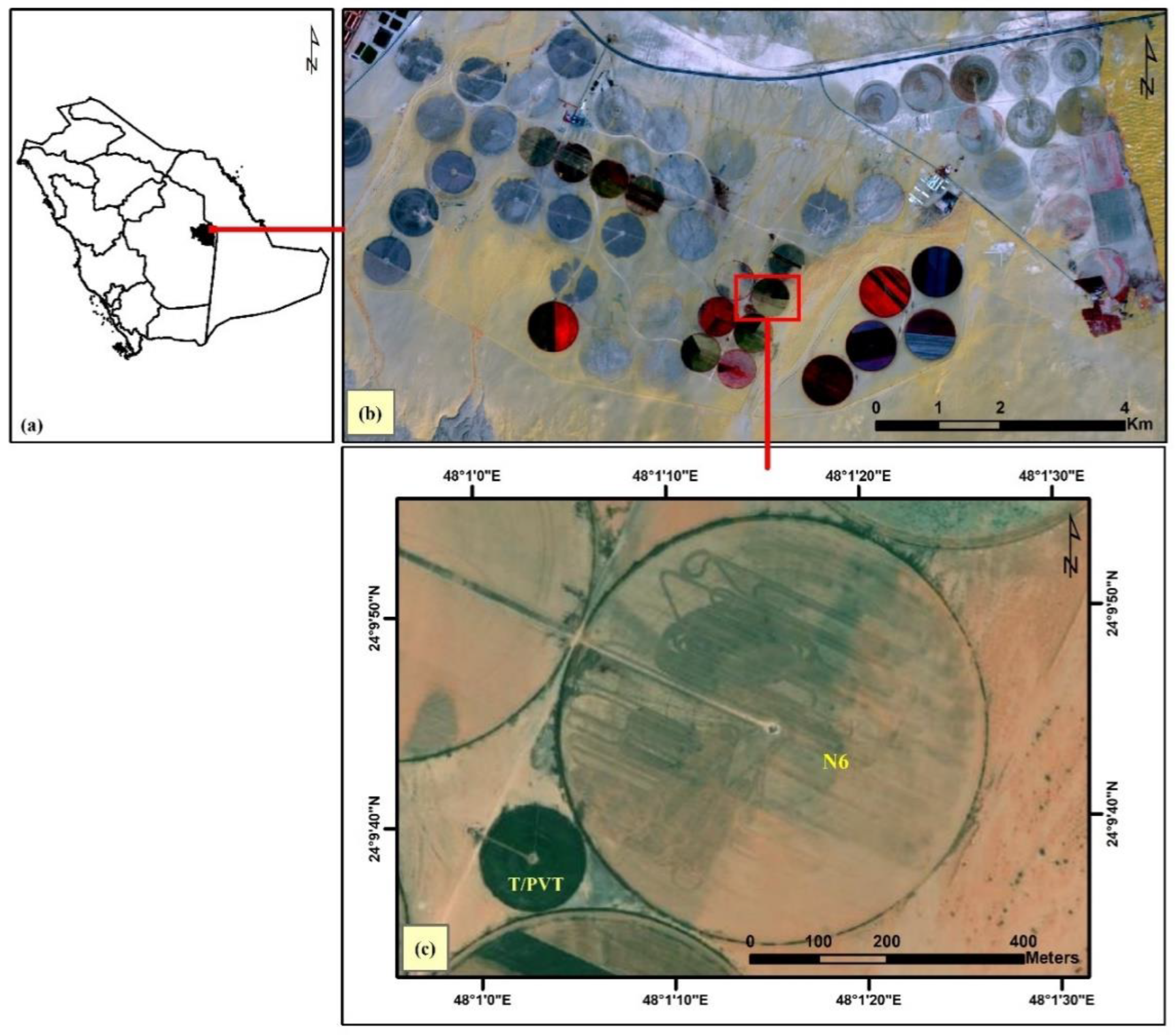
2.1. Experimental Area
2.2. Experimental Details
2.3. Field Sampling and Data Collection
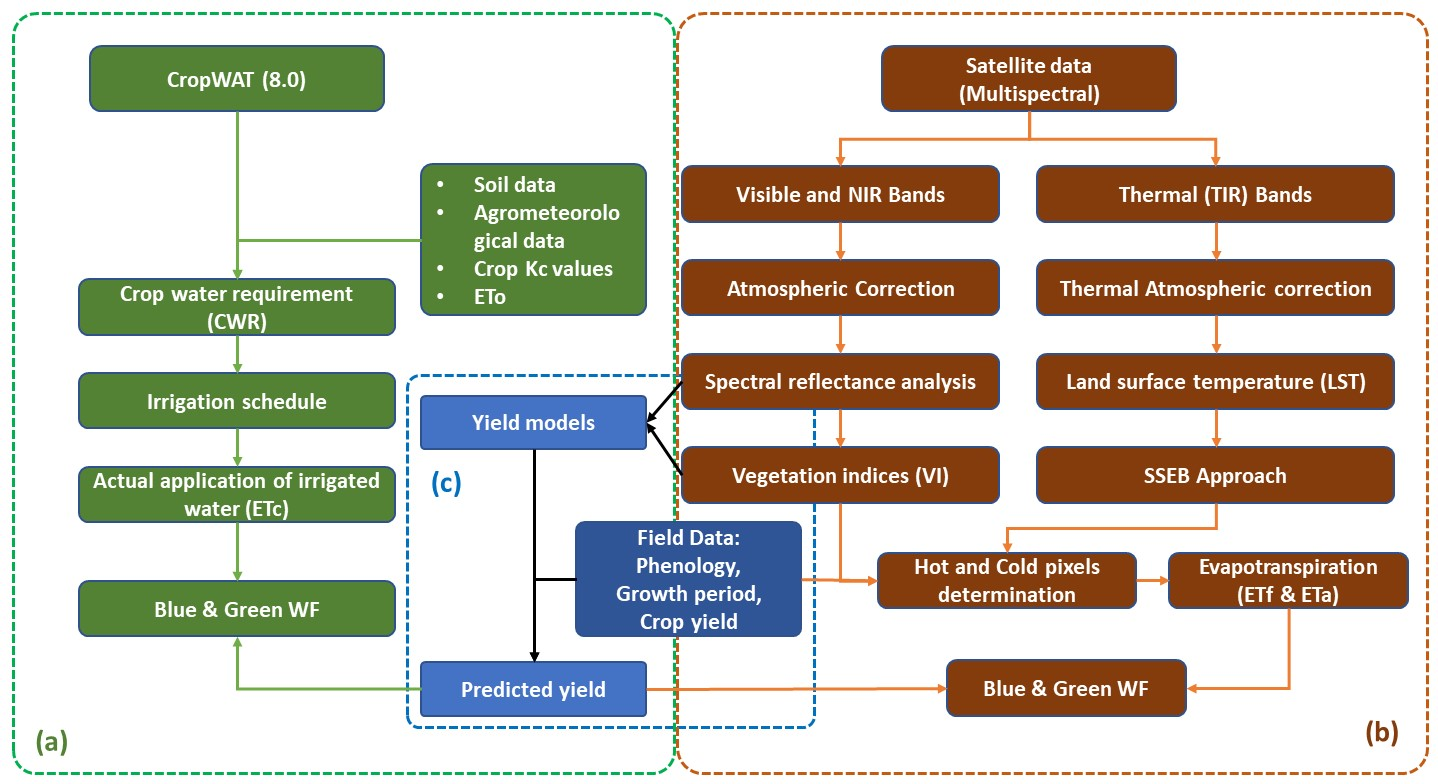
2.4. Water Footprint Assessment
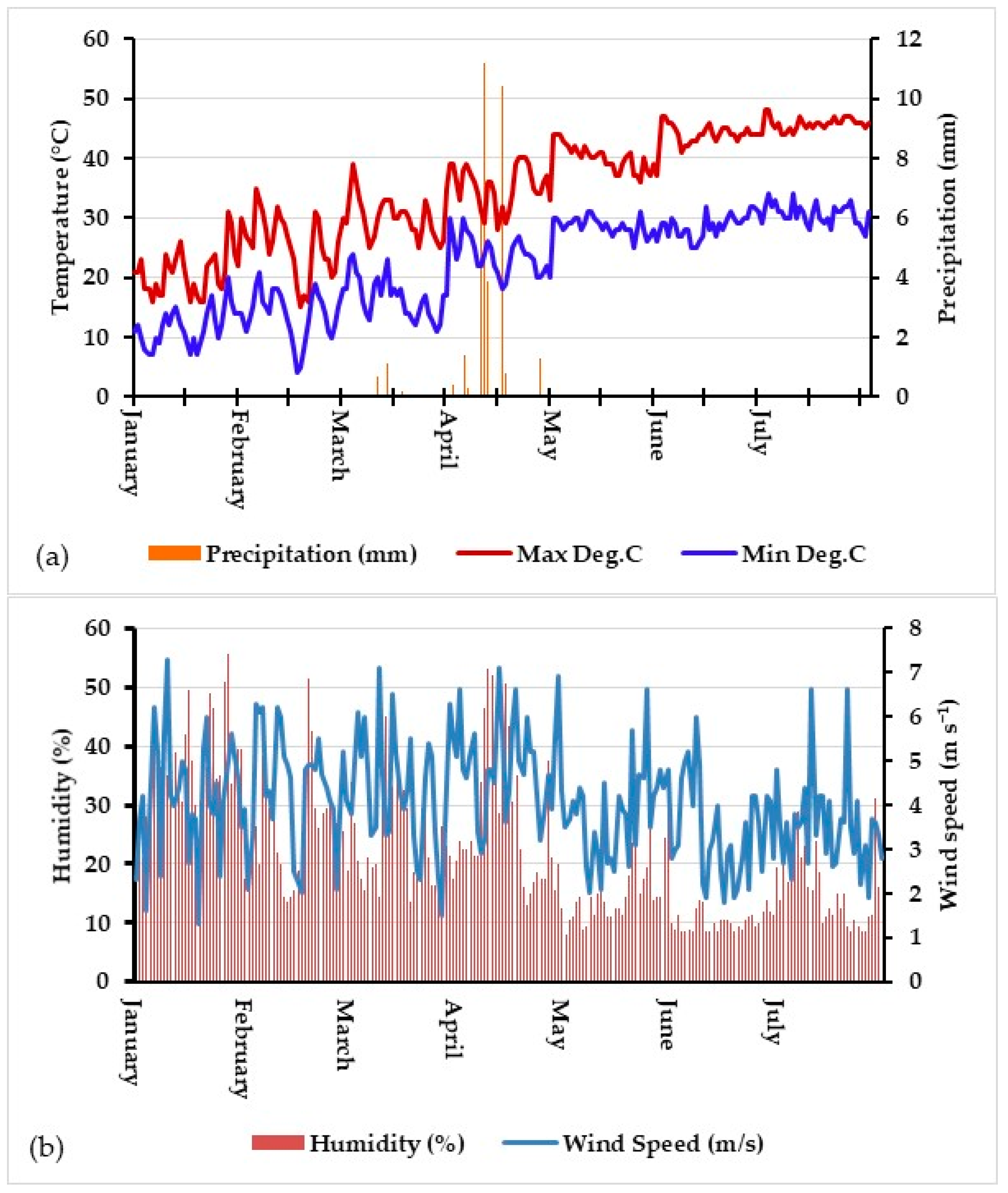
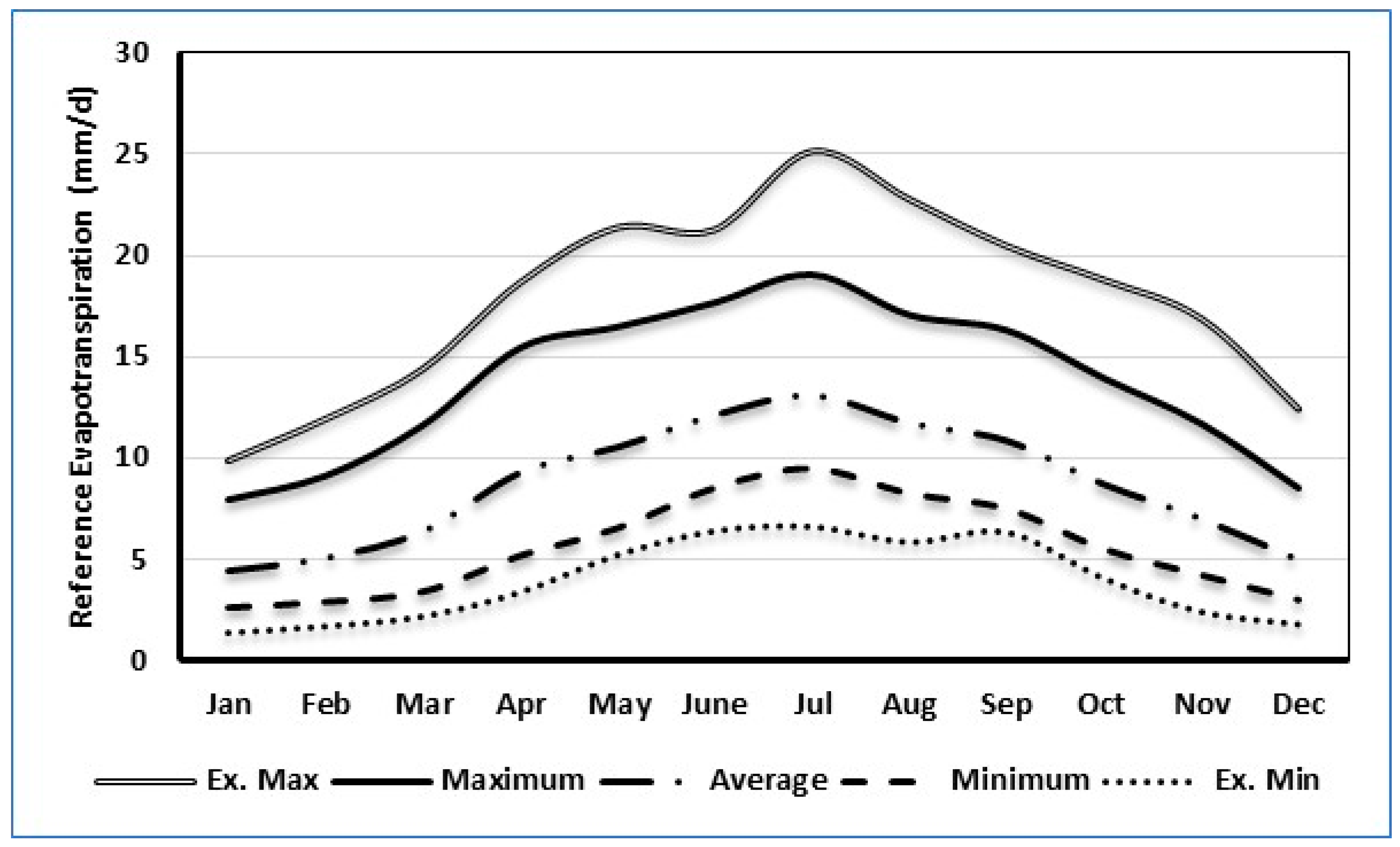
2.4.1. CROPWAT Input Data

| Parameter | Carrots | Onions | |
|---|---|---|---|
| Root depth (cm) | Min. | 18.00 | 15.00 |
| Max. | 35.00 | 25.00 | |
| Crop coefficients (length of the growth period in days) | Kc—initial | 0.35 (30) | 0.40 (15) |
| Kc—mid | 1.15 (50) | 1.05 (30) | |
| Kc—end | 0.65 (60) | 0.60 (15) | |
| Soil characteristics | Bulk density (g cm−3) | 1.27 | 1.29 |
| Field capacity | 0.34 | 0.34 | |
| Wilting point | 0.25 | 0.25 | |
2.4.2. Satellite Data and Image Analysis
2.5. Estimation of Crop Productivity
2.6. Estimation of the Crop Water Use
2.7. Assessment of Crop Water Footprint
2.8. Statistical Analysis
3. Results
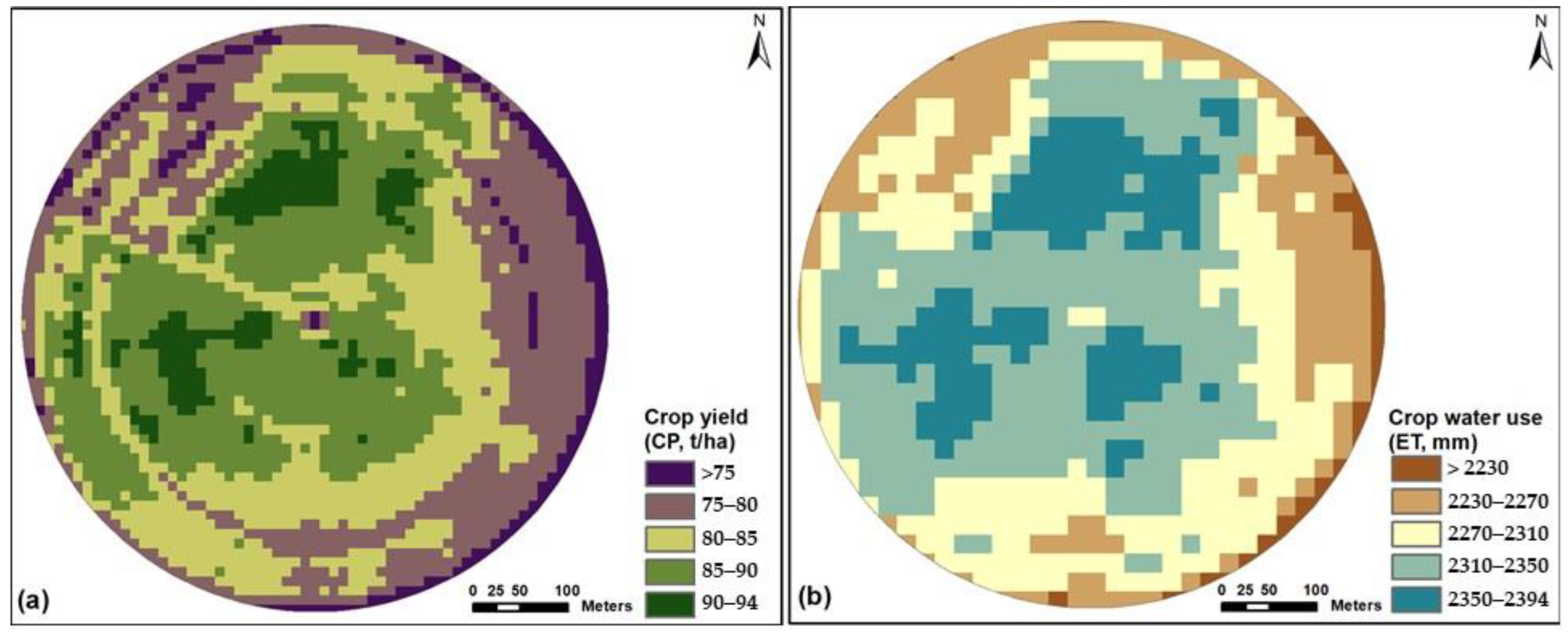
3.1. Crop Yields
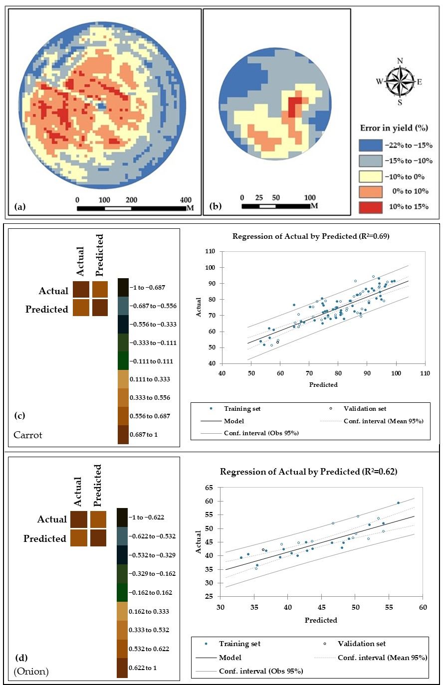
3.2. Yield Prediction Models
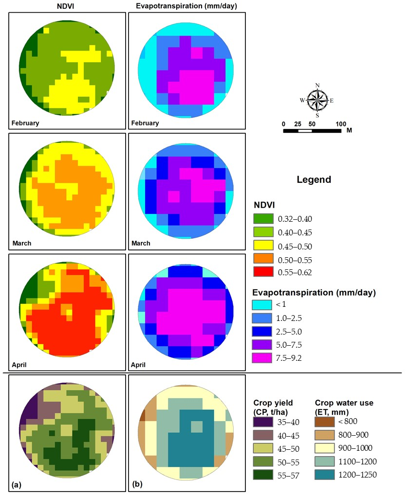
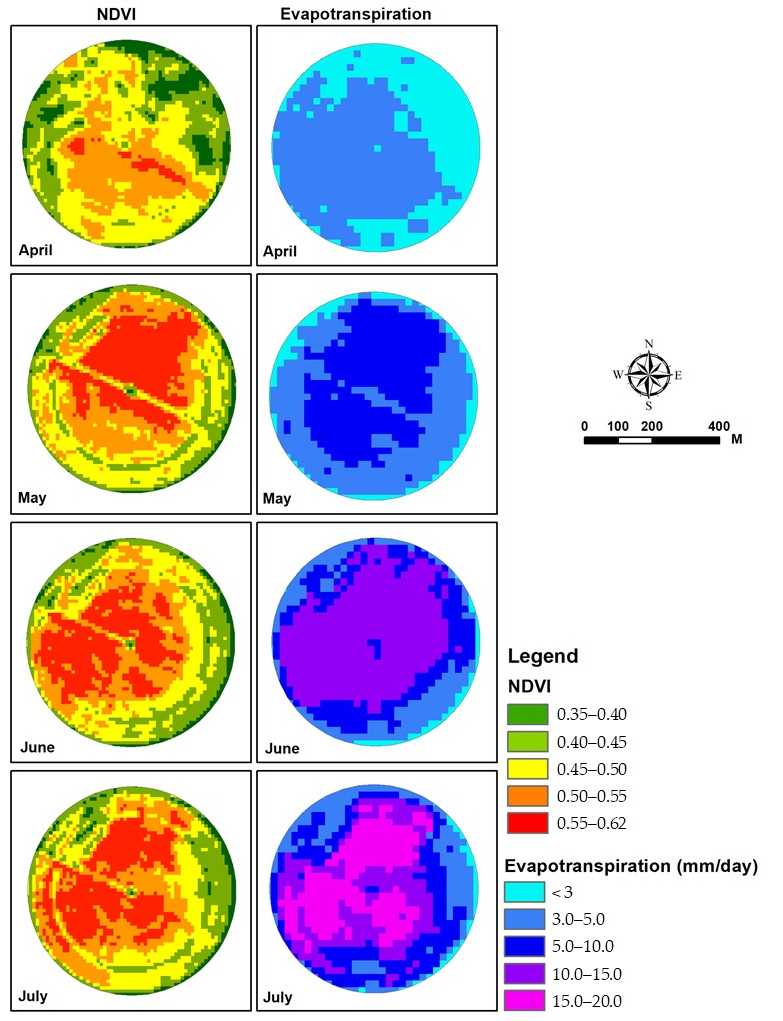
3.3. Evapotranspiration Mapping
4. Discussion
| Crop | Predicted Yield-YP (kg ha−1) | CWU (i.e., ETa, mm) | Water Footprint—WF (m3 t−1) | Reference | ||
|---|---|---|---|---|---|---|
| WFG | WFB | WFG+B | ||||
| Carrots | 74 | 2320 | 16 | 283 | 312 | This study |
| 23 | 427 | 450 | [34] | |||
| 106 | 28 | 134 | [36] | |||
| 104 | 12 | 116 | [37] | |||
| 0 | 114 | 114 | [38] | |||
| Onions | 44 | 1001 | 9 | 227 | 230 | This study |
| 18 | 243 | 261 | [34] | |||
| 176 | 53 | 229 | [35] | |||
| 192 | 88 | 280 | [36] | |||
5. Conclusions
Author Contributions
Funding
Data Availability Statement
Acknowledgments
Conflicts of Interest
Abbreviations
| Acronym/Variable | Explanation |
| CP | Crop productivity |
| CWU | Crop water use |
| CWUB | Crop water use—blue WF component |
| CWUG | Crop water use—green WF component |
| ET | Evapotranspiration |
| ETa | Actual evapotranspiration |
| ETc | Crop evapotranspiration |
| ETf | Evapotranspiration factor |
| ETo | Observed evapotranspiration |
| Kc | Crop coefficient |
| L8 | Landsat-8 |
| LST | Land surface temperature |
| S2 | Sentinel-2 |
| SSEB | Simplified surface energy balance |
| WF | Water footprint |
| WFG | Water footprint—green component |
| WFB | Water footprint—blue component |
| VIs | Vegetation indices |
References
- Xinchun, C.; Mengyang, W.; Rui, S.; La, Z.; Dan, C.; Guangcheng, S.; Shuhai, T. Water footprint assessment for crop production based on field measurements: A case study of irrigated paddy rice in East China. Sci. Total Environ. 2018, 610–611, 84–93. [Google Scholar] [CrossRef]
- Hoekstra, A.Y.; Hung, P.Q. Virtual water trade: A quantification of virtual water flows between nations in relation to international crop trade. In Value of Water Research Report Series 11; IHE: Delft, The Netherlands, 2002; Available online: https://www.waterfootprint.org/media/downloads/Report11.pdf (accessed on 26 August 2022).
- Hoekstra, A.Y.; Chapagain, A.K.; Mekonnen, M.M.; Aldaya, M.M. The Water Footprint Assessment Manual: Setting the Global Standard; Routledge: London, UK, 2011; p. 154. [Google Scholar]
- Hoekstra, A.Y. Virtual water: An introduction. In Virtual Water Trade: Proceedings of the International Expert Meeting on Virtual Water Trade; Value of Water Research Report Series 12; IHE: Delft, The Netherlands, 2003; Available online: https://www.waterfootprint.org/media/downloads/Report12.pdf (accessed on 26 August 2022).
- Mahmoud, S.H.; Gan, T.Y. Irrigation water management in arid regions of Middle East: Assessing spatio-temporal variation of actual evapotranspiration through remote sensing techniques and meteorological data. Agric. Water Manag. 2019, 212, 35–47. [Google Scholar] [CrossRef]
- Rodriguez, C.I.; Ruiz de Galarreta, V.A.; Kruse, E.E. Analysis of water footprint of potato production in the pampean region of Argentina. J. Clean. Prod. 2015, 90, 91–96. [Google Scholar] [CrossRef]
- Madugundu, R.; Al-Gaadi, K.A.; Tola, E.; Hassaballa, A.A.; Kayad, A.G. Utilization of Landsat-8 data for the estimation of carrot and maize crop water footprint under the arid climate of Saudi Arabia. PLoS ONE 2018, 13, e0192830. [Google Scholar] [CrossRef] [PubMed] [Green Version]
- Geng, Q.; Ren, Q.; Nolan, R.H.; Wu, P.; Yu, Q. Assessing China’s agricultural water use efficiency in a green-blue water perspective: A study based on data envelopment analysis. Ecol. Indic. 2019, 96, 329–335. [Google Scholar] [CrossRef]
- Gebremariam, F.T.; Habtu, S.; Yazew, E.; Teklu, B. The water footprint of irrigation-supplemented cotton and mung-bean crops in Northern Ethiopia. Heliyon 2021, 7, e06822. [Google Scholar] [CrossRef] [PubMed]
- Lambin, E.F.; Cashman, P.; Moody, A.; Parkhurst, B.H.; Pax, M.H.; Schaaf, C.B. Agricultural Production Monitoring in the Sahel Using Remote-Sensing—Present Possibilities and Research Needs. J. Environ. Manag. 1993, 38, 301–322. [Google Scholar] [CrossRef]
- Aldaya, M.M.; Llamas, M.R. Water Footprint analysis for the Guadiana river basin. In Value of Water Research Report Series No. 35; UNESCO-IHE Institute for Water Education: Delft, The Netherlands, 2008; Available online: http://waterfootprint.org/media/downloads/Report35-WaterFootprint-Guadiana_1.pdf (accessed on 26 March 2020).
- Tuninetti, M.; Tamea, S.; D’Odorico, P.; Laio, F.; Ridolfi, L. Global sensitivity of high-resolution estimates of crop water footprint. Water Resour. Res. 2015, 51, 8257–8272. [Google Scholar] [CrossRef] [Green Version]
- Senay, G.B.; Budde, M.E.; Verdin, J.P. Enhancing the Simplified Surface Energy Balance (SSEB) approach for estimating landscape ET: Validation with the METRIC model. Agric. Water Manag. 2011, 98, 606–618. [Google Scholar] [CrossRef]
- Senay, G.B.; Budde, M.; Verdin, J.P.; Melesse, A.M. A coupled remote sensing and simplified surface energy balance approach to estimate actual evapotranspiration from irrigated fields. Sensors 2007, 7, 979–1000. [Google Scholar] [CrossRef]
- McShane, R.R.; Driscoll, K.P.; Roy, S. A Review of Surface Energy Balance Models for Estimating Actual Evapotranspiration with Remote Sensing at High Spatiotemporal Resolution over Large Extents; U.S. Geological Survey Scientific Investigations Report; U.S. Geological Survey: Reston, VA, USA, 2017; 19p. [Google Scholar] [CrossRef] [Green Version]
- Chapagain, A.K.; Hoekstra, A.Y.; Savenije, H.H.G.; Gautam, R. The water footprint of cotton consumption: An assessment of the impact of worldwide consumption of cotton products on the water resources in the cotton producing countries. Ecol. Econ. 2006, 60, 186–203. [Google Scholar] [CrossRef]
- Aldaya, M.M.; Santos, P.M.; Llamas, M.R. Incorporating the water footprint and virtual water into policy: Reflections from the Mancha Occidental Region, Spain. Water Resour. Manag. 2010, 24, 941–958. [Google Scholar] [CrossRef] [Green Version]
- Tsakmakis, I.D.; Zoidou, M.; Gikas, G.D.; Sylaios, G.K. Impact of irrigation technologies and strategies on cotton water footprint using AquaCrop and CROPWAT models. Environ. Process. 2018, 5, 181–199. [Google Scholar] [CrossRef]
- Karandish, F.; Simunek, J. A comparison of the HYDRUS (2D/3D) and SALTMED models to investigate the influence of various water-saving irrigation strategies on the maize water footprint. Agric. Water Manag. 2019, 213, 809–820. [Google Scholar] [CrossRef] [Green Version]
- Zhuo, L.; Mekonnen, M.; Hoekstra, A.Y. Sensitivity and uncertainty in crop water footprint accounting: A case study for the Yellow River basin. Hydrol. Earth Syst. Sci. 2014, 18, 2219–2234. [Google Scholar] [CrossRef] [Green Version]
- Lovarelli, D.; Bacenetti, J.; Fiala, M. Water Footprint of crop productions: A review. Sci. Total Environ. 2016, 548–549, 236–251. [Google Scholar] [CrossRef]
- Allen, R.G.; Pereira, S.L.; Raes, D.; Smith, M. Crop Evapotranspiration. Guidelines for Computing Crop Water Requirement FAO Irrigation and Drainage Paper 56; FAO: Rome, Italy, 1998; Available online: http://www.fao.org/docrep/X0490E/X0490E00.htm (accessed on 9 December 2021).
- Doorenbos, J.; Pruitt, W.O. Crop Water Requirements. FAO Irrigation and Drainage Paper No. 24; Food and Agriculture Organization of the U.N.: Rome, Italy, 1977. [Google Scholar]
- Bastiaanssen, W.G.M.; Menenti, M.; Feddes, R.A.; Holtslag, A.A.M. A remote sensing surface energy balance algorithm for land (SEBAL): 1. Formulation. J. Hydrol. 1998, 212, 213–229. [Google Scholar] [CrossRef]
- Allen, R.G.; Tasumi, M.; Morse, A.; Trezza, R. A Landsat-based energy balance and evapotranspiration model in Western US water rights regulation and planning. Irrig. Drain. Syst. 2005, 19, 251–268. [Google Scholar] [CrossRef]
- Scarpare, F.V.; Hernandes, T.A.D.; Ruiz-Correa, S.T.; Picoli, M.C.A.; Scanlon, B.R.; Chagas, M.F.; Cardoso, T.d.F. Sugarcane land use and water resources assessment in the expansion area in Brazil. J. Clean. Prod. 2016, 133, 1318–1327. [Google Scholar] [CrossRef]
- Borsato, E.; Martello, M.; Marinello, F.; Bortolini, L. Environmental and economic sustainability assessment for two different sprinkler and A drip irrigation systems: A case study on maize cropping. Agriculture 2019, 9, 187. [Google Scholar] [CrossRef] [Green Version]
- Thompson, R. Some factors affecting carrot root shape and size. Euphytica 1969, 18, 277–285. [Google Scholar] [CrossRef]
- Sri Agung, I.G.A.M.; Blair, G.J. Effects of soil bulk density and water regime on carrot yield harvested at different growth stages. J. Hortic. Sci. Biotechnol. 1989, 64, 17–25. [Google Scholar] [CrossRef]
- Dawuda, M.M.; Boateng, P.Y.; Hemeng, O.B.; Nyarko, G. Growth and yield response of carrot (Daucus carota L.) to different rates of soil amendments and spacing. J. Sci. Technol. 2011, 31, 11–22. [Google Scholar] [CrossRef] [Green Version]
- Bezerra, B.G.; da Silva, B.B.; dos Santos, C.A.C.; Bezerra, J.R.C. Actual Evapotranspiration Estimation Using Remote Sensing: Comparison of SEBAL and SSEB Approaches. Adv. Remote Sens. 2015, 4, 234–247. [Google Scholar] [CrossRef] [Green Version]
- Saggi, M.; Jain, S. Reference evapotranspiration estimation and modeling of the Punjab Northern India using deep learning. Comput. Electron. Agric. 2018, 156, 387–398. [Google Scholar] [CrossRef]
- Granata, F. Evapotranspiration evaluation models based on machine learning algorithms—A comparative study. Agric. Water Manag. 2019, 217, 303–315. [Google Scholar] [CrossRef]
- Multsch, S.; Al-Rumaikhani, Y.; Frede, H.; Breuer, L. A site-specific agricultural water requirement and footprint estimator (SPARE: WATER 1.0). Geosci. Model Dev. 2013, 6, 1043–1059. [Google Scholar] [CrossRef]
- Penaloza-Sanchez, A.M.; Bustamante-Gonzalez, A.; Vargas-Lopez, S.; Quevedo-Nolasco, A. Water footprint of onion (Alliumcepa L.) and husk tomato (Physalis ixocarpa Brot.) crops in the region of Atlixco, Puebla, Mexico. Technol. Cienc. Agua 2020, 11, 1–30. [Google Scholar] [CrossRef]
- Mekonnen, M.; Hoekstra, A. The green, blue and grey water footprint of crops and derived crop products. Hydrol. Earth Syst. Sci. 2011, 15, 1577–1600. [Google Scholar] [CrossRef]
- Roux, B.L.; Van der Laan, M.; Vahrmeijer, T.; Annandale, J.G.; Bristow, K.L. Estimating Water Footprints of Vegetable Crops: Influence of Growing Season, Solar Radiation Data and Functional Unit. Water 2016, 8, 473. [Google Scholar] [CrossRef]
- Matlala, M.N. Estimation of the Volumetric Water Footprint of Carrot (Daucus carota L.) and Swiss Chard (Beta Vulgaris L.) Grown in Gauteng Province, South Africa. Master’s Thesis, Department of Plant and Soil Sciences, University of Pretoria, Hatfield, Pretoria, South Africa, 2019; p. 40. [Google Scholar]


| Satellite | Particulars | Source |
|---|---|---|
| Sentinel-2 | Level 2A (MSI) BOA | https://scihub.copernicus.eu (accessed on 30 May 2022) |
| Landsat-8 | Level 2A (OLI, TIRS) | https://earthexplorer.usgs.gov (accessed on 28 August 2022) |
| Weather data | Historical monthly weather data (2000–2020 *) | https://Worldclim.org (accessed on 12 September 2022) |
| Crop | Yield (t ha−1) | NDVI | Mean | ||
|---|---|---|---|---|---|
| 0.18–0.35 | 0.35–0.50 | 0.50–0.62 | |||
| Carrots | Total yield | 61.85 | 74.90 | 85.61 | 74.12 |
| Commercial yield | 47.22 | 54.64 | 67.21 | 56.36 | |
| Aboveground biomass | 13.30 | 15.47 | 17.34 | 15.37 | |
| Onions | Total yield | 36.54 | 44.75 | 51.63 | 44.31 |
| Commercial yield | 30.93 | 36.05 | 44.16 | 37.05 | |
| Aboveground biomass | 3.84 | 5.22 | 5.81 | 4.96 | |
| Crop | Model No. | Prediction Model | Model | Cross-Validation | ||
|---|---|---|---|---|---|---|
| R2 | R2 | MBE (%) | RMSE (%) | |||
| Carrots | M1 | 1143.6 × NIR 2212 459.51 | 0.77 ** | 0.64 ** | 7.82 | 13.41 |
| M2 | 973.1 × EVI − 226.51 | 0.69 ** | 0.62 ** | –17.46 | 9.21 | |
| M3 | 962.86 × RDVI − 219.74 | 0.58 ** | 0.59 ** | 5.98 | 10.43 | |
| Onions | M1 | 915.78 × NIR − 316.2 | 0.68 * | 0.61 * | –17.19 | 12.65 |
| M2 | 1756.4 × RDVI − 360.81 | 0.72 ** | 0.69 ** | 15.21 | 17.67 | |
| M3 | 1314.3 × EVI − 253.29 | 0.52 ** | 0.49 ** | –6.19 | 11.24 | |
| Month | Carrots | Onions | ||||
|---|---|---|---|---|---|---|
| ETa | RMSE (%) | MBE (%) | ETa | RMSE (%) | MBE (%) | |
| February | 272 | −3.63 | −13.2 | |||
| March | 234.0 | −1.97 | −3.9 | 351 | −2.76 | −7.6 |
| April | 391.6 | 7.82 | 61.1 | 378 | −3.33 | −11.1 |
| May | 560.2 | −0.77 | −0.6 | |||
| June | 522.0 | −6.06 | −36.7 | |||
| July | 612.1 | −4.67 | −21.8 | |||
| Overall | 2319.9 | −1.13 | −12.6 | 1001 | −3.24 | −9.0 |
| Reference Data | ||||||||
|---|---|---|---|---|---|---|---|---|
| ETo | ETa (Onions) | AWA (Onions) | ETa (Carrots) | AWA (Carrots) | SUM | User’s Accuracy | ||
| Map data | ETo | 18 | 1 | 2 | 0 | 0 | 21 | 85.71% |
| ETa (onions) | 3 | 19 | 1 | 2 | 1 | 26 | 73.07% | |
| AWA (onions) | 0 | 5 | 17 | 4 | 1 | 27 | 62.96% | |
| ETc (carrots) | 4 | 2 | 1 | 19 | 6 | 32 | 59.37% | |
| AWA (carrots) | 1 | 1 | 2 | 2 | 23 | 29 | 79.31% | |
| SUM | 26 | 28 | 23 | 27 | 31 | 135 | 72.08% | |
| Producer’s accuracy | 69.23% | 67.85% | 73.91% | 70.37% | 74.19% | 71.11% | ||
| Overall accuracy | (18 + 19 + 17 + 19 + 23)/135 = 71.11% | |||||||
Publisher’s Note: MDPI stays neutral with regard to jurisdictional claims in published maps and institutional affiliations. |
© 2022 by the authors. Licensee MDPI, Basel, Switzerland. This article is an open access article distributed under the terms and conditions of the Creative Commons Attribution (CC BY) license (https://creativecommons.org/licenses/by/4.0/).
Share and Cite
Al-Gaadi, K.A.; Madugundu, R.; Tola, E.; El-Hendawy, S.; Marey, S. Satellite-Based Determination of the Water Footprint of Carrots and Onions Grown in the Arid Climate of Saudi Arabia. Remote Sens. 2022, 14, 5962. https://doi.org/10.3390/rs14235962
Al-Gaadi KA, Madugundu R, Tola E, El-Hendawy S, Marey S. Satellite-Based Determination of the Water Footprint of Carrots and Onions Grown in the Arid Climate of Saudi Arabia. Remote Sensing. 2022; 14(23):5962. https://doi.org/10.3390/rs14235962
Chicago/Turabian StyleAl-Gaadi, Khalid A., Rangaswamy Madugundu, ElKamil Tola, Salah El-Hendawy, and Samy Marey. 2022. "Satellite-Based Determination of the Water Footprint of Carrots and Onions Grown in the Arid Climate of Saudi Arabia" Remote Sensing 14, no. 23: 5962. https://doi.org/10.3390/rs14235962