
A Method for Forest Canopy Height Inversion Based on Machine Learning and Feature Mining Using UAVSAR


Abstract
:1. Introduction
2. Materials and Methods
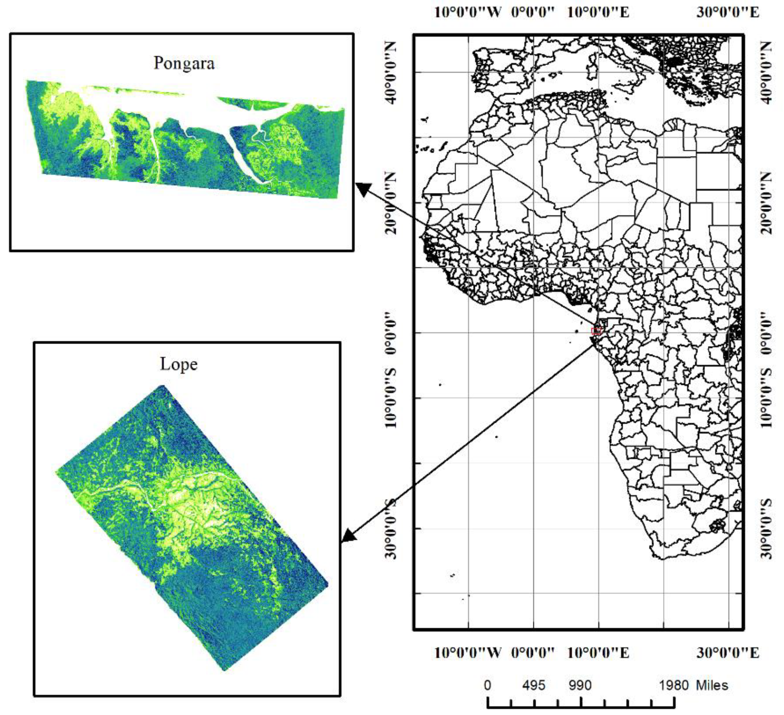
2.1. Study Area and Data
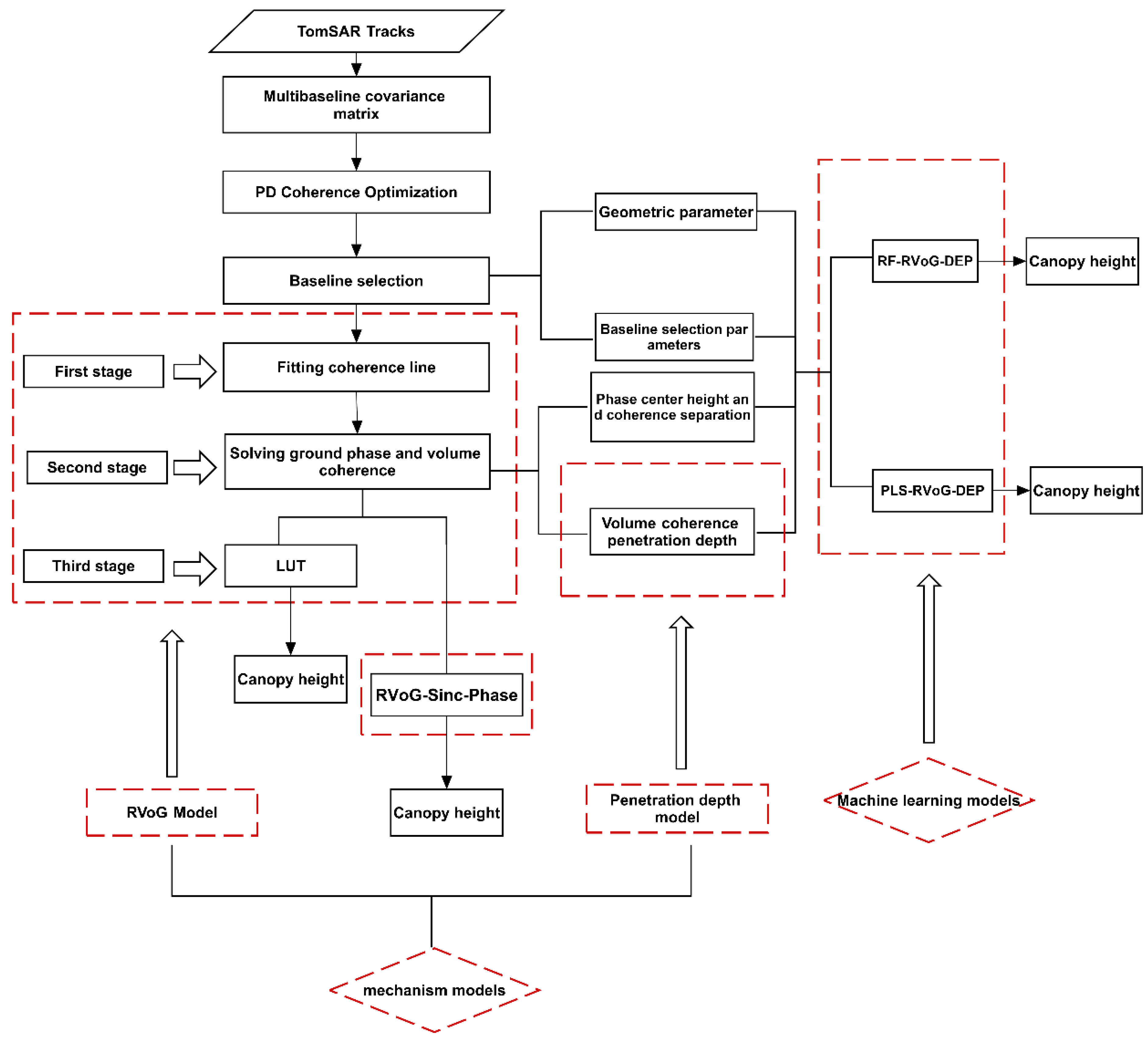
2.2. Methods
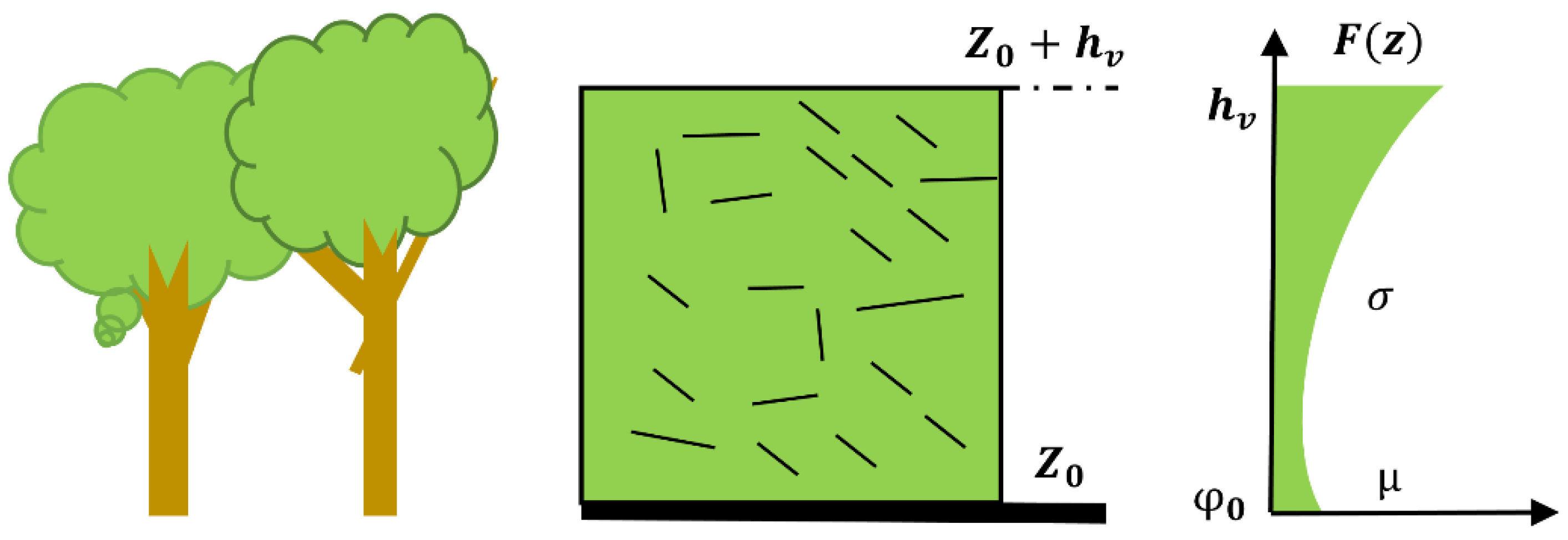
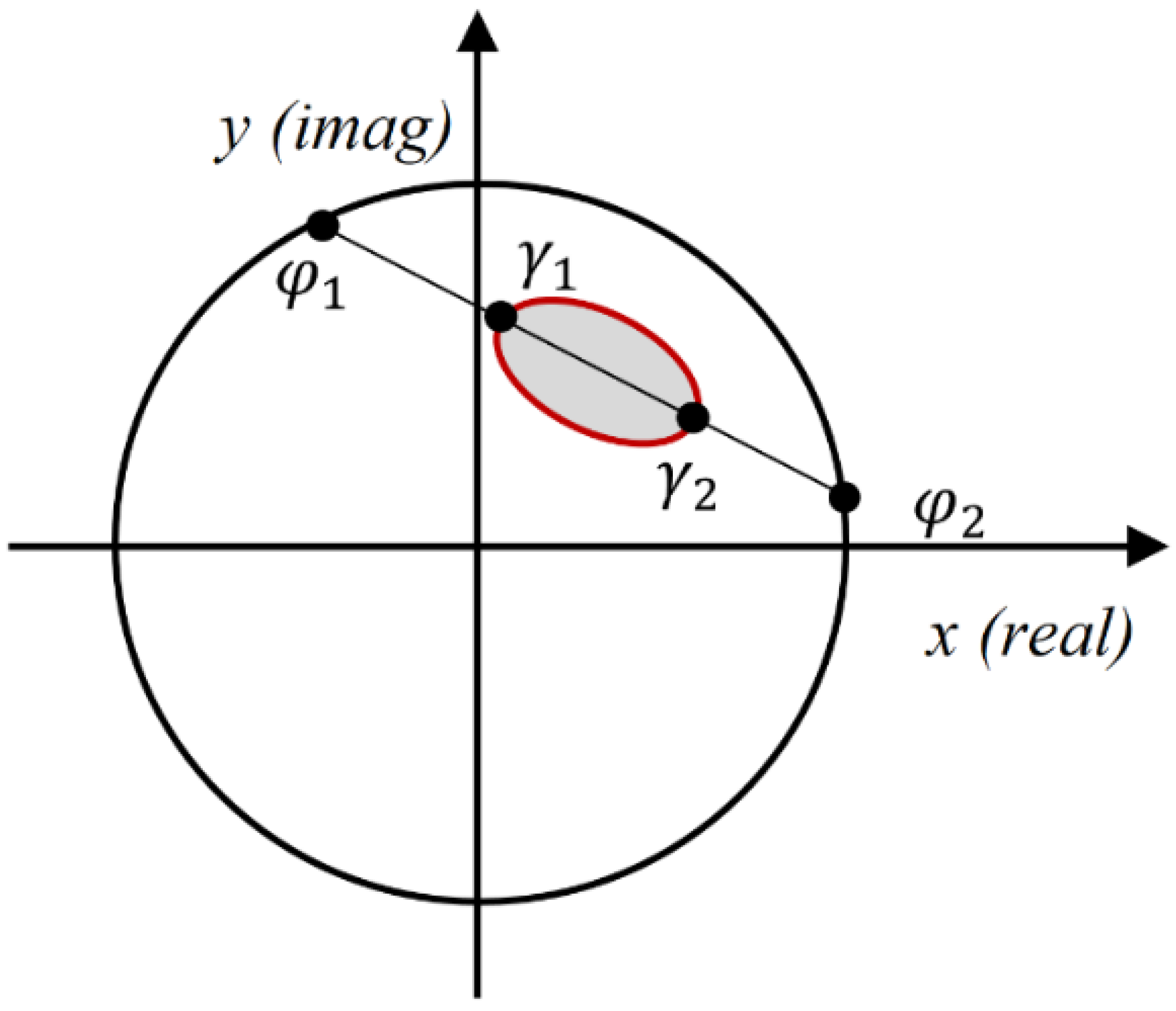
2.2.1. Mechanism Model
- (1)
- RVoG model
- (2)
- Phase-coherence amplitude combined inversion method
- (3)
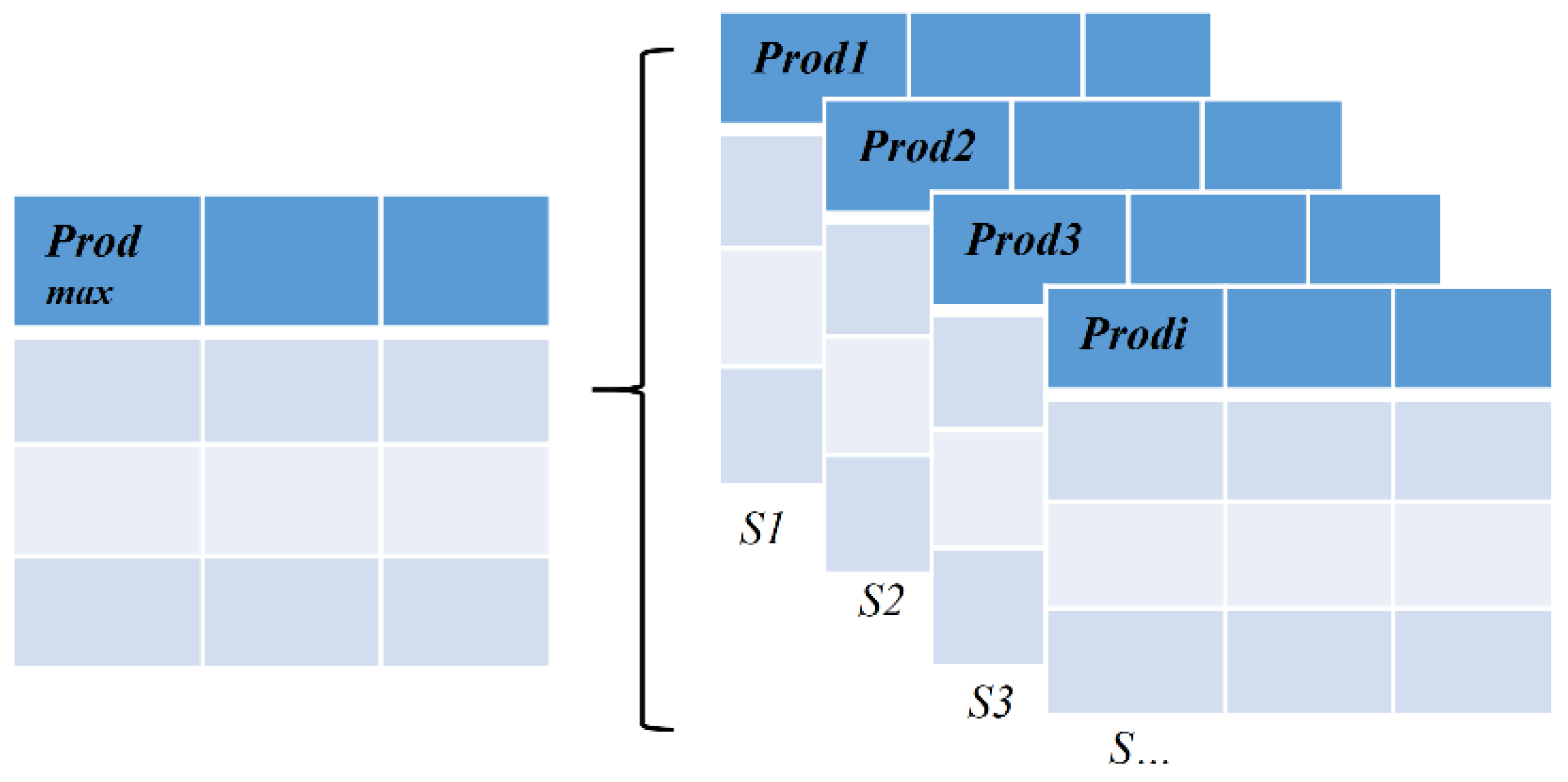
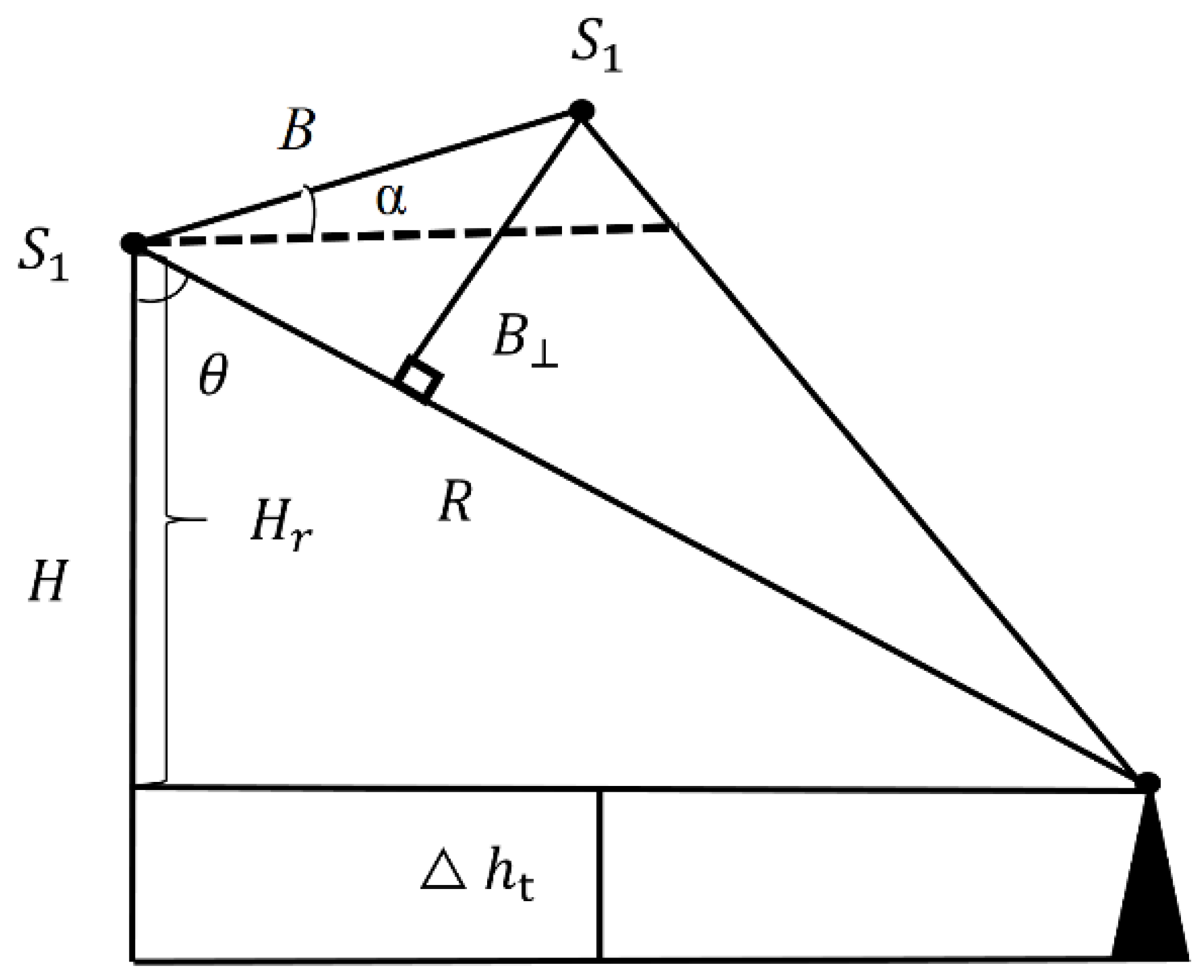
- Baseline selection method

- (4)
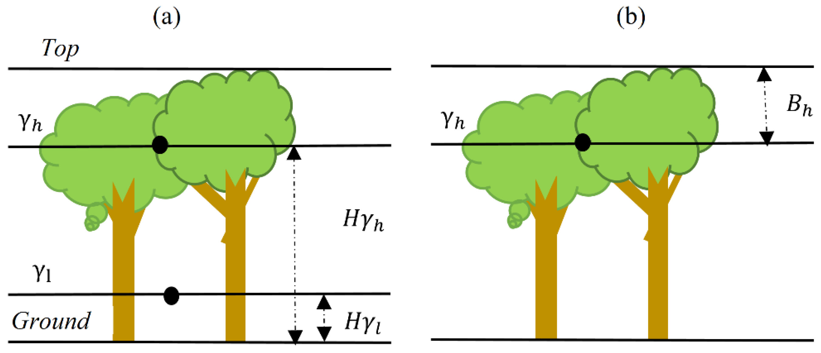
- Penetration depth model
2.2.2. Machine Learning Methods
- (1)
- Independent variable extraction
- (a)
- Vertical height parameter
- (b)
- Baseline selection parameters
- (c)
- Geometric parameters
- (2)
- Regression Model Development
- (a)
- Partial least squares regression model
Y = [y] n × 1
- (b)
- Random forest regression model
3. Results
3.1. Mechanism Model Inversion Results
3.2. Machine Learning Method Inversion Results
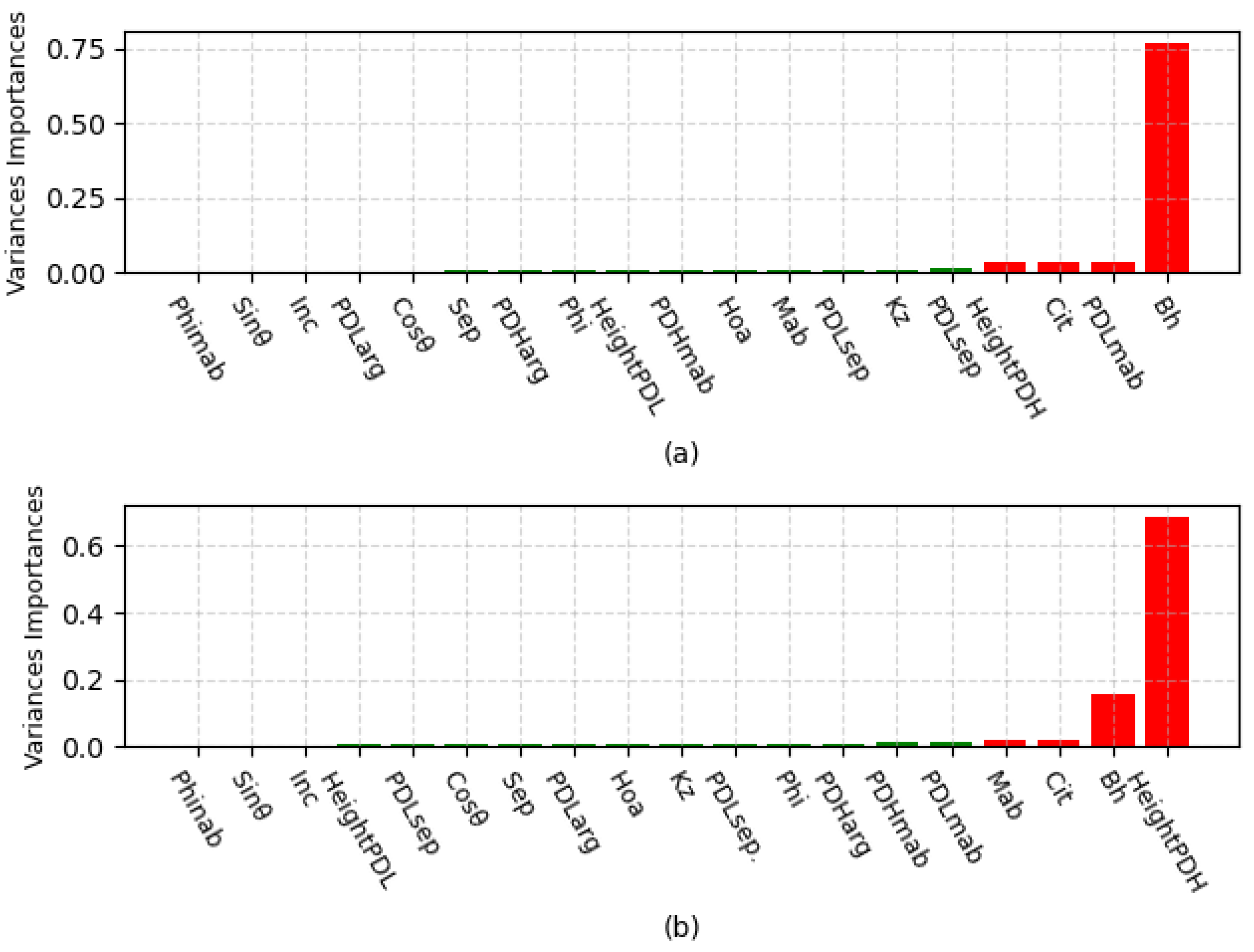
3.2.1. Importance Analysis of Independent Variables
3.2.2. Inversion Results
4. Discussion
4.1. Limitations of the Mechanism Model
4.2. The Effect of Temporal De-Correlation
4.3. Effect of Baseline Selection Method and Observation Geometry
4.4. Uncertainty of Machine Learning Methods
5. Conclusions
Author Contributions
Funding
Data Availability Statement
Acknowledgments
Conflicts of Interest
References
- Goetz, S.; Dubayah, R. Advances in remote sensing technology and implications for measuring and monitoring forest carbon stocks and change. Carbon Manag. 2011, 2, 231–244. [Google Scholar] [CrossRef]
- Zhao, P.; Lu, D.; Wang, G.; Wu, C.; Huang, Y.; Yu, S. Examining Spectral Reflectance Saturation in Landsat Imagery and Corresponding Solutions to Improve Forest Aboveground Biomass Estimation. Remote Sens. 2016, 8, 469. [Google Scholar] [CrossRef] [Green Version]
- Hall, F.G.; Bergen, K.; Blair, J.B.; Dubayah, R.; Houghton, R.; Hurtt, G.; Kellndorfer, J.; Lefsky, M.; Ranson, J.; Saatchi, S.; et al. Characterizing 3D vegetation structure from space: Mission requirements. Remote Sens. Environ. 2011, 115, 2753–2775. [Google Scholar] [CrossRef] [Green Version]
- Xu, M.; Xiang, H.; Yun, H.; Ni, X.; Chen, W.; Cao, C.-X. Retrieval of forest canopy height jointly using airborne LiDAR and ALOS PALSAR data. J. Appl. Remote Sens. 2019, 14, 022203. [Google Scholar] [CrossRef]
- Bao, Y.; Cao, C.; Chen, W.; Tian, R.; Dang, Y.; Li, L.; Li, G. Extraction of forest structural parameters based on the intensity information of high-density airborne light detection and ranging. J. Appl. Remote Sens. 2012, 6, 063533. [Google Scholar] [CrossRef] [Green Version]
- Zhang, L.; Duan, B.; Zou, B. Research on Inversion Models for Forest Height Estimation Using Polarimetric Sar Interferometry. ISPRS-Int. Arch. Photogramm. Remote Sens. Spat. Inf. Sci. 2017, 42, 659–663. [Google Scholar] [CrossRef] [Green Version]
- Graham, L.C. Synthetic Interferometer Radar For Topographic Mapping. Proc. IEEE. 1974, 62, 763–768. [Google Scholar] [CrossRef]
- Garestier, F.; Le Toan, T. Forest Modeling For Height Inversion Using Single-Baseline InSAR/Pol-InSAR Data. IEEE Trans. Geosci. Remote Sens. 2010, 48, 1528–1539. [Google Scholar] [CrossRef]
- Soja, M.J.; Ulander, L.M.H. Digital canopy model estimation from TanDEM-X interferometry using high-resolution lidar DEM. In Proceedings of the 2013 IEEE International Geoscience and Remote Sensing Symposium-IGARSS, Melbourne, Australia, 21–26 July 2013. [Google Scholar]
- Sadeghi, Y.; St-Onge, B.; Leblon, B.; Simard, M.; Papathanassiou, K. Mapping forest canopy height using TanDEM-X DSM and airborne LiDAR DTM. In Proceedings of the 2014 IEEE Geoscience and Remote Sensing Symposium, Quebec City, QC, Canada, 13–18 July 2014. [Google Scholar]
- Treuhaft, R.N.; Moghaddam, M.; van Zyl, J.J. Vegetation Characteristics And Underlying Topography Frominterferometer Radar. Radio Sci. 1996, 31, 1449–1485. [Google Scholar] [CrossRef]
- Cloude, S.R.; Papathanassiou, K.P. Three-Stage Inversion Process For Polarimetric SAR Interferometry. IEE Proc.-Radar. Sonar. Navig. 2003, 150, 125–134. [Google Scholar] [CrossRef]
- Papathanassiou, K.; Cloude, S.R. Single-baseline polarimetric SAR interferometry. IEEE Trans. Geosci. Remote Sens. 2001, 39, 2352–2363. [Google Scholar] [CrossRef] [Green Version]
- Hajnsek, I.; Kugler, F.; Lee, S.K. Tropical-forest-parameter estimation by means of Pol-InSAR: The INDREX-II campaign. IEEE Trans. Geosci. Remote Sens. 2009, 47, 481–493. [Google Scholar] [CrossRef] [Green Version]
- Liao, Z.; He, B.; Quan, X.; van Dijk, A.I.; Qiu, S.; Yin, C. Biomass estimation in dense tropical forest using multiple information from single-baseline P-band PolInSAR data. Remote Sens. Environ. 2018, 221, 489–507. [Google Scholar] [CrossRef]
- Cloude, S.R.; Papathanassiou, K.P. Forest vertical structure estimation using coherence tomography. In Proceedings of the IEEE International Geoscience and Remote Sensing Symposium IGARSS, Boston, MA, USA, 7–11 July 2008. [Google Scholar]
- Zahriban Hesari, M.; Shataee, S.; Maghsoudi, Y.; Mohammadi, J.; Fransson, J.E.; Persson, H.J. Forest Variable Estimations Using TanDEM-X Data in Hyrcanian Forests. Can. J. Remote Sens. 2020, 46, 166–176. [Google Scholar] [CrossRef]
- Persson, H.J.; Fransson, J.E.S. Comparison between TanDEM-X-and ALS-based estimation of aboveground biomass and tree height in boreal forests. Scand. J. For. Res. 2017, 32, 306–319. [Google Scholar] [CrossRef] [Green Version]
- Brigot, G.; Simard, M.; Colin-Koeniguer, E.; Boulch, A. Retrieval of Forest Vertical Structure from PolInSAR Data by Machine Learning Using LIDAR-Derived Features. Remote Sens. 2019, 11, 381. [Google Scholar] [CrossRef] [Green Version]
- Fore, A.G.; Chapman, B.D.; Hawkins, B.P.; Hensley, S.; Jones, C.E.; Michel, T.R.; Muellerschoen, R.J. UAVSAR Polarimetric Calibration. IEEE Trans. Geosci. Remote Sens. 2015, 53, 3481–3491. [Google Scholar] [CrossRef]
- Armston, J.; Tang, H.; Hancock, S.; Marselis, S.; Duncanson, L.; Kellner, J.; Hofton, M.; Blair, J.B.; Fatoyinbo, T.; Dubayah, R.O. AfriSAR: Gridded Forest Biomass and Canopy Metrics Derived from LVIS, Gabon, 2016; ORNL DAAC: Oak Ridge, TN, USA, 2020. [Google Scholar]
- Xie, Q.H.; Wang, C.C.; Zhu, J.J.; Fu, H.Q. Forest height inversion by combining S-RVOG model with terrain factor and PD coherence optimization. Acta Geod. Cartogr. Sin. 2015, 44, 686–693. [Google Scholar]
- Kugler, F.; Lee, S.K.; Hajnsek, I.; Papathanassiou, K.P. Forest Height Estimation by Means of Pol-InSAR Data Inversion: The Role of the Vertical Wavenumber. IEEE Trans. Geosci. Remote Sens. 2015, 53, 5294–5311. [Google Scholar] [CrossRef]
- Denbina, M.; Simard, M. Kapok: An open source Python library for PolInSAR forest height estimation using UA VSAR data. In Proceedings of the 2017 IEEE International Geoscience and Remote Sensing Symposium (IGARSS), Fort Worth, TX, USA, 23–28 July 2017. [Google Scholar]
- Lee, S.K.; Kugler, F.; Papathanassiou, K.; Hajnsek, I. Multibaseline polarimetric SAR interferometry forest height inversion approaches. In Proceedings of the ESA POLinSAR Workshop, Frascati, Italy, 24–28 January 2011. [Google Scholar]
- Denbina, M.; Simard, M.; Hawkins, B. Forest Height Estimation Using Multibaseline PolInSAR and Sparse Lidar Data Fusion. IEEE J. Sel. Top. Appl. Earth Obs. Remote Sens. 2018, 11, 3415–3433. [Google Scholar] [CrossRef]
- Luo, H.B.; Zhu, B.D.; Yue, C.R.; Wang, N. Forest Canopy Height Inversion Based On Airborne Multi-Baseline PolInSAR. J. Geomatics. 2022, 48, 1–7. [Google Scholar]
- Dall, J. InSAR Elevation Bias Caused by Penetration Into Uniform Volumes. IEEE Trans. Geosci. Remote Sens. 2007, 45, 2319–2324. [Google Scholar] [CrossRef]
- Schlund, M.; Baron, D.; Magdon, P.; Erasmi, S. Canopy penetration depth estimation with TanDEM-X and its compensation in temperate forests. ISPRS J. Photogramm. Remote Sens. 2019, 147, 232–241. [Google Scholar] [CrossRef]
- Kong, X.; Cao, Z.; An, Q.; Gao, Y.; Du, B. Quality-Related and Process-Related Fault Monitoring With Online Monitoring Dynamic Concurrent PLS. IEEE Access 2018, 6, 59074–59086. [Google Scholar] [CrossRef]
- Hoeppner, J.M.; Skidmore, A.K.; Darvishzadeh, R.; Heurich, M.; Chang, H.C.; Gara, T.W. Mapping canopy chlorophyll content in a temperate forest using airborne hyperspectral data. Remote Sens. 2020, 12, 3573. [Google Scholar] [CrossRef]
- Ali, A.M.; Darvishzadeh, R.; Skidmore, A.; Gara, T.W.; O’Connor, B.; Roeoesli, C.; Heurich, M.; Paganini, M. Comparing methods for mapping canopy chlorophyll content in a mixed mountain forest using Sentinel-2 data. Int. J. Appl. Earth Obs. Geoinf. 2020, 87, 102037. [Google Scholar] [CrossRef]
- Breiman, L. Random Forests. Mach. Learn. 2001, 45, 5–32. [Google Scholar] [CrossRef] [Green Version]
- Purohit, S.; Aggarwal, S.P.; Patel, N.R. Estimation of forest aboveground biomass using combination of Landsat 8 and Sentinel-1A data with random forest regression algorithm in Himalayan Foothills. Trop. Ecol. 2021, 62, 288–300. [Google Scholar] [CrossRef]
- Huang, H.; Liu, C.; Wang, X. Constructing a Finer-Resolution Forest Height in China Using ICESat/GLAS, Landsat and ALOS PALSAR Data and Height Patterns of Natural Forests and Plantations. Remote Sens. 2019, 11, 1740. [Google Scholar] [CrossRef] [Green Version]
- Lee, S.K.; Kugler, F.; Hajnsek, I.; Papathanassiou, K. The impact of temporal decorrelation over forest terrain in polarimetric SAR interferometry. In Proceedings of the International Workshop on Applications of Polarimetry and Polarimetric Interferometry (Pol-InSAR), Frascati, Italy, 26–30 January 2009. [Google Scholar]
- Lee, S.-K.; Kugler, F.; Papathanassiou, K.; Hajnsek, I. Quantification and compensation of temporal decorrelation effects in polarimetric SAR interferometry. In Proceedings of the 2012 IEEE International Geoscience and Remote Sensing Symposium, Munich, Germany, 22–27 July 2012. [Google Scholar]
- Zhou, Y.-S.; Hong, W.; Cao, F.; Wang, Y.-P.; Wu, Y.-R. Analysis of Temporal Decorrelation in Dual-Baseline Polinsar Vegetation Parameter Estimation. In Proceedings of the IEEE International Geoscience and Remote Sensing Symposium, Boston, MA, USA, 7–11 July 2008. [Google Scholar]
- Mette, T.; Kugler, F.; Papathanassiou, K.; Hajnsek, I. Forest and the random volume over ground-nature and effect of 3 possible error types. In Proceedings of the European Conference on Synthetic Aperture Radar (EUSAR), Dresden, Germany, 16–18 May 2006. [Google Scholar]
- Simard, M.; Denbina, M. An Assessment of Temporal Decorrelation Compensation Methods for Forest Canopy Height Estimation Using Airborne L-Band Same-Day Repeat-Pass Polarimetric SAR Interferometry. IEEE J. Sel. Top. Appl. Earth Obs. Remote Sens. 2018, 11, 95–111. [Google Scholar] [CrossRef]
- Lee, S.-K.; Kugler, F.; Papathanassiou, K.P.; Hajnsek, I. Quantifying temporal decorrelation over boreal forest at L-and P-band. In Proceedings of the 7th European Conference on Synthetic Aperture Radar, Friedrichshafen, Germany, 2–5 June 2008. [Google Scholar]
- Du, K.; Lin, H.; Wang, G.; Long, J.; Li, J.; Liu, Z. The Impact of Vertical Wavenumber on Forest Height Inversion by PolInSAR. In Proceedings of the 2018 Fifth International Workshop on Earth Observation and Remote Sensing Applications (EORSA), Xi’an, China, 18–20 June 2018. [Google Scholar]
- Chen, H.; Cloude, S.R.; Goodenough, D.G.; Hill, D.A.; Nesdoly, A. Radar Forest Height Estimation in Mountainous Terrain Using Tandem-X Coherence Data. IEEE J. Sel. Top. Appl. Earth Obs. Remote Sens. 2018, 11, 3443–3452. [Google Scholar] [CrossRef]


| Test Area | Number of Tracks | Vertical Baseline (m) | Range Resolution (m) | Azimuth Resolution (m) |
|---|---|---|---|---|
| Lope | 8 | 0, 20, 45, 105 | 3.33 | 4.8 |
| Pongara | 5 | 0, 20, 40, 60, 80, 100, 120 | 3.33 | 4.8 |
| Variable Type | Name | Description | Expressions |
|---|---|---|---|
| Coherence phase center height and coherence separation | PDHsep | High coherence separation | |
| PDLsep | Low coherence separation | ||
| PDHmab | High coherence magnitude | ||
| PDLmab | Low coherence amplitude | ||
| PDHarg | High coherence phases | ||
| PDLarg | Low coherence phases | ||
| Phi | Ground phase | / | |
| Phimab | Surface coherence amplitude | ||
| HeightPDH | High coherence phase center height | ||
| HeightPDL | Low coherence phase center height | ||
| Penetration depth | Bh | Penetration depth |
| Variable Type | Name | Description | Expressions |
|---|---|---|---|
| Baseline selection parameters | sep | Coherence separation | |
| mab | Coherence amplitude | ||
| cit | Product of coherence separation and coherence amplitude |
| Variable Type | Name | Description | Expressions |
|---|---|---|---|
| Geometric parameters | Cosθ | Incident angle cosine | None |
| Sinθ | Incident angle sine | None | |
| Inc | incident angle | None | |
| Kz | Vertical wave number | ||
| Hoa | Height of ambiguity |
| Test Area | N | Model | R2 | RMSE (m) | BIAS (m) |
|---|---|---|---|---|---|
| Lope | 4239 | RF-RVoG-DEP | 0.967 | 2.959 | −0.022 |
| PLS-RVoG-DEP | 0.847 | 6.380 | −0.012 | ||
| Pongara | 3068 | RF-RVoG-DEP | 0.979 | 2.226 | 0.013 |
| PLS-RVoG-DEP | 0.853 | 5.861 | −0.014 |
| Test Area | N | Model | R2 | RMSE (m) | BIAS (m) | |
|---|---|---|---|---|---|---|
| Lope | 2118 | Fusion Model | RF-RVoG-DEP | 0.900 | 5.154 | −0.061 |
| PLS-RVoG-DEP | 0.850 | 6.320 | 0.002 | |||
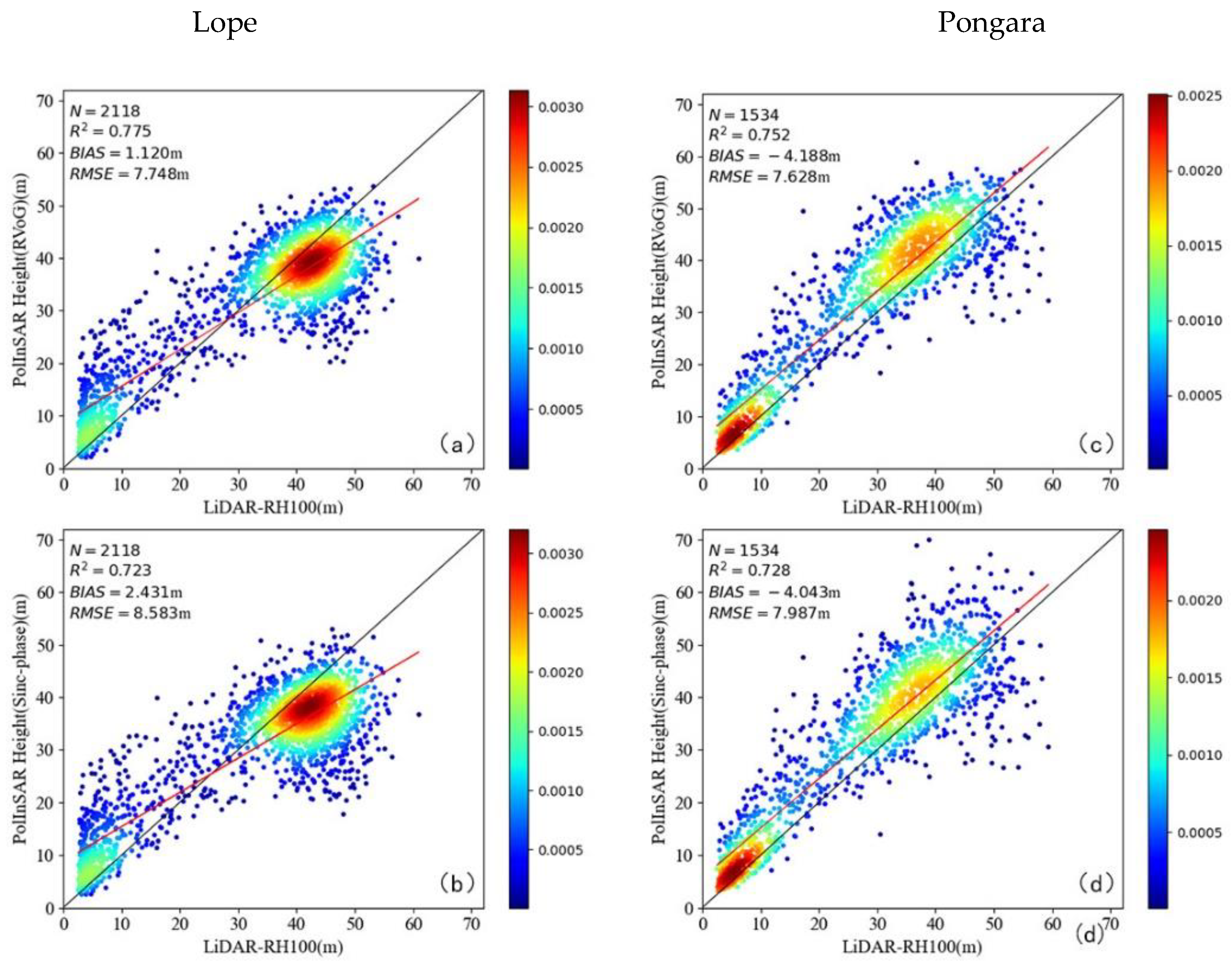
| Mechanism Model | RVoG | 0.775 | 7.748 | 1.120 | ||
| RVoG-Sinc-Phase | 0.723 | 8.583 | 2.431 | |||
| Pongara | 1534 | Fusion Model | RF-RVoG-DEP | 0.903 | 4.769 | 0.016 |
| PLS-RVoG-DEP | 0.869 | 5.534 | 0.038 | |||
| Mechanism Model | RVoG | 0.752 | 7.628 | −4.188 | ||
| RVoG-Sinc-Phase | 0.728 | 7.987 | −4.043 | |||
Publisher’s Note: MDPI stays neutral with regard to jurisdictional claims in published maps and institutional affiliations. |
© 2022 by the authors. Licensee MDPI, Basel, Switzerland. This article is an open access article distributed under the terms and conditions of the Creative Commons Attribution (CC BY) license (https://creativecommons.org/licenses/by/4.0/).
Share and Cite
Luo, H.; Yue, C.; Xie, F.; Zhu, B.; Chen, S. A Method for Forest Canopy Height Inversion Based on Machine Learning and Feature Mining Using UAVSAR. Remote Sens. 2022, 14, 5849. https://doi.org/10.3390/rs14225849
Luo H, Yue C, Xie F, Zhu B, Chen S. A Method for Forest Canopy Height Inversion Based on Machine Learning and Feature Mining Using UAVSAR. Remote Sensing. 2022; 14(22):5849. https://doi.org/10.3390/rs14225849
Chicago/Turabian StyleLuo, Hongbin, Cairong Yue, Fuming Xie, Bodong Zhu, and Si Chen. 2022. "A Method for Forest Canopy Height Inversion Based on Machine Learning and Feature Mining Using UAVSAR" Remote Sensing 14, no. 22: 5849. https://doi.org/10.3390/rs14225849