
Data-Driven Short-Term Daily Operational Sea Ice Regional Forecasting
 , , , , , ,
Abstract
:
1. Introduction
- 1.
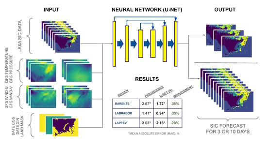
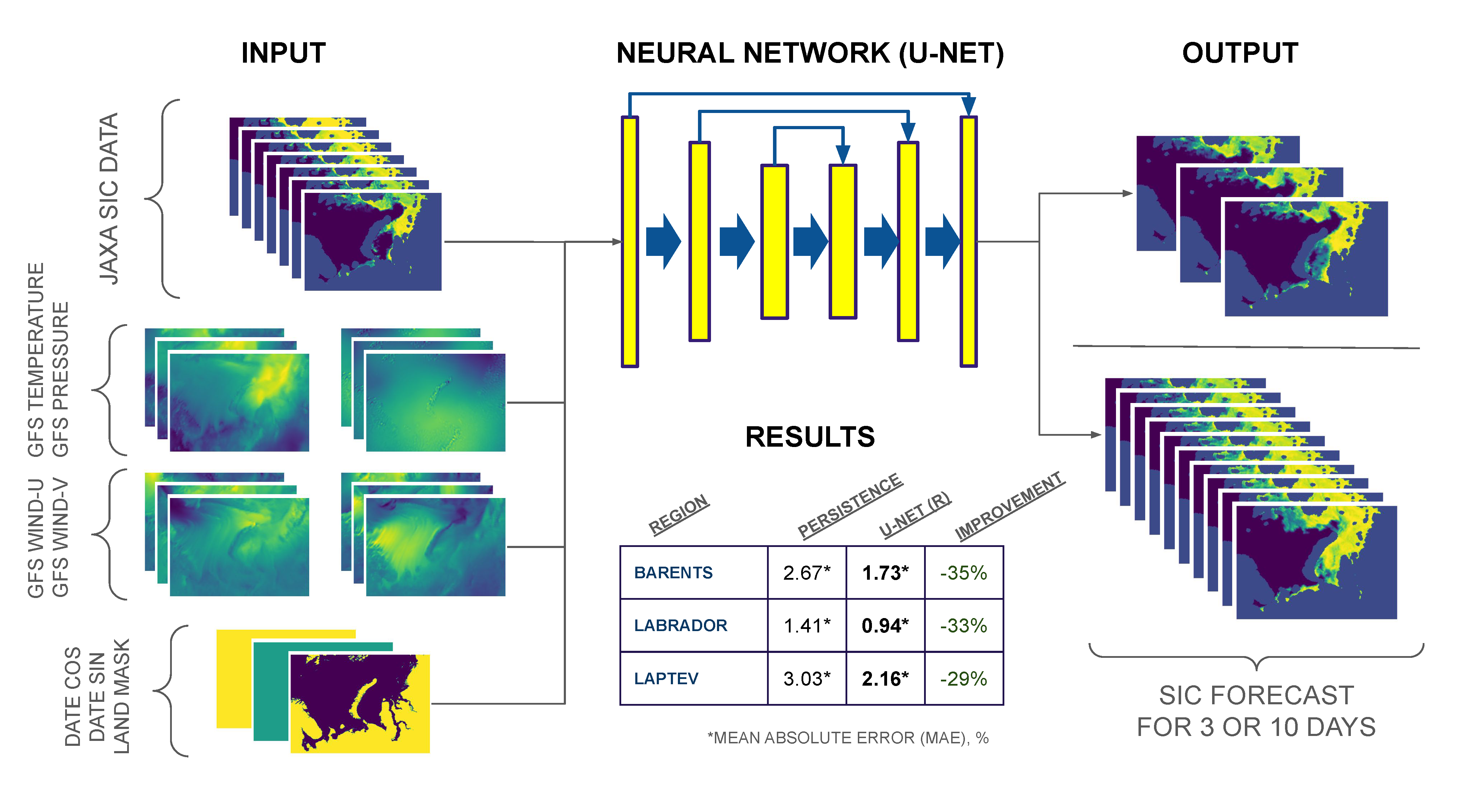
- We collect JAXA AMSR-2 Level-3 SIC data and GFS analysis and forecasts data, process it, and construct three regional datasets, which can be used as benchmark tasks for future research.
- 2.
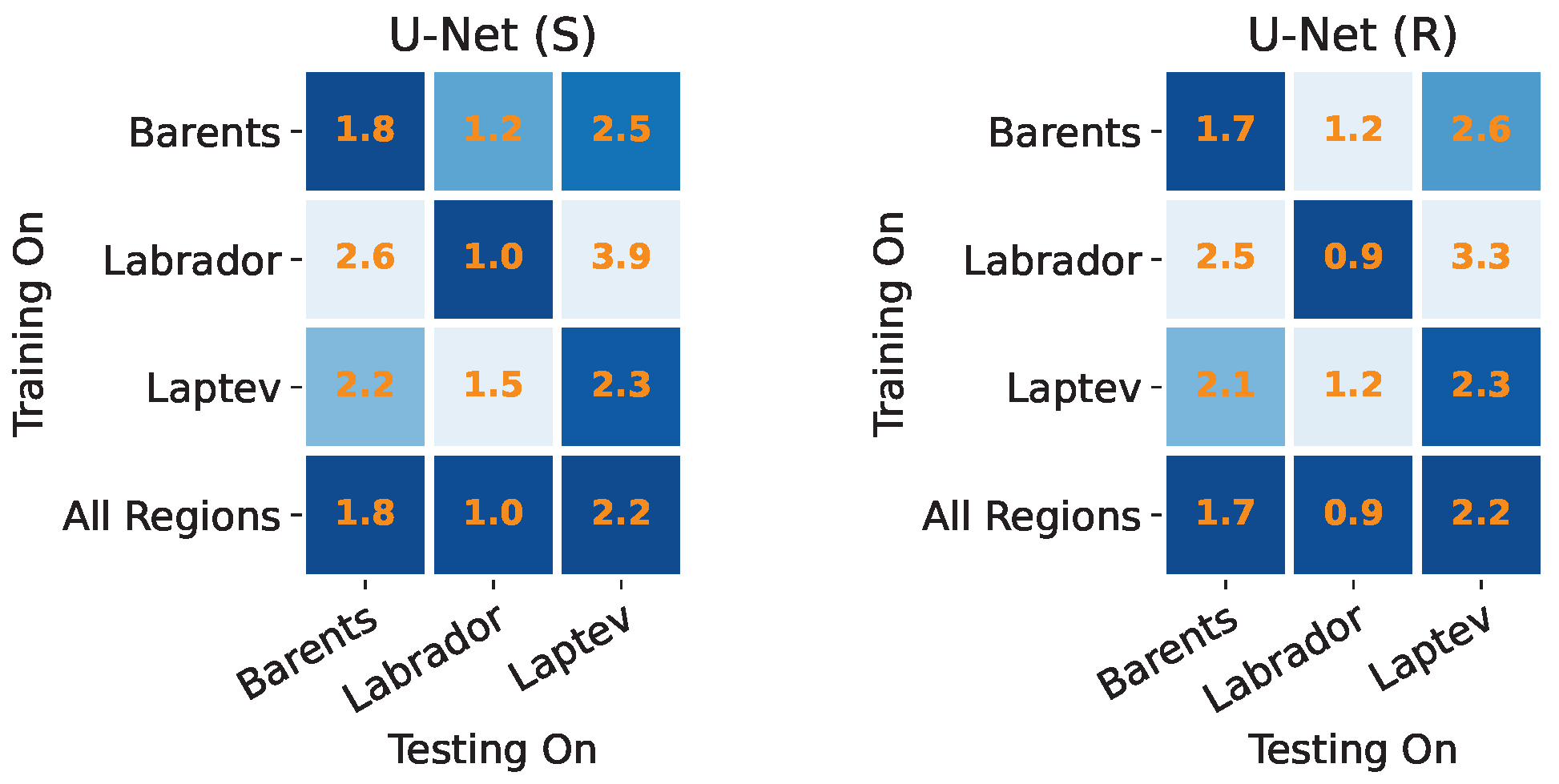
- We conduct numerous experiments on forecasting SIC maps with the U-Net model in two regimes and provide our findings on the prospect of this approach, including comparison with standard baselines, standard metric values, and model generalization ability.
- 3.
- We build a fast and reliable tool—trained on all three regions of the U-Net network that can provide operational sea ice forecasts in these Arctic regions.
- 4.
- We compare U-Net performance in forecasting in recurrent (R) and straightforward (S) regimes and highlight the strength and weaknesses of both.
2. Data
2.1. Sea Ice Data (JAXA AMSR-2 Level-3)
2.2. Weather Data (GFS)
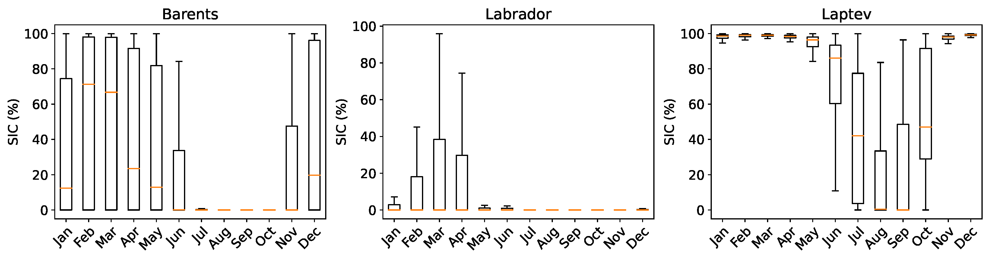
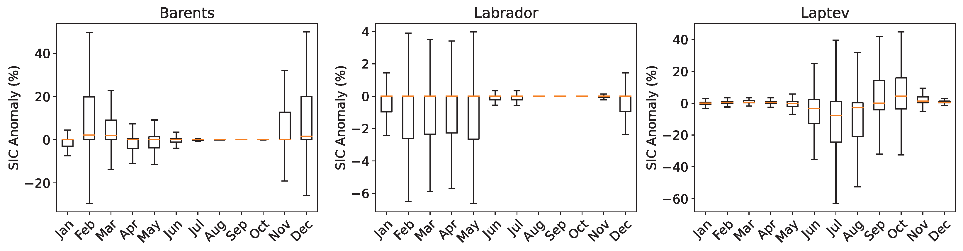
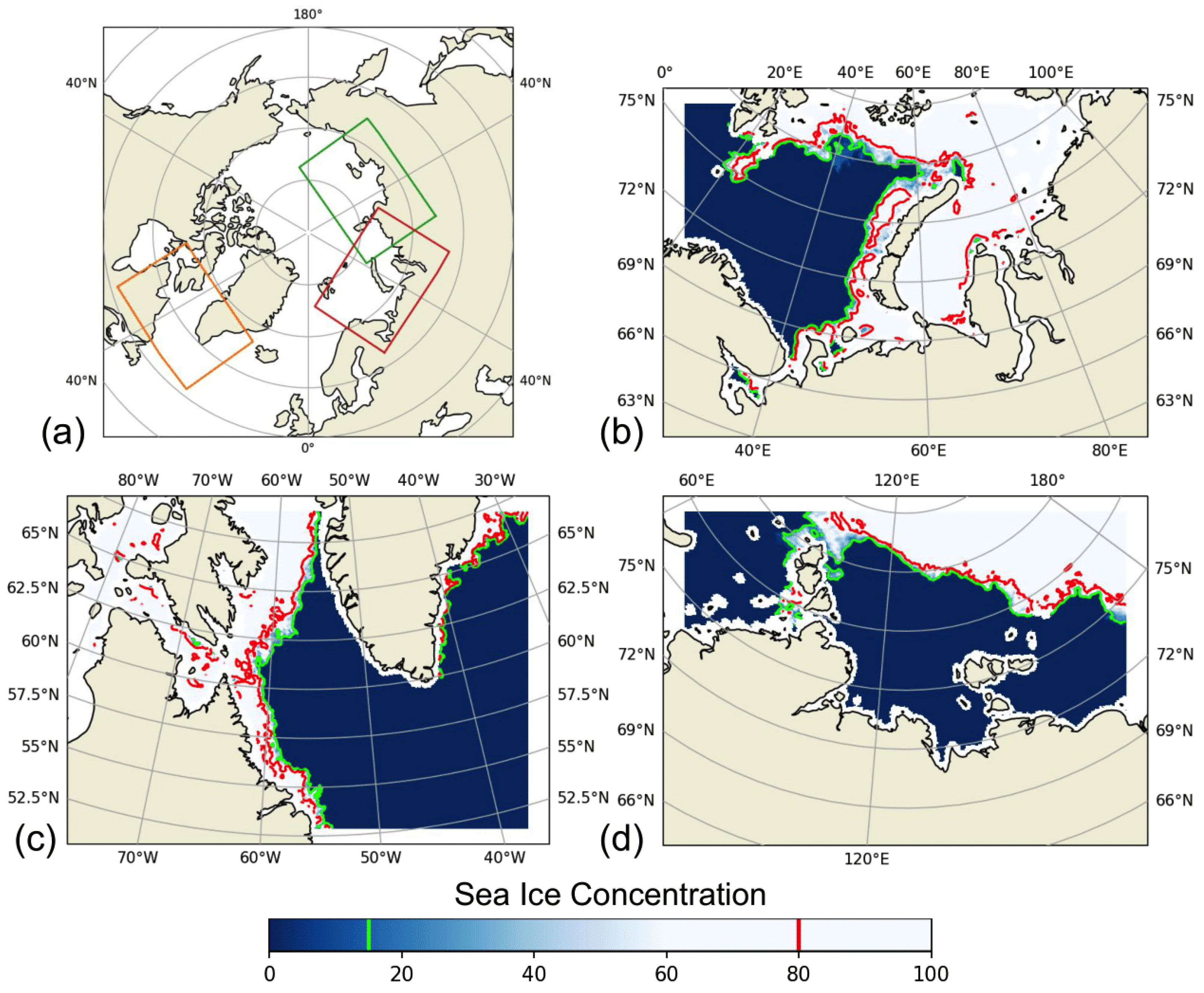
2.3. Regions
3. Methods
3.1. Data Split
3.2. Data Preprocessing
3.3. Baselines
3.4. Models
3.5. Metrics and Losses
3.6. Augmentations
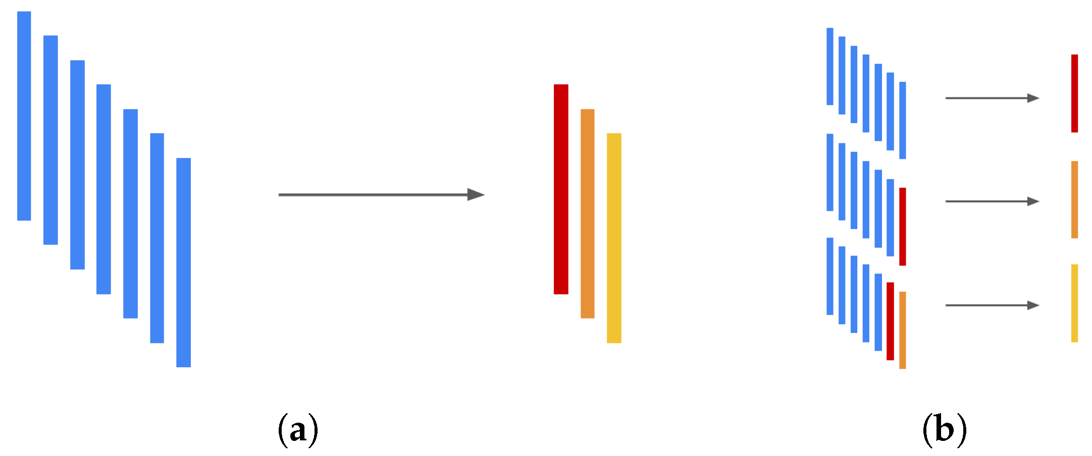
3.7. Regimes
3.8. Implementation
4. Results
4.1. Inputs Configuration
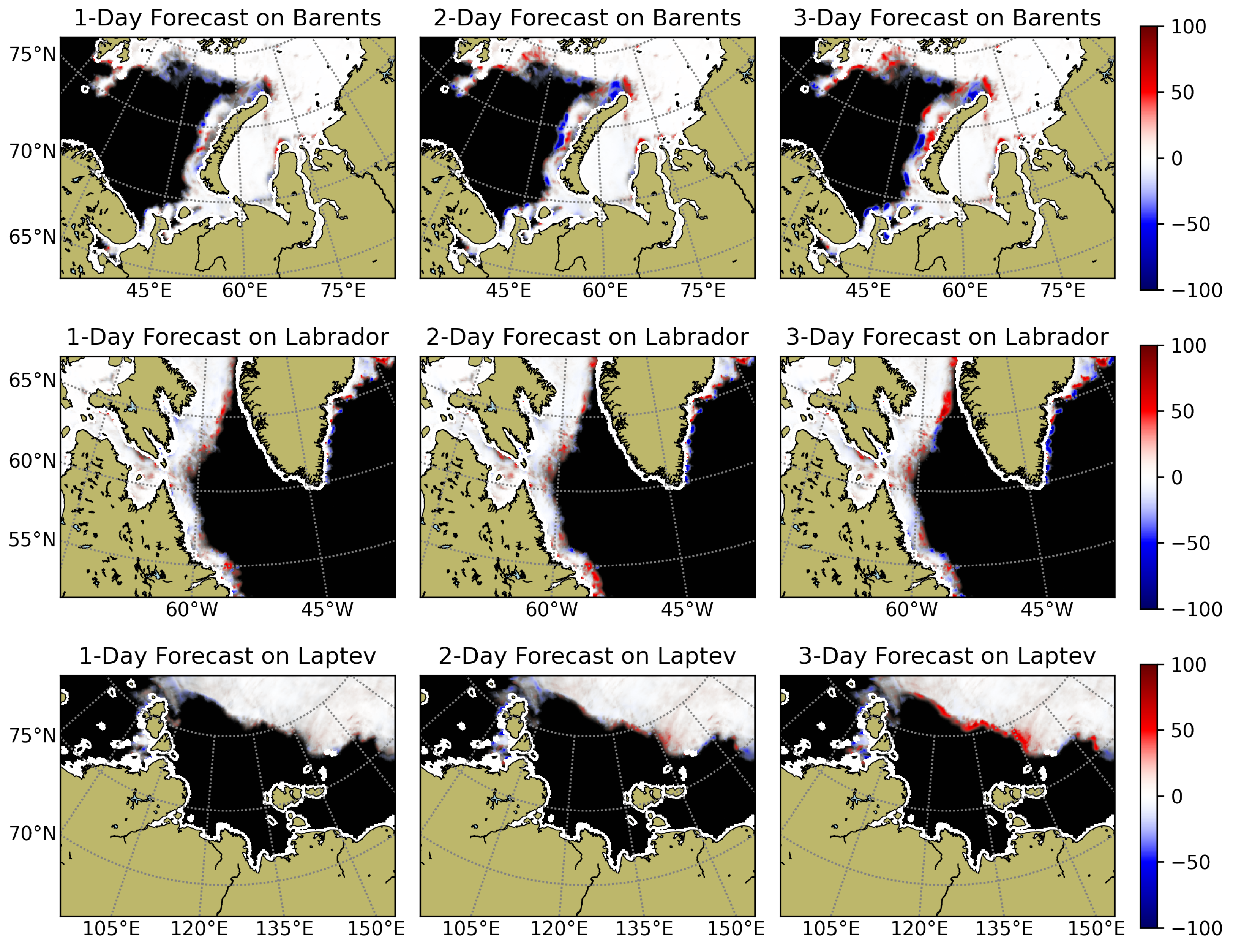
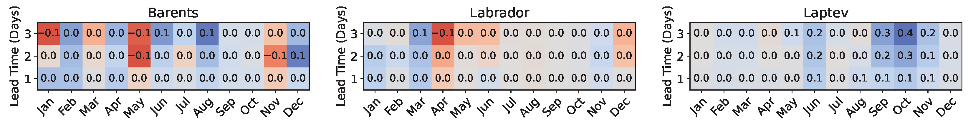
4.2. Predicting Differences with a Baseline
4.3. Pretraining in R-Regime
- 1.
- Pretraining the model in S-regime with ;
- 2.
- Initializing the model with the pretrained checkpoint and tuning it in R-regime for days.
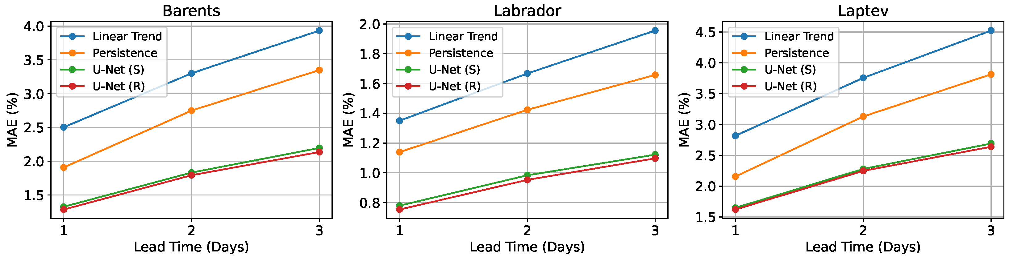
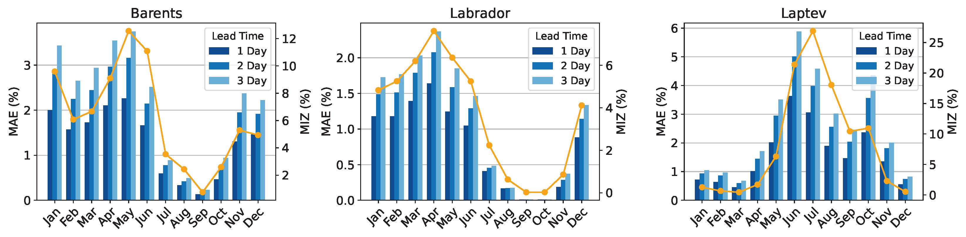
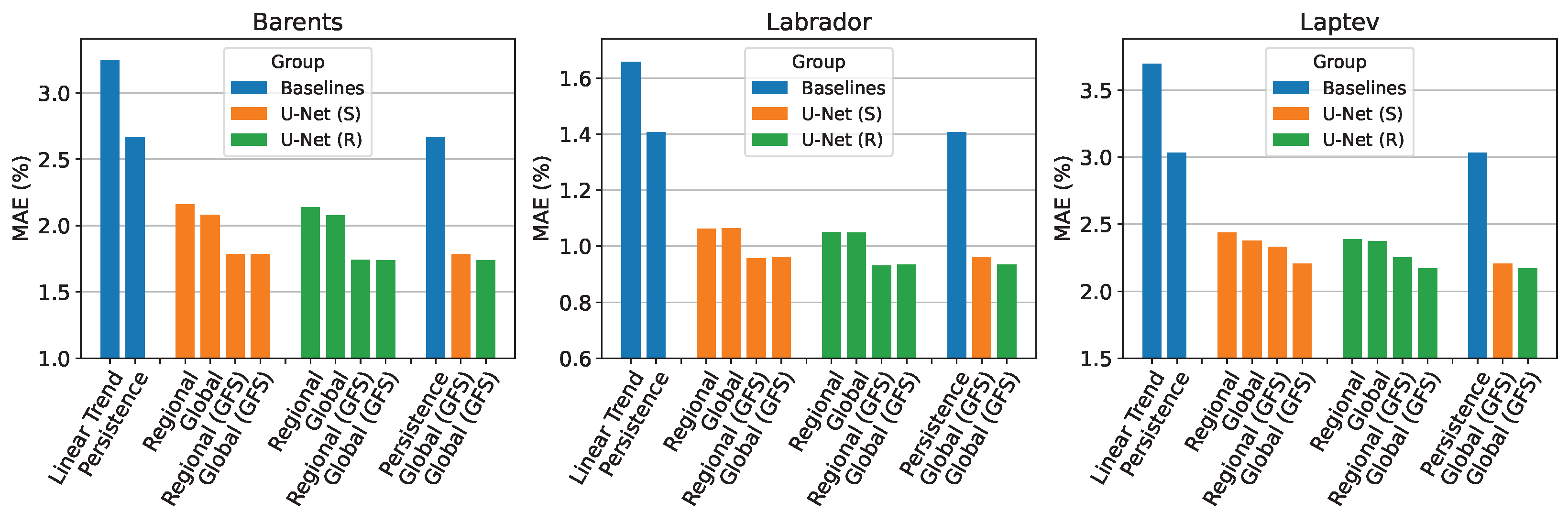
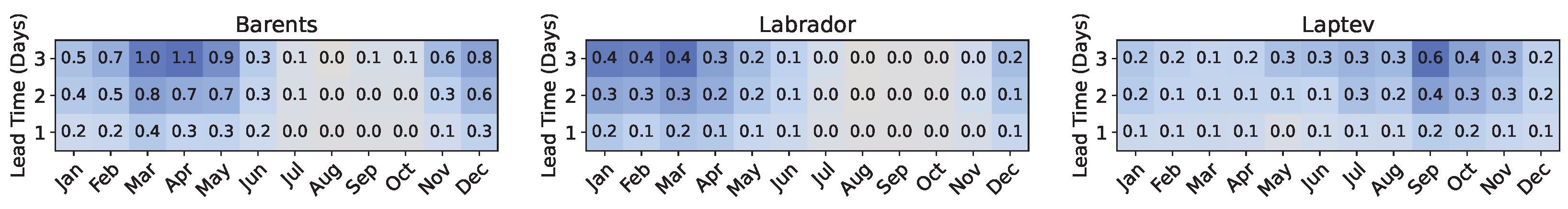
4.4. 3 Days Ahead Forecast
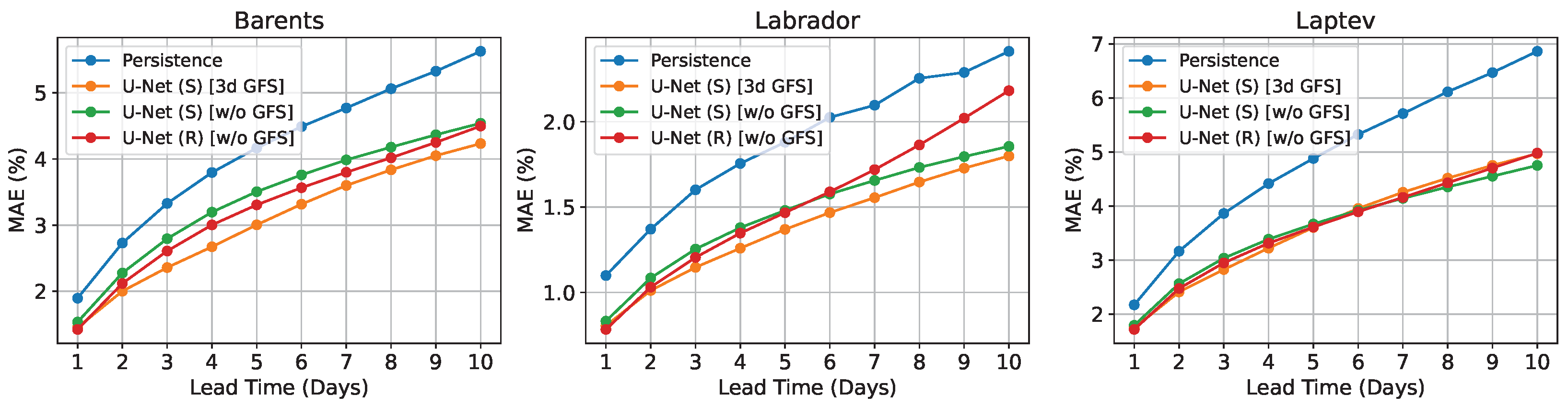
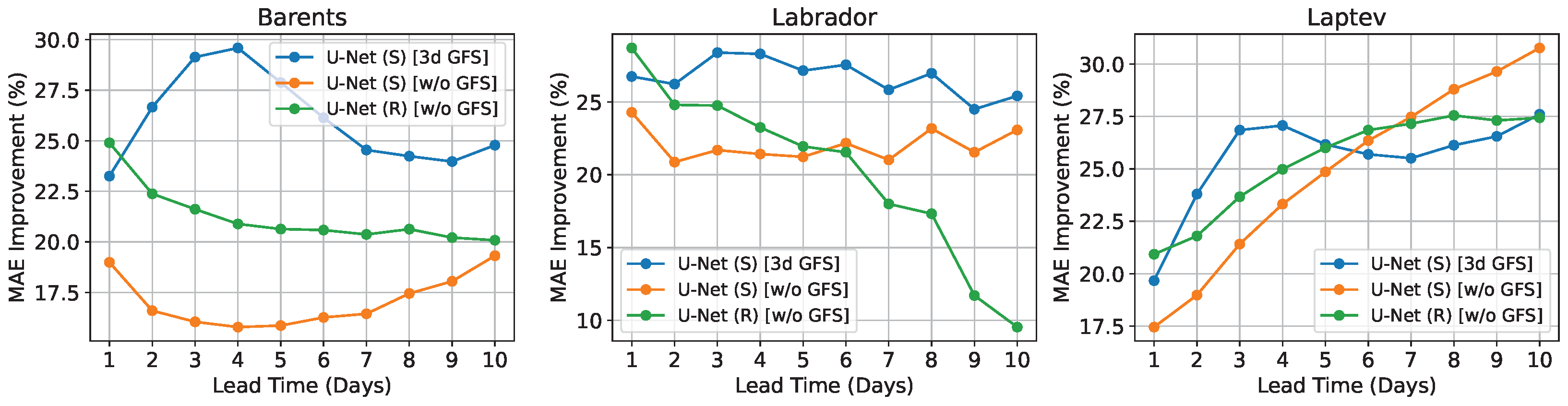
4.5. 10 Days Ahead Forecast
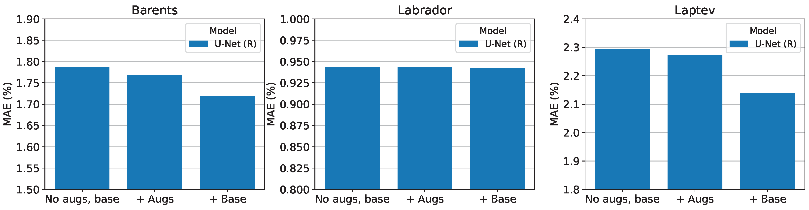
4.6. Ablation Studies
5. Discussion
6. Conclusions
Supplementary Materials
Author Contributions
Funding
Data Availability Statement
Acknowledgments
Conflicts of Interest
Abbreviations
| AMSR-2 | Advanced Microwave Scanning Radiometer 2 |
| CNN | Convolutional neural network |
| CPU | Central processing unit |
| ConvLSTM | Convolutional LSTM |
| DMSP | Defense Meteorological Satellite Program |
| ECMWF | European Centre for Medium-Range Weather Forecasts |
| ERA | ECMWF re-analysis dataset |
| GFS | Global Forecast System |
| GPU | Graphics processing unit |
| GRU | Gated recurrent unit |
| IIEE | Integrated ice edge error |
| JAXA | Japan Aerospace Exploration Agency |
| k-NN | k nearest neighbors |
| LSTM | Long short-term memory |
| MAE | Mean absolute error |
| MIZ | Marginal ice zone |
| MLP | Multilayer perceptron |
| NEMO | Nucleus for European Modelling of the Ocean |
| NOAA | National Oceanic and Atmospheric Administration |
| NSIDC | National Snow and Ice Data Center |
| ORAS4 | Ocean Reanalysis System 4 |
| RF | Random Forest |
| RMSE | Root mean square error |
| RNN | Recurrent neural network |
| SAR | Synthetic-aperture radar |
| SIC | Sea ice concentration |
| SMMR | Scanning multichannel microwave radiometer |
| SSMI | Special Sensor Microwave/Imager |
| SSMIS | Special Sensor Microwave Imager/Sounder |
References
- Screen, J.A.; Simmonds, I. The central role of diminishing sea ice in recent Arctic temperature amplification. Nature 2010, 464, 1334–1337. [Google Scholar] [CrossRef] [PubMed] [Green Version]
- Arndt, D.; Blunden, J.; Willett, K.; Aaron-Morrison, A.P.; Ackerman, S.A.; Adamu, J.; Albanil, A.; Alfaro, E.J.; Allan, R.; Alley, R.B.; et al. State of the climate in 2014. Bull. Am. Meteorol. Soc. 2015, 96, S1–S267. [Google Scholar]
- Blunden, J.; Arndt, D.S. State of the Climate in 2016. Bull. Am. Meteorol. Soc. 2016, 98, Si-S280. [Google Scholar] [CrossRef] [Green Version]
- Hausfather, Z.; Cowtan, K.; Clarke, D.C.; Jacobs, P.; Richardson, M.; Rohde, R. Assessing recent warming using instrumentally homogeneous sea surface temperature records. Sci. Adv. 2017, 3, e1601207. [Google Scholar] [CrossRef] [PubMed] [Green Version]
- You, Q.; Cai, Z.; Pepin, N.; Chen, D.; Ahrens, B.; Jiang, Z.; Wu, F.; Kang, S.; Zhang, R.; Wu, T.; et al. Warming amplification over the Arctic Pole and Third Pole: Trends, mechanisms and consequences. Earth-Sci. Rev. 2021, 217, 103625. [Google Scholar] [CrossRef]
- Kwok, R. Arctic sea ice thickness, volume, and multiyear ice coverage: Losses and coupled variability (1958–2018). Environ. Res. Lett. 2018, 13, 105005. [Google Scholar] [CrossRef]
- Perovich, D.; Smith, M.; Light, B.; Webster, M. Meltwater sources and sinks for multiyear Arctic sea ice in summer. Cryosphere 2021, 15, 4517–4525. [Google Scholar] [CrossRef]
- Renner, A.H.; Gerland, S.; Haas, C.; Spreen, G.; Beckers, J.F.; Hansen, E.; Nicolaus, M.; Goodwin, H. Evidence of Arctic sea ice thinning from direct observations. Geophys. Res. Lett. 2014, 41, 5029–5036. [Google Scholar] [CrossRef] [Green Version]
- Williams, T.; Korosov, A.; Rampal, P.; Ólason, E. Presentation and evaluation of the Arctic sea ice forecasting system neXtSIM-F. Cryosphere 2021, 15, 3207–3227. [Google Scholar] [CrossRef]
- Aseel, S.; Al-Yafei, H.; Kucukvar, M.; Onat, N.C.; Turkay, M.; Kazancoglu, Y.; Al-Sulaiti, A.; Al-Hajri, A. A model for estimating the carbon footprint of maritime transportation of Liquefied Natural Gas under uncertainty. Sustain. Prod. Consum. 2021, 27, 1602–1613. [Google Scholar] [CrossRef]
- Greene, S.; Jia, H.; Rubio-Domingo, G. Well-to-tank carbon emissions from crude oil maritime transportation. Transp. Res. Part Transp. Environ. 2020, 88, 102587. [Google Scholar] [CrossRef]
- Ankathi, S.; Lu, Z.; Zaimes, G.G.; Hawkins, T.; Gan, Y.; Wang, M. Greenhouse gas emissions from the global transportation of crude oil: Current status and mitigation potential. J. Ind. Ecol. 2022. [Google Scholar] [CrossRef]
- Kaleschke, L.; Tian-Kunze, X.; Maaß, N.; Beitsch, A.; Wernecke, A.; Miernecki, M.; Müller, G.; Fock, B.H.; Gierisch, A.M.; Schlünzen, K.H.; et al. SMOS sea ice product: Operational application and validation in the Barents Sea marginal ice zone. Remote Sens. Environ. 2016, 180, 264–273. [Google Scholar] [CrossRef]
- Rampal, P.; Bouillon, S.; Ólason, E.; Morlighem, M. neXtSIM: A new Lagrangian sea ice model. Cryosphere 2016, 10, 1055–1073. [Google Scholar] [CrossRef] [Green Version]
- Rasmus Tonboe, J.L.R.H.P.; Howe, E. Product User Manual for OSI SAF Global Sea Ice Concentration; Product OSI-401-b; Danish Meteorological Institute: Copenhagen, Denmark, 2017. [Google Scholar]
- Lavelle, J.; Tonboe, R.; Tian, T.; Pfeiffer, R.H.; Howe, E. Product User Manual for the OSI SAF AMSR-2 Global Sea Ice Concentration; Product OSI-408; Danish Meteorological Institute: Copenhagen, Denmark, 2016. [Google Scholar]
- Kwok, R.; Cunningham, G. ICESat over Arctic sea ice: Estimation of snow depth and ice thickness. J. Geophys. Res. Oceans 2008, 113. [Google Scholar] [CrossRef]
- Girard, L.; Weiss, J.; Molines, J.M.; Barnier, B.; Bouillon, S. Evaluation of high-resolution sea ice models on the basis of statistical and scaling properties of Arctic sea ice drift and deformation. J. Geophys. Res. Oceans 2009, 114. [Google Scholar] [CrossRef]
- Bouillon, S.; Rampal, P. Presentation of the dynamical core of neXtSIM, a new sea ice model. Ocean Model. 2015, 91, 23–37. [Google Scholar] [CrossRef]
- Girard, L.; Bouillon, S.; Weiss, J.; Amitrano, D.; Fichefet, T.; Legat, V. A new modeling framework for sea-ice mechanics based on elasto-brittle rheology. Ann. Glaciol. 2011, 52, 123–132. [Google Scholar] [CrossRef]
- Sulsky, D.; Schreyer, H.; Peterson, K.; Kwok, R.; Coon, M. Using the material-point method to model sea ice dynamics. J. Geophys. Res. Oceans 2007, 112. [Google Scholar] [CrossRef] [Green Version]
- Fritzner, S.; Graversen, R.; Christensen, K.H.; Rostosky, P.; Wang, K. Impact of assimilating sea ice concentration, sea ice thickness and snow depth in a coupled ocean–sea ice modelling system. Cryosphere 2019, 13, 491–509. [Google Scholar] [CrossRef] [Green Version]
- Fritzner, S.; Graversen, R.; Christensen, K. Assessment of High-Resolution Dynamical and Machine Learning Models for Prediction of Sea Ice Concentration in a Regional Application. J. Geophys. Res. Oceans 2020, 125. [Google Scholar] [CrossRef]
- Koldasbayeva, D.; Tregubova, P.; Shadrin, D.; Gasanov, M.; Pukalchik, M. Large-scale forecasting of Heracleum sosnowskyi habitat suitability under the climate change on publicly available data. Sci. Rep. 2022, 12, 6128. [Google Scholar] [CrossRef] [PubMed]
- Illarionova, S.; Shadrin, D.; Ignatiev, V.; Shayakhmetov, S.; Trekin, A.; Oseledets, I. Estimation of the Canopy Height Model From Multispectral Satellite Imagery With Convolutional Neural Networks. IEEE Access 2022, 10, 34116–34132. [Google Scholar] [CrossRef]
- Illarionova, S.; Shadrin, D.; Ignatiev, V.; Shayakhmetov, S.; Trekin, A.; Oseledets, I. Augmentation-Based Methodology for Enhancement of Trees Map Detalization on a Large Scale. Remote Sens. 2022, 14, 2281. [Google Scholar] [CrossRef]
- LeCun, Y.; Boser, B.; Denker, J.S.; Henderson, D.; Howard, R.E.; Hubbard, W.; Jackel, L.D. Backpropagation Applied to Handwritten Zip Code Recognition. Neural Comput. 1989, 1, 541–551. [Google Scholar] [CrossRef]
- LeCun, Y.; Boser, B.; Denker, J.; Henderson, D.; Howard, R.; Hubbard, W.; Jackel, L. Handwritten Digit Recognition with a Back-Propagation Network. In Advances in Neural Information Processing Systems; Touretzky, D., Ed.; Morgan-Kaufmann: Burlington, MD, USA, 1989; Volume 2. [Google Scholar]
- Lecun, Y.; Bottou, L.; Bengio, Y.; Haffner, P. Gradient-based learning applied to document recognition. Proc. IEEE 1998, 86, 2278–2324. [Google Scholar] [CrossRef] [Green Version]
- Ronneberger, O.; Fischer, P.; Brox, T. U-Net: Convolutional Networks for Biomedical Image Segmentation. arXiv 2015, arXiv:1505.04597. [Google Scholar]
- He, K.; Zhang, X.; Ren, S.; Sun, J. Deep Residual Learning for Image Recognition. In Proceedings of the 2016 IEEE Conference on Computer Vision and Pattern Recognition (CVPR), Las Vegas, NV, USA, 27–30 June 2016; pp. 770–778. [Google Scholar] [CrossRef] [Green Version]
- Hochreiter, S.; Schmidhuber, J. Long short-term memory. Neural Comput. 1997, 9, 1735–1780. [Google Scholar] [CrossRef]
- Cho, K.; Van Merriënboer, B.; Gulcehre, C.; Bahdanau, D.; Bougares, F.; Schwenk, H.; Bengio, Y. Learning phrase representations using RNN encoder-decoder for statistical machine translation. arXiv 2014, arXiv:1406.1078. [Google Scholar]
- Vaswani, A.; Shazeer, N.; Parmar, N.; Uszkoreit, J.; Jones, L.; Gomez, A.N.; Kaiser, L.U.; Polosukhin, I. Attention is All you Need. In Proceedings of the Advances in Neural Information Processing Systems, (NIPS 2017), Long Beach, CA, USA, 4–9 December 2017; Guyon, I., Luxburg, U.V., Bengio, S., Wallach, H., Fergus, R., Vishwanathan, S., Garnett, R., Eds.; Curran Associates, Inc.: Red Hook, NY, USA, 2017; Volume 30. [Google Scholar]
- Jaderberg, M.; Simonyan, K.; Zisserman, A.; Kavukcuoglu, K. Spatial Transformer Networks. In Advances in Neural Information Processing Systems; Cortes, C., Lawrence, N., Lee, D., Sugiyama, M., Garnett, R., Eds.; Curran Associates, Inc.: Red Hook, NY, USA, 2015; Volume 28. [Google Scholar]
- Kim, J.; Kim, K.; Cho, J.; Kang, Y.Q.; Yoon, H.J.; Lee, Y.W. Satellite-Based Prediction of Arctic Sea Ice Concentration Using a Deep Neural Network with Multi-Model Ensemble. Remote Sens. 2019, 11, 19. [Google Scholar] [CrossRef] [Green Version]
- Chi, J.; Kim, H.C. Prediction of Arctic Sea Ice Concentration Using a Fully Data Driven Deep Neural Network. Remote Sens. 2017, 9, 1305. [Google Scholar] [CrossRef] [Green Version]
- Wang, L.; Scott, K.A.; Clausi, D.A. Sea Ice Concentration Estimation during Freeze-Up from SAR Imagery Using a Convolutional Neural Network. Remote Sens. 2017, 9, 408. [Google Scholar] [CrossRef]
- Kim, Y.J.; Kim, H.C.; Han, D.; Lee, S.; Im, J. Prediction of monthly Arctic sea ice concentrations using satellite and reanalysis data based on convolutional neural networks. Cryosphere 2020, 14, 1083–1104. [Google Scholar] [CrossRef] [Green Version]
- Liu, Y.; Bogaardt, L.; Attema, J.; Hazeleger, W. Extended Range Arctic Sea Ice Forecast with Convolutional Long-Short Term Memory Networks. Mon. Weather Rev. 2021, 149, 1673–1693. [Google Scholar] [CrossRef]
- Andersson, T.R.; Hosking, J.S.; Pérez-Ortiz, M.; Paige, B.; Elliott, A.; Russell, C.; Law, S.; Jones, D.C.; Wilkinson, J.; Phillips, T.; et al. Seasonal Arctic sea ice forecasting with probabilistic deep learning. Nat. Commun. 2021, 12, 5124. [Google Scholar] [CrossRef]
- Shi, X.; Chen, Z.; Wang, H.; Yeung, D.Y.; Wong, W.K.; Woo, W.C. Convolutional LSTM Network: A Machine Learning Approach for Precipitation Nowcasting. In Proceedings of the 28th International Conference on Neural Information Processing Systems, NIPS’15, Sanur, Bali, Indonesia, 8–12 December 2021; MIT Press: Cambridge, MA, USA, 2015; Volume 1, pp. 802–810. [Google Scholar]
- Choi, M.; De Silva, L.W.A.; Yamaguchi, H. Artificial Neural Network for the Short-Term Prediction of Arctic Sea Ice Concentration. Remote Sens. 2019, 11, 1071. [Google Scholar] [CrossRef] [Green Version]
- Liu, Q.; Zhang, R.; Wang, Y.; Yan, H.; Hong, M. Daily Prediction of the Arctic Sea Ice Concentration Using Reanalysis Data Based on a Convolutional LSTM Network. J. Mar. Sci. Eng. 2021, 9, 330. [Google Scholar] [CrossRef]
- Liu, Q.; Ren, Z.; Yangjun, W.; Yan, H.; Hong, M. Short-Term Daily Prediction of Sea Ice Concentration Based on Deep Learning of Gradient Loss Function. Front. Mar. Sci. 2021, 8, 736429. [Google Scholar] [CrossRef]
- Wang, Y.; Gao, Z.; Long, M.; Wang, J.; Yu, P.S. PredRNN++: Towards A Resolution of the Deep-in-Time Dilemma in Spatiotemporal Predictive Learning. In Proceedings of the 35th International Conference on Machine Learning, Stockholm, Sweden, 10–15 July 2018; Dy, J., Krause, A., Eds.; Proceedings of Machine Learning Research. Volume 80, pp. 5123–5132. [Google Scholar]
- Kern, S.; Lavergne, T.; Notz, D.; Pedersen, L.T.; Tonboe, R. Satellite passive microwave sea-ice concentration data set inter-comparison for Arctic summer conditions. Cryosphere 2020, 14, 2469–2493. [Google Scholar] [CrossRef]
- Kern, S.; Lavergne, T.; Notz, D.; Pedersen, L.T.; Tonboe, R.T.; Saldo, R.; Sørensen, A.M. Satellite passive microwave sea-ice concentration data set intercomparison: Closed ice and ship-based observations. Cryosphere 2019, 13, 3261–3307. [Google Scholar] [CrossRef] [Green Version]
- Cavalieri, D.; Parkinson, C.; Vinnikov, K.Y. 30-Year satellite record reveals contrasting Arctic and Antarctic decadal sea ice variability. Geophys. Res. Lett. 2003, 30. [Google Scholar] [CrossRef] [Green Version]
- Wagner, P.M.; Hughes, N.; Bourbonnais, P.; Stroeve, J.; Rabenstein, L.; Bhatt, U.; Little, J.; Wiggins, H.; Fleming, A. Sea-ice information and forecast needs for industry maritime stakeholders. Polar Geogr. 2020, 43, 160–187. [Google Scholar] [CrossRef]
- Hunke, E.; Allard, R.; Blain, P.; Blockley, E.; Feltham, D.; Fichefet, T.; Garric, G.; Grumbine, R.; Lemieux, J.F.; Rasmussen, T.; et al. Should sea-ice modeling tools designed for climate research be used for short-term forecasting? Curr. Clim. Chang. Rep. 2020, 6, 121–136. [Google Scholar] [CrossRef] [PubMed]
- Blockley, E.; Vancoppenolle, M.; Hunke, E.; Bitz, C.; Feltham, D.; Lemieux, J.F.; Losch, M.; Maisonnave, E.; Notz, D.; Rampal, P.; et al. The future of sea ice modeling: Where do we go from here? Bull. Am. Meteorol. Soc. 2020, 101, E1304–E1311. [Google Scholar] [CrossRef]
- Lu, J.; Heygster, G.; Spreen, G. Atmospheric correction of sea ice concentration retrieval for 89 GHz AMSR-E observations. IEEE J. Sel. Top. Appl. Earth Obs. Remote Sens. 2018, 11, 1442–1457. [Google Scholar] [CrossRef]
- National Centers for Environmental Prediction; National Weather Service, NOAA; U.S. Department of Commerce. NCEP GFS 0.25 Degree Global Forecast Grids Historical Archive; University Corporation for Atmospheric Research: Boulder, CO, USA, 2015. [Google Scholar]
- Ioffe, S.; Szegedy, C. Batch Normalization: Accelerating Deep Network Training by Reducing Internal Covariate Shift. In Proceedings of the 32nd International Conference on Machine Learning-JMLR.org, ICML’15, Lille, France, 6–11 July 2015; Volume 37, pp. 448–456. [Google Scholar]
- Goessling, H.F.; Tietsche, S.; Day, J.J.; Hawkins, E.; Jung, T. Predictability of the Arctic sea ice edge. Geophys. Res. Lett. 2016, 43, 1642–1650. [Google Scholar] [CrossRef] [Green Version]
- Shorten, C.; Khoshgoftaar, T.M. A survey on Image Data Augmentation for Deep Learning. J. Big Data 2019, 6, 60. [Google Scholar] [CrossRef]
- Hochreiter, S. The Vanishing Gradient Problem During Learning Recurrent Neural Nets and Problem Solutions. Int. J. Uncertain. Fuzziness-Knowl. Syst. 1998, 6, 107–116. [Google Scholar] [CrossRef] [Green Version]
- Bengio, Y.; Louradour, J.; Collobert, R.; Weston, J. Curriculum Learning. In Proceedings of the 26th Annual International Conference on Machine Learning, ICML ’09, Montreal, QC, Canada, 14–18 June 2009; Association for Computing Machinery: New York, NY, USA, 2009; pp. 41–48. [Google Scholar] [CrossRef]
- Kumar, S. On weight initialization in deep neural networks. arXiv 2017, arXiv:1704.08863. [Google Scholar]
- Uotila, P.; Goosse, H.; Haines, K.; Chevallier, M.; Barthélemy, A.; Bricaud, C.; Carton, J.; Fučkar, N.; Garric, G.; Iovino, D.; et al. An assessment of ten ocean reanalyses in the polar regions. Clim. Dyn. 2019, 52, 1613–1650. [Google Scholar] [CrossRef]
- Wang, Y.; Long, M.; Wang, J.; Gao, Z.; Yu, P.S. PredRNN: Recurrent Neural Networks for Predictive Learning using Spatiotemporal LSTMs. In Advances in Neural Information Processing Systems; Guyon, I., Luxburg, U.V., Bengio, S., Wallach, H., Fergus, R., Vishwanathan, S., Garnett, R., Eds.; Curran Associates, Inc.: Red Hook, NY, USA, 2017; Volume 30. [Google Scholar]
- Wang, u.; Wu, H.; Zhang, J.; Gao, Z.; Wang, J.; Yu, P.; Long, M. PredRNN: A Recurrent Neural Network for Spatiotemporal Predictive Learning; IEEE Transactions on Pattern Analysis and Machine Intelligence: Manhattan, NY, USA, 2021. [Google Scholar]
- Wang, Y.; Jiang, L.; Yang, M.H.; Li, L.J.; Long, M.; Fei-Fei, L. Eidetic 3D LSTM: A Model for Video Prediction and Beyond. In Proceedings of the ICLR, New Orleans, LA, USA, 6–9 May 2019. [Google Scholar]
- Yu, W.; Lu, Y.; Easterbrook, S.M.; Fidler, S. Efficient and Information-Preserving Future Frame Prediction and Beyond. In Proceedings of the ICLR, Addis Ababa, Ethiopia, 26–30 April 2020. [Google Scholar]
- Chen, R.T.Q.; Rubanova, Y.; Bettencourt, J.; Duvenaud, D.K. Neural Ordinary Differential Equations. In Proceedings of the Advances in Neural Information Processing Systems, Long Beach, CA, USA, 4–9 December 2017; Bengio, S., Wallach, H., Larochelle, H., Grauman, K., Cesa-Bianchi, N., Garnett, R., Eds.; Curran Associates, Inc.: Red Hook, NY, USA, 2018; Volume 31. [Google Scholar]
- Puy, G.; Boulch, A.; Marlet, R. FLOT: Scene Flow on Point Clouds Guided by Optimal Transport. In Proceedings of the European Conference on Computer Vision, Glasgow, UK, 23–28 August 2020. [Google Scholar]
- Rout, L.; Korotin, A.; Burnaev, E. Generative Modeling with Optimal Transport Maps. In Proceedings of the International Conference on Learning Representations, Virtual, 25 April 2022. [Google Scholar]


| Parameter Name | Value | Unit |
|---|---|---|
| Projection | Lambert Azimuthal Equal Area | - |
| Grid step | 5 | km |
| Grid Height | 360 | knot |
| 1800 | km | |
| Grid Width | 500 | knot |
| 2500 | km |
| Region | Central Point (Lat, Lon) | Presentation Percentage |
|---|---|---|
| Barents | 73°, 57.3° | 56.82% |
| Labrador | 61°, −56° | 47.84% |
| Laptev | 76°, 125° | 51.53% |
| Source | Channel | Preprocessing | Time Interval |
|---|---|---|---|
| JAXA | SIC | Data | Past |
| GFS | Temperature | Climatology | Today |
| Temperature | Clim. Anomaly | Today | |
| Temperature | Clim. Anomaly | Future | |
| Pressure | Climatology | Today | |
| Pressure | Clim. Anomaly | Today | |
| Pressure | Clim. Anomaly | Future | |
| Wind (u) | Data | Today | |
| Wind (u) | Data | Future | |
| Wind (v) | Data | Today | |
| Wind (v) | Data | Future | |
| Wind (module) | Data | Today | |
| Wind (module) | Data | Future | |
| General | Date (cos) | Data | Today |
| Date (sin) | Data | Today | |
| Land | Data | Today |
| Linear Trend | Persistence | U-Net (S) | U-Net (R) | ||
|---|---|---|---|---|---|
| Region | Metric | ||||
| Barents | IIEE | 2.96 | 2.46 | 1.48 ± 0.02 | 1.41 ± 0.009 |
| MAE | 3.25 | 2.67 | 1.78 ± 0.01 | 1.73 ± 0.004 | |
| RMSE | 9.8 | 8.44 | 5.68 ± 0.05 | 5.51 ± 0.05 | |
| Labrador | IIEE | 1.82 | 1.54 | 0.905 ± 0.004 | 0.871 ± 0.01 |
| MAE | 1.66 | 1.41 | 0.966 ± 0.003 | 0.939 ± 0.009 | |
| RMSE | 6.59 | 6.02 | 3.96 ± 0.03 | 3.88 ± 0.05 | |
| Laptev | IIEE | 2.03 | 1.7 | 1.11 ± 0.03 | 1.05 ± 0.02 |
| MAE | 3.7 | 3.03 | 2.22 ± 0.02 | 2.16 ± 0.007 | |
| RMSE | 8.87 | 7.61 | 5.1 ± 0.06 | 4.98 ± 0.05 |
Publisher’s Note: MDPI stays neutral with regard to jurisdictional claims in published maps and institutional affiliations. |
© 2022 by the authors. Licensee MDPI, Basel, Switzerland. This article is an open access article distributed under the terms and conditions of the Creative Commons Attribution (CC BY) license (https://creativecommons.org/licenses/by/4.0/).
Share and Cite
Grigoryev, T.; Verezemskaya, P.; Krinitskiy, M.; Anikin, N.; Gavrikov, A.; Trofimov, I.; Balabin, N.; Shpilman, A.; Eremchenko, A.; Gulev, S.; et al. Data-Driven Short-Term Daily Operational Sea Ice Regional Forecasting. Remote Sens. 2022, 14, 5837. https://doi.org/10.3390/rs14225837
Grigoryev T, Verezemskaya P, Krinitskiy M, Anikin N, Gavrikov A, Trofimov I, Balabin N, Shpilman A, Eremchenko A, Gulev S, et al. Data-Driven Short-Term Daily Operational Sea Ice Regional Forecasting. Remote Sensing. 2022; 14(22):5837. https://doi.org/10.3390/rs14225837
Chicago/Turabian StyleGrigoryev, Timofey, Polina Verezemskaya, Mikhail Krinitskiy, Nikita Anikin, Alexander Gavrikov, Ilya Trofimov, Nikita Balabin, Aleksei Shpilman, Andrei Eremchenko, Sergey Gulev, and et al. 2022. "Data-Driven Short-Term Daily Operational Sea Ice Regional Forecasting" Remote Sensing 14, no. 22: 5837. https://doi.org/10.3390/rs14225837