Article

Improvement of the SWAT Model for Snowmelt Runoff Simulation in Seasonal Snowmelt Area Using Remote Sensing Data

1
College of New Energy and Environment, Jilin University, Changchun 130021, China
2
Key Laboratory of Groundwater Resources and Environment, Ministry of Education, Jilin University, Changchun 130021, China
3
Jilin Provincial Key Laboratory of Water Resources and Environment, Jilin University, Changchun 130021, China
4
Department of Civil Engineering, Swansea University Bay Campus, Fabian Way, Swansea SA1 8EN, UK
*
Author to whom correspondence should be addressed.
Remote Sens. 2022, 14(22), 5823; https://doi.org/10.3390/rs14225823
Submission received: 10 October 2022 / Revised: 11 November 2022 / Accepted: 15 November 2022 / Published: 17 November 2022

Abstract

:
The SWAT model has been widely used to simulate snowmelt runoff in cold regions thanks to its ability of representing the effects of snowmelt and permafrost on runoff generation and confluence. However, a core method used in the SWAT model, the temperature index method, assumes both the dates for maximum and minimum snowmelt factors and the snowmelt temperature threshold, which leads to inaccuracies in simulating snowmelt runoff in seasonal snowmelt regions. In this paper, we present the development and application of an improved temperature index method for SWAT (SWAT+) in simulating the daily snowmelt runoff in a seasonal snowmelt area of Northeast China. The improvements include the introduction of total radiation to the temperature index method, modification of the snowmelt factor seasonal variation formula, and changing the snowmelt temperature threshold according to the snow depth derived from passive microwave remote sensing data and temperature in the seasonal snowmelt area. Further, the SWAT+ model is applied to study climate change impact on future snowmelt runoff (2025–2054) under the climate change scenarios including SSP2.6, SSP4.5, and SSP8.5. Much improved snowmelt runoff simulation is obtained as a result, supported by several metrics, such as MAE, RE, RMSE, R2, and NSE for both the calibration and validation. Compared with the baseline period (1980–2019), the March–April ensemble average snowmelt runoff is shown to decrease under the SSP2.6, SSP4.5, and SSP8.5 scenario during 2025–2054. This study provides a valuable insight into the efficient development and utilization of spring water resources in seasonal snowmelt areas.

1. Introduction

Snowmelt runoff is an essential component of water resources in many parts of the world [1]. At the same time, it may become a disaster in the form of a snowmelt flood under certain conditions [2]. Accurate simulation and prediction of snowmelt runoff are crucial in water resources management and snowmelt flood disaster prevention [3,4]. Naturally, snowmelt runoff is affected by a variety of meteorological factors and involves many complex physical processes [5]; as such, modeling snowmelt runoff is more challenging than that for conventional rainfall-runoff processes [6,7]. These challenges become even more exacerbated when it comes to representing the climate change impact on hydrological processes [8,9].
Many researchers have attempted to develop snowmelt runoff models directly or to add snowmelt modules to existing hydrological models in order to properly simulate snowmelt runoff, including, for example, HBV [10,11], SRM [12,13], UBC [14,15], CRHM [16,17], ARHYTHM [18], and SWAT model [19,20], to name just a few. Among them, the soil and water assessment tool (SWAT) model has been widely used for both simulating and predicting snowmelt runoff, as it considers the impact of snowmelt and frozen soil on runoff generation and concentration [21,22,23].
The SWAT model has a dedicated snowmelt module, which considers only the impact of snowpack temperature and air temperature on snowmelt [24,25]. This often leads to underestimating snowmelt runoff [26]. Some attempts have been made to address this problem, for example, by integrating an energy balance snowmelt model into the SWAT model [27,28]. A clear drawback of this approach is that it often requires extra large amounts of data for parameterization and, when such requirement cannot be met, results from the energy balance model can become worse than other simpler methods [29,30]. Meanwhile, others tried to improve the temperature index method, for example, by including the radiation factor [31,32,33] on the ground that radiation is one of the main energy sources of snow melting [34,35,36]. It is further argued that solar radiation is fundamentally more influential compared with the temperature, as part of the solar radiation energy is used to warm the snow up and the rest to melt the snow [37]. In other words, the snowmelt process is under joint influences of both temperature and solar radiation [35]. From this perspective, research added direct solar radiation to the temperature index method to simulate snowmelt runoff and achieved good results [38]. Apart from direct solar radiation, scattering radiation is also important for snowmelt [39]. Accordingly, adding total radiation on the snow surface into the SWAT model is worth trying to mitigate the snowmelt runoff underestimation problem.
Another perspective from which the snowmelt module of the SWAT model can be improved is related to an important parameter, i.e., the snowmelt factor, which varies seasonally [40]. In the existing setting, the seasonal variation in the snowmelt factor is approximated using a sinusoidal function, which assumes the minima and maxima to be on the 21 December and 21 June, respectively [41]. Clearly, this is not an even close approximation for snowmelt, as snowmelt mainly occurs in spring in many seasonal snowmelt areas [42,43]. In addition, the snowmelt factor decreases as the snow depth reduces [44] and, consequently, the maximum snowmelt rate in the seasonal snowmelt area in the northern hemisphere occurs in late spring [45]. In other words, the assumption with respect to the snowmelt factor is not well supported by the actual processes, which may be a key factor for the low accuracy of snowmelt runoff simulations in the SWAT model. Some researchers proposed using discharge for snowmelt factor determination [46]. However, there is a large time difference between the snowmelt occurrence and snowmelt runoff occurrence in mountainous areas with long confluence time [47,48]. Therefore, in this study, we chose to use the snowmelt occurrence time directly so as to avoid the interference caused by long confluence time.
In addition to the snowmelt factor, another important parameter in the snowmelt module is the snowmelt temperature threshold whose default value is set as 0 °C [49]. Some studies suggested that only 0 °C is not necessarily a best threshold value to determine whether the snow melts. In addition, they advised using the so-called accumulated temperature, which, instead of using a single observed temperature value, determines whether snowmelt occurs by using the sum of all temperature readings in a day that are greater than 0 °C [38,46,50,51]. However, the study ignored the possibility that snowmelt could also occur below 0 °C [52]. The threshold of snowmelt temperature is also closely related to the geographical environment. For example, the snowmelt temperature threshold is found to be below 0 °C in Altay Mountains [53] but well above 0 °C in central Switzerland [54]. Therefore, accurately determining the snowmelt temperature threshold by considering the characteristics of the regional geographical environment needs to be addressed.
Although previous studies have noticed the deficiencies in the existing snowmelt module of SWAT in terms of no consideration of solar radiation, inaccurate snowmelt temperature threshold determination, and no representation of the regional variation in snowmelt factor [38,46,50,51], no attempts have been made to address them in a comprehensive manner. In the study presented in this paper, we systematically addressed these issues by (i) integrating both direct solar radiation and scattering radiation into the temperature index; (ii) using local observations to determine the dates of the maxima and minima of snowmelt factors and modify accordingly the snowmelt factor seasonal variation formula; (iii) determining the temperature threshold of snow melting by identifying the relationship between snow depth and temperature and changing the original temperature threshold; and, (iv) finally, applying the modified model in predicting snowmelt runoff in the study area—the Baishan basin. To facilitate discussion, the modified SWAT model is hereafter referred to as SWAT+.
This paper is structured as follows: Section 2 describes the study area and the data used; Section 3 presents the overall methodology and discusses the details of the improvements made towards the snowmelt module and the bias correction measures in utilizing climate projection data. The results are explained and discussed in Section 4 and Section 5. Finally, the conclusions drawn from this study are presented in Section 6.

2. Materials

2.1. Study Area

Located in the northeast of China (126°28′–128°51′ E, 41°42′–43°21′ N), the Baishan basin is a typical seasonal snowmelt area (Figure 1). The Baishan basin is the main source area of the Second Songhua River, which originates from the Changbaishan Tianchi and consists of two major tributaries: the Toudao Songhua river and the Erdao Songhua river, with a total drainage area of 18,645.4 km2. Snowmelt runoff is a major contribution to the spring water resources in the Baishan basin, lasting from March to April annually [55]. Spring floods often occur when there is a continuing and rapid rise in temperature in spring. According to the long time series of daily snow depth derived from passive microwave remote sensing data provided by the National Qinghai Tibet Plateau data center [56,57], the timing of the first stable snowfalls in the basin ranges from 5 November to 11 November over the 40-year period of 1980–2019, with an averaged starting time of 9 November. The snow cover can last up to 6 months, with the maximum daily snowfall depth up to 24.64 mm. The main snowmelt start time is from 2 March to 14 March.

2.2. Data

Several types of data are used in this study, including spatial data, historical meteorological and hydrological observations, and climate projections. The spatial data consist of digital elevation model (DEM) (obtained from http://www.gscloud.cn website, accessed on 22 December 2021), soil map, and land use. The soil map and land use data come with a spatial resolution of 1 km and are collected from the harmonized world soil database (version 1.1) (http://www.fao.org/soils-portal/data-hub/soil-maps-and-databases/harmonized-world-soil-database-v12, accessed on 25 December 2021) and resource and the environment science data center website (https://www.resdc.cn/, accessed on 15 January 2022), respectively. The historical meteorological and hydrological observations used in the study include daily precipitation, air temperature, wind speed, relative humidity, total solar radiation, the snow depth at three gauged meteorological stations (Jingyu, Donggang, and Songjiang), and discharge from the Baishan reservoir from 1980 to 2019. They were obtained from the National Meteorological Science Data Center (https://data.cma.cn, accessed on 15 January 2022), the National Qinghai Tibet Plateau data center (http://data.tpdc.ac.cn, accessed on 5 April 2022), and Baishan hydropower plant of State Grid Xinyuan company, respectively. Among them, the snow depth is inverted using passive microwave remote sensing, which has also been used in much climate and hydrological research in China [58,59,60] and proved well applicable in Northeast China [61].
Climate projection data from the Coupled Model Intercomparison Project (CMIP6) (http://cmip-pcmdi.llnl.gov/cmip6/, accessed on 3 July 2022), i.e., the BCC-CSM2-MR (Beijing Climate Center/China) model, are selected for future snowmelt runoff changes analysis. The baseline period is set as 1980–2019 and the future period is 2025–2054. There are three different climate change scenarios considered, i.e., SSP2.6, SSP4.5, and SSP8.5, representing sustainable development, moderate development, and conventional development, with the artificial radiation force reaching 2.6, 4.5, and 8.5 W/m2, respectively [62,63].

3. Methods

3.1. Modification and Improvement of the SWAT Model

This section presents the modification made to the original SWAT model, aiming to improve its snowmelt runoff simulation performance. The changes are based on the revision 682 of the SWAT source code (https://bitbucket.org/blacklandgrasslandmodels/swat_development/src/master, accessed on 3 March 2022). The modifications focus on the three components of the snowmelt module in SWAT, i.e., snowmelt calculation taking into account the contribution from radiation, snowmelt factor with more accurate seasonal representation, and snowmelt threshold temperature determined by the local environment.

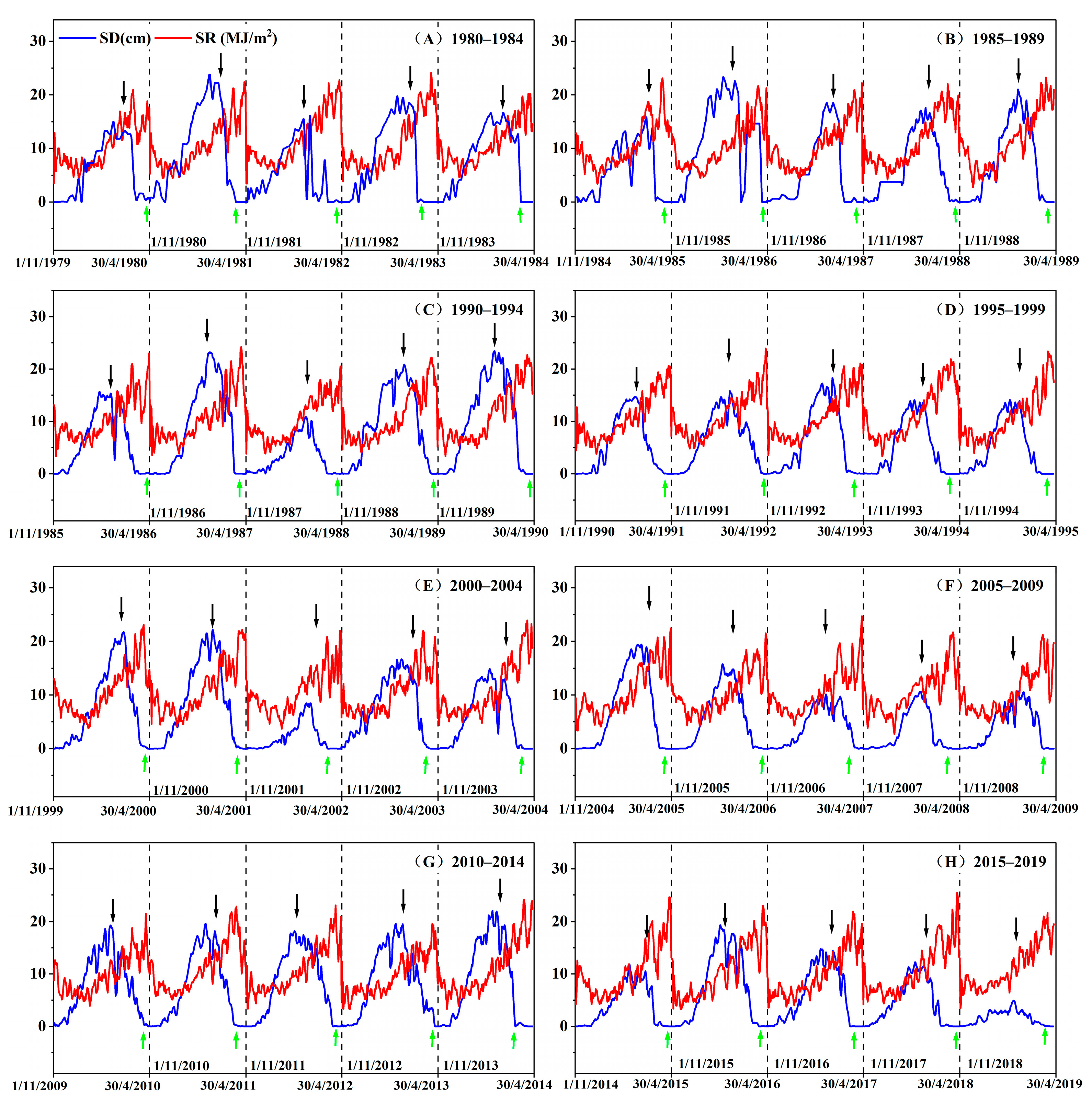
3.1.1. Snowmelt Calculation Considering Total Solar Radiation

In the original SWAT snowmelt module, the change in snowpack depends on sublimation, melting, and snowfall, which is described as the snow water equivalent (SWE), representing water stored in the snowpack. The SWE is calculated as follows:
SWE i = SWE i 1 + P E SM
where SWE i and SWE i 1 are the water content of the snowpack (mm) on the day and the day before; P , E   , and SM are the snowfall (mm), sublimation (mm), and snowmelt (mm), respectively. Snowmelt ( SM ) in the original SWAT model is calculated using the temperature index method, i.e.:
SM = SMF × sno cov × T snow + T mx 2 T mlt
where SMF is the snowmelt factor (mm H2O d−1·°C−1). sno cov is the snow cover fraction. Some studies simulated and predicted snow cover fraction through evolutionary algorithm [64]. In SWAT model, sno cov is calculated based on water content of the snow pack using Equation (3). T snow , T mx , and T mlt is the snowpack temperature, maximum air temperature, and snowmelt temperature threshold (°C), respectively.
sno cov = SNO SNO 100 × SNO SNO 100 + exp cov 1 cov 2 × SNO SNO 100 1
where SNO is the water content of the snow pack on a given day (mm H2O), SNO 100 is the threshold depth of snow at 100% coverage (mm H2O), and cov 1 and cov 2 are coefficients that define the shape of the curve. The values used for cov 1 and cov 2 are determined by solving Equation (3) using two known points: 95% coverage at 95% SNO 100 and 50% coverage at a user-specified fraction of SNO 100 .
Given the important role of solar radiation in the snowmelt process, some researchers have added solar radiation to the classical temperature index method [65,66] and reported improved accuracy in snowmelt simulations. We derived a similar approach in this study and introduced the total solar radiation to the original snowmelt module of the SWAT model. Now the snowmelt is calculated using a modified equation as shown in Equation (4):
SM = sno cov × SMF × T snow + T mx 2 T mlt + SR × 1 α × m Q
where SR is the incoming total solar radiation (W/m2), α is snow albedo, and m Q is the coefficient of energy to water depth conversion. Following a previous study [67], we chose to use α = 0.679, m Q = 0.26 mm·W−1·m2·day−1.

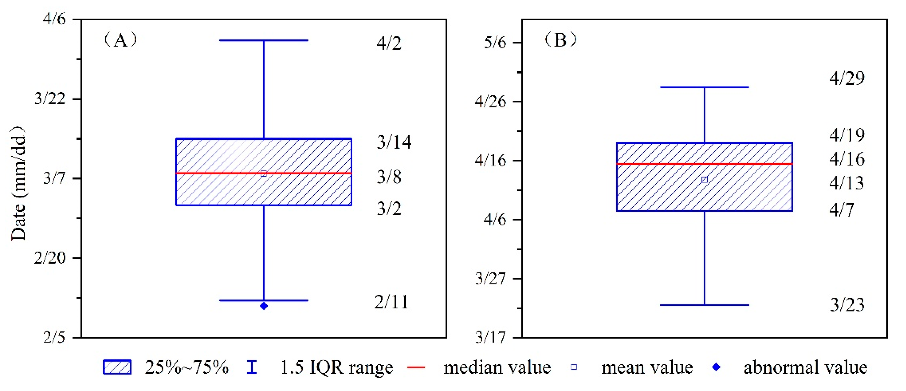
3.1.2. Snowmelt Factor with an Improved Representation of Seasonal Variation

The snowmelt factor (SMF) in the snowmelt module of the SWAT model already considers the seasonal variation, as shown in Equation (5):
SMF = ( SMF 6 + SMF 12 ) 2 + ( SMF 6 SMF 12 ) 2 × sin ( 2 π 365 × ( n 81 ) )
where SMF6 and SMF12 represent the snowmelt factor on the 21 June (172nd day) and the snowmelt factor on 21 December (the 355th day in a year), respectively, that is, when n = 172 and n = 355, 2π/365 × (n − 81) reaches π/2 and 3π/2 phases, respectively. The sin(2π/365 × (n − 81)) formula accordingly reaches maximum values of 1 and minimum values of −1. In addition, n is the order position of the day in a year, i.e., the nth day. In other words, the maximum and the minimum snowmelt factors are assumed to happen on the two fixed dates, which is clearly unfit for seasonal snowmelt basins where solar radiation is an important element affecting the snowmelt rate [68].
In this study, instead of using the two fixed dates, we attempted to determine a more accurate representation of the seasonal variation in the snowmelt factor by, firstly, investigating the relationship between the 5-day moving average of snow depth and temperature from November to April. As shown in Figure 2, the snow depth decreases as the radiation gradually rises. The black arrows indicate the time when the minimum snowmelt factor occurs [69]. Conversely, when the snow depth gradually decreases, the time corresponding to the maximum radiation will be the time of the maximum snowmelt factor, as indicated by the green arrows in Figure 2.
Then, the multi-year average occurrence time for the maxima and minima of the snowmelt factor is obtained by examining the temporal distributions of the two dates, i.e., using a box plot. As shown in Figure 3A, the median date of the snowmelt factor minima is 8 March (the 67th day in a year) and that for the maximum snowmelt factor is 16 April (the 107th day) (Figure 3B). In this study, these two medians are used to represent the maximum and minimum snowmelt factors. Following the sinusoidal variation principle, the formula of the snowmelt factor is modified as Equation (6). The minimum sinusoidal value and maximum sinusoidal value occur when the values of 67 and 107 are substituted into the formula, respectively. That is, when n = 67, the sin function should be in the 3 π / 2 phase and the sinusoidal value should be −1. Meanwhile, the sin function is π / 2 phase and sinusoidal value is 1 for n = 107. Based on this, the formula of the snowmelt factor is modified as follows:
SMF = SMF 3 + SMF 4 2 + SMF 4 SMF 3 2 × sin ( 9 π 365 × 128 n )
where SMF 3   is the snowmelt factor on 8 March and SMF 4 is the snowmelt factor on 16 April, that is, the largest and minimum snowmelt factors in the seasonal snowmelt areas.

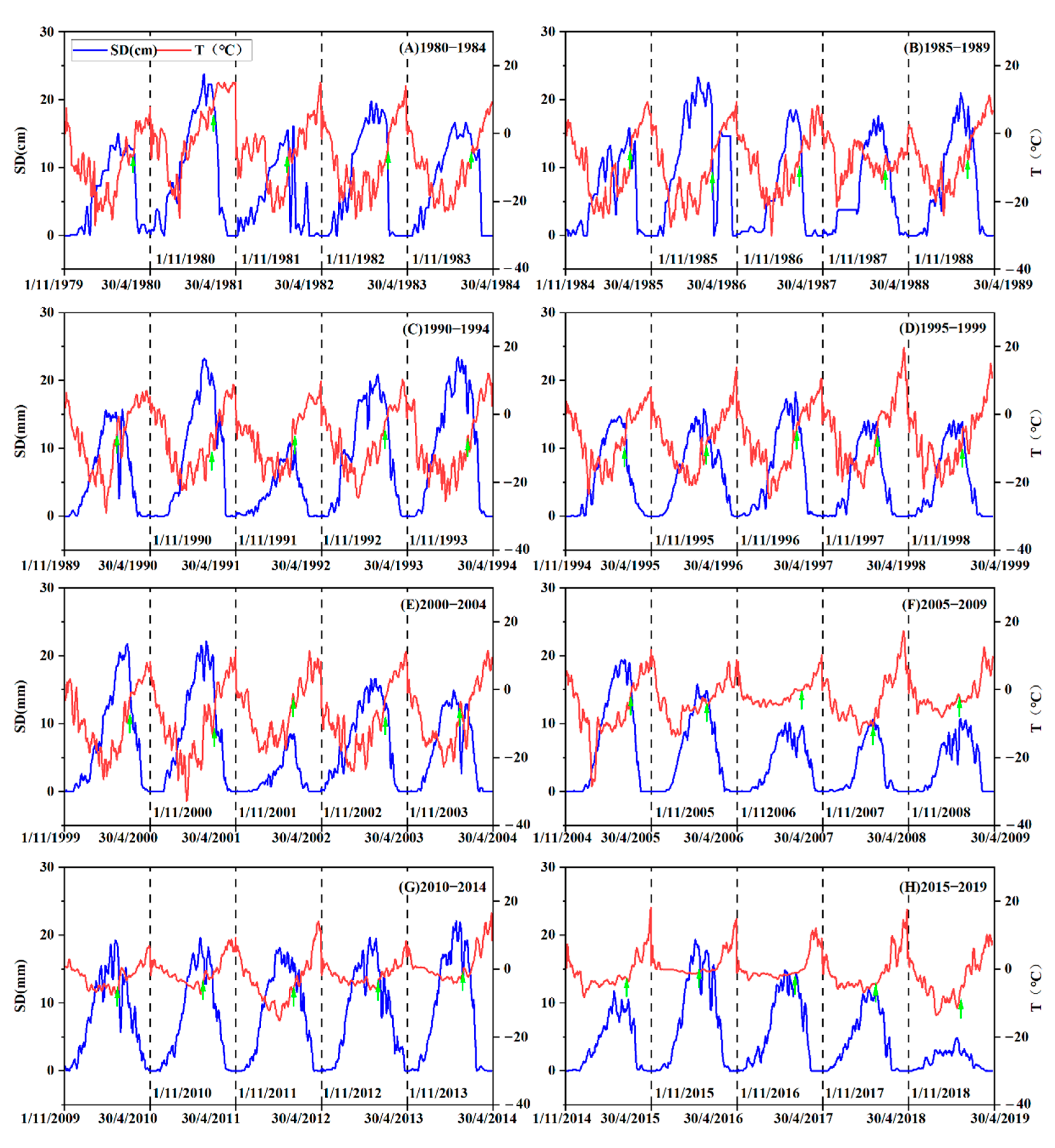
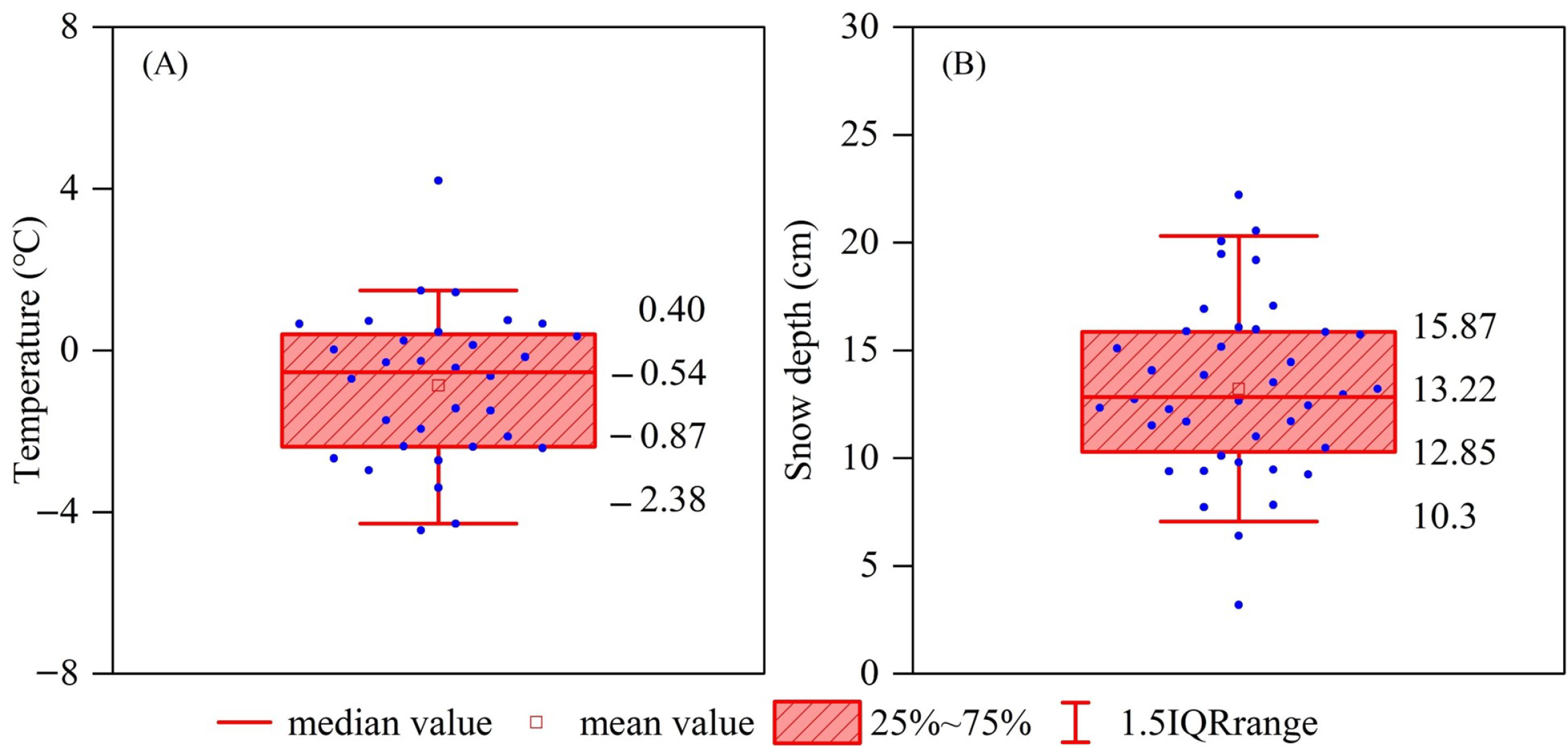
3.1.3. Snowmelt Temperature Threshold

The snowmelt temperature threshold is another critical parameter in the snowmelt calculation method described by Equation (2), which determines the time when snowmelt starts. In this study, we determine the value of this parameter by investigating the relationship between the 5-day moving averages of the snow depth and temperature from November to April in the next year. As shown in Figure 4, there is a clear negative correlation between the two quantities. In addition, the temperature from which the snow depth starts to fall sharply is determined as the snowmelt temperature threshold, as indicated by the green arrows.
The distribution of this parameter is plotted in Figure 5A, which shows that the snowmelt temperature threshold mainly concentrates around −2.38–0.40 °C from 1980 to 2019, with the annual average being −0.54 °C. Following this finding, we then modified the snowmelt temperature threshold in the model as −0.54 °C. The corresponding snow depth at the beginning of the snowmelt is 10.30–15.87cm (Figure 5B).

3.2. Setup and Validation of the Modified Model SWAT+

The setup of the modified model largely follows the same procedure of that for the original SWAT model, as the modifications are made only to the internal calculation components. Firstly, the DEM data (Figure 6A) were used to delineate the watersheds where the study area is divided into 31 watersheds (Figure 6B). Secondly, the hydrological response unit (HRU) is separated according to the terrain, land use, and soil types. Overall, there are 6 land use types (Figure 6C) and 17 soil types (Figure 6D). Before generating HRU, the spatial resolution of the land use, soil type, and DEM data is unified to 30 m × 30 m. In addition, the study area is classified into 227 HRUs. Finally, the meteorological data were imported and the initial model parameters were set.
The parameters of the model were then calibrated using the SUFI-2 algorithm provided by the standard Soil and Water Assessment Tool Calibration and Uncertainty Procedures (SWAT-CUP) component [70]. The SUFI-2 algorithm generates a group of parameters randomly by Latin-Hypercube simulations for seeking the best parameters combination [71]. In total, 28 parameters were chosen to be calibrated. The original range and fitted value of these parameters for both SWAT and SWAT+ are listed in Table 1.

3.3. Evaluation of the Modified Model SWAT+

We employed several indexes to compare the performance of SWAT+ against the original SWAT for snowmelt runoff simulation, including the root mean square error (RMSE), mean absolute error (MAE), relative error (RE), the coefficient of determination (R2), and Nash Sutcliffe coefficients (NSE) [72], as shown in Equations (7)–(11).
RMSE = i = 1 n ( R obs , i R mod , i ) 2 n
MAE = 1 n i = 1 n R obs , i R mod , i
RE = R mod , i R obs , i / R obs , i × 100 %
R 2 = i = 1 n R sim , i R sim ¯ R obs , i R obs ¯ 2 i = 1 n R sim , i R sim ¯ 2 i = 1 n R obs , i R obs ¯ 2
NSE = 1 i = 1 n ( R obs , i R mod , i ) 2 i = 1 n ( R obs , i R obs , i ¯ ) 2
where R obs , i and R mod , i are the observed snowmelt runoff and simulated snowmelt runoff and n is the total number of time steps (days) of the simulations.

3.4. Bias Correction Method for Climate Projection Data

The modified model SWAT+ was also used to simulate the climate change impact on future snowmelt runoff in the basin by coupling it with climate projections. Due to the limited spatial resolution, simplified physical processes, and incomplete understanding of the climate system, there are systematic deviations in the climate model projection data. As such, many bias correction methods have been developed and applied, e.g., delta method, multiple linear regressions, and quantile mapping [73,74,75]. In this study, we chose the delta method, which is widely used for climate projection data bias correction for its easy understanding and operation [76,77].
The delta method can eliminate the bias between climate scenario data and observations effectively [78]. We applied bias correction to two types of projection data inputs: precipitation and temperature. For precipitation, the correction is made using the variation ratio between the modeled precipitation and observed precipitation [79]. Similarly, temperature bias correction is based on the absolute variation between climate model temperature and observed temperature. The two correction methods are shown in Equations (12) and (13):
P adj = P ori × P obs P ori
T adj = T ori + T obs T ori
where P adj and P ori are the corrected and original precipitation of climate model data and P obs is observed precipitation;   T adj and T ori are the corrected and original temperature of climate model data. T obs is observed temperature.

4. Results

4.1. Model Performance Assessment

This section compares the SWAT+ model and the original SWAT model in terms of their performance for daily snowmelt runoff simulation in the study area. The results of the daily snowmelt runoff simulation (March–April) for the calibration period (1980–1999) and the validation period (2000–2019) are shown in Figure 7. It can be seen that, for low flow regimes, the snowmelt runoff is largely underestimated by the original SWAT model setting for both the calibration and validation periods, whereas the SWAT+ model performs better in this case.
The performances from the two models are further evaluated using the selected metrics and the results are shown in Table 2, which indicates a better performance of the SWAT+ model compared with the original SWAT model, showing improvements of MAE, RE, and RMSE by 20.56%, 93.12%, and 16.16%, respectively. In short, the snowmelt runoff simulation performance of the SWAT+ model is improved in comparison with the SWAT model, especially when the snowmelt runoff is small. This improvement in snowmelt runoff simulation underlines the benefits of the modification we made to the original SWAT model, i.e., adding total solar radiation in the SWAT model and localization of snowmelt temperature thresholds and snowmelt factors.

4.2. Projected Change in Snowmelt Runoff under Climate Change

Table 3 shows the projected precipitation and temperature during the snowmelt runoff period (March–April) from 2025 to 2054 and their corresponding changes relative to the baseline period (1980–2019). It appears that the Baishan basin will be warmer during 2025–2054 compared with the baseline period. Annual average temperature in 2025–2054 will increase by 2.53, 3.22, and 4.07 °C under the SSP2.6, SSP4.5, and SSP8.5 scenarios, respectively, compared with the baseline annual average temperature. In addition, the projected annual average precipitation will increase by 14.64% under SSP2.6, 9.29% under SSP4.5, and approximately 19.28% under SSP8.5.
The SWAT+ model was used to simulate the snowmelt runoff for both the baseline period (1980–2019) and the future (2025–2054) to assess the impact of climate change. For the baseline period, the simulation is driven by historical observations, whereas the future case is conducted using the projected forcing data, i.e., precipitation and temperature. As shown in Figure 8, the overall snowmelt runoff will reduce from March to April under the future climate scenarios compared with the baseline period. The annual average snowmelt runoff under SSP2.6, SSP4.5, and SSP8.5 is 148.3, 130.76, and 117.76 m3/s, with decreases of 31%, 39%, and 45%, respectively, from the baseline period (214.14 m3/s). The ensemble average of the snowmelt runoff presents clear and significant increase in March and a decrease in April, with peak flows shifting from April to March. This is due to the fact that snowmelt peak shifts to earlier spring as the temperature increases, causing significant increase in snowmelt runoff in March and a considerable decrease in April.

5. Discussion

5.1. Effect of the Modified Temperature Index Method

The traditional temperature index method in the SWAT model cannot represent the real snowmelt physical processes and leads to low simulation accuracy of snowmelt runoff. Therefore, some studies proposed to couple an energy balance model to the SWAT model to improve the low accuracy of snowmelt runoff simulation and reported good results [80,81]. However, other studies compared the performance of the improved temperature index model and the energy balance model and concluded that the improved temperature index model performed better than the energy balance model, with an extra benefit of requiring much less data [33,82]. In this study, we added the total solar radiation, which includes direct solar radiation and scattering solar radiation, to the traditional temperature index method, and further modifies the seasonal variation formula and determines the snowmelt temperature threshold. Compared with the SWAT model simulation results, the SWAT + decreased by 21.68% to 35.03% in MAE, RE, and RMSE metrics during calibration period. The NSE and the R2 indicators increased by 0.19 and 0.15, respectively. During the validation period, the MAE, RE, and RMSE indicators increased by 16.16% to 93.12%, while the NSE indicators and R2 indicators increased by 0.16 and 0.07.

5.2. Snowmelt Temperature Threshold

The 0 °C threshold used by the original SWAT model is only a rough indicator of snowmelt [83]. Some scholars noticed this problem and chose to use the accumulated temperature to determine whether the snowmelt has melted [84,85,86]. However, when calculating the accumulated temperature, snow melting below 0 °C is also ignored. This study determines the snowmelt temperature threshold by using the snow depth and temperature data from remote sensing. It helps mitigate the problem of poor availability of spatial and temporal coverage in snow observation data due to sparse distribution of snow measurement stations, especially in mountainous areas. The result shows that a better estimate of the temperature threshold of snowmelt in the Baishan watershed is around −0.54 °C, which is substantially lower than the prescribed 0 °C. This also confirms the results from some previous studies [87,88] and supports the argument that snow may melt when the temperature is well below 0 °C [89]. The reason is that there are many factors affecting snowmelt temperature threshold, such as impurities in the snow [90]. As such, snowmelt does not merely depend on the air temperature, it also depends on the balance of the energy fluxes, e.g., it can occur through solar heating when the air temperature is below 0 °C.

5.3. SWAT+ Model Uncertainty

Even though our results show the benefits of the SWAT+ model for snowmelt simulation in a seasonal snowmelt basin, we also recognize that the introduction of new variables will bring in extra uncertainty to the model. Studies on SWAT model uncertainty have been abundant in recent years; for example, the SUFI-2 algorithm and GLUE algorithm are widely used in the uncertainty analysis of the SWAT model [91,92]. This paper uses the SUFI-2 algorithm to judge the uncertainty of the SWAT+ model based on the criteria of the 95% prediction uncertainty (95 PPU) [93]. The 95 PPU has two characteristic indicators: P-factor and R-factor. P-factor is the percentage of observed data that are enveloped by 95 PPU and R-factor is the average thickness of 95 PPU. Larger P-factor and smaller R-factor indicate less model uncertainty. The simulation uncertainty is generally considered acceptable for P-factor > 0.7 and R-factor < 1 [94]. The P-factor of the SWAT + during the validation period was 0.86 and 0.67, respectively, and the R-factor was 0.92 and 0.77, respectively. It shows that the SWAT+ model uncertainty is acceptable.

5.4. Limitations and Further Studies

Our results show that the SWAT+ model uncertainty is acceptable. Further, there is also a certain amount of uncertainty in the process of determining the snowmelt threshold, snowmelt factor, as well as in the data derived from remote sensing, which needs to be fully examined and studied. The snow depth data used in this paper are derived from a passive microwave remote sensing data product. Although this product has been confirmed to have good applicability in Northeast China in general [61], its accuracy over the study area has not been extensively evaluated. At present, the accuracy evaluation of remote sensing data can be divided into two categories. One is the mutual verification conducted using observed data [95,96] and the other one can be mutually verified according to other types of remote sensing data [97,98]. Due to the lack of measured data, the future study will evaluate accuracy according to other types of remote sensing data. There are two ways to obtain multiple remote sensing snow depth data. One is to extract information about snow depth based on satellite remote sensing data by ourselves, for example, using a new algorithm to extract snow depth based on passive microwave measurements [99] or using relatively high spatial resolution active microwave measurements to capture the spatial variability of snow depth in a mountain area [100]. The other is to use ready-made remoting sensing snow depth data for accuracy evaluation, such as America National Snow and Ice Data Center AMSR-E data (http://nsidc.org/data/docs/daac/ae_swe_ease-grids.gd.html, accessed on 5 September 2022) and Japan Aerospace Exploration Agency AMSR2 data (https://suzaku.eorc.jaxa.jp/, accessed on 8 September 2022). Due to the limit of the scope of this study, the uncertainty quantification and representation of remote sensing data used in this paper are not included in this study. However, further work is planned to investigate the uncertainty associated with remote sensing data uncertainty [101,102].

6. Conclusions

SWAT model is a distributed hydrological model with a physical foundation and is widely used in hydrological simulations. The snowmelt module in the SWAT model adopts a relatively simple temperature index method together with assuming both the dates for maximum and minimum snowmelt factors and the snowmelt temperature threshold, which leads to underestimating snowmelt runoff obviously. This paper presents a study of improving snowmelt runoff simulation using SWAT by systematically addressing the issues mentioned above. Firstly, this study integrates the total solar radiation into the temperature index. Secondly, accurate dates of the maxima and minima of snowmelt factors are determined and snowmelt factor seasonal variation formulas are modified. Thirdly, the temperature threshold of snowmelt is determined by identifying the relationship between snow depth and temperature. Finally, the Baishan basin in Northeast China was selected to test SWAT+ model performance. The results show that SWAT+ performs better than the SWAT model in seasonal snowmelt zones, especially when the snowmelt runoff is in its low to medium range. In comparison with the SWAT model, the SWAT+ model has remarkable improvements in all selected performance metrics, i.e., MAE, RE, RMSE, R2, and NSE. Further, the effects of climate change on snowmelt runoff in the Baishan basin were investigated using the SWAT+ model. Compared with the baseline period (1980–2019), overall snowmelt runoff will reduce under SSP2.6, SSP4.5, and SSP8.5 scenarios. The annual average snowmelt runoff under SSP2.6, SSP4.5, and SSP8.5 are 148.3, 130.76, and 117.76 m3/s, a decrease of 31%, 39%, and 45%, respectively, from the baseline period (214.14 m3/s).

Author Contributions

Conceptualization, H.Z. and H.L.; methodology, H.Z.; software, C.L.; validation, H.Z., Y.X. and C.L.; formal analysis, H.Z.; investigation, Y.X.; resources, H.L.; data curation, H.N.; writing—original draft preparation, H.Z.; writing—review and editing, H.Z. and Y.X.; visualization, Y.X.; supervision, Y.X.; project administration, H.L.; funding acquisition, H.L. All authors have read and agreed to the published version of the manuscript.

Funding

This study was supported by Key Program of National Natural Science Foundation of China (42230204) and Key R&D project funding from Jilin Province Science and Technology Department, China (20200403070SF).

Institutional Review Board Statement

Not applicable.

Informed Consent Statement

Not applicable.

Data Availability Statement

The soil map and land use data are collected from the harmonized world soil database (version 1.1) (http://www.fao.org/soils-portal/data-hub/soil-maps-and-databases/harmonized-world-soil-database-v12, accessed on 25 December 2021) and resource and the environment science data center website (https://www.resdc.cn/, accessed on 15 January 2022), respectively. Daily precipitation, air temperature, wind speed, relative humidity, total solar radiation, and the snow depth discharge were obtained from the National Meteorological Science Data Center (https://data.cma.cn, accessed on 15 January 2022) and National Qinghai Tibet Plateau data center (http://data.tpdc.ac.cn, accessed on 5 April 2022). Climate projection data are from the Coupled Model Intercomparison Project (CMIP6) (http://cmip-pcmdi.llnl.gov/cmip6/, accessed on 3 July 2022).

Acknowledgments

The authors are thankful to State Grid Xinyuan Group Co., Lid Fengman Hydropower Station for help in data collection.

Conflicts of Interest

The authors declare no conflict of interest.

References

  1. Pangali Sharma, T.P.; Zhang, J.; Khanal, N.R.; Prodhan, F.A.; Paudel, B.; Shi, L.; Nepal, N. Assimilation of snowmelt runoff model (SRM) using satellite remote sensing data in Budhi Gandaki River Basin, Nepal. Remote Sens. 2020, 12, 1951. [Google Scholar] [CrossRef]
  2. Qi, W.; Feng, L.; Yang, H.; Liu, J. Spring and summer potential flood risk in Northeast China. J. Hydrol.-Reg. Stud. 2021, 38, 100951. [Google Scholar] [CrossRef]
  3. Tekeli, A.E.; Akyürek, Z.; Şorman, A.A.; Şensoy, A.; Şorman, A.Ü. Using MODIS snow cover maps in modeling snowmelt runoff process in the eastern part of Turkey. Remote Sens. Environ. 2005, 97, 216–230. [Google Scholar] [CrossRef]
  4. Nagler, T.; Rott, H.; Malcher, P.; Müller, F. Assimilation of meteorological and remote sensing data for snowmelt runoff forecasting. Remote Sens. Environ. 2008, 112, 1408–1420. [Google Scholar] [CrossRef]
  5. López-Moreno, J.I.; Pomeroy, J.W.; Alonso-González, E.; Morán-Tejeda, E.; Revuelto, J. Decoupling of warming mountain snowpacks from hydrological regimes. Environ. Res. Lett. 2020, 15, 114006. [Google Scholar] [CrossRef]
  6. Male, D.H.; Granger, R.J. Snow surface energy exchange. Water Resour. Res. 1981, 17, 609–627. [Google Scholar] [CrossRef]
  7. De Walle, D.R.; Rango, A. Principles of Snow Hydrology; Cambridge University Press: Cambridge, UK, 2008. [Google Scholar]
  8. Adhikari, T.R.; Talchabhadel, R.; Shrestha, S.; Sharma, S.; Aryal, D.; Pradhanang, S.M. The evaluation of climate change impact on hydrologic processes of a mountain river basin. Theor. Appl. Climatol. 2022, 150, 749–762. [Google Scholar] [CrossRef]
  9. Pandey, V.; Dhaubanjar, S.; Bharati, L.; Thapa, B. Spatio-temporal distribution of water availability in Karnali-Mohana Basin, Western Nepal: Climate change impact assessment (Part-B). J. Hydrol.-Reg. Stud. 2020, 29, 100691. [Google Scholar] [CrossRef]
  10. Seibert, J.; Bergström, S. A retrospective on hydrological catchment modelling based on half a century with the HBV model. Hydrol. Earth Syst. Sci. 2022, 26, 1371–1388. [Google Scholar] [CrossRef]
  11. Bergström, S. The HBV model. In Computer Models of Watershed Hydrology; Water Resources Publications: Littleton, CO, USA, 1995; pp. 443–476. [Google Scholar]
  12. Martinec, J.; Rango, A.; Roberts, R. Snowmelt Runoff Model (SRM) User’s Manual; Gómez-Landesa, E., Bleiweiss, M.P., Eds.; New Mexico State University: Las Cruces, NM, USA, 2008; p. 35. [Google Scholar]
  13. Xie, S.; Du, J.; Zhou, X.; Zhang, X.; Feng, X.; Zheng, W.; Li, Z.; Xu, C. A progressive segmented optimization algorithm for calibrating time-variant parameters of the snowmelt runoff model (SRM). J. Hydrol. 2018, 566, 470–483. [Google Scholar] [CrossRef]
  14. Quick, M.C.; Pipes, A. UBC WATERSHED MODEL/Le modèle du bassin versant UCB. Hydrol. Sci. J. 1977, 22, 153–161. [Google Scholar] [CrossRef]
  15. Adnan, M.; Liu, S.; Saifullah, M.; Iqbal, M.; Ali, A.F.; Mukhtar, M.A. Spatiotemporal variations in runoff and runoff components in response to climate change in a glacierized subbasin of the Upper Indus Basin, Pakistan. Front. Earth Sci. 2022, 10, 970349. [Google Scholar] [CrossRef]
  16. Fang, X.; Pomeroy, J.W. Diagnosis of future changes in hydrology for a Canadian Rockies headwater basin. Hydrol. Earth Syst. Sci. 2020, 24, 2731–2754. [Google Scholar] [CrossRef]
  17. Pomeroy, J.W.; Gray, D.M.; Brown, T.; Hedstrom, N.R.; Quinton, W.L.; Granger, R.J.; Carey, S.K. The cold regions hydrological model: A platform for basing process representation and model structure on physical evidence. Hydrol. Process. 2007, 21, 2650–2667. [Google Scholar] [CrossRef]
  18. Zhang, Z.; Kane, D.L.; Hinzman, L.D. Development and application of a spatially-distributed Arctic hydrological and thermal process model (ARHYTHM). Hydrol. Process. 2000, 14, 1017–1044. [Google Scholar] [CrossRef]
  19. Arnold, J.G.; Williams, J.R.; Srinivasan, R.; King, K.W. SWAT Manual; USDA Agricultural Service and Blackland Research Center: Temple, TX, USA, 1996. [Google Scholar]
  20. Tiwari, S.; Kar, S.C.; Bhatla, R.; Bansal, R. Temperature index based snowmelt runoff modelling for the Satluj River basin in the western Himalayas. Meteorol. Appl. 2018, 25, 302–313. [Google Scholar] [CrossRef]
  21. Pradhanang, S.M.; Anandhi, A.; Mukundan, R.; Zion, M.S.; Pierson, D.C.; Schneiderman, E.M.; Matonse, A.; Frei, A. Application of SWAT model to assess snowpack development and streamflow in the Cannonsville watershed, New York, USA. Hydrol. Process. 2011, 25, 3268–3277. [Google Scholar] [CrossRef]
  22. Siderius, C.; Biemans, H.; Wiltshire, A.; Rao, S.; Franssen, W.; Kumar, P.; Gosain, A.K.; Van Vliet, M.; Collins, D.N. Snowmelt contributions to discharge of the Ganges. Sci. Total Environ. 2013, 468, S93–S101. [Google Scholar] [CrossRef]
  23. Chiphang, N.; Bandyopadhyay, A.; Bhadra, A. Assessing the effects of snowmelt dynamics on streamflow and water balance components in an Eastern Himalayan river basin using SWAT model. Environ. Model. Assess. 2020, 25, 861–883. [Google Scholar] [CrossRef]
  24. Zhang, Y.; Liu, S. Progress of the application of degree-day model to study glaciers and snow cover. J. Glaciol Geocryol. 2006, 28, 101–107. [Google Scholar]
  25. Hock, R. Temperature index melt modelling in mountain areas. J. Hydrol. 2003, 282, 104–115. [Google Scholar] [CrossRef]
  26. Andrianaki, M.; Shrestha, J.; Kobierska, F.; Nikolaidis, N.P.; Bernasconi, S.M. Assessment of SWAT spatial and temporal transferability for a high-altitude glacierized catchment. Hydrol. Earth Syst. Sci. 2019, 23, 3219–3232. [Google Scholar] [CrossRef] [Green Version]
  27. Myers, D.T.; Ficklin, D.L.; Robeson, S.M. Incorporating rain-on-snow into the SWAT model results in more accurate simulations of hydrologic extremes. J. Hydrol. 2021, 603, 126972. [Google Scholar] [CrossRef]
  28. Qi, J.; Li, S.; Jamieson, R.; Hebb, D.; Xing, Z.; Meng, F. Modifying SWAT with an energy balance module to simulate snowmelt for maritime regions. Environ. Modell. Softw. 2017, 93, 146–160. [Google Scholar] [CrossRef]
  29. Debele, B.; Srinivasan, R.; Gosain, A.K. Comparison of Process-Based and Temperature-Index Snowmelt Modeling in SWAT. Water Resour. Manag. 2010, 24, 1065–1088. [Google Scholar] [CrossRef]
  30. Meng, X.; Ji, X.; Liu, Z.; Xiao, J.; Chen, X.; Wang, F. Research on improvement and application of snowmelt module in SWAT. J. Nat. Resour. 2014, 29, 528–539. [Google Scholar]
  31. Pellicciotti, F.; Brock, B.; Strasser, U.; Burlando, P.; Funk, M.; Corripio, J. An enhanced temperature-index glacier melt model including the shortwave radiation balance: Development and testing for Haut Glacier d’Arolla, Switzerland. J. Glaciol. 2005, 51, 573–587. [Google Scholar] [CrossRef]
  32. Irvine Fynn, T.D.; Hanna, E.; Barrand, N.E.; Porter, P.R.; Kohler, J.; Hodson, A.J. Examination of a physically based, high-resolution, distributed Arctic temperature-index melt model, on Midtre Lovénbreen, Svalbard. Hydrol. Process. 2014, 28, 134–149. [Google Scholar] [CrossRef]
  33. Shakoor, A.; Burri, A.; Bavay, M.; Ejaz, N.; Ghumman, A.R.; Comola, F.; Lehning, M. Hydrological response of two high altitude Swiss catchments to energy balance and temperature index melt schemes. Polar Sci. 2018, 17, 1–12. [Google Scholar] [CrossRef]
  34. Painter, T.H.; Skiles, S.M.; Deems, J.S.; Brandt, W.T.; Dozier, J. Variation in Rising Limb of Colorado River Snowmelt Runoff Hydrograph Controlled by Dust Radiative Forcing in Snow. Geophys. Res. Lett. 2017, 45, 797–808. [Google Scholar] [CrossRef] [Green Version]
  35. Ohmura, A. Physical basis for the temperature-based melt-index method. J. Appl. Meteorol. 2001, 40, 753–761. [Google Scholar] [CrossRef]
  36. Bouamri, H.; Boudhar, A.; Gascoin, S.; Kinnard, C. Performance of temperature and radiation index models for point-scale snow water equivalent (SWE) simulations in the Moroccan High Atlas Mountains. Hydrol. Sci. J. 2018, 63, 1844–1862. [Google Scholar] [CrossRef]
  37. Meriö, L. The Measurement and Modeling of Snowmelt in Sub-Arctic Site Using Low Cost Temperature Loggers. Master’s Thesis, University of Oulu, Oulu, Finland, 2015. [Google Scholar]
  38. Singh, V.; Jain, S.K.; Goyal, M.K. An assessment of snow-glacier melt runoff under climate change scenarios in the Himalayan basin. Stoch. Environ. Res. Risk Assess. 2021, 35, 2067–2092. [Google Scholar] [CrossRef]
  39. Dombrovsky, L.A.; Kokhanovsky, A.A.; Randrianalisoa, J.H. On snowpack heating by solar radiation: A computational model. J. Quant. Spectrosc. Radiat. Transf. 2019, 227, 72–85. [Google Scholar] [CrossRef]
  40. Martinec, J.; Rango, A. Parameter values for snowmelt runoff modelling. J. Hydrol. 1986, 84, 197–219. [Google Scholar] [CrossRef]
  41. Neitsch, S.L.; Arnold, J.G.; Kiniry, J.R.; Williams, J.R. Soil and Water Assessment Tool Theoretical Documentation Version 2009; Texas Water Resources Institute: College Station, TX, USA, 2011. [Google Scholar]
  42. Li, H.; Li, X.; Yang, D.; Wang, J.; Gao, B.; Pan, X.; Zhang, Y.; Hao, X. Tracing snowmelt paths in an integrated hydrological model for understanding seasonal snowmelt contribution at basin scale. J. Geophys. Res.-Atmos. 2019, 124, 8874–8895. [Google Scholar] [CrossRef]
  43. Tang, J.; Liu, G.; Xie, Y.; Dun, X.; Wang, D.; Zhang, S. Ephemeral gullies caused by snowmelt: A ten-year study in northeastern China. Soil Tillage Res. 2021, 212, 105048. [Google Scholar] [CrossRef]
  44. Musselman, K.N.; Clark, M.P.; Liu, C.; Ikeda, K.; Rasmussen, R. Slower snowmelt in a warmer world. Nat. Clim. Chang. 2017, 7, 214–219. [Google Scholar] [CrossRef]
  45. Wu, X.; Che, T.; Li, X.; Wang, N.; Yang, X. Slower Snowmelt in Spring Along With Climate Warming across the Northern Hemisphere. Geophys. Res. Lett. 2018, 45, 12, 312–331, 339. [Google Scholar] [CrossRef]
  46. Liu, Y.; Cui, G.; Li, H. Optimization and Application of Snow Melting Modules in SWAT Model for the Alpine Regions of Northern China. Water 2020, 12, 636. [Google Scholar] [CrossRef] [Green Version]
  47. Blahušiaková, A.; Matoušková, M.; Jeníček, M.; Ledvinka, O.; Kliment, Z.; Podolinská, J.; Snopková, Z. Snow and climate trends and their impact on seasonal runoff and hydrological drought types in selected mountain catchments in Central Europe. Hydrol. Sci. J. 2020, 65, 2083–2096. [Google Scholar] [CrossRef]
  48. Godsey, S.E.; Kirchner, J.W.; Tague, C.L. Effects of changes in winter snowpacks on summer low flows: Case studies in the Sierra Nevada, California, USA. Hydrol. Process. 2014, 28, 5048–5064. [Google Scholar] [CrossRef]
  49. Kaplan, H. Algorithm Theory: SWAT 2010; Springer: Berlin/Heidelberg, Germany, 2010. [Google Scholar]
  50. Duan, Y.; Luo, M.; Guo, X.; Cai, P.; Li, F. Study on the Relationship between Snowmelt Runoff for Different Latitudes and Vegetation Growth Based on an Improved SWAT Model in Xinjiang, China. Sustainability 2021, 13, 1189. [Google Scholar] [CrossRef]
  51. Uwamahoro, S.; Liu, T.; Nzabarinda, V.; Habumugisha, J.M.; Habumugisha, T.; Harerimana, B.; Bao, A. Modifications to Snow-Melting and Flooding Processes in the Hydrological Model—A Case Study in Issyk-Kul, Kyrgyzstan. Atmosphere 2021, 12, 1580. [Google Scholar] [CrossRef]
  52. Kuhn, M. Micro-meteorological conditions for snow melt. J. Glaciol. 1987, 33, 24–26. [Google Scholar] [CrossRef] [Green Version]
  53. Zhang, W.; Shen, Y.; He, J. Snow properties on different underlying surfaces during snow-melting period in the Altay Mountains: Observation and analysis. J. Glaciol. Geocryol. 2014, 36, 491–499. [Google Scholar]
  54. Vorkauf, M.; Marty, C.; Kahmen, A.; Hiltbrunner, E. Past and future snowmelt trends in the Swiss Alps: The role of temperature and snowpack. Clim. Chang. 2021, 165, 44. [Google Scholar] [CrossRef]
  55. Li, W.; Cidan, Y.; Wang, A.; Li, H.; Tian, L. Identification of influencing factors and machanism of spring runoff in Baishan Watershed, China. Water Resour. Hydropower Eng. 2019, 50, 63–72. [Google Scholar]
  56. Che, T.; Li, X.; Jin, R.; Armstrong, R.; Zhang, T. Snow depth derived from passive microwave remote-sensing data in China. Ann. Glaciol. 2008, 49, 145–154. [Google Scholar] [CrossRef] [Green Version]
  57. Dai, L.; Che, T.; Ding, Y. Inter-calibrating SMMR, SSM/I and SSMI/S data to improve the consistency of snow-depth products in China. Remote Sens. 2015, 7, 7212–7230. [Google Scholar] [CrossRef] [Green Version]
  58. Liu, Y.; Xu, J.; Lu, X.; Nie, L. Assessment of glacier-and snowmelt-driven streamflow in the arid middle Tianshan Mountains of China. Hydrol. Process. 2020, 34, 2750–2762. [Google Scholar] [CrossRef]
  59. Wu, X.; Wang, X.; Liu, S.; Yang, Y.; Xu, G.; Xu, Y.; Jiang, T.; Xiao, C. Snow cover loss compounding the future economic vulnerability of western China. Sci. Total Environ. 2021, 755, 143025. [Google Scholar] [CrossRef] [PubMed]
  60. Zhu, L.; Zhang, Y.; Wang, J.; Tian, W.; Liu, Q.; Ma, G.; Kan, X.; Chu, Y. Downscaling Snow Depth Mapping by Fusion of Microwave and Optical Remote-Sensing Data Based on Deep Learning. Remote Sens. 2021, 13, 584. [Google Scholar] [CrossRef]
  61. Yang, Y.; Chen, R.; Liu, G.; Liu, Z.; Wang, X. Trends and variability in snowmelt in China under climate change. Hydrol. Earth Syst. Sci. 2022, 26, 305–329. [Google Scholar] [CrossRef]
  62. Wang, Q.; Zhai, P. CMIP6 Projections of the “Warming-Wetting” Trend in Northwest China and Related Extreme Events Based on Observational Constraints. J. Meteorol. Res. 2022, 36, 239–250. [Google Scholar] [CrossRef]
  63. Meier, H.M.; Kniebusch, M.; Dieterich, C.; Gröger, M.; Zorita, E.; Elmgren, R.; Myrberg, K.; Ahola, M.P.; Bartosova, A.; Bonsdorff, E. Climate change in the Baltic Sea region: A summary. Earth Syst. Dynam. 2022, 13, 457–593. [Google Scholar] [CrossRef]
  64. Collados-Lara, A.; Pardo-Igúzquiza, E.; Pulido-Velazquez, D. A distributed cellular automata model to simulate potential future impacts of climate change on snow cover area. Adv. Water Resour. 2019, 124, 106–119. [Google Scholar] [CrossRef]
  65. Herbert, L. Relations between glacier runoff and meteorological factors observed on and outside the glacier. In International Association of Scientific Hydrology: Commission of Snow and Ice. Reports and Discussion. Rapports Et Discussions; University of Michigan: Ann Arbor, MI, USA, 1968; p. 429. [Google Scholar]
  66. Zuzel, J.F.; Cox, L.M. Relative importance of meteorological variables in snowmelt. Water Resour. Res. 1975, 11, 174–176. [Google Scholar] [CrossRef]
  67. Liu, H.; Xiao, P.; Zhang, X. The characteristics of snow cover albedo in Northeast China. J. Glaciol. Geocryol. 2019, 41, 554–562. [Google Scholar]
  68. Fontaine, T.A.; Cruickshank, T.S.; Arnold, J.G.; Hotchkiss, R.H. Development of a snowfall–Snowmelt routine for mountainous terrain for the soil water assessment tool (SWAT). J. Hydrol. 2002, 262, 209–223. [Google Scholar] [CrossRef]
  69. Anderson, E.A. Development and testing of snow pack energy balance equations. Water Resour. Res. 1968, 4, 19–37. [Google Scholar] [CrossRef]
  70. Abbaspour, K.C.; Vejdani, M.; Haghighat, S.; Yang, J. SWAT-CUP Calibration and Uncertainty Programs for SWAT; Swiss Federal Institute of Aquatic Science and Technology: Dübendorf, Switzerland, 2007; pp. 1596–1602. [Google Scholar]
  71. Abbaspour, K.C.; Johnson, C.A.; Van Genuchten, M.T. Estimating uncertain flow and transport parameters using a sequential uncertainty fitting procedure. Vadose Zone J. 2004, 3, 1340–1352. [Google Scholar] [CrossRef]
  72. Nash, J.E.; Sutcliffe, J.V. River flow forecasting through conceptual models part I—A discussion of principles. J. Hydrol. 1970, 10, 282–290. [Google Scholar] [CrossRef]
  73. Maraun, D. Bias correction, quantile mapping, and downscaling: Revisiting the inflation issue. J. Clim. 2013, 26, 2137–2143. [Google Scholar] [CrossRef] [Green Version]
  74. Durai, V.R.; Bhradwaj, R. Evaluation of statistical bias correction methods for numerical weather prediction model forecasts of maximum and minimum temperatures. Nat. Hazards 2014, 73, 1229–1254. [Google Scholar] [CrossRef]
  75. Räty, O.; Räisänen, J.; Ylhäisi, J.S. Evaluation of delta change and bias correction methods for future daily precipitation: Intermodel cross-validation using ENSEMBLES simulations. Clim. Dynam. 2014, 42, 2287–2303. [Google Scholar] [CrossRef]
  76. Navarro-Racines, C.; Tarapues, J.; Thornton, P.; Jarvis, A.; Ramirez-Villegas, J. High-resolution and bias-corrected CMIP5 projections for climate change impact assessments. Sci. Data 2020, 7, 7. [Google Scholar] [CrossRef] [PubMed] [Green Version]
  77. Xavier, A.C.F.; Martins, L.L.; Rudke, A.P.; de Morais, M.V.B.; Martins, J.A.; Blain, G.C. Evaluation of Quantile Delta Mapping as a bias-correction method in maximum rainfall dataset from downscaled models in São Paulo state (Brazil). Int. J. Climatol. 2022, 42, 175–190. [Google Scholar] [CrossRef]
  78. Su, F.; Zhang, L.; Ou, T.; Chen, D.; Yao, T.; Tong, K.; Qi, Y. Hydrological response to future climate changes for the major upstream river basins in the Tibetan Plateau. Glob. Planet. Chang. 2016, 136, 82–95. [Google Scholar] [CrossRef]
  79. Hay, L.E.; Wilby, R.L.; Leavesley, G.H. A comparison of delta change and downscaled GCM scenarios for three mountainous basins in the United States 1. J. Am. Water Resour. Assoc. 2000, 36, 387–397. [Google Scholar] [CrossRef]
  80. Meng, X.; Yu, D.; Liu, Z. Energy balance-based SWAT model to simulate the mountain snowmelt and runoff—Taking the application in Juntanghu watershed (China) as an example. J. Mt. Sci.-Engl. 2015, 12, 368–381. [Google Scholar] [CrossRef]
  81. Qi, J.; Li, S.; Li, Q.; Xing, Z.; Bourque, C.P.; Meng, F. Assessing an enhanced version of SWAT on water quantity and quality simulation in regions with seasonal snow cover. Water Resour. Manag. 2016, 30, 5021–5037. [Google Scholar] [CrossRef]
  82. Kustas, W.P.; Rango, A.; Uijlenhoet, R. A simple energy budget algorithm for the snowmelt runoff model. Water Resour. Res. 1994, 30, 1515–1527. [Google Scholar] [CrossRef]
  83. Green, R.O.; Painter, T.H.; Roberts, D.A.; Dozier, J. Measuring the expressed abundance of the three phases of water with an imaging spectrometer over melting snow. Water Resour. Res. 2006, 42. [Google Scholar] [CrossRef]
  84. Duan, Y.; Meng, F.; Liu, T.; Huang, Y.; Luo, M.; Xing, W.; De Maeyer, P. Sub-Daily Simulation of Mountain Flood Processes Based on the Modified Soil Water Assessment Tool (SWAT) Model. Int. J. Environ. Res. Public Health 2019, 16, 3118. [Google Scholar] [CrossRef]
  85. Duan, Y.; Liu, T.; Meng, F.; Luo, M.; Frankl, A.; De Maeyer, P.; Bao, A.; Kurban, A.; Feng, X. Inclusion of Modified Snow Melting and Flood Processes in the SWAT Model. Water 2018, 10, 1715. [Google Scholar] [CrossRef] [Green Version]
  86. Duan, Y.; Liu, T.; Meng, F.; Yuan, Y.; Luo, M.; Huang, Y.; Xing, W.; Nzabarinda, V.; De Maeyer, P. Accurate Simulation of Ice and Snow Runoff for the Mountainous Terrain of the Kunlun Mountains, China. Remote Sens. 2020, 12, 179. [Google Scholar] [CrossRef] [Green Version]
  87. Brubaker, K.; Rango, A.; Kustas, W. Incorporating radiation inputs into the snowmelt runoff model. Hydrol. Process. 1996, 10, 1329–1343. [Google Scholar] [CrossRef]
  88. Mohammed, A.A.; Pavlovskii, I.; Cey, E.E.; Hayashi, M. Effects of preferential flow on snowmelt partitioning and groundwater recharge in frozen soils. Hydrol. Earth Syst. Sci. 2019, 23, 5017–5031. [Google Scholar] [CrossRef] [Green Version]
  89. Kuipers Munneke, P.; Van den Broeke, M.R.; King, J.C.; Gray, T.; Reijmer, C.H. Near-surface climate and surface energy budget of Larsen C ice shelf, Antarctic Peninsula. Cryosphere 2012, 6, 353–363. [Google Scholar] [CrossRef] [Green Version]
  90. Jones, H.; Pomeroy, J.; Walker, D.; Hoham, R. Snow Ecology; Cambridge University Press: Cambridge, UK, 2001. [Google Scholar]
  91. Yesuf, H.M.; Melesse, A.M.; Zeleke, G.; Alamirew, T. Streamflow prediction uncertainty analysis and verification of SWAT model in a tropical watershed. Environ. Earth Sci. 2016, 75, 806. [Google Scholar] [CrossRef]
  92. Abbas, T.; Hussain, F.; Nabi, G.; Boota, M.; Wu, R. Uncertainty evaluation of SWAT model for snowmelt runoff in a Himalayan watershed. Terr. Atmos. Ocean. Sci. 2019, 30, 1–15. [Google Scholar] [CrossRef] [Green Version]
  93. Khalid, K.; Ali, M.F.; Rahman, N.F.A.; Mispan, M.R.; Haron, S.H.; Othman, Z.; Bachok, M.F. Sensitivity Analysis in Watershed Model Using SUFI-2 Algorithm. Procedia Eng. 2016, 162, 441–447. [Google Scholar] [CrossRef] [Green Version]
  94. Mengistu, A.G.; van Rensburg, L.D.; Woyessa, Y.E. Techniques for calibration and validation of SWAT model in data scarce arid and semi-arid catchments in South Africa. J. Hydrol.-Reg. Stud. 2019, 25, 100621. [Google Scholar] [CrossRef]
  95. Dai, L.; Che, T.; Wang, J.; Zhang, P. Snow depth and snow water equivalent estimation from AMSR-E data based on a priori snow characteristics in Xinjiang, China. Remote Sens. Environ. 2012, 127, 14–29. [Google Scholar] [CrossRef]
  96. Yang, X.; Zheng, Z.; Yang, Z. Validation of AMSR-E snow depth products in Inner Mongolia. Remote Sens. Appl. 2011, 6, 61–68. [Google Scholar]
  97. Liu, J.; Li, Z.; Huang, L.; Tian, B. Hemispheric-scale comparison of monthly passive microwave snow water equivalent products. J. Appl. Remote Sens. 2014, 8, 84688. [Google Scholar] [CrossRef] [Green Version]
  98. Che, T.; Li, X.; Gao, F. Estimation of snow water equivalent in the Tibetan Plateau using passive microwave remote sensing data (SSM/I). J. Glaciol. Geocryol. 2004, 26, 363–368. [Google Scholar]
  99. Li, D.; Durand, M.; Margulis, S. Potential for hydrologic monitoring of deep mountain snowpack via passive microwave remote sensing: Kern River basin, Sierra Nevada, USA. Remote Sens. Environ. 2010, 125, 34–48. [Google Scholar] [CrossRef]
  100. Lievens, H.; Demuzere, M.; Marshall, H.; Reichle, R.H.; Brucker, L.; Brangers, I.; de Rosnay, P.; Dumont, M.; Girotto, M.; Immerzeel, W.W.; et al. Snow depth variability in the Northern Hemisphere mountains observed from space. Nat. Commun. 2019, 10, 4629. [Google Scholar] [CrossRef] [Green Version]
  101. Hiemstra, C.A.; Liston, G.E.; Reiners, W.A. Snow Redistribution by Wind and Interactions with Vegetation at Upper Treeline in the Medicine Bow Mountains, Wyoming, USA. Arct. Antarct. Alp. Res. 2002, 34, 262–273. [Google Scholar] [CrossRef]
  102. Egli, L.; Jonas, T. Hysteretic dynamics of seasonal snow depth distribution in the Swiss Alps. Geophys. Res. Lett. 2009, 36, L02501. [Google Scholar] [CrossRef]
Figure 1. Map of the Baishan basin location, river networks, gauging station, and weather stations.
Remotesensing 14 05823 g001
Figure 2. (AH) Relationship between solar radiation (SR) and snow depth (SD) from November to April in the year after during 1980–2019. The black arrows indicate the time when the minimum snowmelt factor occurs. The green arrows indicate the time when the maximum snowmelt factor occurs.
Remotesensing 14 05823 g002
Figure 3. Dates of the minimum snowmelt factor (A) and maximum snowmelt factor (B).
Remotesensing 14 05823 g003
Figure 4. (AH) Relationship between snow depth (SD (cm)) and temperature (T (°C)) of November to April in the next year during 1980–2019. Green arrows indicate the snowmelt temperature threshold.
Remotesensing 14 05823 g004
Figure 5. Snowmelt temperature threshold (A) and snow depth at the beginning of the snowmelt (B) from 1980 to 2019. Blue dots indicate annual data point.
Remotesensing 14 05823 g005
Figure 6. SWAT model setup: (A) DEM, (B) watershed, (C) land use, (D) soil type.
Remotesensing 14 05823 g006
Figure 7. Snowmelt runoff simulations from March to April during calibration period (A) and validation period (B) of SWAT model and SWAT+ model.
Remotesensing 14 05823 g007
Figure 8. Annual average snowmelt runoff during 1980–2019 and 2020–2045 under SSP 2.6, SSP 4.5, and SSP 8.5 climate change scenarios, respectively.
Remotesensing 14 05823 g008
Table 1. Parameters for SWAT and SWAT+.
Parameter
Name
MeaningMaxMinSWAT Fitted
Value
SWAT+ Fitted
Value
SFTMPSnowfall temperature (°C)5−50.82−0.07
ESCOSoil evaporation compensation factor10.010.300.65
EPCOPlant uptake compensation factor10.010.980.09
CN2SCS runoff curve number for moisture condition II0.5−0.50.290.52
BIOMIXBiological mixing efficient0.5−0.50.92−0.21
SOL_ZDepth from soil surface to bottom of layer (mm)0.5−0.50.22−0.13
SOL_AWCAvailable water capacity of the soil layer
(mm H2O/mm soil)
0.5−0.50.680.64
SOL_KSaturated hydraulic conductivity (mm/h)0.8−0.81.130.09
SOL_ALBMoist soil albedo0.5−0.50.01−0.09
GW_DELAYGroundwater delay time (days)5000431.71111.34
ALPHA_BFBaseflow Alpha Factor101.690.47
SMTMPSnow melt base temperature (°C)5−50.00−1.46
GWQMNThreshold depth of water in the shallow aquifer required for return flow to occur
(mm H2O)
500001380.817057.22
GW_REVAPGroundwater “revap” coefficient0.20.020.190.12
REVAPMNThreshold depth of water in the shallow aquifer for “revap” or percolation to the deep aquifer to occur (mm H2O)5000106.88−21.94
CH_N2Manning’s “n” value for the main channel0.300.150.35
CH_K2Effective hydraulic conductivity in main channel alluvium (mm/h)1500145.12−46.50
RCHRG_DPDeep aquifer percolation fraction100.950.42
SMFMXMelt factor for snow on 21 June
(mm H2O/°C-day)
1000.367.73
SMFMNMelt factor for snow on 21 Dec
(mm H2O/°C-day)
1000.586.31
TIMPSnow pack temperature lag factor10.010.500.13
SURLAGSurface runoff lag coefficient2414.935.88
TLAPSTemperature lapse rate (°C/km)10−104.80−1.95
SLSUBBSNAverage slope length (m)15010−7.7415.78
CANMXMaximum canopy storage (mm H2O)1000−2.37−11.74
Table 2. Snowmelt runoff simulation accuracy of SWAT model and SWAT+ model.
MetricsCalibrationValidation
SWATSWAT+ChangeSWATSWAT+Change
MAE98.6677.27−21.68%106.9884.99−20.56%
RE−32.09−20.85−35.03%−343.90−23.67−93.12%
RMSE155.76117.41−24.62%144.39121.05−16.16%
NSE0.550.740.190.470.630.16
R20.630.780.150.630.700.07
Table 3. Precipitation (P) and temperature (T) during the snowmelt runoff period from 2025 to 2054.
BaselineSSP2.6SSP4.6SSP8.5
ProjectionsChangeProjectionsChangeProjectionsChange
T1.05 °C2.53 °C1.48 °C3.22 °C2.17 °C4.07 °C3.02 °C
P66.14 mm75.82 mm14.64%72.29 mm9.29%78.89 mm19.28%
Publisher’s Note: MDPI stays neutral with regard to jurisdictional claims in published maps and institutional affiliations.

