
Reconstruction of Near-Surface Air Temperature over the Greenland Ice Sheet Based on MODIS Data and Machine Learning Approaches
 , , , and
Abstract
:1. Introduction
2. Data and Methods
2.1. Data
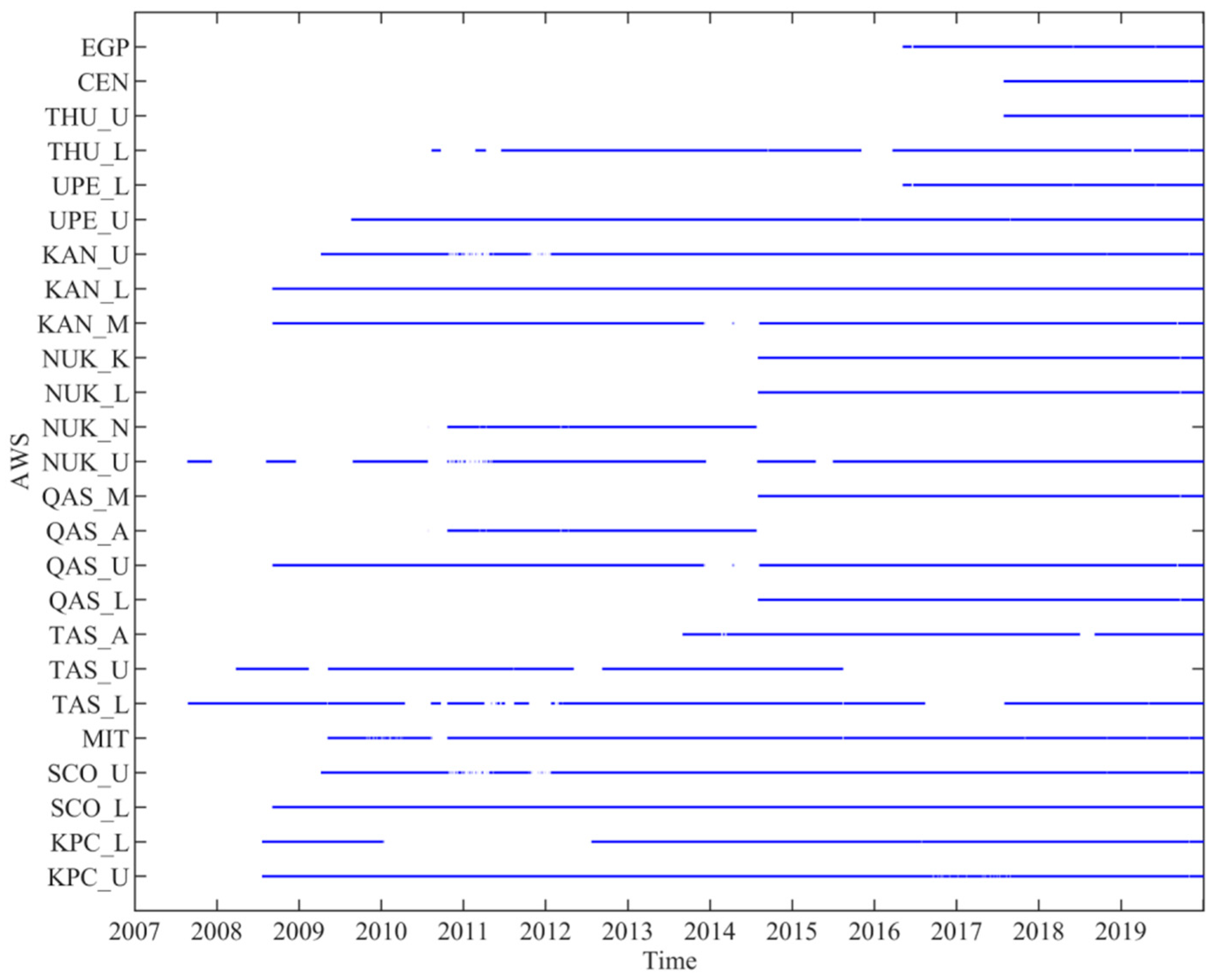
2.1.1. In Situ Data
2.1.2. Satellite Data
2.1.3. Regional Climate Model
2.2. Methods
2.2.1. Machine Learning
- (1)
- Neural network (NN)
- (2)
- Gaussian process regression (GPR)
- (3)
- Support vector machine (SVM)
- (4)
- Random forest (RF)
2.2.2. Factor Determination
- (1)
- Daily data factor determination
- (2)
- Monthly data factor determination
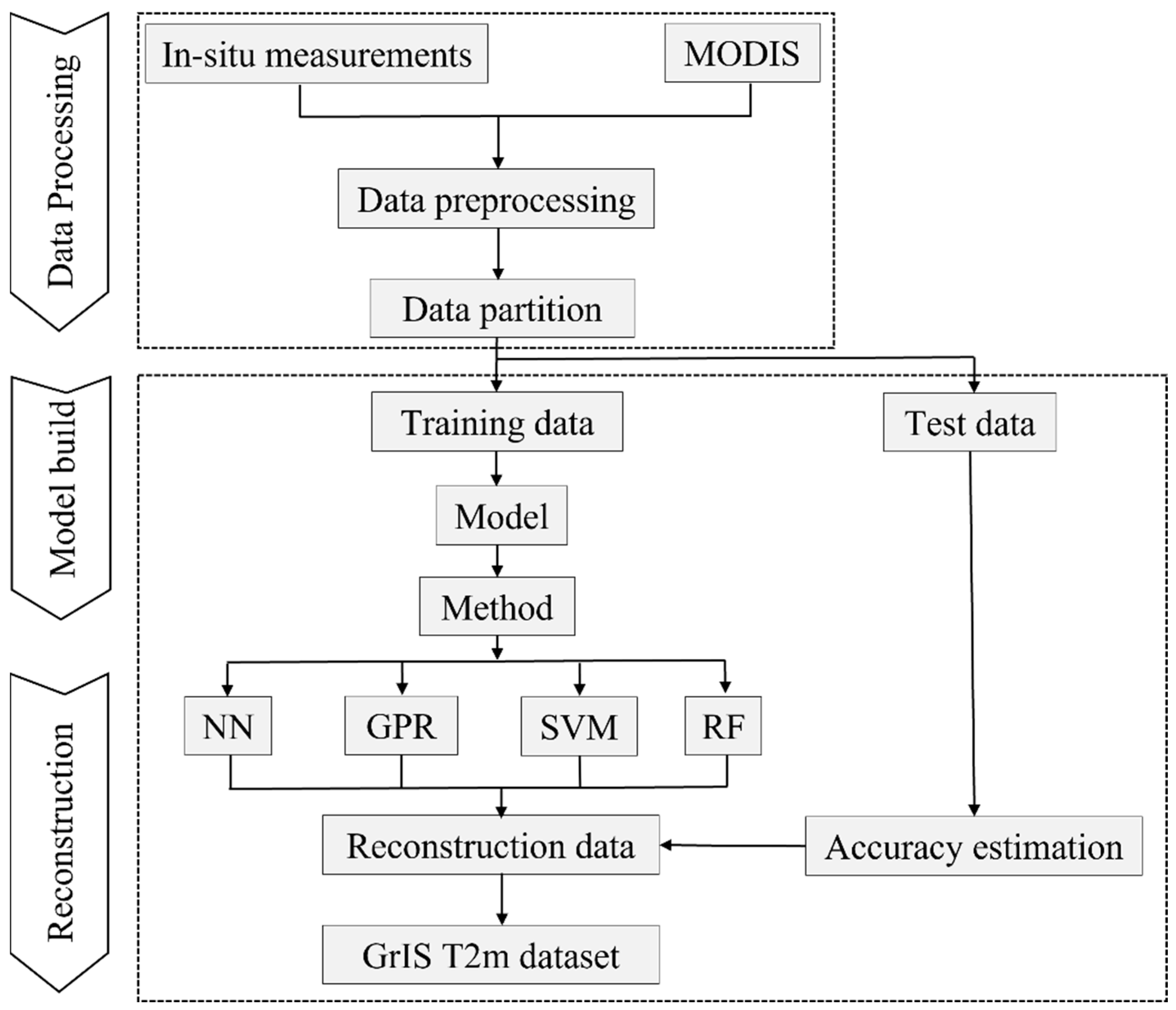
2.2.3. Feature Ranking and Model Construction
- (1)
- Establishment of the daily data model
- (2)
- Establishment of the monthly data model
3. Results
3.1. Daily Data Reconstruction Products
3.2. Monthly Data Reconstruction Products
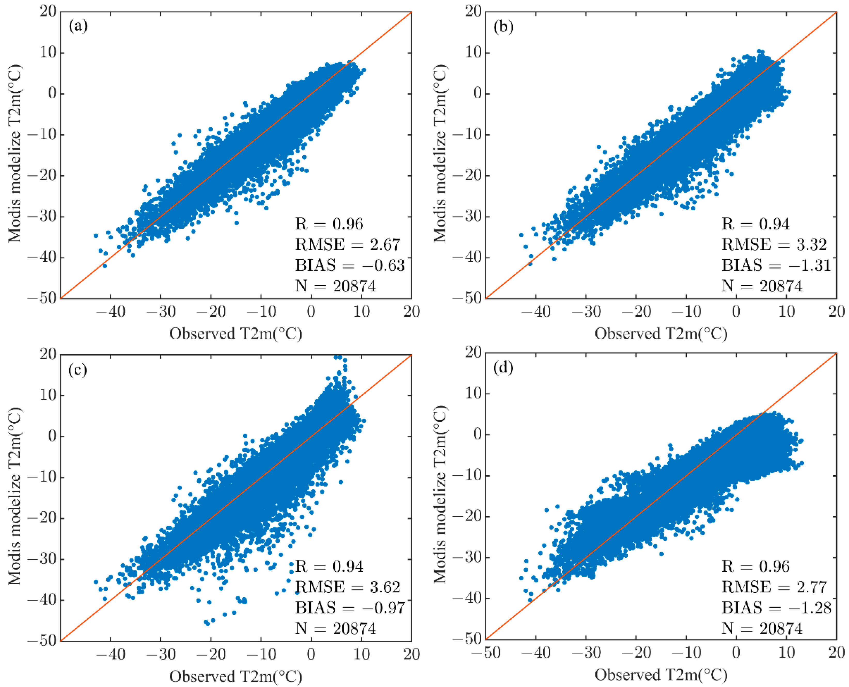
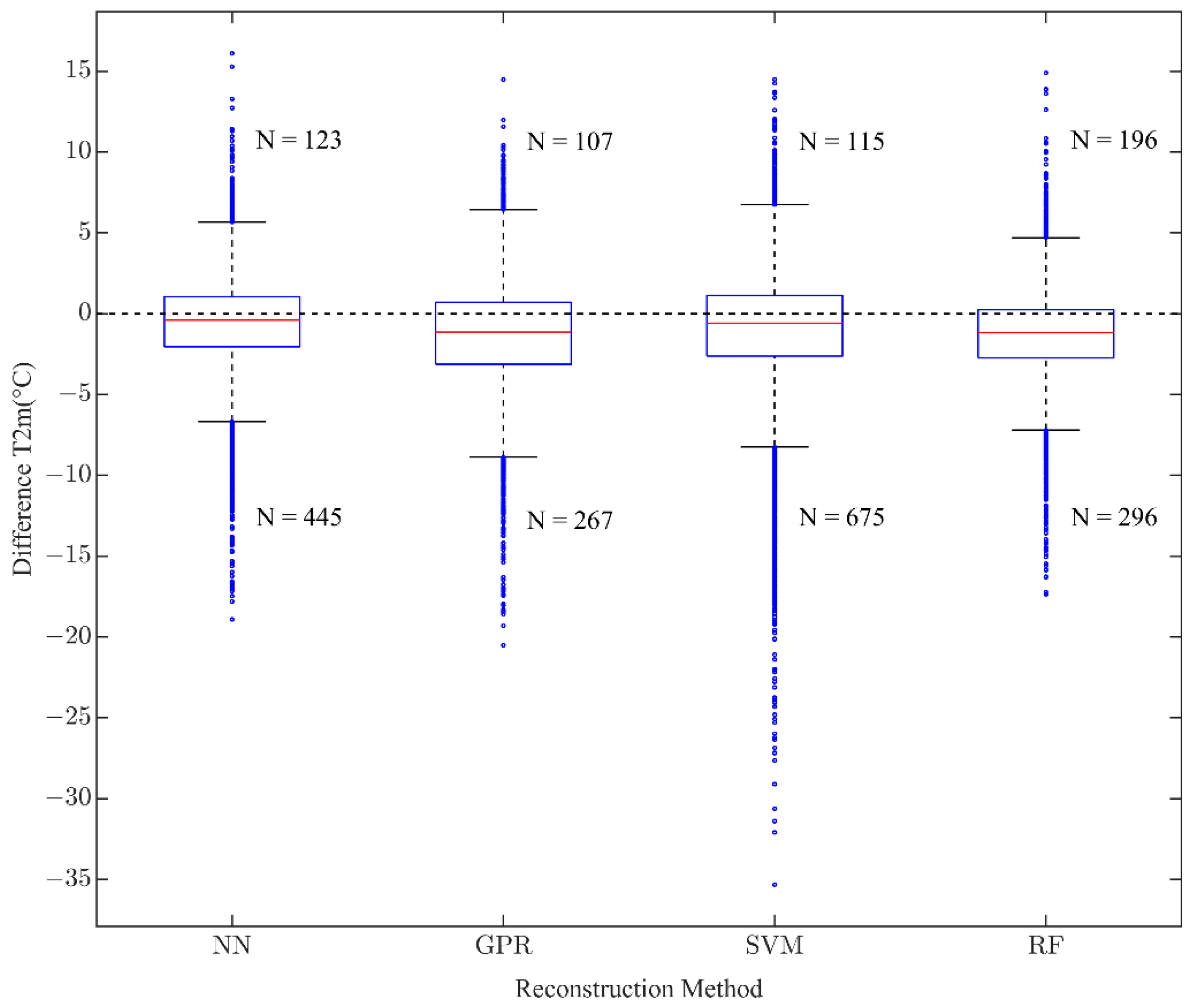
3.3. Evaluation of the Reconstruction Products Performance
4. Discussion
4.1. The Albedo Scheme
4.2. Comparison with Other Studies
4.3. Limitations and Future Perspectives
5. Conclusions
Author Contributions
Funding
Data Availability Statement
Acknowledgments
Conflicts of Interest
References
- Serreze, M.C.; Francis, J.A. The Arctic Amplification Debate. Clim. Chang. 2006, 76, 241–264. [Google Scholar] [CrossRef] [Green Version]
- Pithan, F.; Mauritsen, T. Arctic amplification dominated by temperature feedbacks in contemporary climate models. Nat. Geosci. 2014, 7, 181–184. [Google Scholar] [CrossRef]
- Graversen, R.G.; Mauritsen, T.; Tjernstrom, M.; Kallen, E.; Svensson, G. Vertical structure of recent Arctic warming. Nature 2008, 451, 53–56. [Google Scholar] [CrossRef] [PubMed]
- Steffen, K.; Box, J. Surface climatology of the Greenland Ice Sheet: Greenland Climate Network 1995–1999. J. Geophys. Res. Atmos. 2001, 106, 33951–33964. [Google Scholar] [CrossRef]
- Griffiths, M.; Wise, S.; Irvine-Fynn, T.; Shuman, C.; Huff, R.; Cappelen, J.; Steffen, K.; Huybrechts, P.; Hanna, E. Increased Runoff from Melt from the Greenland Ice Sheet: A Response to Global Warming. J. Clim. 2008, 21, 331–341. [Google Scholar] [CrossRef] [Green Version]
- Tedesco, M.; Serreze, M.; Fettweis, X. Diagnosing the extreme surface melt event over southwestern Greenland in 2007. Cryosphere 2008, 2, 159–166. [Google Scholar] [CrossRef] [Green Version]
- Mernild, S.H.; Mote, T.L.; Liston, G.E. Greenland ice sheet surface melt extent and trends: 1960–2010. J. Glaciol. 2017, 57, 621–628. [Google Scholar] [CrossRef] [Green Version]
- Nghiem, S.V.; Hall, D.K.; Mote, T.L.; Tedesco, M.; Albert, M.R.; Keegan, K.; Shuman, C.A.; DiGirolamo, N.E.; Neumann, G. The extreme melt across the Greenland ice sheet in 2012. Geophys. Res. Lett. 2012, 39, 20. [Google Scholar] [CrossRef]
- Hall, D.K.; Comiso, J.C.; DiGirolamo, N.E.; Shuman, C.A.; Box, J.E.; Koenig, L.S. Variability in the surface temperature and melt extent of the Greenland ice sheet from MODIS. Geophys. Res. Lett. 2013, 40, 2114–2120. [Google Scholar] [CrossRef]
- Hanna, E.; Fettweis, X.; Mernild, S.H.; Cappelen, J.; Ribergaard, M.H.; Shuman, C.A.; Steffen, K.; Wood, L.; Mote, T.L. Atmospheric and oceanic climate forcing of the exceptional Greenland ice sheet surface melt in summer 2012. Int. J. Climatol. 2014, 34, 1022–1037. [Google Scholar] [CrossRef]
- Rignot, E.; Velicogna, I.; van den Broeke, M.R.; Monaghan, A.; Lenaerts, J.T.M. Acceleration of the contribution of the Greenland and Antarctic ice sheets to sea level rise. Geophys. Res. Lett. 2011, 38, 5. [Google Scholar] [CrossRef] [Green Version]
- Enderlin, E.M.; Howat, I.M. Submarine melt rate estimates for floating termini of Greenland outlet glaciers (2000–2010). J. Glaciol. 2017, 59, 67–75. [Google Scholar] [CrossRef] [Green Version]
- Fettweis, X.; Hanna, E.; Lang, C.; Belleflamme, A.; Erpicum, M.; Gallée, H. Brief communication: “Important role of the mid-tropospheric atmospheric circulation in the recent surface melt increase over the Greenland ice sheet”. Cryosphere 2013, 7, 241–248. [Google Scholar] [CrossRef] [Green Version]
- Wouters, B.; Bamber, J.L.; van den Broeke, M.R.; Lenaerts, J.T.M.; Sasgen, I. Limits in detecting acceleration of ice sheet mass loss due to climate variability. Nat. Geosci. 2013, 6, 613–616. [Google Scholar] [CrossRef]
- Cai, D.; You, Q.; Fraedrich, K.; Guan, Y. Spatiotemporal Temperature Variability over the Tibetan Plateau: Altitudinal Dependence Associated with the Global Warming Hiatus. J. Clim. 2017, 30, 969–984. [Google Scholar] [CrossRef]
- Hänninen, H.; Zhang, G.; Rikala, R.; Luoranen, J.; Konttinen, K.; Repo, T. Frost hardening of Scots pine seedlings in relation to the climatic year-to-year variation in air temperature. Agric. For. Meteorol. 2013, 177, 1–9. [Google Scholar] [CrossRef]
- Kollas, C.; Randin, C.F.; Vitasse, Y.; Körner, C. How accurately can minimum temperatures at the cold limits of tree species be extrapolated from weather station data? Agric. For. Meteorol. 2014, 184, 257–266. [Google Scholar] [CrossRef]
- Wang, L.; Sun, L.; Shrestha, M.; Li, X.; Liu, W.; Zhou, J.; Yang, K.; Lu, H.; Chen, D. Improving snow process modeling with satellite-based estimation of near-surface-air-temperature lapse rate. J. Geophys. Res. Atmos. 2016, 121, 12005–12030. [Google Scholar] [CrossRef]
- Kang, S.; Xu, Y.; You, Q.; Flügel, W.-A.; Pepin, N.; Yao, T. Review of climate and cryospheric change in the Tibetan Plateau. Environ. Res. Lett. 2010, 5, 015101. [Google Scholar] [CrossRef]
- Zhang, F.; Zhang, H.; Hagen, S.C.; Ye, M.; Wang, D.; Gui, D.; Zeng, C.; Tian, L.; Liu, J. Snow cover and runoff modelling in a high mountain catchment with scarce data: Effects of temperature and precipitation parameters. Hydrol. Process. 2015, 29, 52–65. [Google Scholar] [CrossRef]
- Zhang, Q.; Huai, B.; van den Broeke, M.R.; Cappelen, J.; Ding, M.; Wang, Y.; Sun, W. Temporal and Spatial Variability in Contemporary Greenland Warming (1958–2020). J. Clim. 2022, 35, 2755–2767. [Google Scholar] [CrossRef]
- Liu, X.; Chen, B. Climatic warming in the Tibetan Plateau during recent decades. Int. J. Climatol. 2000, 20, 1729–1742. [Google Scholar] [CrossRef]
- Xu, W.; Liu, X. Response of vegetation in the Qinghai-Tibet Plateau to global warming. Chin. Geophys. sci. 2007, 17, 151–159. [Google Scholar] [CrossRef]
- Pepin, N.; Bradley, R.S.; Diaz, H.F.; Baraer, M.; Caceres, E.B.; Forsythe, N.; Fowler, H.; Greenwood, G.; Hashmi, M.Z.; Liu, X.D.; et al. Elevation-dependent warming in mountain regions of the world. Nat. Clim. Chang. 2015, 5, 424–430. [Google Scholar] [CrossRef] [Green Version]
- Rückamp, M.; Greve, R.; Humbert, A. Comparative simulations of the evolution of the Greenland ice sheet under simplified Paris Agreement scenarios with the models SICOPOLIS and ISSM. Polar Sci. 2019, 21, 14–25. [Google Scholar] [CrossRef]
- Appelhans, T.; Mwangomo, E.; Hardy, D.R.; Hemp, A.; Nauss, T. Evaluating machine learning approaches for the interpolation of monthly air temperature at Mt. Kilimanjaro, Tanzania. Spat. Stat. 2015, 14, 91–113. [Google Scholar] [CrossRef] [Green Version]
- Hofstra, N.; Haylock, M.; New, M.; Jones, P.; Frei, C. Comparison of six methods for the interpolation of daily, European climate data. J. Geophys. Res. 2008, 113, D21. [Google Scholar] [CrossRef] [Green Version]
- Stahl, K.; Moore, R.D.; Floyer, J.A.; Asplin, M.G.; McKendry, I.G. Comparison of approaches for spatial interpolation of daily air temperature in a large region with complex topography and highly variable station density. Agric. For. Meteorol. 2006, 139, 224–236. [Google Scholar] [CrossRef]
- Noël, B.; van de Berg, W.J.; van Wessem, J.M.; van Meijgaard, E.; van As, D.; Lenaerts, J.T.M.; Lhermitte, S.; Kuipers Munneke, P.; Smeets, C.J.P.P.; van Ulft, L.H.; et al. Modelling the climate and surface mass balance of polar ice sheets using RACMO2–Part 1: Greenland (1958–2016). Cryosphere 2018, 12, 811–831. [Google Scholar] [CrossRef] [Green Version]
- Noël, B.; van de Berg, W.J.; Lhermitte, S.; van den Broeke, M.R. Rapid ablation zone expansion amplifies north Greenland mass loss. Sci. Adv. 2019, 5, eaaw0123. [Google Scholar] [CrossRef]
- Huai, B.; van den Broeke, M.R.; Reijmer, C.H. Long-term surface energy balance of the western Greenland Ice Sheet and the role of large-scale circulation variability. Cryosphere 2020, 14, 4181–4199. [Google Scholar] [CrossRef]
- Nielsen-Englyst, P.; Høyer, J.L.; Madsen, K.S.; Tonboe, R.T.; Dybkjær, G.; Skarpalezos, S. Deriving Arctic 2 m air temperatures over snow and ice from satellite surface temperature measurements. Cryosphere 2021, 15, 3035–3057. [Google Scholar] [CrossRef]
- Leeson, A.A.; Van Wessem, J.M.; Ligtenberg, S.R.M.; Shepherd, A.; Van Den Broeke, M.R.; Killick, R.; Skvarca, P.; Marinsek, S.; Colwell, S. Regional climate of the Larsen B embayment 1980–2014. J. Glaciol. 2017, 63, 683–690. [Google Scholar] [CrossRef] [Green Version]
- Medley, B.; Joughin, I.; Das, S.B.; Steig, E.J.; Conway, H.; Gogineni, S.; Criscitiello, A.S.; McConnell, J.R.; Smith, B.E.; van den Broeke, M.R.; et al. Airborne-radar and ice-core observations of annual snow accumulation over Thwaites Glacier, West Antarctica confirm the spatiotemporal variability of global and regional atmospheric models. Geophys. Res. Lett. 2013, 40, 3649–3654. [Google Scholar] [CrossRef] [Green Version]
- Li, Z.; Tang, B.; Wu, H.; Ren, H.; Yan, G.; Wan, Z.; Trigo, I.F.; Sobrino, J.A. Satellite-derived land surface temperature: Current status and perspectives. Remote Sens. Environ. 2013, 131, 14–37. [Google Scholar] [CrossRef] [Green Version]
- Comiso, J.C. Detection of change in the Arctic using satellite and in situ data. J. Geophys. Res. 2003, 108, C12. [Google Scholar] [CrossRef] [Green Version]
- Wang, X.; Key, J.R. Recent trends in Arctic surface, cloud, and radiation properties from space. Science 2003, 299, 1725–1728. [Google Scholar] [CrossRef]
- Wang, X.; Key, J.R. Arctic Surface, Cloud, and Radiation Properties Based on the AVHRR Polar Pathfinder Dataset. Part I: Spatial and Temporal Characteristics. J. Clim. 2005, 18, 2558–2574. [Google Scholar] [CrossRef] [Green Version]
- Wang, X.; Key, J.R. Arctic Surface, Cloud, and Radiation Properties Based on the AVHRR Polar Pathfinder Dataset. Part II: Recent Trends. J. Clim. 2005, 18, 2575–2593. [Google Scholar] [CrossRef]
- Benali, A.; Carvalho, A.C.; Nunes, J.P.; Carvalhais, N.; Santos, A. Estimating air surface temperature in Portugal using MODIS LST data. Remote Sens. Environ. 2012, 124, 108–121. [Google Scholar] [CrossRef]
- Cristóbal, J.; Ninyerola, M.; Pons, X. Modeling air temperature through a combination of remote sensing and GIS data. J. Geophys. Res. 2008, 113, D13. [Google Scholar] [CrossRef] [Green Version]
- Kilibarda, M.; Hengl, T.; Heuvelink, G.B.M.; Gräler, B.; Pebesma, E.; Perčec Tadić, M.; Bajat, B. Spatio-temporal interpolation of daily temperatures for global land areas at 1 km resolution. J. Geophys. Res. Atmos. 2014, 119, 2294–2313. [Google Scholar] [CrossRef] [Green Version]
- Lin, X.; Zhang, W.; Huang, Y.; Sun, W.; Han, P.; Yu, L.; Sun, F. Empirical Estimation of Near-Surface Air Temperature in China from MODIS LST Data by Considering Physiographic Features. Remote Sens. 2016, 8, 629. [Google Scholar] [CrossRef] [Green Version]
- Meyer, H.; Katurji, M.; Appelhans, T.; Müller, M.; Nauss, T.; Roudier, P.; Zawar-Reza, P. Mapping Daily Air Temperature for Antarctica Based on MODIS LST. Remote Sens. 2016, 8, 732. [Google Scholar] [CrossRef] [Green Version]
- Park, S. Integration of satellite-measured LST data into cokriging for temperature estimation on tropical and temperate islands. Int. J. Climatol. 2011, 31, 1653–1664. [Google Scholar] [CrossRef]
- Peón, J.; Recondo, C.; Calleja, J.F. Improvements in the estimation of daily minimum air temperature in peninsular Spain using MODIS land surface temperature. Int. J. Remote Sens. 2014, 35, 5148–5166. [Google Scholar] [CrossRef]
- Pepin, N.C.; Maeda, E.E.; Williams, R. Use of remotely sensed land surface temperature as a proxy for air temperatures at high elevations: Findings from a 5000 m elevational transect across Kilimanjaro. J. Geophys. Res. Atmos. 2016, 121, 9998–10015. [Google Scholar] [CrossRef] [Green Version]
- Zhang, W.; Huang, Y.; Yu, Y.; Sun, W. Empirical models for estimating daily maximum, minimum and mean air temperatures with MODIS land surface temperatures. Int. J. Remote Sens. 2011, 32, 9415–9440. [Google Scholar] [CrossRef]
- Liu, C.; Cao, G.; Zhang, M.; Niu, X.; Xu, W.; Fan, J. Influence of Temporal and Spatial Uariability on Estimation of Air Temperatures from MODIS Land Surface Temperatures. Remote Sens. Technol. Appl. 2014, 28, 831–835. [Google Scholar]
- Qu, P.; Shi, R.; Liu, C.; Zhong, H. The Evaluation of MODIS Data and Geographic Data for Estimating Near Surface Air Temperature. Remote Sens. Nat. Resour. 2011, 23, 78–82. [Google Scholar] [CrossRef]
- Fu, G.; Shen, Z.; Zhang, X.; Shi, P.; Zhang, Y.; Wu, J. Estimating air temperature of an alpine meadow on the Northern Tibetan Plateau using MODIS land surface temperature. Acta. Ecol. Sin. 2011, 31, 8–13. [Google Scholar] [CrossRef]
- Xu, Y.; Knudby, A.; Ho, H.C. Estimating daily maximum air temperature from MODIS in British Columbia, Canada. Int. J. Remote Sens. 2014, 35, 8108–8121. [Google Scholar] [CrossRef]
- Zhou, B.; Erell, E.; Hough, I.; Rosenblatt, J.; Just, A.C.; Novack, V.; Kloog, I. Estimating near-surface air temperature across Israel using a machine learning based hybrid approach. Int. J. Climatol. 2020, 40, 6106–6121. [Google Scholar] [CrossRef] [Green Version]
- Zhang, H.; Zhang, F.; Ye, M.; Che, T.; Zhang, G. Estimating daily air temperatures over the Tibetan Plateau by dynamically integrating MODIS LST data. J. Geophys. Res. Atmos. 2016, 121, 11425–11441. [Google Scholar] [CrossRef] [Green Version]
- Hooker, J.; Duveiller, G.; Cescatti, A. A global dataset of air temperature derived from satellite remote sensing and weather stations. Sci. Data 2018, 5, 180246. [Google Scholar] [CrossRef] [Green Version]
- Arévalo, A.; Niño, J.; Hernández, G.; Sandoval, J. High-Frequency Trading Strategy Based on Deep Neural Networks. Int. Conf. Intell. Comput. 2016, 9773, 424–436. [Google Scholar]
- Amodei, D.; Ananthanarayanan, S.; Anubhai, R.; Bai, J.; Battenberg, E.; Case, C.; Casper, J.; Catanzaro, B.; Cheng, Q.; Chen, G.; et al. Deep Speech 2: End-to-End Speech Recognition in English and Mandarin. In Proceedings of the 33rd International Conference on Machine Learning, New York, NY, USA, 19–24 June 2016; Volume 48, pp. 173–182. [Google Scholar]
- Meyer, H.; Schmidt, J.; Detsch, F.; Nauss, T. Hourly gridded air temperatures of South Africa derived from MSG SEVIRI. Int. J. Appl. Earth Obs. Geoinf. 2019, 78, 261–267. [Google Scholar] [CrossRef]
- Choi, S.; Jin, D.; Seong, N.-H.; Jung, D.; Sim, S.; Woo, J.; Jeon, U.; Byeon, Y.; Han, K.-S. Near-Surface Air Temperature Retrieval Using a Deep Neural Network from Satellite Observations over South Korea. Remote Sens. 2021, 13, 4334. [Google Scholar] [CrossRef]
- Ahlstrøm, A.P. A new programme for monitoring the mass loss of the Greenland ice sheet. GEUS Bull. 2008, 15, 61–64. [Google Scholar] [CrossRef]
- Fausto, R.S.; van As, D.; Mankoff, K.D.; Vandecrux, B.; Citterio, M.; Ahlstrøm, A.P.; Andersen, S.B.; Colgan, W.; Karlsson, N.B.; Kjeldsen, K.K.; et al. Programme for Monitoring of the Greenland Ice Sheet (PROMICE) automatic weather station data. Earth Syst. Sci. Data. 2021, 13, 3819–3845. [Google Scholar] [CrossRef]
- Zhang, X.; Dong, X.; Zeng, J.; Hou, S.; Smeets, P.C.J.P.; Reijmer, C.H.; Wang, Y. Spatiotemporal Reconstruction of Antarctic Near-Surface Air Temperature from MODIS Observations. J. Clim. 2022, 35, 5537–5553. [Google Scholar] [CrossRef]
- Barnes, W.L.; Pagano, T.S.; Salomonson, V.V. Prelaunch characteristics of the moderate resolution imaging spectroradiometer (MODIS) on EOS-AM1. IEEE Trans. Geosci. Remote Sens. 1998, 36, 1088–1100. [Google Scholar] [CrossRef]
- Comiso, J.C.; Hall, D.K.; DiGirolamo, N.E.; Shuman, C.A.; Key, J.R.; Koenig, L.S. A Satellite-Derived Climate-Quality Data Record of the Clear-Sky Surface Temperature of the Greenland Ice Sheet. J. Clim. 2012, 25, 4785–4798. [Google Scholar] [CrossRef]
- Hall, D.K.; Cullather, R.I.; DiGirolamo, N.E.; Comiso, J.C.; Medley, B.C.; Nowicki, S.M. A Multilayer Surface Temperature, Surface Albedo and Water Vapor Product of Greenland from MODIS. Remote Sens. 2018, 10, 555. [Google Scholar] [CrossRef] [PubMed] [Green Version]
- Key, J.; Haefliger, M. Arctic ice surface temperature retrieval from AVHRR thermal channels. J. Geophys. Res. Atmos. 1992, 97, 5885–5893. [Google Scholar] [CrossRef]
- Key, J.R.; Collins, J.B.; Fowler, C.; Stone, R.S. High-latitude surface temperature estimates from thermal satellite data. Remote Sens. Environ. 1997, 61, 302–309. [Google Scholar] [CrossRef]
- Duan, S.-B.; Li, Z.-L.; Wu, H.; Leng, P.; Gao, M.; Wang, C. Radiance-based validation of land surface temperature products derived from Collection 6 MODIS thermal infrared data. Int. J. Appl. Earth Obs. Geoinf. 2018, 70, 84–92. [Google Scholar] [CrossRef]
- Adolph, A.C.; Albert, M.R.; Hall, D.K. Near-surface temperature inversion during summer at Summit, Greenland, and its relation to MODIS-derived surface temperatures. Cryosphere 2018, 12, 907–920. [Google Scholar] [CrossRef] [Green Version]
- Zikan, K.H.; Adolph, A.C.; Brown, W.P.; Fausto, R.S. Comparison of MODIS surface temperatures to in situ measurements on the Greenland Ice Sheet from 2014 to 2017. J. Glaciol. 2022, 1–12. [Google Scholar] [CrossRef]
- Noël, B.; van de Berg, W.J.; van Meijgaard, E.; Kuipers Munneke, P.; van de Wal, R.S.W.; van den Broeke, M.R. Evaluation of the updated regional climate model RACMO2.3: Summer snowfall impact on the Greenland Ice Sheet. Cryosphere 2015, 9, 1831–1844. [Google Scholar] [CrossRef] [Green Version]
- van Wessem, J.M.; van de Berg, W.J.; Noël, B.P.Y.; van Meijgaard, E.; Amory, C.; Birnbaum, G.; Jakobs, C.L.; Krüger, K.; Lenaerts, J.T.M.; Lhermitte, S.; et al. Modelling the climate and surface mass balance of polar ice sheets using RACMO2—Part 2: Antarctica (1979–2016). Cryosphere 2018, 12, 1479–1498. [Google Scholar] [CrossRef] [Green Version]
- Reijmer, C.H. Evaluation of temperature and wind over Antarctica in a Regional Atmospheric Climate Model using 1 year of automatic weather station data and upper air observations. J. Geophys. Res. 2005, 110, D4. [Google Scholar] [CrossRef]
- Huai, B.; van den Broeke, M.R.; Reijmer, C.H.; Cappellen, J. Quantifying rainfall in Greenland: A combined observational and modelling approach. J. Appl. Meteorol. Climatol. 2021, 60, 1171–1188. [Google Scholar] [CrossRef]
- Berral-García, J.L. A quick view on current techniques and machine learning algorithms for big data analytics. In Proceedings of the 2016 18th International Conference on Transparent Optical Networks (ICTON), Trento, Italy, 10–14 July 2016; pp. 1–4. [Google Scholar]
- Mitchell, T.; Buchanan, B.; DeJong, G.; Dietterich, T.; Rosenbloom, P.; Waibel, A. Machine learning. Annu. Rev. Comput. Sci. 1990, 4, 417–433. [Google Scholar] [CrossRef]
- Jang, J.D.; Viau, A.A.; Anctil, F. Neural network estimation of air temperatures from AVHRR data. Int. J. Remote Sens. 2010, 25, 4541–4554. [Google Scholar] [CrossRef]
- Wilamowski, B.M.; Yu, H. Improved computation for Levenberg-Marquardt training. IEEE Trans. Neural Netw. 2010, 21, 930–937. [Google Scholar] [CrossRef] [PubMed]
- Seeger, M. Gaussian processes for machine learning. Int. J. Neural Syst. 2004, 14, 69–106. [Google Scholar] [CrossRef] [PubMed] [Green Version]
- Cai, H.; Jia, X.; Feng, J.; Li, W.; Hsu, Y.-M.; Lee, J. Gaussian Process Regression for numerical wind speed prediction enhancement. Renew. Energy 2020, 146, 2112–2123. [Google Scholar] [CrossRef]
- Huang, C.; Davis, L.; Townshend, J. An assessment of support vector machines for land cover classification. Int. J. Remote Sens. 2002, 23, 725–749. [Google Scholar] [CrossRef]
- Bishop, C.M. Pattern Recognition and Machine Learning; Springer: Berlin/Heidelberg, Germany, 2006; Available online: https://link.springer.com/book/9780387310732 (accessed on 10 June 2022).
- Livingston, F. Implementation of Breiman’s random forest machine learning algorithm. Mach. Learn. J. Pap. 2005, 1–13. [Google Scholar]
- Rodriguez-Galiano, V.; Sanchez-Castillo, M.; Chica-Olmo, M.; Chica-Rivas, M. Machine learning predictive models for mineral prospectivity: An evaluation of neural networks, random forest, regression trees and support vector machines. Ore Geol. Rev. 2015, 71, 804–818. [Google Scholar] [CrossRef]
- Nielsen-Englyst, P.; Høyer, J.L.; Madsen, K.S.; Tonboe, R.; Dybkjær, G.; Alerskans, E. In situ observed relationships between snow and ice surface skin temperatures and 2 m air temperatures in the Arctic. Cryosphere 2019, 13, 1005–1024. [Google Scholar] [CrossRef] [Green Version]
- Pang, X.; Liu, C.; Zhao, X.; He, B.; Fan, P.; Liu, Y.; Qu, M.; Ding, M. Application of Machine Learning for Simulation of Air Temperature at Dome A. Remote Sens. 2022, 14, 1045. [Google Scholar] [CrossRef]
- Mao, K.; Shi, J.; Li, Z.; Tang, H. An RM-NN algorithm for retrieving land surface temperature and emissivity from EOS/MODIS data. J. Geophys. Res. 2007, 112, D21. [Google Scholar] [CrossRef]
- Shlens, J. A tutorial on principal component analysis. arXiv 2014, arXiv:1404.1100. [Google Scholar]
- Bromwich, D.H.; Nicolas, J.P.; Monaghan, A.J.; Lazzara, M.A.; Keller, L.M.; Weidner, G.A.; Wilson, A.B. Central West Antarctica among the most rapidly warming regions on Earth. Nat. Geosci. 2012, 6, 139–145. [Google Scholar] [CrossRef] [Green Version]
- Janatian, N.; Sadeghi, M.; Sanaeinejad, S.H.; Bakhshian, E.; Farid, A.; Hasheminia, S.M.; Ghazanfari, S. A statistical framework for estimating air temperature using MODIS land surface temperature data. Int. J. Climatol. 2017, 37, 1181–1194. [Google Scholar] [CrossRef]
- Bai, L.; Xu, Y.; He, M.; Li, N. Remote sensing inversion of near surface air temperature based on random forest. J. Geo-Inf. Sci. 2017, 19, 390–397. [Google Scholar] [CrossRef]
- Kuhn, M.; Johnson, K. Appl. Predict. Model; Springer: New York, NY, USA, 2013; Volume 26. [Google Scholar]
- Pichierri, M.; Bonafoni, S.; Biondi, R. Satellite air temperature estimation for monitoring the canopy layer heat island of Milan. Remote Sens. Environ. 2012, 127, 130–138. [Google Scholar] [CrossRef]
- Demšar, J. Statistical comparisons of classifiers over multiple data sets. J. Mach. Learn. Res. 2006, 7, 1–30. [Google Scholar]
- Meyer, H.; Reudenbach, C.; Hengl, T.; Katurji, M.; Nauss, T. Improving performance of spatio-temporal machine learning models using forward feature selection and target-oriented validation. Environ. Model. Softw. 2018, 101, 1–9. [Google Scholar] [CrossRef]
- Bolibar, J.; Rabatel, A.; Gouttevin, I.; Galiez, C.; Condom, T.; Sauquet, E. Deep learning applied to glacier evolution modelling. Cryosphere 2020, 14, 565–584. [Google Scholar] [CrossRef]


Publisher’s Note: MDPI stays neutral with regard to jurisdictional claims in published maps and institutional affiliations. |
© 2022 by the authors. Licensee MDPI, Basel, Switzerland. This article is an open access article distributed under the terms and conditions of the Creative Commons Attribution (CC BY) license (https://creativecommons.org/licenses/by/4.0/).
Share and Cite
Che, J.; Ding, M.; Zhang, Q.; Wang, Y.; Sun, W.; Wang, Y.; Wang, L.; Huai, B. Reconstruction of Near-Surface Air Temperature over the Greenland Ice Sheet Based on MODIS Data and Machine Learning Approaches. Remote Sens. 2022, 14, 5775. https://doi.org/10.3390/rs14225775
Che J, Ding M, Zhang Q, Wang Y, Sun W, Wang Y, Wang L, Huai B. Reconstruction of Near-Surface Air Temperature over the Greenland Ice Sheet Based on MODIS Data and Machine Learning Approaches. Remote Sensing. 2022; 14(22):5775. https://doi.org/10.3390/rs14225775
Chicago/Turabian StyleChe, Jiahang, Minghu Ding, Qinglin Zhang, Yetang Wang, Weijun Sun, Yuzhe Wang, Lei Wang, and Baojuan Huai. 2022. "Reconstruction of Near-Surface Air Temperature over the Greenland Ice Sheet Based on MODIS Data and Machine Learning Approaches" Remote Sensing 14, no. 22: 5775. https://doi.org/10.3390/rs14225775