

Quantum Based Pseudo-Labelling for Hyperspectral Imagery: A Simple and Efficient Semi-Supervised Learning Method for Machine Learning Classifiers

Abstract
:1. Introduction
2. Data and Methods
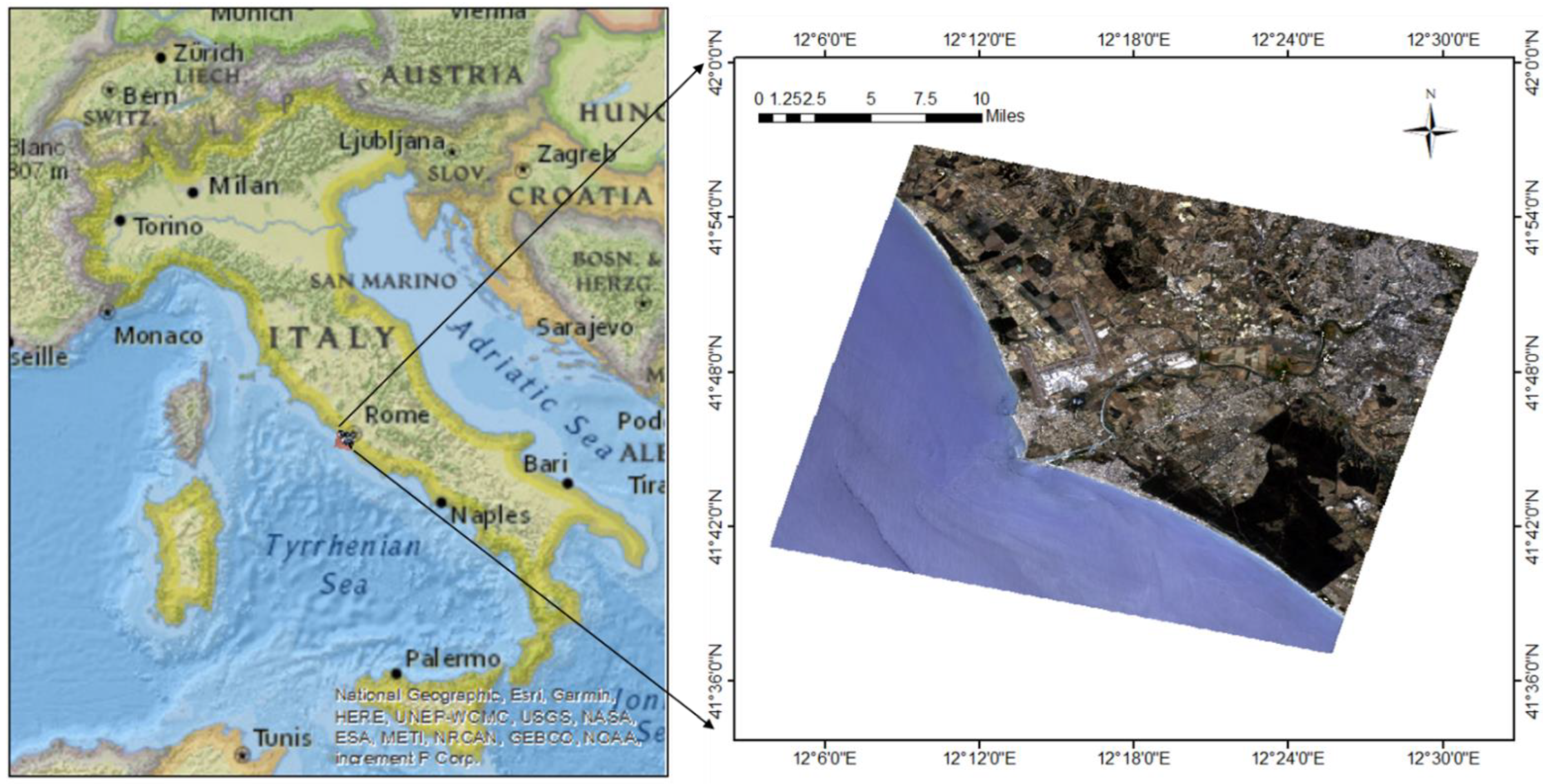
2.1. Study Area
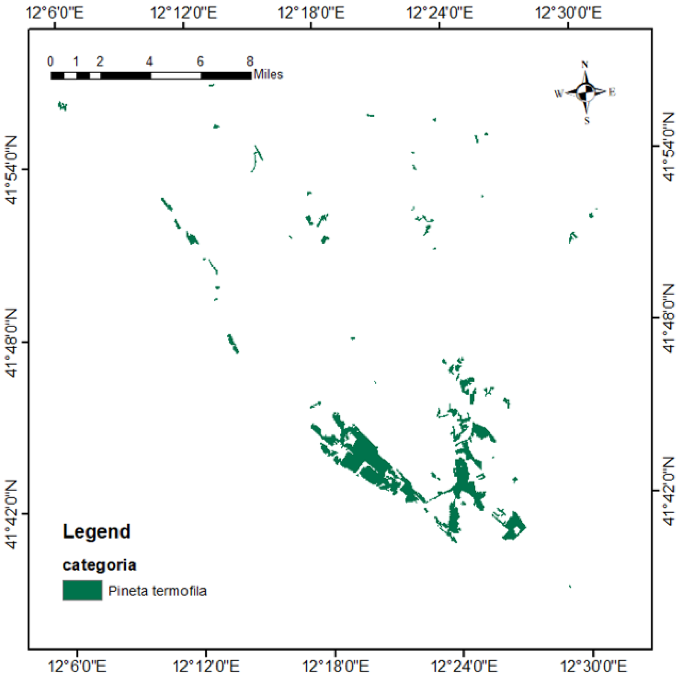
2.2. Reference Data
2.3. Pre-Processing of PRISMA Data
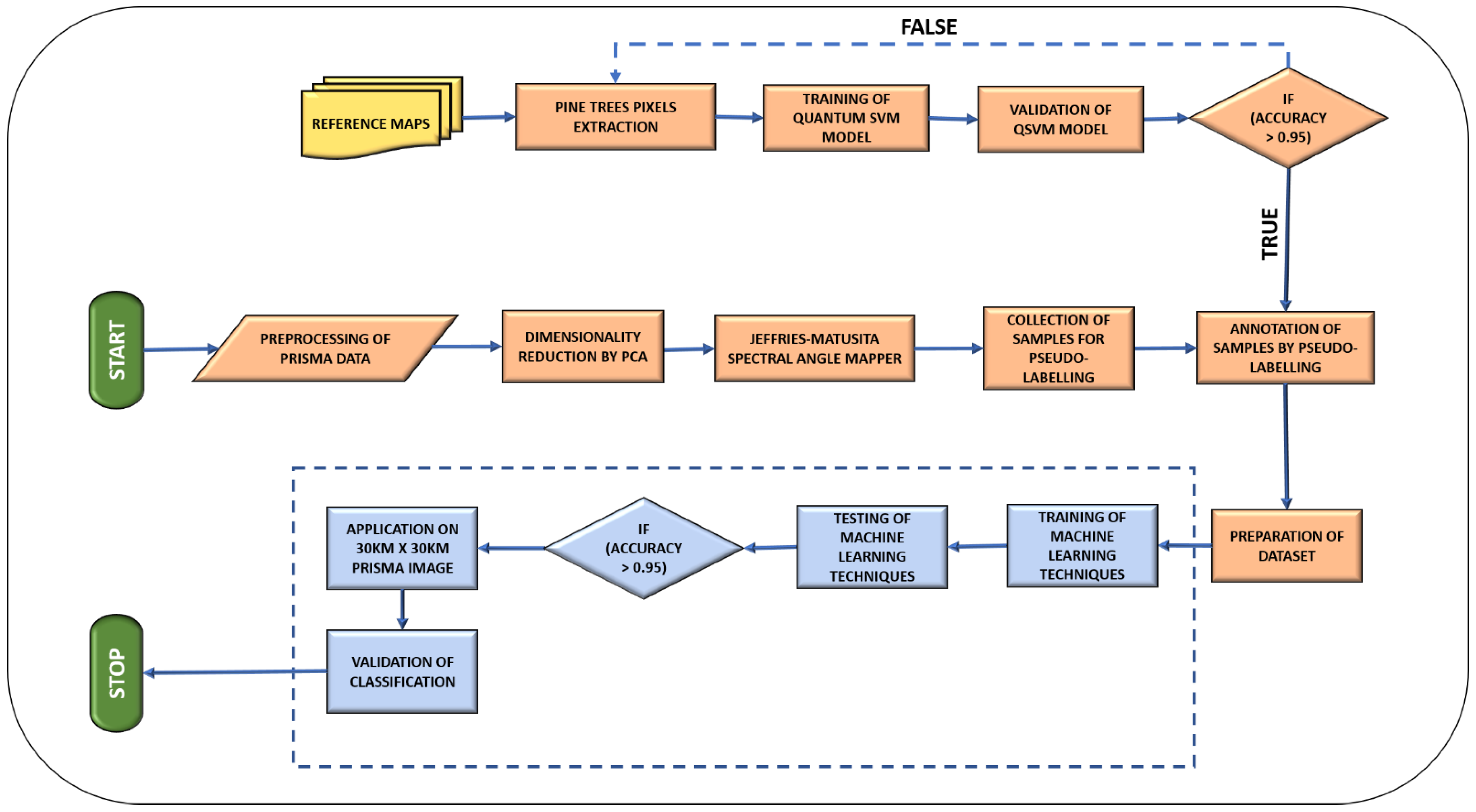
2.4. Implemented Methods
- (1)
- Jeffries Matusita-Spectral Angle Mapper (JM-SAM) is the tangent combination of the most popular SAM technique and Jeffries Matusita distance. SAM provides a spectral angle to detect the intrinsic properties of reflective materials and it has the limitation of insensitivity to illumination and shade effects. So, it is always better to use it in combination with stochastic divergence measures. In this study, the Jeffries Matusita distance involving the exponential factor was used in combination to identify similar spectra [16].
- (2)
- Quantum Support Vector Machine (QSVM) is SVM with a quantum kernel. The significant component that outperforms classical classifiers is the feature map, which has the ability to map d-dimensional non-linear classical data points in quantum state, which plays a key role in pattern recognition. It is difficult to recognise complex patterns of data in original space, especially in learning algorithms, but becomes easy when mapping in higher-dimensional feature space. For more information on the accuracy and processing speeds of QSVM, please refer to [3]. The QISKIT library package was used with Python. QISKIT has three parts: the provider, the backend, and the job. The provider provides access to different backends, such as Aer and IBMQ. Using Aer, the simulator within QISKIT can be availed to run on the local machine, e.g., statevector_simulator, qasm_simulator, unitary_simulator, and clifford_simulator, whereas IBMQ provides access to cloud-based backends [5]. The backend signifies either a real quantum processor or a simulator and can be used to run the quantum circuit and generate results. The execution state, i.e., whether the model is running, queued, or failed, can be found in the third part of QISKIT, the job [5]. One of the backends of IBMQ is “ibmq_qasm_simulator”, which has the features shown in Table 1 [5]. As IBMQ has extensive usage and is a freely available test management solution, it was considered for this study. Maximum accuracy was achieved with 16 qubits [3]. QISKIT packages on Anaconda and the scikit-learn library in Python were used for this classification. The scikit-learn packages of numpy, spectral, matplotlib, time, scipy, math, scipy, pandas, pysptools, os, and gdal were used.
- (3)
- Referring to the literature [1,2,15], some machine learning techniques were selected to find a suitable classifier for the quantum-based pseudo-labelled dataset. The methods implemented in these experiments were support vector machine (SVM), K-nearest neighbour (KNN), random forest (RF), and the boosting methods light gradient boosting machine (LGBM), and extreme gradient boosting (XGBoost). Hybrid ML models were tested by hybridizing a classifier with another classifier and in this study, only hybrid models that provided an accuracy higher than 40% were presented. Hybrid models of SVM-Decision Tree (DCT), RF-SVM, RF-DCT, XGBoost + DCT, XGBoost + RF, and XGBoost + SVM were used. Since we used well-established techniques, a detailed explanation is not provided. Correlations between local spatial features were ignored and deep learning methods were not implemented because we were working with a small dataset.
3. Experimental Procedure
3.1. Quantum-Based Dataset Preparation
3.2. Inputs of ML Classifiers
4. Results
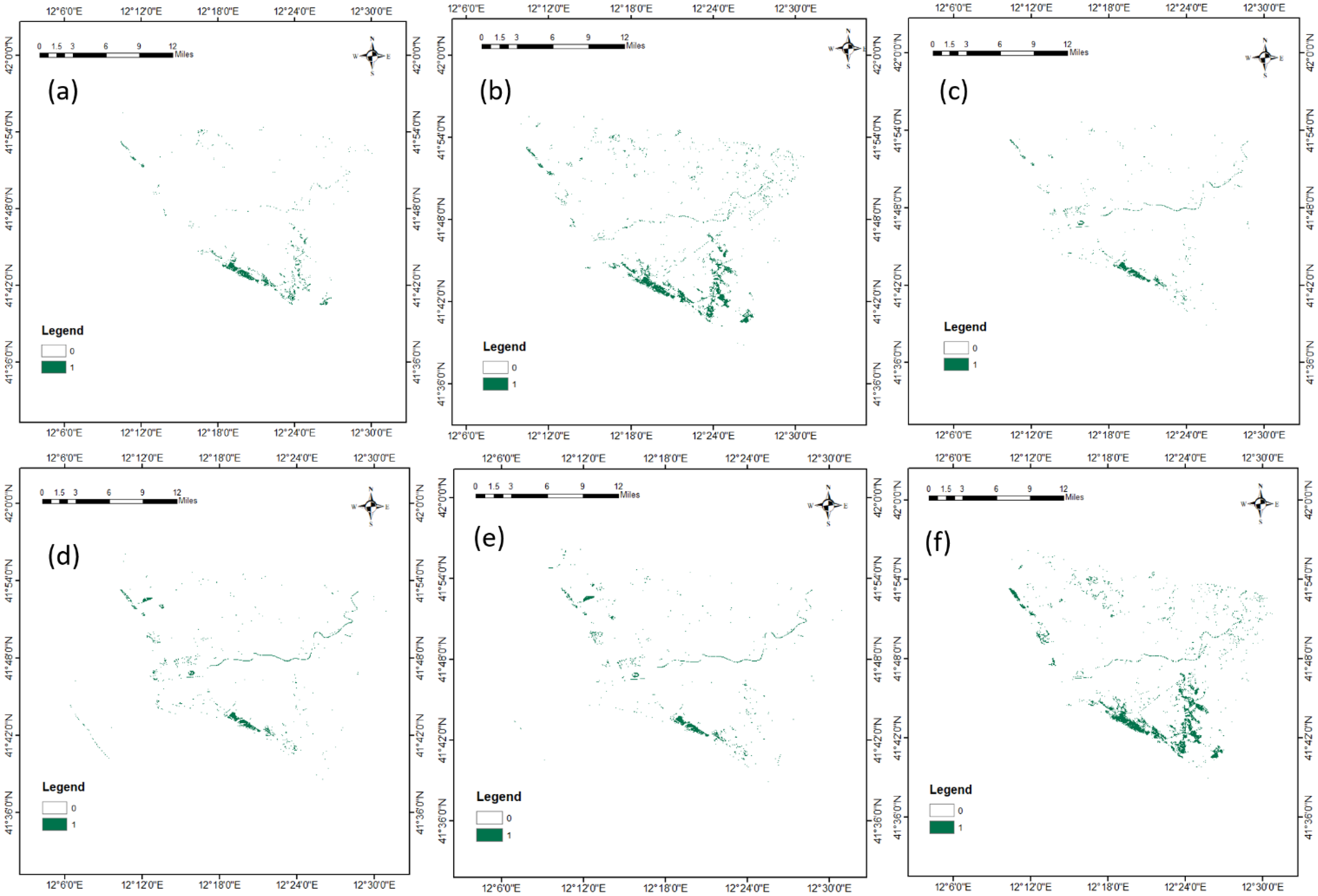
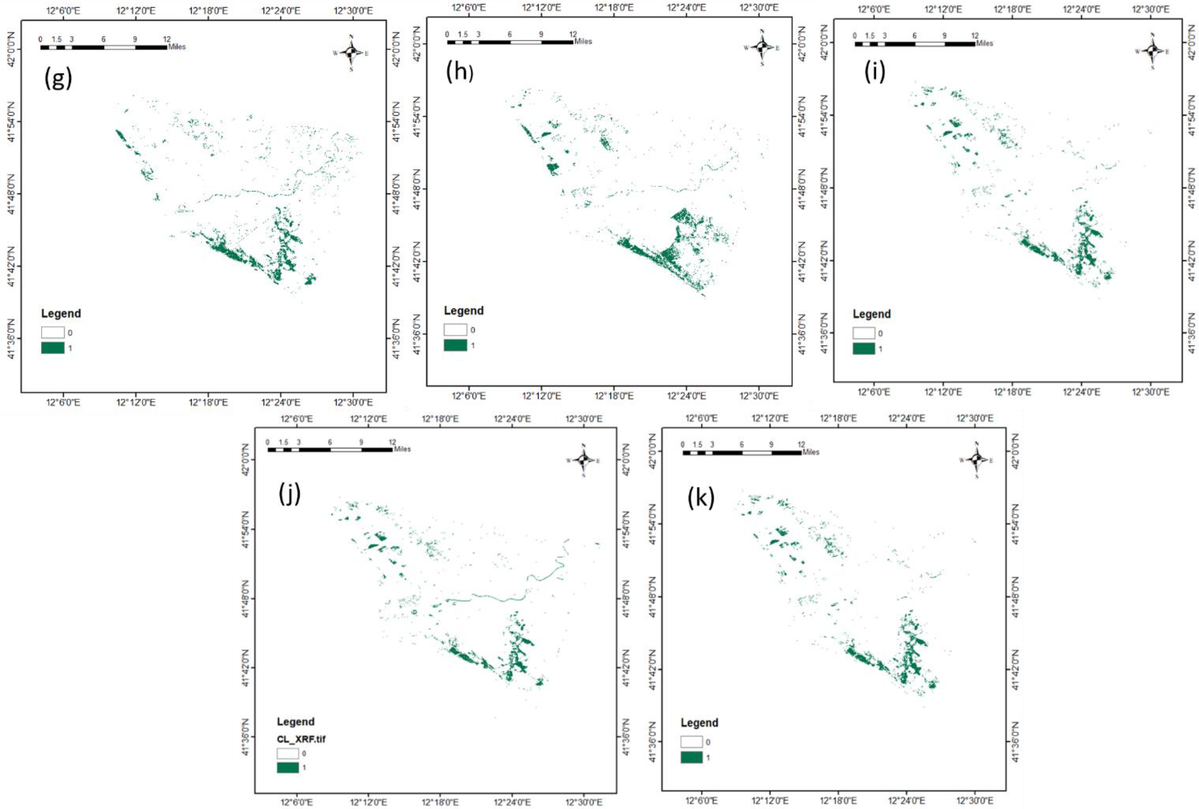
4.1. Classification of Pine Trees
4.2. Validation of the Pine Tree Classification
5. Discussions
6. Conclusions
Author Contributions
Funding
Data Availability Statement
Acknowledgments
Conflicts of Interest
References
- Gewali, U.B.; Monteiro, S.T.; Saber, E. Machine Learning Based Hyperspectral Image Analysis: A Survey. arXiv 2018, arXiv:1802.08701. [Google Scholar]
- Schmitt, M.; Ahmadi, S.A.; Hänsch, R. There is No Data Like More Data—Current Status of Machine Learning Datasets in Remote Sensing. arXiv 2021, arXiv:2105.11726. [Google Scholar]
- Shaik, R.U.; Periasamy, S. Accuracy and processing speed trade-offs in classical and quantum SVM classifier exploiting PRISMA hyperspectral imagery. Int. J. Remote Sens. 2022, 43, 6176–6194. [Google Scholar] [CrossRef]
- Huang, H.Y.; Broughton, M.; Mohseni, M.; Babbush, R.; Boixo, S.; Neven, H.; McClean, J.R. Power of Data in Quantum Machine Learning. Nat. Commun. 2021, 12, 2631. [Google Scholar] [CrossRef] [PubMed]
- Saini, S.; Khosla, P.; Kaur, M.; Singh, G. Quantum Driven Machine Learning. Int. J. Theor. Phys. 2020, 59, 4013–4024. [Google Scholar] [CrossRef]
- Arunachalam, S.; de Wolf, R. Guest Column: A Survey of Quantum Learning Theory 1. ACM SIGACT News 2017, 48, 41–67. [Google Scholar] [CrossRef] [Green Version]
- Biamonte, J.; Wittek, P.; Pancotti, N.; Rebentrost, P.; Wiebe, N.; Lloyd, S. Quantum Machine Learning. Nature 2017, 549, 195–202. [Google Scholar] [CrossRef] [PubMed] [Green Version]
- Ciliberto, C.; Herbster, M.; Ialongo, A.D.; Pontil, M.; Rocchetto, A.; Severini, S.; Wossnig, L. Quantum Machine Learning: A Classical Perspective. Proc. R. Soc. A Math. Phys. Eng. Sci. 2018, 474, 20170551. [Google Scholar] [CrossRef] [PubMed] [Green Version]
- Aaron, B.; Pelofske, E.; Hahn, G.; Djidjev, H.N. Using Machine Learning for Quantum Annealing Accuracy Prediction. Algorithms 2021, 14, 187. [Google Scholar] [CrossRef]
- Cavallaro, G.; Dennis, W.; Madita, W.; Kristel, M.; Morris, R. Approaching Remote Sensing Image Classification with Ensembles of Support Vector Machines on the D-Wave Quantum Annealer. In Proceedings of the IGARSS 2020—2020 IEEE International Geoscience and Remote Sensing Symposium, Waikoloa, HI, USA, 26 September–2 October 2020; pp. 1973–1976. [Google Scholar] [CrossRef]
- Otgonbaatar, S.; Datcu, M. A Quantum Annealer for Subset Feature Selection and the Classification of Hyperspectral Images. IEEE J. Sel. Top. Appl. Earth Obs. Remote Sens. 2021, 14, 7057–7065. [Google Scholar] [CrossRef]
- Liu, Y.; Arunachalam, S.; Temme, K. A Rigorous and Robust Quantum Speed-Up in Supervised Machine Learning. Nat. Phys. 2021, 17, 1013–1017. [Google Scholar] [CrossRef]
- Pepe, M.; Pompilio, L.; Gioli, B.; Busetto, L.; Boschetti, M. Detection and Classification of Non-Photosynthetic Vegetation from Prisma Hyperspectral Data in Croplands. Remote Sens. 2020, 12, 3903. [Google Scholar] [CrossRef]
- Shaik, R.U.; Giovanni, L.; Fusilli, L. New Approach of Sample Generation and Classification for Wildfire Fuel Mapping on Hyperspectral (Prisma) Image. In Proceedings of the 2021 IEEE International Geoscience and Remote Sensing Symposium IGARSS, Brussels, Belgium, 11–16 July 2021. [Google Scholar] [CrossRef]
- Amato, U.; Antoniadis, A.; Carfora, M.F.; Colandrea, P.; Cuomo, V.; Franzese, M.; Pignatti, S.; Serio, C. Statistical Classification for Assessing Prisma Hyperspectral Potential for Agricultural Land Use. IEEE J. Sel. Top. Appl. Earth Obs. Remote Sens. 2013, 6, 615–625. [Google Scholar] [CrossRef]
- Shaik, R.U.; Laneve, G.; Fusilli, L. An Automatic Procedure for Forest Fire Fuel Mapping Using Hyperspectral (PRISMA) Imagery: A Semi-Supervised Classification Approach. Remote Sens. 2022, 14, 1264. [Google Scholar] [CrossRef]
- Huang, Z.; Wu, W.; Liu, H.; Zhang, W.; Hu, J. Identifying Dynamic Changes in Water Surface Using Sentinel-1 Data Based on Genetic Algorithm and Machine Learning Techniques. Remote Sens. 2021, 13, 3745. [Google Scholar] [CrossRef]


| Properties | ibmq_qasm_simulator |
|---|---|
| Provider | Ibmq-q/open/main |
| status_msg | Active |
| n_qubits | 32 |
| backend_version | 0.1.547 |
| basic_gates | U1, U2, U3, U, DELAY, P, R, RX, RY, RZ, ID, X, Y, Z, H, S, SDG, SX, T, TDG, MULTIPLEXER, INITIALIZE, KRAUS, ROERROR, SWAP, CX, CY, CZ, CSX, CP, CU1, CU2, CU3, RXX, RYY, RZZ, RZX, CCX, CSWAP, MCX, MCY, MCZ, MCSX, MCP, MCU1, MCU2, MCU3, MCRX, MCRY, MCRZ, MCR, MCSWAP, UNITARY, DIAGONAL |
| max_circuits | 300 |
| max_shots | 100,000 |
| max_qubits per pulse gate | 3 |
| max_channels per pulse gate | 9 |
| S.No | Machine Learning Technique | Hyperparameters Range |
|---|---|---|
| 1 | SVM | C = (1,10,100), kernel = rbf and Gamma = (1 × 10⁻³ to 10) |
| 2 | KNN | n_neighbors = (5,7,9,11,13,15), weights = (‘uniform’, ’distance’), metric = (‘minkowski’, ’euclidean’, ’manhattan’) |
| 3 | Random Forest | Bootstrap = (True, False), max_depth = (5,10,15,30), max_features = (2,3,5), min_sample_leaf = (2,5,10,100), min_sample_split = (2, 5, 10, 100), n_estimators = (100, 500) |
| 4 | LGBM | Learning_rate = (0.005, 0.01,0.01), n_estimator = (500), num_leaves = (6,30,50), boosting_type = (dart), max_depth = (1,3,5), max_bin = (225), reg_alpha = (1,1.2), reg_lambda = (1,1.2,1.4) |
| 5 | XGBoost | min_child_weight = (1,3,5), subsample = (0.5,0.7) |
| 6 | Decision Tree | max_depth = (1,6,8,11), min_sample_split = (1,9,11), min_sample_leaf = (1,3,7,9) |
| S.No | Machine Learning Technique | Validation Result | Time Taken (in Hours) | View on Classification Result |
|---|---|---|---|---|
| 1 | SVM | Classified Points = 243/300 Accuracy ≅ 80% | >2 | This model classified the pine trees and presented lower misclassification (less than 20%) of other vegetation. |
| 2 | KNN | Classified Points = 239/300 Accuracy ≅ 80% | >1 | This model classified the pine trees and presented higher misclassification (higher than 20%) of other vegetation (especially on upper part of the image). |
| 3 | Random Forest | Classified Points = 182/300 Accuracy ≅ 60% | >7 | Random forest did not classify all the pine trees; however, there were no misclassifications. |
| 4 | LGBM | Classified Points = 177/300 Accuracy ≅ 60% | >4 | LGBM did not classify all the pine trees; however, there were no noticeable misclassifications. |
| 5 | XGBoost | Classified Points = 182/300 Accuracy ≅ 60% | >1 | There was only a slight variation in XGBoost in comparison with LGBM, i.e., XGBoost classified a few more spots; however, the classification was insufficient. |
| 6 | SVC + Decision Tree | Classified Points = 241/300 Accuracy ≅ 80% | <1 | This model classified the pine trees very well, especially in the bottom part of the image. |
| 7 | Random Forest + SVC | Classified Points = 122/300 Accuracy ≅ 40% | <1 | This model misclassified other vegetation. |
| 8 | Random Forest + Decision Tree | Classified Points = 120/300 Accuracy ≅ 40% | <1 | This model misclassified other vegetation. |
| 9 | XGBoost + Decision Tree | Classified Points = 262/300 Accuracy ≅ 86% | <1 | This hybrid model classified the pine trees very well in the bottom region; however, it misclassified the top part. |
| 10 | XGBoost + Random Forest | Classified Points = 254/300 Accuracy ≅ 83% | <1 | This hybrid model classified the pine trees very well in the bottom region; however, it misclassified the top part. |
| 11 | XGBoost + SVC | Classified Points = 255/300 Accuracy ≅ 83% | <1 | This hybrid model classified the pine trees very well in the bottom region; however, it misclassified the top part. |
Publisher’s Note: MDPI stays neutral with regard to jurisdictional claims in published maps and institutional affiliations. |
© 2022 by the authors. Licensee MDPI, Basel, Switzerland. This article is an open access article distributed under the terms and conditions of the Creative Commons Attribution (CC BY) license (https://creativecommons.org/licenses/by/4.0/).
Share and Cite
Shaik, R.U.; Unni, A.; Zeng, W. Quantum Based Pseudo-Labelling for Hyperspectral Imagery: A Simple and Efficient Semi-Supervised Learning Method for Machine Learning Classifiers. Remote Sens. 2022, 14, 5774. https://doi.org/10.3390/rs14225774
Shaik RU, Unni A, Zeng W. Quantum Based Pseudo-Labelling for Hyperspectral Imagery: A Simple and Efficient Semi-Supervised Learning Method for Machine Learning Classifiers. Remote Sensing. 2022; 14(22):5774. https://doi.org/10.3390/rs14225774
Chicago/Turabian StyleShaik, Riyaaz Uddien, Aiswarya Unni, and Weiping Zeng. 2022. "Quantum Based Pseudo-Labelling for Hyperspectral Imagery: A Simple and Efficient Semi-Supervised Learning Method for Machine Learning Classifiers" Remote Sensing 14, no. 22: 5774. https://doi.org/10.3390/rs14225774