
Tree Species Classification Using Ground-Based LiDAR Data by Various Point Cloud Deep Learning Methods
by
 , , ,
, , ,
Bingjie Liu
1 ,
,
Huaguo Huang
1 ,
,
Yong Su
2 ,
,
Shuxin Chen
3,
Zengyuan Li
3,
Erxue Chen
3 and
Xin Tian
3,* 1
Research Center of Forest Management Engineering of State Forestry and Grassland Administration, Beijing Forestry University, Beijing 100083, China
2
College of Forestry, Southwest Forestry University, Kunming 650224, China
3
Institute of Forest Resource Information Techniques, Chinese Academy of Forestry, Beijing 100091, China
*
Author to whom correspondence should be addressed.
Remote Sens. 2022, 14(22), 5733; https://doi.org/10.3390/rs14225733
Submission received: 17 August 2022
/
Revised: 5 November 2022
/
Accepted: 10 November 2022
/
Published: 13 November 2022
(This article belongs to the Collection Feature Paper Special Issue on Forest Remote Sensing)
Abstract
:Tree species information is an important factor in forest resource surveys, and light detection and ranging (LiDAR), as a new technical tool for forest resource surveys, can quickly obtain the 3D structural information of trees. In particular, the rapid and accurate classification and identification of tree species information from individual tree point clouds using deep learning methods is a new development direction for LiDAR technology in forest applications. In this study, mobile laser scanning (MLS) data collected in the field are first pre-processed to extract individual tree point clouds. Two downsampling methods, non-uniform grid and farthest point sampling, are combined to process the point cloud data, and the obtained sample data are more conducive to the deep learning model for extracting classification features. Finally, four different types of point cloud deep learning models, including pointwise multi-layer perceptron (MLP) (PointNet, PointNet++, PointMLP), convolution-based (PointConv), graph-based (DGCNN), and attention-based (PCT) models, are used to classify and identify the individual tree point clouds of eight tree species. The results show that the classification accuracy of all models (except for PointNet) exceeded 0.90, where the PointConv model achieved the highest classification accuracy for tree species classification. The streamlined PointMLP model can still achieve high classification accuracy, while the PCT model did not achieve good accuracy in the tree species classification experiment, likely due to the small sample size. We compare the training process and final classification accuracy of the different types of point cloud deep learning models in tree species classification experiments, further demonstrating the advantages of deep learning techniques in tree species recognition and providing experimental reference for related research and technological development.
1. Introduction
Forest ecosystems cover approximately one-third of the Earth’s land surface and are an important type of global land cover [1]. Forests have an irreplaceable role in maintaining the stability of ecosystems and play a vital role in the survival and development of human civilization [2,3]. Tree species information is essential in forest resource surveys, and the classification of tree species is one of the main tasks of forest science [4]. Timely and accurate information on tree species is essential for developing strategies for the sustainable management and conservation of planted and natural forests [5]. Over the past four decades, the development of remote sensing technology has made large-scale forest inventories possible. Light detection and ranging (LiDAR), as an active remote sensing technology, can obtain 3D point clouds of scanned forest scenes and has become the main technical tool for tree species identification and accurate extraction of forest parameters.
LiDAR data from different platforms have different roles in the study of forest parameter extraction and tree species classification. Most studies have used airborne laser scanning (ALS) data, from which scholars extract taxonomic features for region-wide mapping of tree species distribution [6,7,8,9]; however, there are relatively few studies using terrestrial laser scanning (TLS) data for individual tree species classification due to its high acquisition cost and difficulty in data processing [10,11]. Mobile laser scanning (MLS) based on simultaneous localization and mapping (SLAM) technology can easily and quickly collect point cloud data in a study area [12]. Research on the identification and classification of individual tree point cloud species based on ground-based LiDAR data extraction has been carried out by various scholars [13,14,15].
Based on traditional machine learning algorithms, LiDAR-derived feature metrics help to improve the accuracy of tree species identification [16]. Random forests (RF) [17,18,19,20] and support vector machines (SVM) [21,22,23] have been used in many studies. However, machine learning-based classification methods require the prior extraction of a large number of classification features, and the accuracy of these algorithms depends on a variety of feature metrics. Deep learning approaches, as end-to-end classifiers, can automatically extract classification features through the use of deep neural networks. Existing research has demonstrated that high classification accuracy can be achieved through the use of deep learning for tree species classification [8,9,14].
Over the past decade, deep learning has made rapid progress in the field of computer vision. Point clouds are disordered and do not conform to the regular lattice grid in 2D images, making it difficult to apply traditional convolutional neural networks (CNNs) to such unordered inputs. Therefore, scholars have developed a series of deep learning models based on the characteristics of 3D point cloud data, in addition to a series of deep learning models applicable to point clouds. The development of point cloud analysis has been closely related to the development of image processing networks [24]. PointNet [25] and PointNet++ [26], as seminal studies in point-based deep learning, have driven the development of deep learning modeling techniques that learn categorical feature information directly from the original point cloud. In current research, point cloud deep learning methods can be classified into pointwise multi-layer perceptron (MLP), convolution-based, graph-based, and attention-based methods, depending on the point-based feature-learning network architecture [27,28]. Most existing deep learning methods used in studies for individual tree point cloud tree species classification are based on pointwise MLP. Other types of point cloud deep learning methods have rarely been used in tree species classification studies. In response to the limitations of point cloud deep learning models regarding the number of points in typical samples, the non-uniform grid-based downsampling algorithm, used in the studies [14,29], has shown potential for accurately extracting the 3D morphology of single plants. Zhou et al. [30] proposed CNN-specific [31] class activation maps (CAMs) for the visualization of class features, which represent a weighted linear sum of each class of visual patterns present at different spatial locations in the image [30]. In this line, Huang et al. [32] have attempted to interpret the PointNet model through the use of CAMs, and Xi et al. [11] have visualized the feature points of PointNet++ classification results using CAMs.
To fully explore the potential of point cloud deep learning methods with regard to the classification of individual tree species, we conducted the following experiments. A point cloud data downsampling strategy (NGFPS) that incorporates non-uniform grid and farthest point sampling methods was proposed. Four different types of point cloud deep learning approaches, including pointwise MLP, convolution-based, graph-based, and attention-based models, were used for tree species classification and recognition of individual tree point clouds. A total of six point cloud deep learning models—including PointNet [25], PointNet++ [26], PointMLP [24], PointConv [33], DGCNN [34], and point cloud transformer (PCT) [35]—were included in our experiments. We analyzed and evaluated the classification results of all models. The CAM method was used to visualize the set of critical points at which the classification features of a sample converge. Some new results regarding tree species classification using point cloud deep learning methods were presented, thus providing a reference for future tree species classification and the further development of deep learning models.
2. Materials and Methods
2.1. Study Area and Data Collection
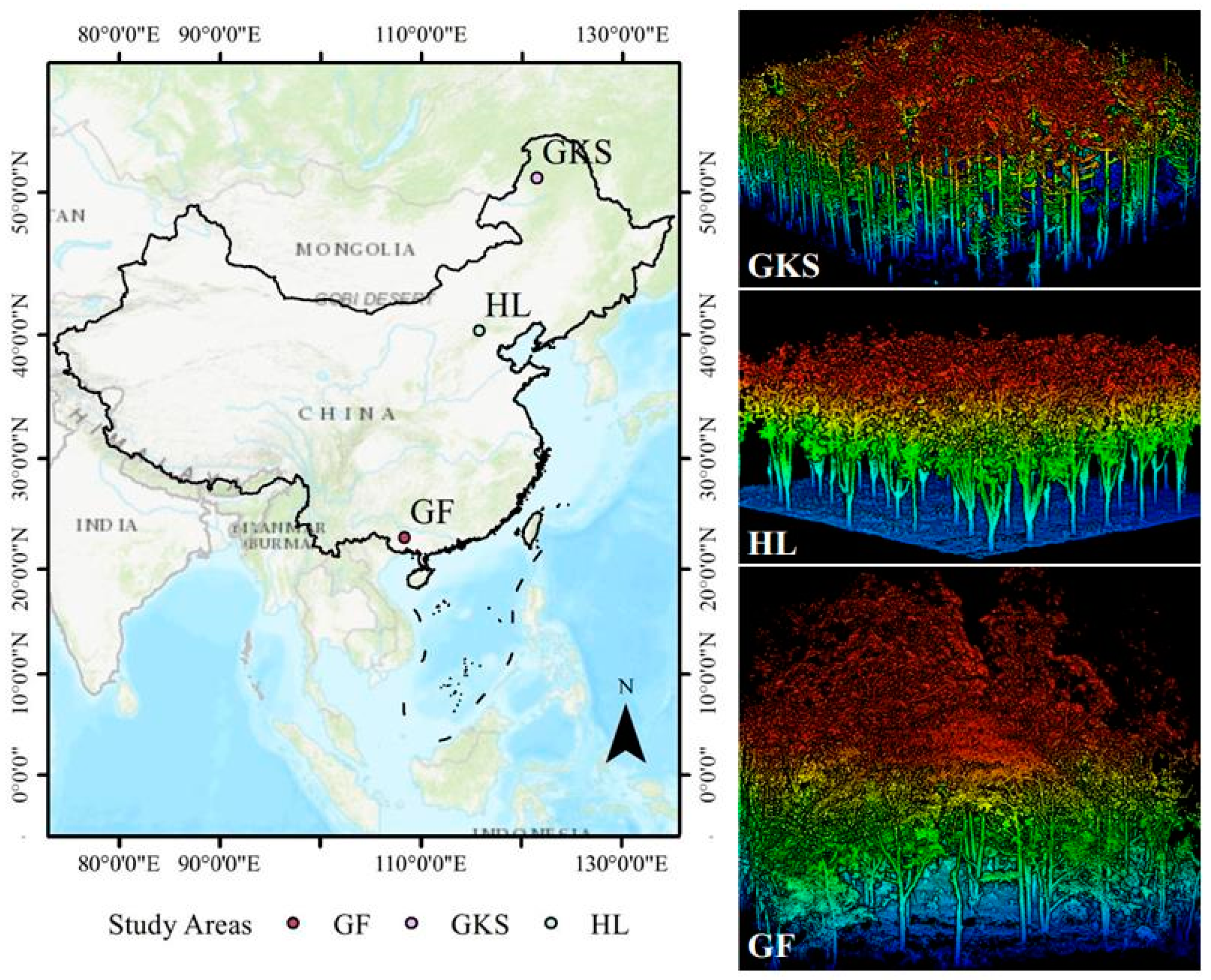
Experimental data were collected from three study areas in China: The Greater Khingan Station (GKS), Huailai Remote Sensing Comprehensive Experimental Station (HL), and Gaofeng forest farm (GF). Point cloud data from forest plots in the study areas were collected in September, July, and April of 2021, using a LiBackpack DGC50 backpack laser scanning (BLS) system from Beijing GreenValley Technology Co., Ltd. (Beijing, China). The LiBackpack DGC50 system has an absolute accuracy of ±5 cm, a relative accuracy of 3 cm, and is equipped with two VLP 16 laser sensors that can reach a scanning range of 100 m, with vertical and horizontal scanning angles of −90° to 90° and 360°, respectively. Figure 1 shows the distribution locations of the three study areas and the LiDAR data of some sample sites. LiDAR data were collected from 17, 41, and 16 ground sample plots in the three experimental areas of GKS, HL, and GF, respectively. A total of eight types of tree species were included in the three experimental areas. Table 1 provides a detailed representation of tree species and forest plot information.
2.2. Data Pre-Processing
The data collected in the field were SLAM solved using the LiFuser-BP software, in order to obtain the raw point cloud data in standard format. To obtain individual tree point cloud data that fit the input requirements of the deep learning model, the LiDAR data of the plots collected in the field were subjected to a series of pre-processing steps.
First, the noise in the point cloud data was removed. A height threshold method was used to remove noise points that were significantly above and below ground level, and a local distribution-based algorithm was used to remove some stray isolated points. Then, we used the cloth simulation filtering (CSF) algorithm [36] to classify the raw point cloud data into two categories: ground points and vegetation points. To segment the point cloud of each tree from the point cloud of the whole plot, we normalized the point cloud of the plot based on the elevation information of the ground points, which were processed to be parallel to the horizontal plane. Subsequently, we eliminated the ground points and segmented the point cloud of each individual tree from the sample point cloud using the comparative shortest path (CSP) algorithm [37], which uses a bottom-up approach to detect each tree in the region. Immediately afterwards, we processed the point cloud data of each single tree manually and eliminated some points that were misclassified, such as ground and weeds. Finally, we obtained clean point cloud data for each tree.
An individual tree point cloud data set for tree species classification, called TS8, was successfully built following the file organization of the ModelNet40 [38] dataset, which has been commonly used in point cloud deep learning research. As we obtained an unbalanced number of trees of each species, we used a stratified random sampling method within species, randomly selecting 80% of each tree species as the training data set and the remaining 20% as the test set.
2.3. Research Workflow
After creation of the TS8 (Table 1) data set, we downsampled the individual tree point clouds using the proposed NGFPS method. The data set was then trained for classification using a variety of deep learning models. Finally, high-precision tree species classification results and optimal model hyperparameters were obtained. Figure 2 depicts the technical route and logical structure of this study in detail.
3. Methods
3.1. Methods Combined with Non-Uniform Grid and Farthest Point Sampling
The difference between the non-uniform grid sampling (NGS) method and traditional grid-/voxel-based methods is that it can select representative points from a grid having different sizes. The NGS method calculates the normal vector of each point before sampling the point cloud, which can better preserve the details of 3D objects. The NGS method was first used to align multiple sets of point clouds representing the same object but with different coordinate systems [39], as well as for 3D point cloud surface reconstruction [40,41,42]. This method can effectively filter out the key points describing the shape of the object from a dense point cloud and is more conducive to the mutual matching of multiple groups of point clouds, as it can well-preserve the details of the 3D object‘s surface. The dominant downsampling method used with current deep learning models is the farthest point sampling (FPS) method, which allows for rapid sampling to obtain a point cloud of objects containing a specified number of points (N = 1024, 2048, …). One of the main reasons for using the FPS method is that the ModelNet40 data set consists of point clouds uniformly sampled from the surface of regular computer-aided design (CAD) models; however, in practice, the point cloud density of collected LiDAR data is not uniformly distributed, and the points that can represent the details of the object need to be fully retained when identifying and classifying tree species.
FPS is a downsampling method for uniform density point clouds, which cannot successfully retain the more detailed features of tree point clouds. In the study of tree species classification, more detailed information regarding 3D objects needs to be retained using NGS methods. However, the NGS method cannot accurately obtain the number of points (N) contained in the sample required by the point cloud deep learning model. Therefore, in this experiment, we first used the NGS method to obtain the number of points in the individual tree point cloud that is closest to N. After obtaining samples with sufficient detail retention, the number of points in the individual tree point cloud can be unified using the FPS method.
The NGS algorithm can be implemented quickly in MATLAB, but requires inputting the smallest number of points (k) within each grid point as the initial parameter, and the final sampling results in the representation of k points combined into 1 point. To obtain a fixed number of downsampling points N per object, the value of k tends to be inconsistent during data processing. In order to obtain individual tree point cloud data that are more conducive to model learning, we combine two methods, non-uniform grid and farthest point sampling, and the combined method is called NGFPS in this paper. The details of the combination of the two methods are as follows.
- The objects are downsampled using the NGS algorithm, and k is iterate as an input parameter. The minimum value of k is set to 6, and the value of k is increased by 1 at each iteration;
- When the number of points satisfies N(k) < N after downsampling the object, the iteration is stopped, and the experimental results of N(k−1) are retained;
- We use the FPS algorithm to downsample the N(k−1) points to the specified number of points N.
Using the NGFPS method not only preserves the details of the 3D objects better, but also allows us to obtain a data set that satisfies the number of points N as the input to the deep learning model.
3.2. Point Cloud Deep Learning Methods
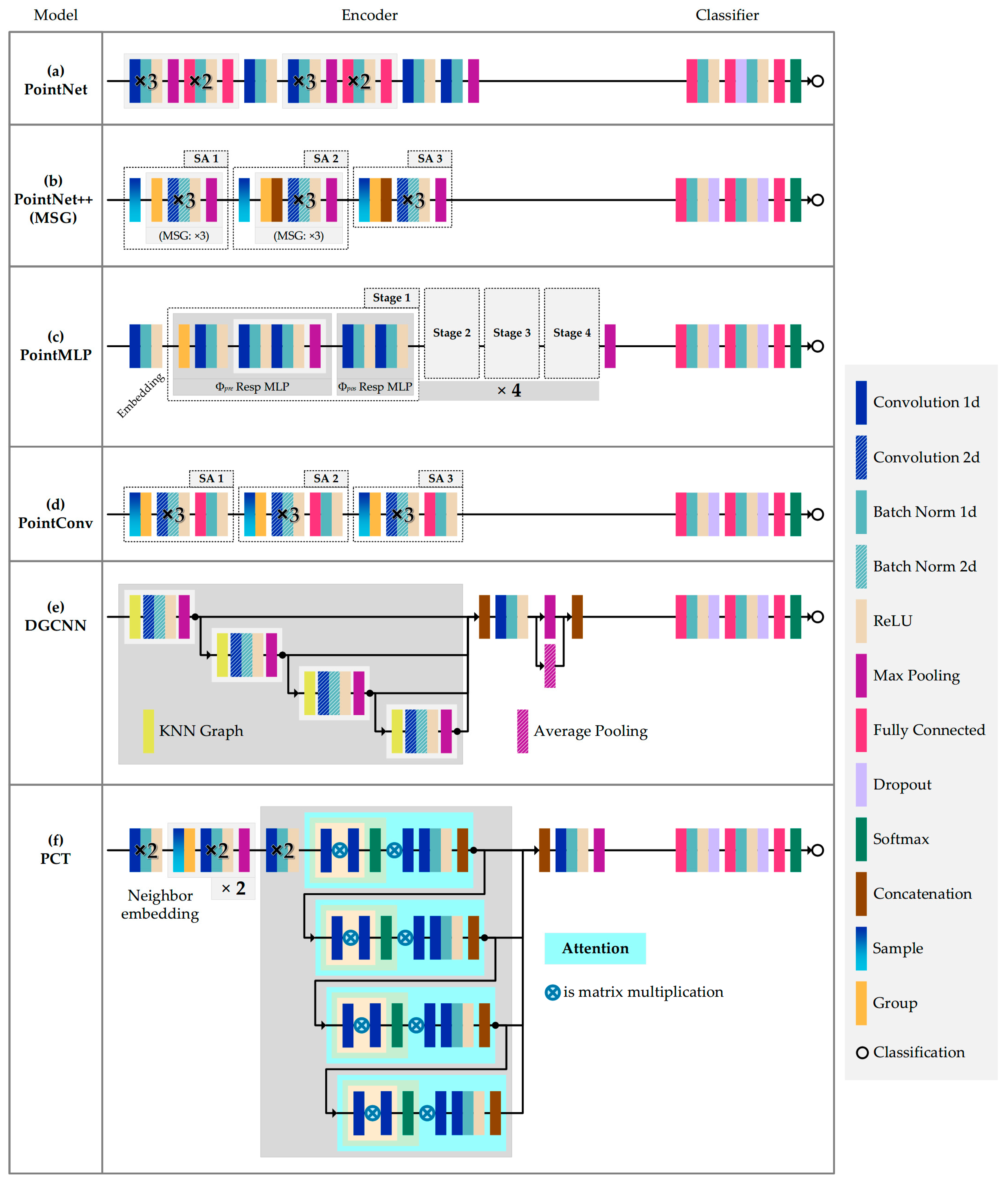
We conducted tree species classification research using four types of point cloud deep learning approaches: pointwise MLP, convolution-based, graph-based, and attention-based models. The second module in Figure 2 shows the categories of models used, along with the names of the specific models. To facilitate comparison and analysis of the models, the structures of all models are summarized and drawn in a single image (Figure 3). Additionally, the hyperparameters used in the training process of all the deep learning models are summarized in Table 2. We maintained the parameters used by the original authors of the models as much as possible.
3.2.1. Pointwise MLP Methods
Multi-layer perceptrons (MLPs), developed from perceptrons, are the simplest kind of deep network. An MLP is a non-linear model obtained by adding hidden layers and activation functions, as well as changing the classification function. Commonly used activation functions include sigmoid, tanh, ReLU, and so on. The softmax function is used to address multi-classification problems. The number of hidden layers and the size of each layer are its main hyperparameters.
Due to the irregularity of point cloud data, traditional 2D deep learning methods cannot be directly used with 3D data. PointNet is a pioneering work that deals directly with disordered point sets using multiple shared MLPs, which achieves permutation invariance through symmetric functions. PointNet uses multiple MLP layers to learn point-wise features independently, as well as a maximum pooling layer to extract global features (see Figure 3a). This model has three main modules: A symmetric function aggregating information from all points, a combination of local and global information, and a joint alignment network. The global features extracted by the model are classified using a multi-layer perceptron classifier. The PointNet model can be expressed by Equation (1):
where is the set of points of the model input, and are multi-layer perceptron networks, and the function is invariant to the arrangement of the points of the model input.
As the features of each point in PointNet are learned independently, the local structure generated by the metric space points cannot be captured, which limits its ability to recognize fine-grained patterns and generalize to complex scenes. PointNet++ introduces a hierarchical feature learning paradigm that captures the fine geometric structure from the neighborhood of each point. Due to its ability to obtain local feature information at different scales of 3D objects, PointNet++ has become the basis for the development and exploitation of many other models [34,43,44]. As the core of the PointNet++ hierarchy, its set abstraction layer (SA) consists of three layers: A sampling layer, a grouping layer, and a PointNet-based learning layer. The SA in Figure 3b represents the structure of the model. The input of each SA module can be represented by a matrix of size N × (d + C), where N denotes the number of points of the 3D object, d denotes the coordinate dimension, and C denotes the feature dimension. The structure after SA processing is N’ × (d + C’).
(1) The points in each layer of the input are first downsampled using the FPS method. Compared with random sampling, FPS provides better coverage of the entire point set for the same number of points [26].
(2) The sampled data are subsequently grouped using a ball query method, which allows for better generalization of local area features in space. The output is N’ × K × (d + C), where K denotes the number of points contained in each query ball.
(3) Finally, the PointNet layer is used to learn the features of the grouped data.
PointNet++ learns features from local geometric structures by stacking multiple levels of ensemble abstraction and abstracting local features in a layer-wise manner. The core structure of the model can be expressed as Equation (2):
where denotes the maximum pooling operation, denotes the MLP local feature extraction function, and denotes the feature of the jth neighboring point of the ith sampling point. In this experiment, the distribution of the point cloud density of our collected LiDAR data is heterogeneous, so a multi-scale grouping (MSG) approach was used. A simple but effective way of capturing multi-scale features is to use MSG. Features of different scales are connected in series to form multi-scale features.
PointMLP is a deep residual MLP network that follows the design philosophy of PointNet and PointNet++, using a simpler but deeper network architecture explored by Ma et al. [24]. PointMLP uses pre-feedback residual MLP network to hierarchically aggregate the local features extracted by MLP without any fine-grained local feature extractor. Thus, this method can avoid the large computational effort and continuous memory access caused by complex local feature extraction. A lightweight geometric affine module is also introduced, in order to adaptively convert local points to a normal distribution, further improving the performance and generalization capability of the model. The structure of the model is shown in Figure 3c, and the core algorithm of this network can be expressed as Equation (3):
where and are residual MLP modules, the shared is used to learn shared weights from local regions, and is used to extract deep aggregated features. The aggregation function is the maximum pooling function. The model uses the k-nearest neighbor algorithm (k-NN) to select proximity points with a value of k = 24. Equation (3) describes a phase of PointMLP. We use a four-layer deep network, so it is necessary to repeat this computational procedure four times.
Ma et al. [24] have also proposed a lightweight version, PointMLP-elite, which reduces the number of channels in the PointMLP intermediate FC layer by a factor of 4, slightly adjusts the network architecture, and reduces the number of MLP blocks and embedding dimensions.
3.2.2. Convolution-Based Method
PointConv [33] is one of the best convolution-based methods. PointConv is an extension of the Monte Carlo approximation of the 3D continuous convolution operator. By using the continuous weights and density functions in the MLP approximation convolution filter, PointConv is able to extend the dynamic filter to new convolution operations. The point cloud is represented as a set of 3D points , where each point is a vector containing location features. PointConv is a substitution-invariant point cloud operation that can make point clouds compatible with convolution. PointConv can be expressed as follows:
where represents the inverse density of , and represents the characteristics of the points centered at point in local region . For each local region, can be any position within the region.
PointConv approximates the weight function from the 3D coordinates by a multi-layer perceptron and approximates the inverse density through kernelized density estimation and a non-linear transformation implemented with an MLP. The weights of the MLP are shared over all points, in order to maintain permutation invariance. The density of each point in the point cloud is estimated using kernel density estimation, following which the density is input to the MLP for one-dimensional non-linear transformation, resulting in the inverse density scale .
Considering the high memory consumption and low efficiency of the PointConv implementation, Wu et al. [33] have simplified the model to two standard operations: matrix multiplication and 2D convolution.
3.2.3. Graph-Based Method
Point clouds have difficulties, in terms of processing directly using convolution, due to their disorderly and irregular characteristics. Graph-based approaches use graphs to study the relationships between points. Wang et al. [34] have designed the DGCNN model and proposed a new neural network module, called EdgeConv, to generate edge features describing the relationship between points and their neighbors. It constructs a local graph, which preserves the relationships between points. EdgeConv dynamically constructs a graph structure at each layer of the network, using each point as a centroid to characterize the edge feature with each neighboring point, and then aggregates these features to obtain a new representation of that point. EdgeConv is one of the main components of the DGCNN structure. The set of points is defined as , where each point is a vector containing the features at a location . The directed graph of the local point cloud structure can be represented as:
where denotes the vertices and denotes the edges. In the simplest case, is defined as the k-nearest neighbors (k-NN) graph of the point set . The edge features are defined as:
where is a set of non-linear functions with learnable parameters . The edge features are defined using the channel symmetric aggregation function associated with all the edges from each vertex. The output of EdgeConv at the ith vertex can be expressed as:
where . Equation (8) can preserve the global features in the neighborhood, as well as the information of the local neighborhood. The edge features are obtained by adding the perceptron in Equation (9), while the aggregation operation is implemented using Equation (10).
Another major part of the DGCNN structure is the dynamic update graph. The graph is recomputed using the nearest neighbors in the feature space generated at each layer. Therefore, at each layer l, there is a different graph . The DGCNN learns how to construct the graph used in each layer, which is its largest difference from the GCN.
3.2.4. Attention-Based Method
Attention-based methods have also shown excellent capabilities for relationship exploration, such as PCT [35] and Point Transformer [45,46]. The attention module is the core component, which generates refined attention features for input features, based on the global context. Attention allows the model to adapt to diverse data by calculating dynamic weights. The self-attention (SA) module is the core component, generating refined attention features as its input features based on the global context. Self-attention is a mechanism that calculates the semantic affinities between different items within a sequence of data. Self-attention updates the features at each location by computing a weighted sum of features using pairs of affinities at all locations to capture the long-range dependencies in a single sample.
The transformer does not care about the order of the input data. For point cloud data, the transformer itself is permutation-invariant, and feature learning is performed through an attention mechanism. As such, they are considered very suitable for implementing point cloud deep learning models. The overall structure and details of the PCT model are shown in Figure 3f. The PCT model encoder is made up of an input embedding module and four stacked attention modules. The encoder initially embeds the input 3D point coordinates into a new feature space. The embedded features are then passed into the four stacked attention modules, which are used to learn each point‘s features. The input and output dimensions of each attention layer are the same, and the features of all attention layers are then, finally, aggregated. To extract more efficient global features, two aggregation functions—max pooling (MP) and average pooling (AP)—are used. With regard to the PCT model, Guo et al. [35] proposed the offset-attention method, which replaces the attentional features in SA with the offset between the input and the attentional features of the attentional mechanism module. The offset attention layer obtains a better model performance by calculating the offset between the SA features and the input features via element-by-element subtraction.
The PCT model is designed with a local neighborhood aggregation strategy to enhance local feature extraction. Two sampling and grouping (SG) layers gradually expand the sensory domain during feature aggregation. The SG layers use Euclidean distance during point cloud sampling and perform feature aggregation of local neighbors for each point grouped by k-NN.
3.3. Critical Points Visualization
Most deep learning models, after extracting features from samples, use aggregation functions to bring together important features to form global features, then use softmax functions to complete the multi-classification task. Zhou et al. [30] have proposed the class activation map (CAM) through the use of global average pooling (GAP) in the network. CAM is used to indicate which part of the image is responsible for the classification results in different networks. The CAM replaces the last fully connected layer with the GAP, which displays its decision as a “salient graph”. This improved structure allows us to efficiently locate important regions in the image for semantic prediction. CAM is a deep learning interpretation method, in which training network information, such as gradients, are passed backward to obtain results reflecting the basis of model decisions, such as a heatmap of each sample’s contribution, which can then be used to interpret the deep learning model [47].
Among the six deep learning methods used in this study, PointNet, PointNet++, PointMLP, and PCT all use the max pooling function, while the DGCNN model uses both max and average pooling convergence functions. The global features are processed using the softmax function, in order to achieve the final classification. All deep learning models extract features through their own unique model structure, which is a pre-requisite for effective classification. The more accurate and comprehensive the features aggregated by the aggregation function, the more accurate the classification result of the model and the higher the classification accuracy. The max pooling function extracts and retains the points that contain the largest eigenvalues. In the study of [25], these points are called critical points. These collections of critical points that contribute to the maximum set of features summarize the skeleton of the 3D point cloud object shape. We extracted and visualized critical points in the process of model training. Based on this, some explanatory notes on the deep learning model can be given.
3.4. Model Accuracy Evaluation Metrics
After obtaining the tree classification results for each model, we evaluated the models using the following metrics: balanced accuracy (BAcc), precision (Pr), recall (Re), F-score (F), and kappa coefficient (kappa). Equations (11)–(14) give the formulae for Pr, Re, F, and kappa for each category. In the final representation of the model metrics, we calculate the weighted average of these metrics using the number of samples in each category as the weights. Additionally, the weighted average of the model Re represents the overall accuracy (Acc) of the model. BAcc is the arithmetic mean of Re for each category.
where indicates the outcomes where the model correctly predicts the positive class, indicates the outcomes where the model incorrectly predicts the positive class, indicates the outcomes where the model incorrectly predicts the negative class, and is the sum of the product of the actual sample size and the predicted sample size divided by the square of the total number of samples.
The F-score (F) can be interpreted as a weighted average of precision and recall, which reaches its best value at 1 and its worst value at 0. The kappa coefficient is a metric used for consistency testing, which can also be used to measure the effectiveness of classification. For classification problems, consistency is the agreement between the model prediction and the actual classification result. The kappa coefficient is calculated based on the confusion matrix, taking values between −1 and 1, and is usually greater than 0. Finally, we plotted the confusion matrix for each model’s classification results.
4. Results
4.1. Analysis of the Effect of NGFPS Downsampling Method
We conducted deep learning training and testing experiments using the PointNet++ model on sample data from both the FPS and NGFPS methods. We aggregated the results of the optimal model obtained from the training and analyzed them. We recorded the model evaluation metrics for both the FPS and NGFPS approaches on the test data set. All of these results are presented in Figure 4. As can be seen from the figure, all model evaluation metrics were optimal in the results using the NGFPS method; notably, the balanced accuracy (BAcc) of the NGFPS experimental results was significantly higher than that of the FPS (by 0.02). The results of the model classification were close to perfect and almost identical, as can be seen from the kappa coefficient values.
4.2. Evaluation of Tree Species Classification Accuracy Using Six Deep Learning Methods
4.2.1. Training Process of Deep Learning Models
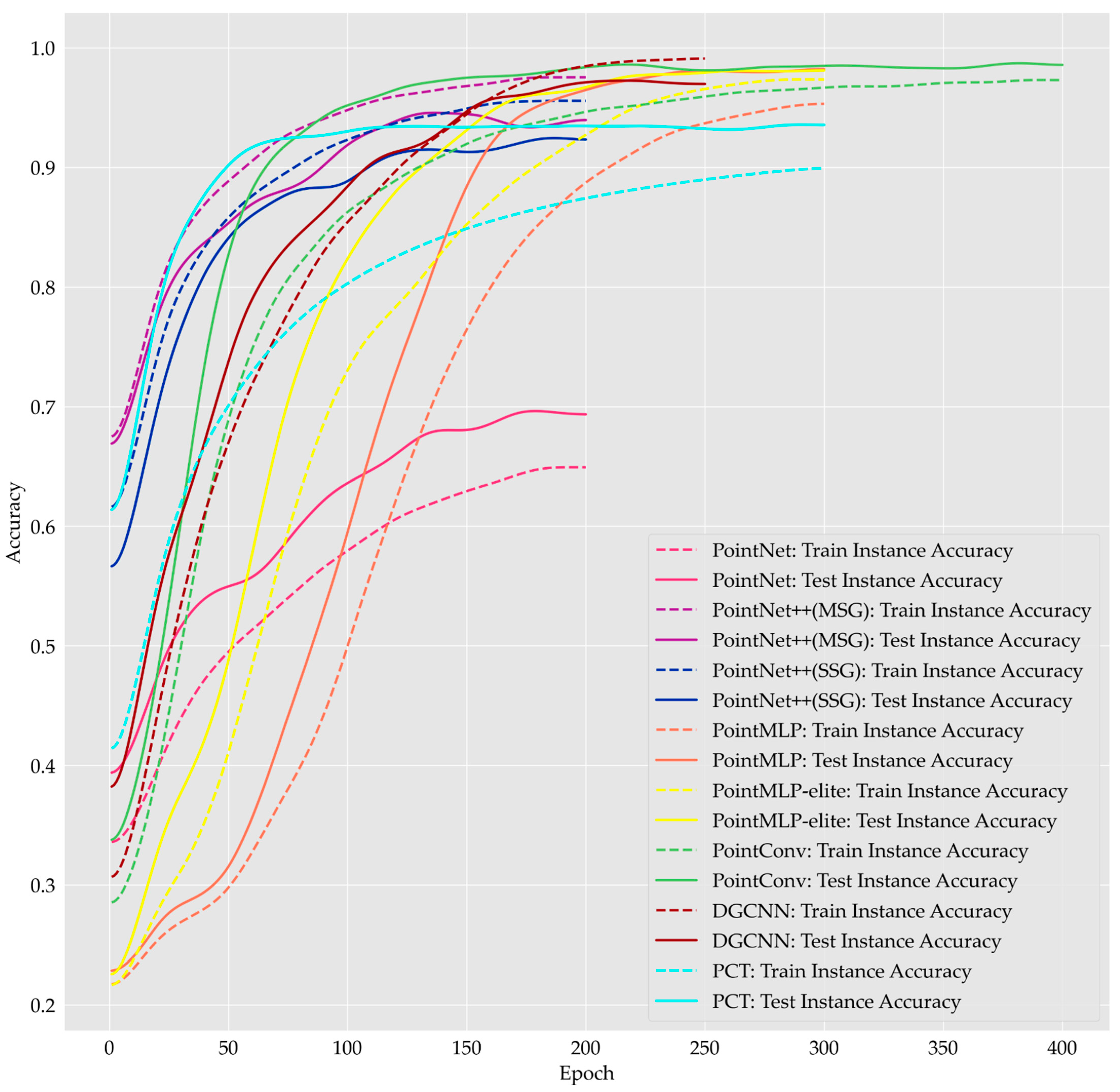
We recorded the change in training accuracy (Figure 5) and the change in loss (Figure 6) during the training of each deep learning model. Figure 5 shows that the improvement in training and testing accuracy for the PointNet model with increasing epochs was not very large. The training and testing accuracies of all other models eventually reached values greater than 0.90. Although the training accuracy of the PCT model reached a stable interval early, its test accuracy increased slowly after reaching 0.80. The training accuracy of the two PointNet++ models was always greater than the testing accuracy during the training process. The training accuracy of the MSG models was consistently higher than that of the SSG models. During the training of the DGCNN model, the training accuracy and the testing accuracy were basically the same when the Epoch was in the range of 150, following which the testing accuracy was relatively lower than the training accuracy as the training continued. From the perspective of model training accuracy, DGCNN performed relatively poorly. In the later stage of model training, the training accuracy kept improving, but the testing accuracy did not show good performance. For all other models, the test accuracy was always greater than the training accuracy during the deep learning training process. The advantages of the lightweight PointMLP-elite model can be seen. During model training, the PointMLP-elite model achieved higher training accuracy faster than PointMLP, and the final training accuracy remained consistent. The testing accuracy of the PointMLP-elite model was also higher than that of the PointMLP model. PointConv displayed a unique advantage in test accuracy, reaching over 0.95 at the early stage of training (Epoch = 100). There was also some slower improvement in the accuracy of PointConv as the training continued. The PCT model obtained a relatively high testing accuracy at the beginning of training (Epoch = 50); however, after epoch 75, the test accuracy did not grow significantly, although the training accuracy increased.
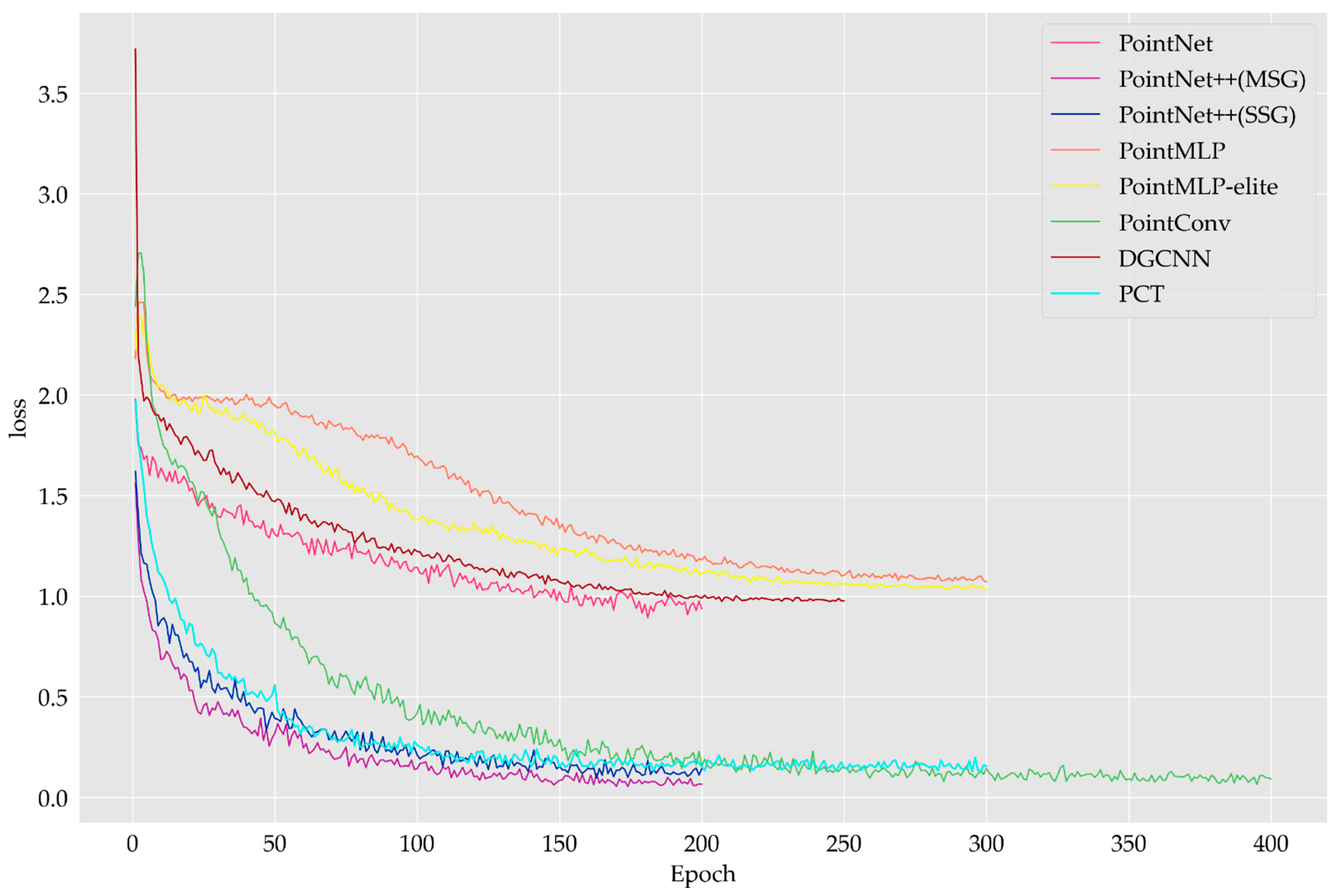
We could not evaluate different models exclusively with respect to the magnitude of the value of the loss, as different models use different processes for the calculation of the loss during the training of the model. However, we could compare models of the same type or models with the same loss processing method. Figure 6 shows that the loss of all the models decreased and eventually plateaued. This indicated that the training of all models was stable. PointNet and PointNet++ used the same model training strategy. The loss value of PointNet++ was eventually stable and close to 0, but the loss of the PointNet model was higher, with value stabilizing at approximately 1. This indicates that the classification performance of the PointNet model was worse than that of PointNet++. The loss values of the DGCNN and PointMLP models also finally stabilized at approximately 1.
4.2.2. Accuracy of Tree Species Classification
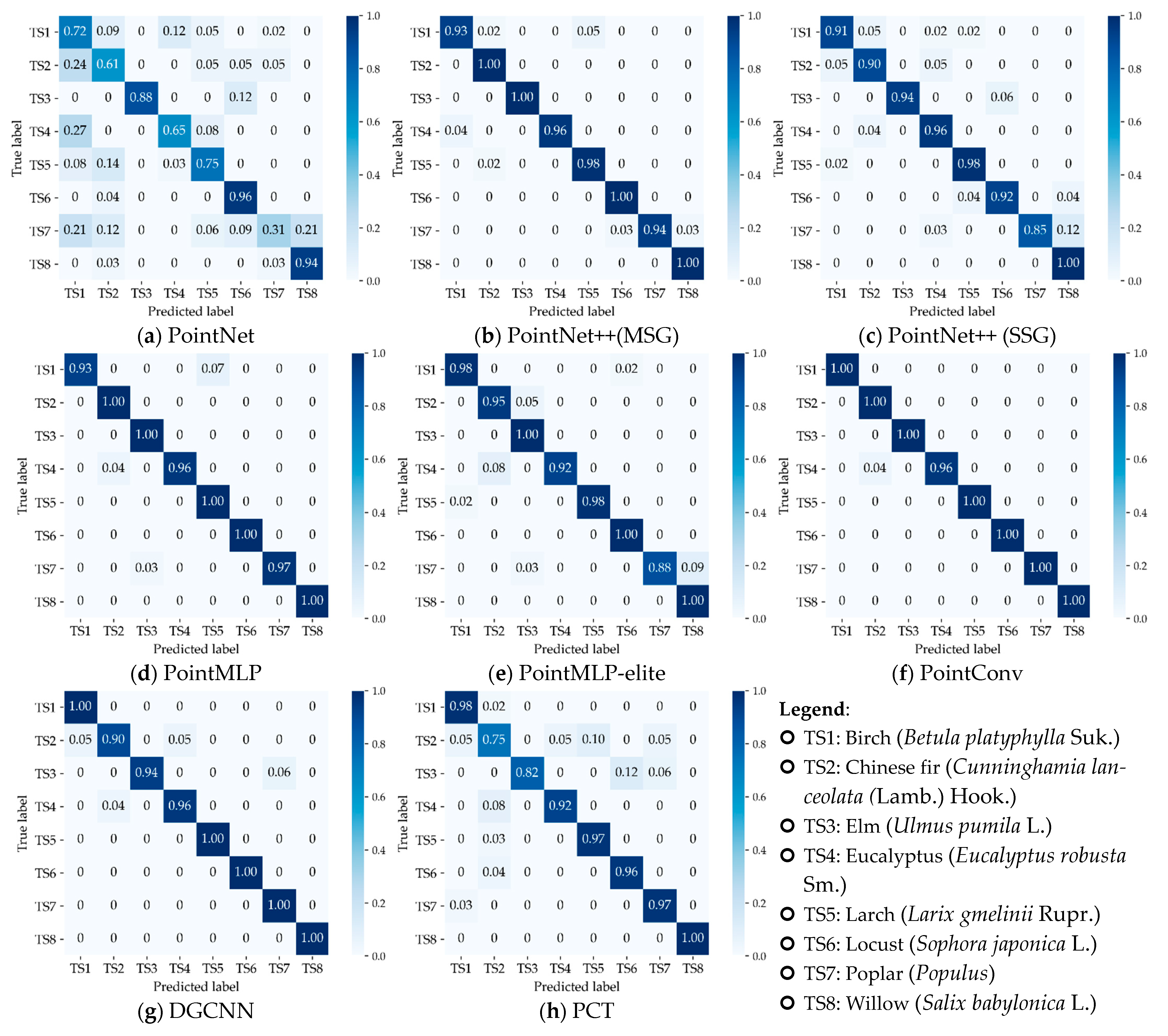
We summarize the final classification results of all models on the training and test sets and provide all model evaluation metrics in Table 3. As shown in the table, the PointNet model had the lowest evaluation metrics for all results. In the evaluation of the results on the test set, the PointConv model had the highest values in all evaluation metrics. As a recently proposed state-of-the-art (SOTA) pointwise MLP method, PointMLP ranked second in all classification evaluation metrics on the test set. The confusion matrices of the classification results for all models on the test data set are presented in Figure 7, which corroborate the results detailed in Table 3. The overall performance indicated that three models—PointConv, PointMLP, and DGCNN—classified all samples nearly completely correctly.
4.2.3. Model Comparison and Analysis
We summarize the values of some evaluation metrics, determined through a literature review, of the point cloud deep learning models used in this study in Table 4. The mean accuracy (mAcc) and overall accuracy (OA) in Table 4 denote the classification accuracies obtained from the deep learning models trained on the ModelNet40 data set. OA indicates the number of correct predictions as a percentage of the total number of samples, while mAcc indicates the arithmetic mean of accuracy for all categories. OA and mAcc correspond to the Re (or Acc) and BAcc evaluation metrics in the tree species classification experiments, respectively.
The structure and performance of point cloud deep learning models have been continuously improved and optimized by researchers, and newly proposed models have recently achieved higher classification accuracy. Among the experiments performed to classify the ModelNet40 data set, Table 4 shows that the PointMLP method had the highest classification accuracy, and three other methods—PointConv, DGCNN, and PCT—had similar classification accuracy. Meanwhile, the classification accuracies of PointNet and PointNet++ were lower. Furthermore, the PointMLP model had the largest number of parameters, while the elite version had the smallest number of parameters, and the difference in classification accuracy between the two models was small. The PointNet model had the second-highest number of parameters, but also had the worst classification accuracy. PointNet++ (MSG) had higher FLOPs and, thus, a higher computational burden. DGCNN and PCT had high classification accuracy but require a certain amount of memory and processor load on the computer.
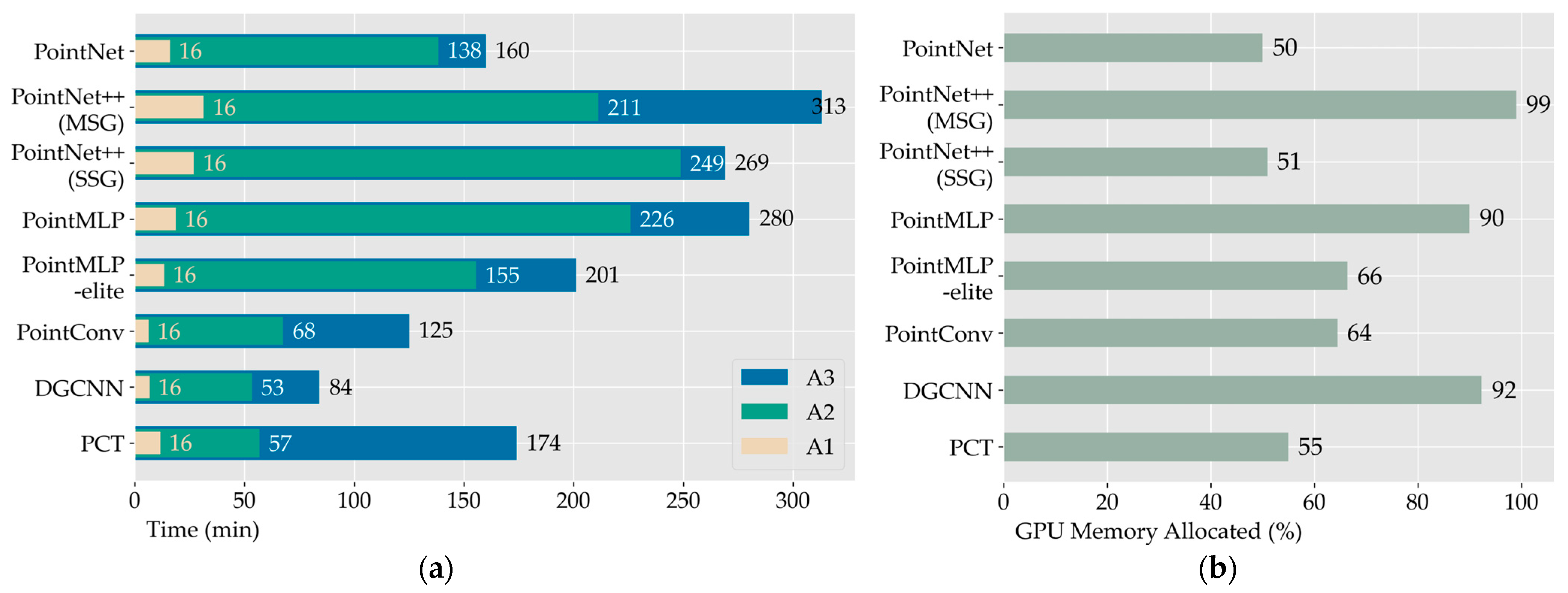
We counted the time spent for each model to train in the tree species classification experiment, which are plotted in Figure 8a, while Figure 8b displays the GPU memory occupancy of each model during training. As shown in Figure 8, the time required for training PointNet++ and PointMLP to obtain the optimal model parameters was longer. PointMLP-elite is a streamlined and lightweight version of PointMLP, with a model runtime reduction of 70 min, approximately 30% less than that of PointMLP. Using the same training parameters, the GPU memory of the PointMLP-elite model was reduced by 24%. Three models—PointConv, DGCNN, and PCT—took less time for training, but DGCNN had a higher GPU memory allocation.
4.3. Visualization of Critical Points
We extracted the critical points used for classification after training seven models, including PointNet, PointNet++ (MSG), PointNet++ (SSG), PointMLP, PointMLP-elite, DGCNN, and PCT, and selected samples of some tree species as cases for demonstration (Figure S1). Figure S1 shows that all critical points summarized the structure of the 3D objects well. Some tree species with similar shapes or structures will lead to misclassification, but this is rare.
5. Discussion
In this study, we demonstrated that four different point cloud deep learning model techniques, including pointwise MLP, convolution-based, graph-based, and attention-based models, perform well when categorizing tree species from individual tree LiDAR point clouds. We suggested a new approach for downsampling point clouds that combines the non-uniform grid and farthest point sampling methods. For training and testing experiments involving tree species categorization, we explored eight point cloud deep learning models: PointNet, PointNet++ (MSG), PointNet++ (SSG), PointMLP, PointMLP-elite, PointConv, DGCNN, and PCT. With the exception of PointNet, the accuracy of tree species classification for all models was greater than 90%. We extracted and visualized the set of critical points in feature convergence for each model when classifying each sample, which were found to comprehensively summarize the skeletons of the 3D point cloud object shapes.
Individual tree species point cloud data processed with the NGFPS method can be utilized to gain higher accuracy in tree species classification as it combines the non-uniform grid sampling and farthest point sampling algorithms. Using non-uniform grid sampling can preserve the details of 3D objects well, while FPS is a distance-based fast sampling method that guarantees uniform sampling, which has been widely used. The NGFPS combines the advantages of both of these downsampling methods and can represent the structure of 3D objects comprehensively and accurately.
The classification accuracy of the PointNet model was poor. This was because PointNet only considers the global features of the samples and ignores local features. Trees are usually grouped into one category in 3D object classification studies because their shape characteristics are very similar. Local detailed features are the key information necessary for classification when distinguishing different species of trees. The PointNet model cannot capture the local structure generated by the metric space points, thus limiting its ability to identify fine-grained patterns. All of the other five methods could extract the local feature information of 3D objects and achieved a higher classification accuracy.
The PointConv model achieved the highest classification accuracy and also required less training time. In 2D images, convolutional neural networks have fundamentally changed the landscape of computer vision by dramatically improving the results of almost all vision tasks [33]. Our experiments demonstrated the scalability of convolution-based point cloud deep learning models for the task of classifying 3D objects. The 3D convolutional deep learning method with local information extraction capability can successfully capture the structural features of trees for classification and recognition. Convolution plays a unique role in the study of deep learning.
The PointMLP model achieved a classification accuracy second only to that of the PointConv model, in terms of tree species classification. This confirmed that the existing feature extractors proposed by Ma et al. [24] can already describe the local geometric features of 3D objects well. More complex designs no longer need to be designed to further improve performance. This illustrates that we need to re-think and re-design algorithms for local feature extraction, in order to propose simple model structures for point cloud data analysis. The experimental results of the PointMLP-elite model illustrated that a simple deep learning model structure can still achieve good classification accuracy.
The PCT model did not achieve optimal classification accuracy in the tree species classification experiments. The transformer does not use recurrent neural layers, but attention mechanisms, which have a high degree of parallelism. However, attention mechanisms make fewer assumptions about the whole model, meaning that the transformer model has less adjustable parameters, which leads to a need for more data and a larger model to train in order to achieve the same effect as a CNN [48]. In this experiment, the final classification accuracy is relatively low because the samples used for deep learning model training are relatively small. This is why transformer-based models are considered to be larger and more expensive. The transformer is a feature extraction method based on an attention mechanism, which was originally proposed for natural language translation. However, scholars have found that the model can be applied in any deep learning domain. Transformers can fuse various data, such as text, images, speech, video, and so on, and extract features within one and the same framework as a means to train larger and better models. This is a hotspot and focus of deep learning research at present and is expected to remain so for some time.
The ranking of OA on the ModelNet40 dataset differs from the results of the tree species classification experiments for different models. The results in Table 3 and Table 4 show that, although the recently developed models (PointMLP, PCT) achieved superior classification accuracy in experiments on 3D object classification, the convolution-based method (PointConv) and the MLP-based method (PointNet++ (MSG)) had higher classification accuracy when performing tree species identification on individual tree point clouds. This indicates that more models and methods need to be considered for use in different classification tasks of 3D objects. The evaluation of the number of parameters and performance of different models need to be reanalyzed for different experimental tasks.
Our experiments still had several flaws that will need to be addressed in the future. Due to the small number of training examples, transformer, a promising deep learning framework at the moment, did not demonstrate its advantages in this study. In future related works, we hope to broaden the application of transformer models in point cloud deep learning by extending the amount of data to as many samples as possible. Similar to the authenticity test of remote sensing products [49,50,51], we must reduce the error tolerance of training samples while improving the accuracy of the model by drawing on the authenticity test. It has been proposed that very high-accuracy models can be trained using MLP or simpler architectures; however, we found that the training time of pointwise MLP-based methods was higher than that of other types of methods. The scalability of the deep learning models used at this stage must be further demonstrated through various experiments, as the methods currently designed and developed by scholars have been proposed based on several data sets common to the field of computer vision. In this context, more architectures are sure to emerge and expand into more research areas in the future.
Overall, our experiment was very successful. The NGFPS method can aid in deep learning model training, obtaining higher accuracies, and different types of point cloud deep learning methods were shown to achieve good results in the study of tree species classification. The proposal of new point cloud deep learning methods, such as PointMLP, provides us with more options in the study of tree species classification.
6. Conclusions
Deep learning approaches were demonstrated to be capable of identifying individual tree point cloud species very accurately. The NGFPS method, which combines the non-uniform grid and farthest point sampling methods, can better preserve the details and structural information of 3D objects, providing accurate data input for deep learning models to accurately identify the features of different tree species. All deep learning models generalized the classification objects in terms of both local and global features. In particular, the convolution-based PointConv model exemplified its superior performance for 3D object classification. Furthermore, deep learning algorithms need not be more complex than they currently are, as the lightweight PointMLP-elite model presented unique advantages over PointMLP. The PointNet++ model, a foundational model for point-based deep learning methods, still exhibited high classification accuracy in tree species classification studies. Point cloud deep learning models are constantly developing, and the potentials of deep learning techniques will be continuously explored. The successful practice of using deep learning models for individual tree species classification provides a new solution, allowing for more efficient forest resource surveys.
Supplementary Materials
The following supporting information can be downloaded at: https://www.mdpi.com/article/10.3390/rs14225733/s1, Figure S1: Visualization of Critical Points.
Author Contributions
Conceptualization, X.T. and B.L.; methodology, B.L.; software, B.L., S.C. and Y.S.; validation, B.L. and Y.S.; formal analysis, B.L. and Y.S.; investigation, B.L., S.C. and Y.S.; resources, X.T., Z.L. and E.C.; data curation, B.L.; writing—original draft preparation, B.L. and X.T.; writing—review and editing, H.H., Z.L. and E.C.; visualization, B.L. and S.C.; supervision, H.H., Z.L. and E.C.; project administration, X.T. and H.H.; funding acquisition, X.T. and H.H. All authors have read and agreed to the published version of the manuscript.
Funding
This research was funded by the Cooperation Project Between Zhejiang Province and Chinese Academy of Forestry in Forestry Science and Technology (Grant number: 2020SY02), the National Science and Technology Major Project of China’s High Resolution Earth Observation System (Grant number: 21-Y20B01-9001-19/22), the National Natural Science Foundation of China (Grant number: 42130111 and 41930111), the National Key Research and Development Program of China (Grant number: 2021YFE0117700), the National Natural Science Foundation of China (Grant number: 41871279), and the Fundamental Research Funds of CAF (Grant number: CAFYBB2021SY006).
Data Availability Statement
Not applicable.
Acknowledgments
We are grateful to Chao Ma and Qiuyi Ai for their help in field data collection.
Conflicts of Interest
The authors declare no conflict of interest.
References
- Schiefer, F.; Kattenborn, T.; Frick, A.; Frey, J.; Schall, P.; Koch, B.; Schmidtlein, S. Mapping forest tree species in high resolution UAV-based RGB-imagery by means of convolutional neural networks. ISPRS J. Photogramm. Remote Sens. 2020, 170, 205–215. [Google Scholar] [CrossRef]
- Crabbe, R.A.; Lamb, D.; Edwards, C. Discrimination of species composition types of a grazed pasture landscape using Sentinel-1 and Sentinel-2 data. Int. J. Appl. Earth Obs. Geoinf. 2020, 84, 101978. [Google Scholar] [CrossRef]
- Torabzadeh, H.; Leiterer, R.; Hueni, A.; Schaepman, M.E.; Morsdorf, F. Tree species classification in a temperate mixed forest using a combination of imaging spectroscopy and airborne laser scanning. Agric. For. Meteorol. 2019, 279, 107744. [Google Scholar] [CrossRef]
- Liu, J.; Wang, X.; Wang, T. Classification of tree species and stock volume estimation in ground forest images using Deep Learning. Comput. Electron. Agric. 2019, 166, 105012. [Google Scholar] [CrossRef]
- Pu, R. Mapping Tree Species Using Advanced Remote Sensing Technologies: A State-of-the-Art Review and Perspective. J. Remote Sens. 2021, 2021, 812624. [Google Scholar] [CrossRef]
- Briechle, S.; Krzystek, P.; Vosselman, G. Semantic Labeling of Als Point Clouds for Tree Species Mapping Using the Deep Neural Network Pointnet++. Int. Arch. Photogramm. Remote Sens. Spat. Inf. Sci. 2019, XLII-2/W13, 951–955. [Google Scholar] [CrossRef] [Green Version]
- Briechle, S.; Krzystek, P.; Vosselman, G. Classification of Tree Species and Standing Dead Trees by Fusing Uav-Based Lidar Data and Multispectral Imagery in the 3d Deep Neural Network Pointnet++. ISPRS Ann. Photogramm. Remote Sens. Spat. Inf. Sci. 2020, V-2-2020, 203–210. [Google Scholar] [CrossRef]
- Liu, M.; Han, Z.; Chen, Y.; Liu, Z.; Han, Y. Tree species classification of LiDAR data based on 3D deep learning. Measurement 2021, 177, 109301. [Google Scholar] [CrossRef]
- Lv, Y.; Zhang, Y.; Dong, S.; Yang, L.; Zhang, Z.; Li, Z.; Hu, S. A Convex Hull-Based Feature Descriptor for Learning Tree Species Classification from ALS Point Clouds. IEEE Geosci. Remote Sens. Lett. 2022, 19, 1–5. [Google Scholar] [CrossRef]
- Seidel, D.; Annighofer, P.; Thielman, A.; Seifert, Q.E.; Thauer, J.H.; Glatthorn, J.; Ehbrecht, M.; Kneib, T.; Ammer, C. Predicting Tree Species From 3D Laser Scanning Point Clouds Using Deep Learning. Front. Plant Sci. 2021, 12, 635440. [Google Scholar] [CrossRef]
- Xi, Z.; Hopkinson, C.; Rood, S.B.; Peddle, D.R. See the forest and the trees: Effective machine and deep learning algorithms for wood filtering and tree species classification from terrestrial laser scanning. ISPRS J. Photogramm. Remote Sens. 2020, 168, 1–16. [Google Scholar] [CrossRef]
- Su, Y.; Guo, Q.; Jin, S.; Guan, H.; Sun, X.; Ma, Q.; Hu, T.; Wang, R.; Li, Y. The Development and Evaluation of a Backpack LiDAR System for Accurate and Efficient Forest Inventory. IEEE Geosci. Remote Sens. Lett. 2021, 18, 1660–1664. [Google Scholar] [CrossRef]
- Guan, H.; Yu, Y.; Ji, Z.; Li, J.; Zhang, Q. Deep learning-based tree classification using mobile LiDAR data. Remote Sens. Lett. 2015, 6, 864–873. [Google Scholar] [CrossRef]
- Liu, B.; Chen, S.; Huang, H.; Tian, X. Tree Species Classification of Backpack Laser Scanning Data Using the PointNet++ Point Cloud Deep Learning Method. Remote Sens. 2022, 14, 3809. [Google Scholar] [CrossRef]
- Zou, X.; Cheng, M.; Wang, C.; Xia, Y.; Li, J. Tree Classification in Complex Forest Point Clouds Based on Deep Learning. IEEE Geosci. Remote Sens. Lett. 2017, 14, 2360–2364. [Google Scholar] [CrossRef]
- Wan, H.; Tang, Y.; Jing, L.; Li, H.; Qiu, F.; Wu, W. Tree Species Classification of Forest Stands Using Multisource Remote Sensing Data. Remote Sens. 2021, 13, 144. [Google Scholar] [CrossRef]
- Åkerblom, M.; Raumonen, P.; Mäkipää, R.; Kaasalainen, M. Automatic tree species recognition with quantitative structure models. Remote Sens. Environ. 2017, 191, 1–12. [Google Scholar] [CrossRef]
- Ba, A.; Laslier, M.; Dufour, S.; Hubert-Moy, L. Riparian trees genera identification based on leaf-on/leaf-off airborne laser scanner data and machine learning classifiers in northern France. Int. J. Remote Sens. 2019, 41, 1645–1667. [Google Scholar] [CrossRef]
- Lin, Y.; Herold, M. Tree species classification based on explicit tree structure feature parameters derived from static terrestrial laser scanning data. Agric. For. Meteorol. 2016, 216, 105–114. [Google Scholar] [CrossRef]
- Yang, G.; Zhao, Y.; Li, B.; Ma, Y.; Li, R.; Jing, J.; Dian, Y. Tree Species Classification by Employing Multiple Features Acquired from Integrated Sensors. J. Sens. 2019, 2019, 3247946. [Google Scholar] [CrossRef]
- Budei, B.C.; St-Onge, B.; Hopkinson, C.; Audet, F.-A. Identifying the genus or species of individual trees using a three-wavelength airborne lidar system. Remote Sens. Environ. 2018, 204, 632–647. [Google Scholar] [CrossRef]
- Liu, L.; Coops, N.C.; Aven, N.W.; Pang, Y. Mapping urban tree species using integrated airborne hyperspectral and LiDAR remote sensing data. Remote Sens. Environ. 2017, 200, 170–182. [Google Scholar] [CrossRef]
- Yu, X.; Hyyppä, J.; Litkey, P.; Kaartinen, H.; Vastaranta, M.; Holopainen, M. Single-Sensor Solution to Tree Species Classification Using Multispectral Airborne Laser Scanning. Remote Sens. 2017, 9, 108. [Google Scholar] [CrossRef] [Green Version]
- Ma, X.; Qin, C.; You, H.; Ran, H.; Fu, Y. Rethinking Network Design and Local Geometry in Point Cloud: A Simple Residual MLP Framework. In Proceedings of the International Conference on Learning Representations (ICLR), Virtual Event, 25–29 April 2022. [Google Scholar]
- Qi, C.R.; Su, H.; Mo, K.; Guibas, L.J. Pointnet: Deep learning on point sets for 3d classification and segmentation. In Proceedings of the IEEE Conference on Computer Vision and Pattern Recognition, Honolulu, HI, USA, 21–26 July 2017; pp. 652–660. [Google Scholar]
- Qi, C.R.; Yi, L.; Su, H.; Guibas, L.J. Pointnet++: Deep hierarchical feature learning on point sets in a metric space. In Proceedings of the 30th Annual Conference on Neural Information Processing Systems Conference (NIPS 2017), Long Beach, CA, USA, 4–9 December 2017; Volume 30. [Google Scholar]
- Guo, Y.; Wang, H.; Hu, Q.; Liu, H.; Liu, L.; Bennamoun, M. Deep Learning for 3D Point Clouds: A Survey. IEEE Trans. Pattern Anal. Mach. Intell. 2021, 43, 4338–4364. [Google Scholar] [CrossRef]
- Wang, W.; Li, L. Review of Deep Learning in Point Cloud Classification. Comput. Eng. Appl. 2022, 58, 26–40. [Google Scholar] [CrossRef]
- Ge, L.; Yang, Z.; Sun, Z.; Zhang, G.; Zhang, M.; Zhang, K.; Zhang, C.; Tan, Y.; Li, W. A Method for Broccoli Seedling Recognition in Natural Environment Based on Binocular Stereo Vision and Gaussian Mixture Model. Sensors 2019, 19, 1132. [Google Scholar] [CrossRef] [Green Version]
- Zhou, B.; Khosla, A.; Lapedriza, A.; Oliva, A.; Torralba, A. Learning Deep Features for Discriminative Localization. In Proceedings of the IEEE Conference on Computer Vision and Pattern Recognition (CVPR), Las Vegas, NV, USA, 27–30 June 2016; pp. 2921–2929. [Google Scholar]
- Angelov, P.P.; Soares, E.A.; Jiang, R.; Arnold, N.I.; Atkinson, P.M. Explainable artificial intelligence: An analytical review. WIREs Data Min. Knowl. Discov. 2021, 11, e1424. [Google Scholar] [CrossRef]
- Huang, S.; Zhang, B.; Shen, W.; Wei, Z. A claim approach to understanding the pointnet. In Proceedings of the International Conference on Algorithms, Computing and Artificial Intelligence, Sanya, China, 20–22 December 2019; pp. 97–103. [Google Scholar]
- Wu, W.; Qi, Z.; Fuxin, L. PointConv: Deep Convolutional Networks on 3D Point Clouds. In Proceedings of the IEEE/CVF Conference on Computer Vision and Pattern Recognition (CVPR), Long Beach, CA, USA, 16–20 June 2019; pp. 9621–9630. [Google Scholar]
- Wang, Y.; Sun, Y.; Liu, Z.; Sarma, S.E.; Bronstein, M.M.; Solomon, J.M. Dynamic Graph CNN for Learning on Point Clouds. ACM Trans. Graph. 2019, 38, 1–12. [Google Scholar] [CrossRef] [Green Version]
- Guo, M.; Cai, J.; Liu, Z.; Mu, T.; Martin, R.R.; Hu, S. PCT: Point cloud transformer. Comput. Vis. Media 2021, 7, 187–199. [Google Scholar] [CrossRef]
- Zhang, W.; Qi, J.; Wan, P.; Wang, H.; Xie, D.; Wang, X.; Yan, G. An Easy-to-Use Airborne LiDAR Data Filtering Method Based on Cloth Simulation. Remote Sens. 2016, 8, 501. [Google Scholar] [CrossRef]
- Tao, S.; Wu, F.; Guo, Q.; Wang, Y.; Li, W.; Xue, B.; Hu, X.; Li, P.; Tian, D.; Li, C.; et al. Segmenting tree crowns from terrestrial and mobile LiDAR data by exploring ecological theories. ISPRS J. Photogramm. Remote Sens. 2015, 110, 66–76. [Google Scholar] [CrossRef] [Green Version]
- Wu, Z.; Song, S.; Khosla, A.; Yu, F.; Zhang, L.; Tang, X.; Xiao, J. 3D ShapeNets: A deep representation for volumetric shapes. In Proceedings of the IEEE Conference on Computer Vision and Pattern Recognition, Boston, MA, USA, 7–12 June 2015; pp. 1912–1920. [Google Scholar]
- Pomerleau, F.; Colas, F.; Siegwart, R.; Magnenat, S. Comparing ICP variants on real-world data sets. Auton. Robot. 2013, 34, 133–148. [Google Scholar] [CrossRef]
- Lee, K.H.; Woo, H.; Suk, T. Point Data Reduction Using 3D Grids. Int. J. Adv. Manuf. Technol. 2001, 18, 201–210. [Google Scholar] [CrossRef]
- Mo, K.; Yin, Z. Surface Reconstruction of Defective Point Clouds Based on Dual Off-Set Gradient Functions. In Advances in Mechatronics; IntechOpen: Rijeka, Croatia, 2011. [Google Scholar]
- Zhao, S.; Li, F.; Liu, Y.; Rao, Y. A New Method for Cloud Data Reduction Using Uniform Grids. In Proceedings of the 2013 International Conference on Advanced Computer Science and Electronics Information (ICACSEI 2013), Beijing, China, 25–26 July 2013; pp. 64–67. [Google Scholar]
- Fan, S.; Dong, Q.; Zhu, F.; Lv, Y.; Ye, P.; Wang, F. SCF-Net: Learning Spatial Contextual Features for Large-Scale Point Cloud Segmentation. In Proceedings of the IEEE/CVF Conference on Computer Vision and Pattern Recognition, Nashville, TN, USA, 19–25 June 2021; pp. 14504–14513. [Google Scholar]
- Xu, M.; Ding, R.; Zhao, H.; Qi, X. PAConv: Position Adaptive Convolution With Dynamic Kernel Assembling on Point Clouds. In Proceedings of the IEEE/CVF Conference on Computer Vision and Pattern Recognition, Nashville, TN, USA, 19–25 June 2021; pp. 3173–3182. [Google Scholar]
- Zhao, H.; Jiang, L.; Jia, J.; Torr, P.H.S.; Koltun, V. Point Transformer. In Proceedings of the IEEE/CVF International Conference on Computer Vision, Montreal, BC, Canada, 11–17 October 2021; pp. 16259–16268. [Google Scholar]
- Engel, N.; Belagiannis, V.; Dietmayer, K. Point Transformer. IEEE Access 2021, 9, 134826–134840. [Google Scholar] [CrossRef]
- Cheng, X.; Doosthosseini, A.; Kunkel, J. Improve the Deep Learning Models in Forestry Based on Explanations and Expertise. Front. Plant Sci. 2022, 13, 902105. [Google Scholar] [CrossRef]
- Liu, Y.; Sangineto, E.; Bi, W.; Sebe, N.; Lepri, B.; Nadai, M.D. Efficient Training of Visual Transformers with Small Datasets. In Proceedings of the 35th Conference on Neural Information Processing Systems, Virtual Conference, 7–10 December 2021. [Google Scholar]
- Wen, J.; Wu, X.; Wang, J.; Tang, R.; Ma, D.; Zeng, Q.; Gong, B.; Xiao, Q. Characterizing the Effect of Spatial Heterogeneity and the Deployment of Sampled Plots on the Uncertainty of Ground “Truth” on a Coarse Grid Scale: Case Study for Near-Infrared (NIR) Surface Reflectance. J. Geophys. Res. Atmos. 2022, 127, e2022JD036779. [Google Scholar] [CrossRef]
- Wen, J.; You, D.; Han, Y.; Lin, X.; Wu, S.; Tang, Y.; Xiao, Q.; Liu, Q. Estimating Surface BRDF/Albedo Over Rugged Terrain Using an Extended Multisensor Combined BRDF Inversion (EMCBI) Model. IEEE Geosci. Remote Sens. Lett. 2022, 19, 1–5. [Google Scholar] [CrossRef]
- Wu, X.; Wen, J.; Xiao, Q.; Bao, Y.; You, D.; Wang, J.; Ma, D.; Lin, X.; Gong, B. Quantification of the Uncertainty Caused by Geometric Registration Errors in Multiscale Validation of Satellite Products. IEEE Geosci. Remote Sens. Lett. 2022, 19, 1–5. [Google Scholar] [CrossRef]
Figure 1.
Distribution map of the study area and some of the LiDAR data collected in the field.

Figure 2.
An overview of the workflow for individual tree point cloud-based tree species classification.
Figure 2.
An overview of the workflow for individual tree point cloud-based tree species classification.

Figure 3.
Model structure visualization of six considered point cloud deep learning models.

Figure 4.
Model evaluation metrics for FPS and NGFPS on test data sets.

Figure 5.
The change of training accuracy and testing accuracy for all models during the training process (we performed Gaussian smoothing on the y-value of each curve, where the smoothing parameter was set to 10).
Figure 5.
The change of training accuracy and testing accuracy for all models during the training process (we performed Gaussian smoothing on the y-value of each curve, where the smoothing parameter was set to 10).

Figure 6.
Changes in loss function during model training.

Figure 7.
Confusion matrices of the classification results on the test set for all models.

Figure 8.
Model training time and GPU memory usage: (a) Model training time. A1 denotes the time required for each epoch (which we have expanded by a factor of 20 for presentation purposes). A2 denotes the time required for training to obtain the optimal model. A3 denotes the total duration of the model operation; and (b) Occupancy of GPU memory.


Table 1.
Study area and tree species information.
| Study Area | Location | Plot Size | Tree Species | Genus | Tree Height (m) | Number |
|---|---|---|---|---|---|---|
| GKS | 120°12′ to 122°55′ E, 50°20′ to 52°30′ N | 25 m × 25 m | Birch (Betula platyphylla Suk.) | Betula | 6.58–20.87 | 215 |
| Larch (Larix gmelinii Rupr.) | Larix | 6.23–19.30 | 295 | |||
| HL | 115°47′ E, 40°20′ N | 20 m × 20 m | Locust (Styphnolobium japonicum L.) | Styphnolobium | 4.91–9.79 | 142 |
| Willow (Salix babylonica L.) | Salix | 6.33–12.55 | 174 | |||
| Poplar (Populus L.) | Populus | 14.39–25.04 | 165 | |||
| Elm (Ulmus pumila L.) | Ulmus | 4.37–13.48 | 85 | |||
| GF | 108°20′ to 108°32′ E, 22°56′ to 23°4′ N | 20 m × 20 m | Eucalyptus (Eucalyptus robusta Sm.) | Eucalyptus | 20.34–34.66 | 131 |
| Chinese fir (Cunninghamia lanceolata (Lamb.) Hook.) | Cunninghamia | 7.51–22.64 | 105 |
Table 2.
Hyperparameters used in the training process of six point cloud deep learning models.
| Category | Pointwise MLP | Convolution | Graph | Attention | ||
|---|---|---|---|---|---|---|
| Model | PointNet | PointNet++ | PointMLP | PointConv | DGCNN | PCT |
| Batch Size | 12 | 12 | 12 | 12 | 8 | 12 |
| Number of Points | 2048 | 2048 | 2048 | 2048 | 2048 | 2048 |
| Number of Categories | 8 | 8 | 8 | 8 | 8 | 8 |
| Epochs | 200 | 200 | 300 | 400 | 250 | 300 |
| Optimizer | Adam | Adam | SGD | SGD | SGD | Adam |
| Learning Rate | 0.001 | 0.001 | 0.1 | 0.01 | 0.1 | 0.0001 |
| Weight Decay | 0.0001 | 0.0001 | 0.0002 | — | 0.0001 | 0.0001 |
| Momentum | — | — | 0.9 | 0.9 | 0.9 | — |
| Learning Rate Scheduler 1 | StepLR | StepLR | CosineAnnealingLR | StepLR | CosineAnnealingLR | StepLR |
| Loss Function 2 | NLLLOSS | NLLLOSS | CrossEntropyLoss | NLLLOSS | CrossEntropyLoss | CrossEntropyLoss |
| Activation Function | ReLU and LogSoftmax | ReLU and LogSoftmax | ReLU and AdaptiveMaxPool1d | ReLU and LogSoftmax | LeakyReLU and AdaptiveMaxPool1d + AdaptiveAvgPool1d | ReLU and Max |
1 Learning Rate Scheduler: StepLR: Decay the learning rate of each parameter group by gamma every epoch (https://pytorch.org/docs/stable/generated/torch.optim.lr_scheduler.StepLR.html, accessed on 2 November 2022). CosineAnnealingLR: Set the learning rate of each parameter group using a cosine annealing schedule (https://pytorch.org/docs/stable/generated/torch.optim.lr_scheduler.CosineAnnealingLR.html, accessed on 2 November 2022). 2 Loss Function: NLLLOSS: The negative log-likelihood loss (https://pytorch.org/docs/stable/generated/torch.nn.NLLLoss.html, accessed on 2 November 2022). CrossEntropyLoss: Cross entropy loss (https://pytorch.org/docs/stable/generated/torch.nn.CrossEntropyLoss.html, accessed on 2 November 2022).
Table 3.
Evaluation metrics for model classification results.
| Model | BAcc | Pr | Re | F | kappa | |||||
|---|---|---|---|---|---|---|---|---|---|---|
| Train | Test | Train | Test | Train | Test | Train | Test | Train | Test | |
| PointNet | 0.6251 | 0.7288 | 0.6277 | 0.7492 | 0.6351 | 0.7241 | 0.6288 | 0.7183 | 0.5726 | 0.679 |
| PointNet++(MSG) | 0.9642 | 0.9768 | 0.9648 | 0.974 | 0.9646 | 0.9732 | 0.9645 | 0.9731 | 0.9587 | 0.9687 |
| PointNet++(SSG) | 0.9579 | 0.9343 | 0.9579 | 0.9421 | 0.9579 | 0.9387 | 0.9578 | 0.9387 | 0.9508 | 0.9284 |
| PointMLP | 0.9097 | 0.9827 | 0.931 | 0.9818 | 0.9301 | 0.9808 | 0.9294 | 0.9808 | 0.9181 | 0.9776 |
| PointMLP-elite | 0.9467 | 0.9643 | 0.9562 | 0.9677 | 0.955 | 0.9655 | 0.955 | 0.9655 | 0.9473 | 0.9598 |
| PointConv | 0.9432 | 0.9952 | 0.9507 | 0.9963 | 0.9505 | 0.9962 | 0.9505 | 0.9962 | 0.9423 | 0.9955 |
| DGCNN | 0.9759 | 0.9614 | 0.9847 | 0.9648 | 0.9847 | 0.9647 | 0.9845 | 0.9647 | 0.9821 | 0.9588 |
| PCT | 0.9321 | 0.9232 | 0.9343 | 0.9441 | 0.9343 | 0.9425 | 0.9342 | 0.9426 | 0.9234 | 0.9329 |
The numbers in bold represent the maximum values of the indicators in each column.
Table 4.
Results for all models trained on the ModelNet40 data set.
| Model | Year | mAcc | OA | #Params | #FLOPs | Ref. |
|---|---|---|---|---|---|---|
| PointNet | 2017 | 0.860 | 0.892 | 3.47 M | 0.45 G | [25] |
| PointNet++(MSG) | 2017 | — | 0.919 | 1.74 M | 4.09 G | [26] |
| PointNet++(SSG) | 2017 | — | 0.907 | 1.48 M | 1.68 G | [26] |
| PointMLP | 2022 | 0.914 | 0.945 | 12.6 M | — | [24] |
| PointMLP-elite | 2022 | 0.907 | 0.940 | 0.68 M | — | [24] |
| PointConv | 2018 | — | 0.925 | — | — | [33] |
| DGCNN | 2019 | 0.902 | 0.929 | 1.81 M | 2.43 G | [34] |
| PCT | 2021 | — | 0.932 | 2.88 M | 2.32 G | [35] |
#Params indicate the number of parameters required by the model; #FLOPs indicate the number of floating-point operations for the model.
Publisher’s Note: MDPI stays neutral with regard to jurisdictional claims in published maps and institutional affiliations. |
© 2022 by the authors. Licensee MDPI, Basel, Switzerland. This article is an open access article distributed under the terms and conditions of the Creative Commons Attribution (CC BY) license (https://creativecommons.org/licenses/by/4.0/).
Share and Cite
MDPI and ACS Style
Liu, B.; Huang, H.; Su, Y.; Chen, S.; Li, Z.; Chen, E.; Tian, X. Tree Species Classification Using Ground-Based LiDAR Data by Various Point Cloud Deep Learning Methods. Remote Sens. 2022, 14, 5733. https://doi.org/10.3390/rs14225733
AMA Style
Liu B, Huang H, Su Y, Chen S, Li Z, Chen E, Tian X. Tree Species Classification Using Ground-Based LiDAR Data by Various Point Cloud Deep Learning Methods. Remote Sensing. 2022; 14(22):5733. https://doi.org/10.3390/rs14225733
Chicago/Turabian StyleLiu, Bingjie, Huaguo Huang, Yong Su, Shuxin Chen, Zengyuan Li, Erxue Chen, and Xin Tian. 2022. "Tree Species Classification Using Ground-Based LiDAR Data by Various Point Cloud Deep Learning Methods" Remote Sensing 14, no. 22: 5733. https://doi.org/10.3390/rs14225733
Note that from the first issue of 2016, this journal uses article numbers instead of page numbers. See further details here.