Article

The Temporal Evolution of Coastlines in the Bohai Sea and Its Impact on Hydrodynamics

1
Frontier Science Center for Deep Ocean Multispheres and Earth System (FDOMES) and Physical Oceanography Laboratory, Ocean University of China, Qingdao 266100, China
2
First Institute of Oceanography, Ministry of Natural Resources, Qingdao 266061, China
3
Pilot National Laboratory for Marine Science and Technology, Qingdao 266237, China
*
Author to whom correspondence should be addressed.
Remote Sens. 2022, 14(21), 5549; https://doi.org/10.3390/rs14215549
Submission received: 26 September 2022 / Revised: 29 October 2022 / Accepted: 29 October 2022 / Published: 3 November 2022
(This article belongs to the Special Issue Remote Sensing and Numerical Simulation for Tidal Dynamics)

Abstract

:
Over the past 40 years, increasing coastal reclamation and natural sedimentation has changed coastline positions and resulted in variation in the hydrodynamic environment in the Bohai Sea (BHS), China. Based on the Landsat series images, an interpretative identifier for identifying the coastline was proposed to assess the hydrodynamic changes caused by the coastline change and was applied to a typical case of the Bohai Sea (BHS), China. We combined a grid-based coastline position with an adjoint data assimilation method to seamlessly map the distribution of the amplitude, phase lag, and tidal current of the M2 tidal constituent along the BHS’s coast from 1985 to 2018. Our findings reveal that the coastline change at long time scales dominated reclamation, and around 72.9% of the coastline of the BHS mapped in 2018 had seaward movement compared with its position in 1985. From 1985 to 2018, the BHS volume decreased by 0.17%, the sea surface area decreased by 4.54%, and the kinetic energy increased by 2.53%. The change in the coastline increased the amplitude of the M2 tidal constituent in the Bohai Bay by 6–14 cm and increased the residual current in the eastern coast of the Liaodong Bay by up to 0.07 (0.01) m/s.

1. Introduction

A coastline is a physical boundary between land and water and provides a fundamental proxy to measure coastal variability and change [1]. However, multiple natural factors, including coastal erosion [2], coastal subsidence [3], and sea level rise [4], result in the spatially heterogeneous and complex change in coastlines [5]. In addition, the intensive human interferences, including mariculture pond [6], port [7], and bridge construction [8], can result in irreversible changes in coastal morphology and the loss of natural characteristics. The coastline changes induced by human interference not only directly modify the local morphology but also result in rapid changes in the hydrodynamic regime. Studies showed coastline change can alter the tidal current velocity [9,10], reduce the tidal prism [11], alter the water and salt transport processes [12], and result in tidal amplitude variations [13,14].
The Bohai Sea (BHS) is a semi-enclosed sea situated in Northeast China and may be described as a hotspot among the world’s marginal seas with respect to its large natural and anthropogenic coastline changes [15]. In recent years, the BHS has faced threats from large-scale development, reclamation, sea level rise, and coastal erosion. These threats will lead to a significant loss of coastal wetland and the degradation of natural coastline [16,17]. In particular, the Yellow River Estuary is well-known for its rapid erosion–deposition variation, which is caused by dramatic changes in river flows and ocean tides [10]. Consequently, the effect of the BHS’s environment due to coastline change has recently drawn special attention from many coastal scientists and managers [18]. A study confirmed that harbors, seawalls, industrial complexes, and urban districts constructed on the reclaimed land will permanently change the geomorphology of the coastline and the physical processes in the coastal system, resulting in more impacts on coastal hydrodynamics and sediment processes [9,10,19,20]. With the exploitation of the ocean, the study of the hydrodynamic variation caused by coastline change is much more important in coastal regions and marginal seas [21,22,23].
Previous numerical-simulation-based tidal studies have either explicitly or implicitly assumed that local shoreline positions have a negligible impact on tides in the BHS [24,25,26]. Coastline changes can effectively reduce or increase long-term temporal variability in tidal range, energy, and current velocity. Pelling et al. [15] investigated the effects of rapid coastline changes and sea level rise on the tides. They found that the change in the coastlines changes the amplitude of M2 by up to 20 cm in some areas, but the coastline changes in the Liaodong Bay were not considered in the numerical models. The long-term temporal variability of the coastline in the Liaodong Bay may effectively alter coastal topography and subsequently reduce or increase the tidal range, energy, and current velocity. Zhu et al. [27] further investigated the responses of hydrodynamics to changes in coastlines. However, studies on the effects of the space-varying bottom friction coefficient (BFC) on its numerical tidal model remain insufficient. The space-varying BFC is important for ocean modeling and the calculation of energy dissipation [28]. Fortunately, recent studies indicated that the precision of a numerical simulation is efficiently increased by optimizing the space-varying BFCs in an ocean tidal model. Qian et al. [26] used this method to obtain a more specific spatial distribution of BFCs in the BHS, and it should be noted that the values of BFCs in shallow water are usually larger than those in deep water.
More recent remote sensing images provide us with a unique opportunity to investigate if we can relate the observed changes in coastlines to changes in tides. We combined a grid-based coastline position with an adjoint data assimilation method to seamlessly map the distribution of the amplitude, phase lag, and tidal current of the M2 tidal constituent along the BHS’s coast from 1985 to 2018. The objective of this paper is to comprehensively evaluate the impacts of coastline change on the tidal currents, residual currents, sea surface area, and kinetic energy. This study provides a new method and perspective for the assessment of coastline changes caused by hydrodynamic forces. The results of this study are expected to provide some references for the development and protection of changing coasts that are subject to strong human interventions.

2. Materials and Methods
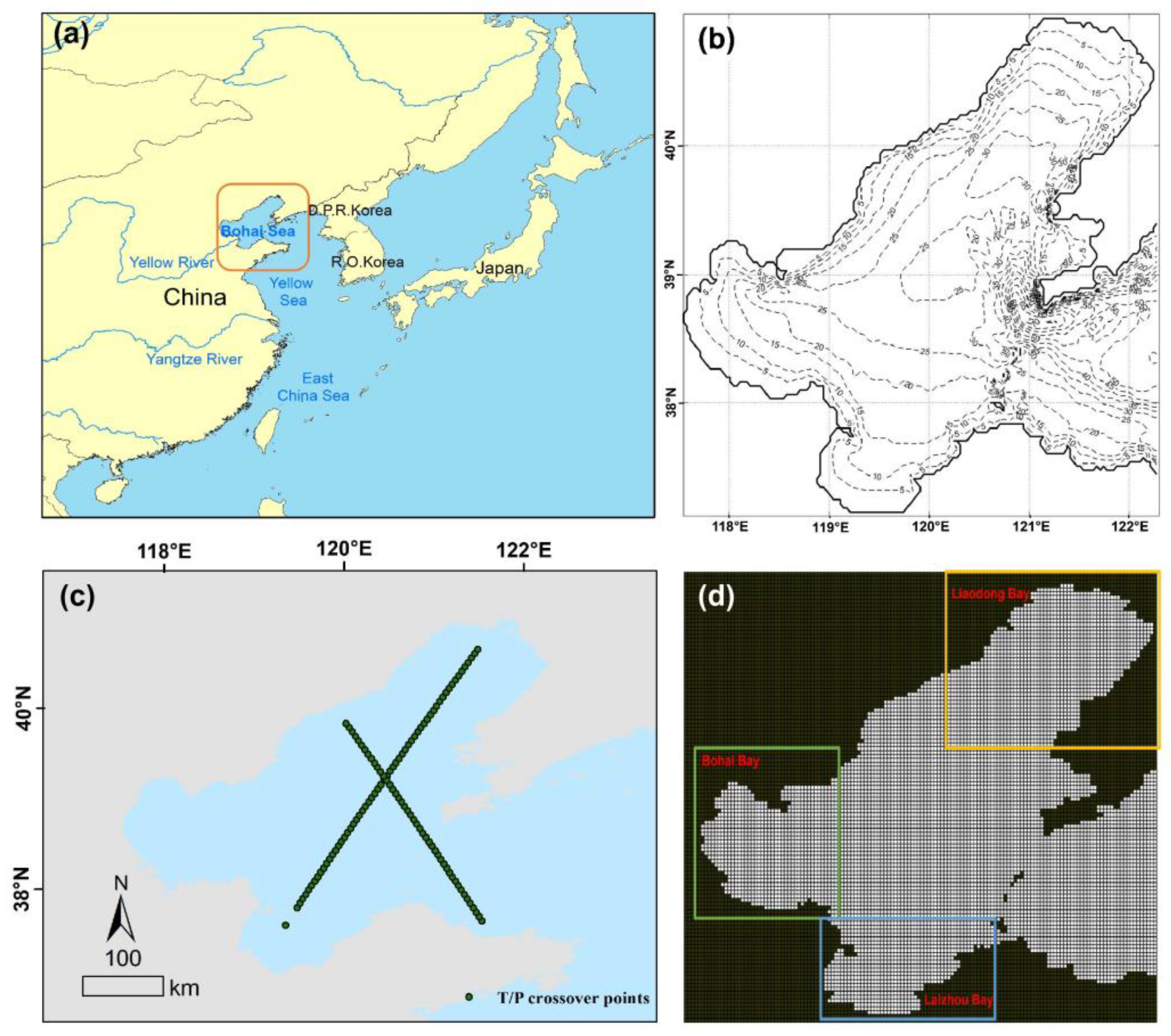
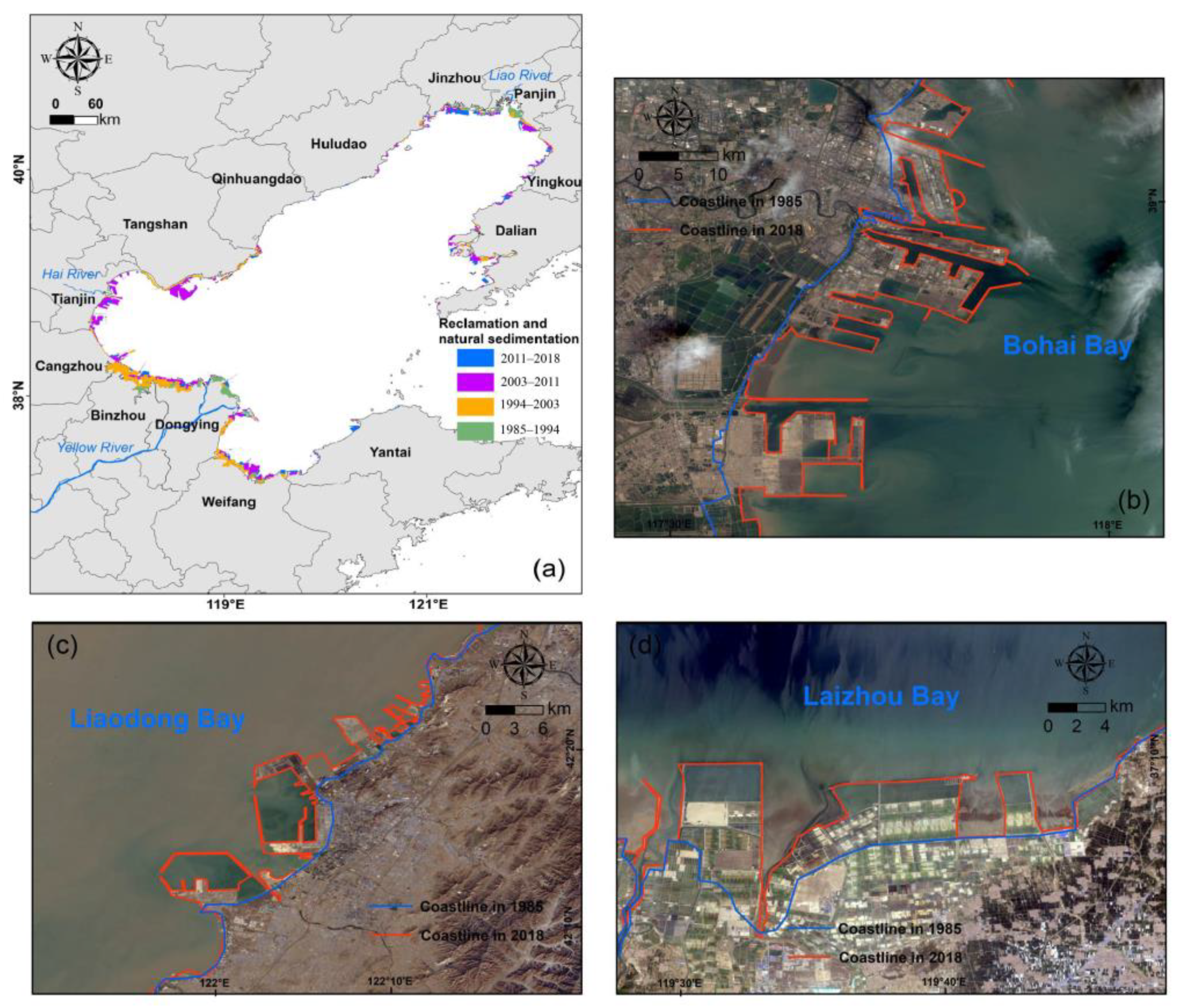
2.1. Study Area

The BHS is a semi-enclosed continental shelf sea in the Northwest Pacific between 37–41°N and 117–122°E (Figure 1). It is connected with the Yellow Sea through the narrow Bohai Strait between Shandong and Liaodong Peninsulas. Its sea area is about 77,000 km2, with a coastline of close to 3800 km, a maximum depth of 70 m, and a mean depth of 18 m [29]. Additionally, the BHS has three bays, including the Liaodong Bay (north of 40°N), Bohai Bay (west of 118°E), and Laizhou Bay (south of 37°N). Most of the BHS has a mixed semidiurnal tide. The tides are predominately semidiurnal, with a maximum range of 4 m and surface tidal currents reaching maximum values of 0.7–2 ms−1 during neap and spring tides, respectively [30]. The M2 tidal constituent is the principal tidal constituent in the BHS. There are two amphidromic points: one close to the coast near Qinhuangdao city and the other off the Yellow River Delta [31].

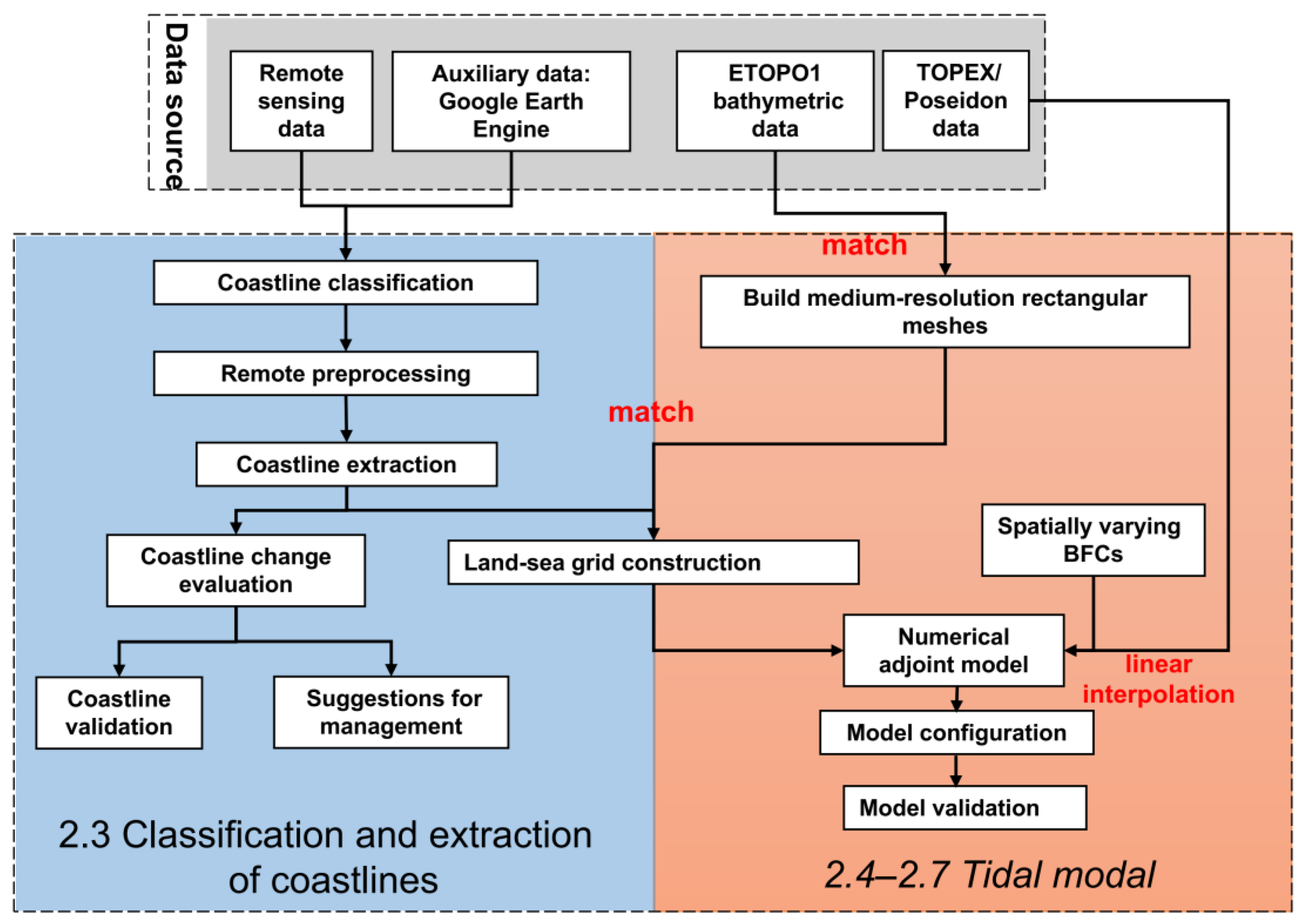
2.2. Data Source and Technological Route

The data used in this study are mainly from the following three groups: The first group was the multispectral remote sensing images from the Landsat satellite, which was launched by the Geospatial Data Cloud (http://www.gscloud.cn (accessed on 20 September 2021)) (Table 1). Based on a time interval of 10 years to represent the temporal changes, the existing data that are cloudless could not always meet the demand of exactly 10 years. Thus, the five scenes at 1985, 1994, 2001, 2009, and 2018, were selected. From the four individual periods of analysis covered by the images (1985–1994, 1994–2001, 2001–2009, and 2009–2018) we constructed a BHS diagram of the spatiotemporal coastline change. The Google Earth Engine is a web-based platform that provides numerous analysis-ready Earth observation datasets at a global scale as a geographic reference for identifying and correcting marine constructions such as ports, wharves, and dams. The second group was the ETOPO1 ocean bathymetry and land topography data, which were downloaded from https://data.nodc.noaa.gov (accessed on 20 September 2021). They are currently among the global land–sea topography data with the highest spatial resolutions. In this study, the land–sea grid (the spatial resolution was 1/60° × 1/60°) rendering using ETOPO1 data was realized. The third group was the primary missions of altimeters, including the tidal harmonic constants derived from 25 years of TOPEX/Poseidon (T/P) observations, which were used for a two-dimensional tidal model in the BHS.
In this study, based on GIS and remote sensing technologies, a coastline interpretation identifier for identifying the coastline in the BHS was proposed, and a two-dimensional tidal model with a data assimilation method was used to simulate the hydrodynamic changes. Herein, the technological framework is shown in Figure 2. The goals were: (1) to establish the coastline interpretation identifier for identifying the extent of the existing coastal reclamation; (2) to reveal the characteristics of the spatiotemporal changes in the coastline and reclamation; and (3) to simulate the responses of the hydrodynamic changes in the coastline.

2.3. Classification and Extraction of Coastlines

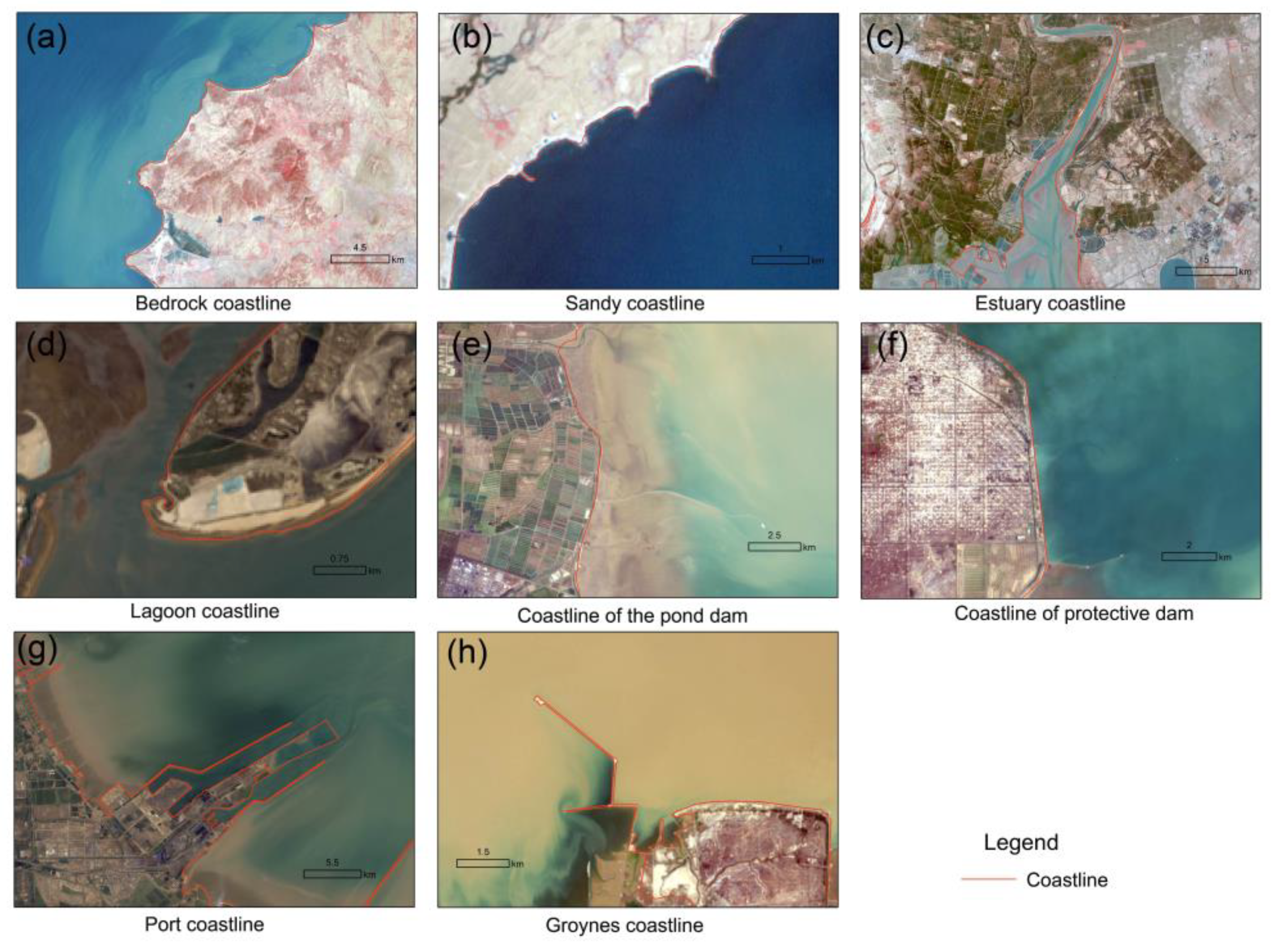
2.3.1. Coastline Classification

Considering the actual situation of the BHS, its coastline was divided into seven categories: estuary coastline, bedrock coastline, sandy coastline, lagoon coastline, pond coastline, protective dam coastline, and marine construction coastline. Human structures included those built in the marine environment for a wide range of purposes, such as foreshore defense (for example, breakwaters and protective dams), transport infrastructure, and commercial developments (for example, bridges and ports) as well as fisheries (aquaculture ponds). Hence, the artificial coastline was divided into protective dam coastline, marine constructions coastline, and pond coastline. The tidal correction was not considered in this study. Although the coastlines we obtained were instantaneous waterlines based on Landsat images, only part of which were natural coastlines whose positions were slightly affected by the tides, this did affect the subsequent analysis and research on the historical evolution of the coastline.

2.3.2. Coastline Extraction

Currently, coastline extraction is mainly realized with automatically detection algorithms or traditional visual interpretation based on the land-sea boundary [32]. However, different interpretation standards are applied for different coast types [33]. Many hard structures (e.g., ports, breakwaters, and groynes) aimed at stabilizing coastlines or protecting infrastructure are specifically designed to create physical barriers to the movement of water and sediments, which are often not incorporated into the numerical models. Therefore, it is necessary to establish a new coastline marking method to study the hydrodynamic changes caused by the coastal changes. The method for identifying the coastline followed these three steps:
The first step was satellite remote sensing image processing, in which the image cutting, radiometric calibration, geometric correction, image mosaic, and band fusion of the land satellite image data were conducted according to ENVI 5.3. Thus, a remote sensing image database of coastal water in the study area in multiple years was established.
The second step was visual interpretation. The regional physical geography, topography, vegetation types, the development and utilization status, field surveys, and auxiliary data (elevation vector data, etc.) were used to establish the relationships of the remote sensing image shape, size, color or tone, shadow, location, structure, texture, and other features with the corresponding interpretation types, and thus to form a unified standard for the description of the characteristics of all types of remote sensing images and to determine their interpretation signs (Figure 3). The original materials were very important to quantify the spatial locations of the offshore architecture (Table 2).
The third step was coastline extraction. With the interpretation signs as references, the human–computer interaction identification method was used to describe the spatial position of the coastline in the near coastal water in ArcGIS 10.1.

2.3.3. Coastline Change Evaluation

To compute the rates of change in coastline position, we used the ArcMap extension module Digital Shoreline Analysis System (DSAS 5.0), which generates a landward baseline from which orthogonal transects are cast at 3 km intervals, and the intercepts between transects and coastlines were recorded [34]. A total of 1414 change rates, each corresponding to a DSAS transect, were thus determined. The end point rate was calculated by dividing the distance of the total coastline movement by the time period between the initial and newest measurements at every transect [35]. In this study, DSAS was employed for analysis of the coastlines by end point rate. This was further analyzed in DSAS with an add-on tool [36] that is downloaded from the USGS website.

2.3.4. Coastline Validation

To verify the method of coastline extraction, a total of 100 control coordinate sites that covered all coastline types were collected from Google Earth images to verify the accuracy of the visual interpretation of the coastline. The overall accuracy was 13.4 m, which was a good performance [37].

2.4. Land–Sea Grid Construction

The grid construction was implemented with the following steps:
Step 1: A two-dimensional (2D) hydrodynamic model with medium-resolution square meshes (the spatial resolution was 1/60° × 1/60°) fitting the coastline was constructed using the Arakawa C grid.
Step 2: The ETOPO1 bathymetric data were matched to the grids, and the values of the rest nodes were interpolated.
Step 3: The coastline in each grid versus the water depth was matched, and the grids were divided based on the dryness and wetness to obtain the control field of the land–sea distribution (Figure 1d).

2.5. Numerical Adjoint Model

Through a numerical adjoint model, the T/P altimeter data could be directly assimilated into the model under the constraints of dynamical equations. In this study, the distributions of the M2 tidal constituent in the BHS in 1985, 1994, 2003, 2011, and 2018 were simulated.
  • Governing equations of forward model
The governing equations for vertically integrated equations of continuity and momentum [35]:
ζ t + 1 a [ ( h + ζ ) u ] λ + 1 a [ ( h + ζ ) v cos ϕ ] ϕ = 0 , u t + u a u λ + v R u ϕ u v tan ϕ R f v + k u u 2 + v 2 h + ζ A Δ u + g a ( ζ ζ ¯ ) λ = 0 , v t + u a v λ + v R v ϕ + u 2 tan ϕ R + f u + k v u 2 + v 2 h + ζ A Δ v + g R ( ζ ζ ¯ ) ϕ = 0 .
where t is the time, λ and ϕ are the east longitude and north latitude respectively, ζ is the sea surface elevation above the undisturbed sea level, u and v are the east and north components of fluid velocity respectively, ζ ¯ is the adjusted height of equilibrium tides, R is the radius of the earth, a = R cos ϕ , f = 2 Ω sin ϕ , where Ω represents the angular speed of earth’s rotation, g is the acceleration due to gravity, h is the undisturbed water depth and h + ζ denotes the total water depth, k is the BFC, A is the coefficient of horizontal eddy viscosity, Δ is the Laplace operator and Δ ( u , v ) = a 1 [ a 1 λ ( λ ( u , v ) ) + R 1 ϕ ( cos ϕ ϕ ( u , v ) ) ] .
  • Adjoint equations
The cost functions, which are measured as the differences between observations and simulation results, were minimized by optimizing the control variables. The numerical schemes for the cost function and the Lagrangian function in this section are based on Lv and Zhang [37]. The cost function is defined as:
J ( ζ ) = 1 2 K ζ ( ζ ζ ^ ) 2 d σ ,
and the Lagrangian function is defined as:
L = [ μ ( u t + u a u λ + v R u ϕ u v tan ϕ R f v + k u u 2 + v 2 h + ζ A Δ u + g a ( ζ ζ ¯ ) λ ) + ν ( v t + u a v λ + v R v ϕ + u 2 tan ϕ R + f u + k v u 2 + v 2 h + ζ A Δ v + g R ( ζ ζ ¯ ) ϕ ) + τ ( ζ t + 1 a [ ( h + ζ ) u ] λ + 1 a [ ( h + ζ ) v cos ϕ ] ϕ ) + 1 2 W ( ξ ξ ^ ) 2 ] d S + J ( ζ ) ,
  • Correction equations
The correction relation of the Fourier coefficients on an open boundary is:
K b ( a i , l a i , l ) + j = 1 J T l j cos ( ω i j Δ t ) = 0 , i = 0 , , M 0
K b ( b i , l b i , l ) + j = 1 J T l j sin ( ω i j Δ t ) = 0 , i = 1 , , M 0
where { ω i : i = 1 , , M 0 } is the angular frequency of the considered tide and { a i , l , b i , l : i = 1 , , M 0 } are the Fourier coefficients derived from assimilation.

2.6. Estimation Algorithm of Spatially Varying BFCs

The satellite observations from TOPEX/Poseidon were assimilated during the BFC optimization in this study with an enhancement in the spatial resolution of the numerical model. In the estimation of BFCs, some grid points were appointed as independent coefficients, and the values of BFCs in the entire area could be obtained through linear interpolation using these independent coefficients. Assuming b m , n is a series of independent BFCs and k j , k are the result of linear interpolation with b m , n , we adopted the following relation [38]:
k j , k = m , n ϕ j , k , m , n b m , n ,
where ϕ j , k , m , n is the coefficient of linear interpolation ( ϕ j , k , m , n = W j , k , m , n / m , n W j , k , m , n ), W j , k , m , n is the weighted coefficient ( W j , k , m , n = ( R 2 r j , k , m , n 2 ) / ( R 2 + r j , k , m , n 2 ) ) of the Cressman form, r j , k , m , n is the distance from grid point ( j , k ) to ( m , n ) , and R is the influence radius, taken as 2 here.
The gradients of the Lagrangian function with respect to an independent BFC are as follows:
L b m , n = i , j , k ( ϕ j , k , m , n + ϕ j + 1 , k , m , n 2 × u a j , k i + 1 r j , k i ( α u j , k i + 1 + ( 1 α ) u j , k i ) h j + 1 / 2 , k + ξ j + 1 / 2 , k i ) + i , j , k ( ϕ j , k , m , n + ϕ j , k + 1 , m , n 2 × v a j , k i + 1 s j , k i ( α v j , k i + 1 + ( 1 α ) v j , k i ) h j + 1 / 2 , k + ξ j + 1 / 2 , k i ) ,
where i is the index of time. Because the cost function decreases along the opposite direction of the gradient, we can obtain the correction of the independent BFC as:
K c ( b m , n b m , n ) + L b m , n / L b 2 = 0 ,
i.e.,
b m , n = b m , n 1 K c L b m , n / L b 2 = 0 ,
where:
L b 2 = ( m , n L b m , n 2 ) 1 / 2 ,
where b m , n and b m , n are the prior and optimized values of an independent BFC, respectively, and K c is a constant. In our model, the L / b m , n , i.e., the gradient of the Lagrangian function with respect to the independent BFC, was unitized first, which means that only the direction of the gradient was used when the optimization was performed. A small positive value was assigned to 1 / K c in order to ensure that the cost function could decrease continuously without fluctuations. In our model, the initial value was set to 0.002, and 1 / K c was taken as 10 4 , i.e., K c = 10 4 , which was obtained through a trial-and-error procedure.

2.7. Model Configuration

The computing area was the Bohai Sea, covering from 37°N–41°N and 117.5°E–122.3°E. The spatial resolution in this model was 1/60° × 1/60°, and the gridded topography was based on the ETOPO1 data, while the deepest water depth of the computing area was 85 m. Additionally, the model adopted the Arakawa C grid, where the water level was defined at the center, and the two velocity components were defined to be perpendicular to the edges of the cell.
The closed boundary conditions for our model were zero flow normal to the coast. That is, u · n = 0 for the grid points at the closed boundary, where n is the outward unit vector and u = ( u , v ) is the velocity vector. In the present study, Beijing standard time (referring to the meridian of 120°E) was adopted throughout.
Along the open boundaries, the water elevation of the M2 tide at the j t h time step was given as ζ m l , n l j = a 0 , l + [ a l cos ( ω j Δ t ) + b l sin ( ω j Δ t ) ] , where ( m l , n l ) stands for the grid points at the open boundaries, ω is the frequency of the M2 constituent, and a l and b l are the Fourier coefficients. The open boundary conditions of water elevation were obtained by assimilating the T/P data using the adjoint method and were fixed in all experiments [31].

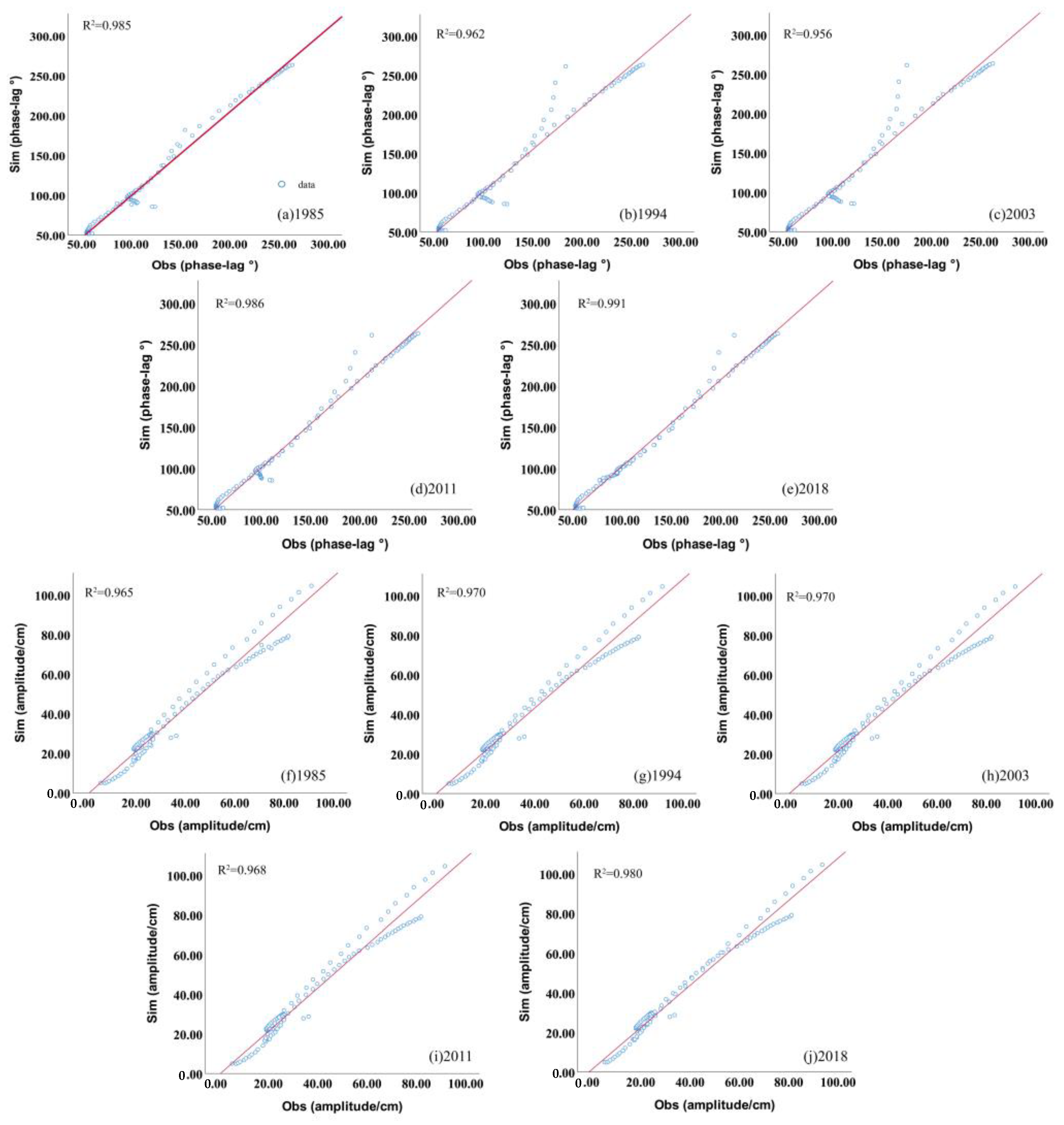
2.8. Model Validation

The harmonic constants at 108 T/P satellite altimeter crossover points, as shown in Figure 1c, were used as observations to verify the model’s fidelity and the evaluation criteria, including the amplitude difference, phase-lag difference, and vector difference [28]. The model’s performance was evaluated by the root-mean-square errors (RMSE) and mean absolute errors (MAE), which are widely used to represent the discrepancy between the simulated and observed harmonic constants [37]. As listed in Table 3, The deviations between the simulated results and observations are listed in M2. The MAE in the amplitude and phase between the simulation and measurements were smaller than 3.1 cm and 5.4°, respectively, and the vector difference was smaller than 5.1, implying a successful simulation [26]. The RMSEs between the simulated results and measurements were also calculated. The averaged absolute differences in amplitude were only 2.9 cm, 2.8 cm, 2.8 cm, 2.8 cm, and 3.1 cm for the 1985, 1994, 2003, 2011, and 2018 tides, respectively. The averaged absolute differences in phase lag were 8.1°, 7.2°, 7.7°, 5.8°, and 5.7° for the five tides, respectively. The MAEs and RMSEs of the five parameters met the requirements [37]. Additionally, for the R2 results for five years, the simulated results had a significant correlation with the measurements (Figure 4).

3. Results

3.1. The Changing BHS Coast

3.1.1. Reclamation and Sedimentation

Figure 5a shows the spatial distribution of reclamation and sedimentation from 1985 to 2018, which were mainly concentrated in the Bohai Bay (36.5%), Laizhou Bay, (20.6%) and the southern side of the Liaodong Bay (18.0%). A huge amount of sediment from the loess region has formed a megadelta in the Yellow River Estuary with an area of 250.4 km2. Additionally, this phenomenon also occurred in the Liao River and Hai River Estuary. Artificial reclamation was widely distributed along the whole coastline of the BHS; coastal projects such as ports, ponds, and bridges bulged along the coast; and large-scale industrial areas from reclamation settled down and were scattered in the coastal water of the BHS (Figure 5b–d).

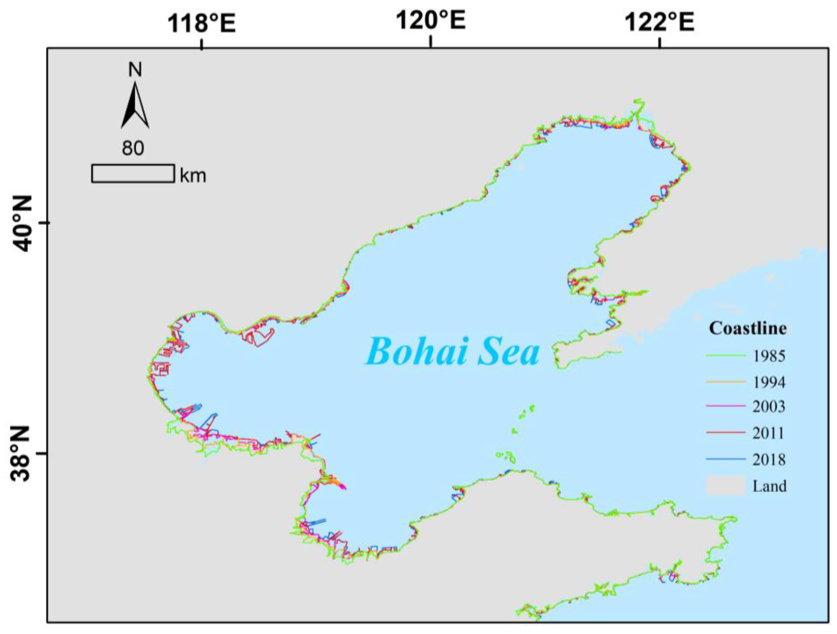
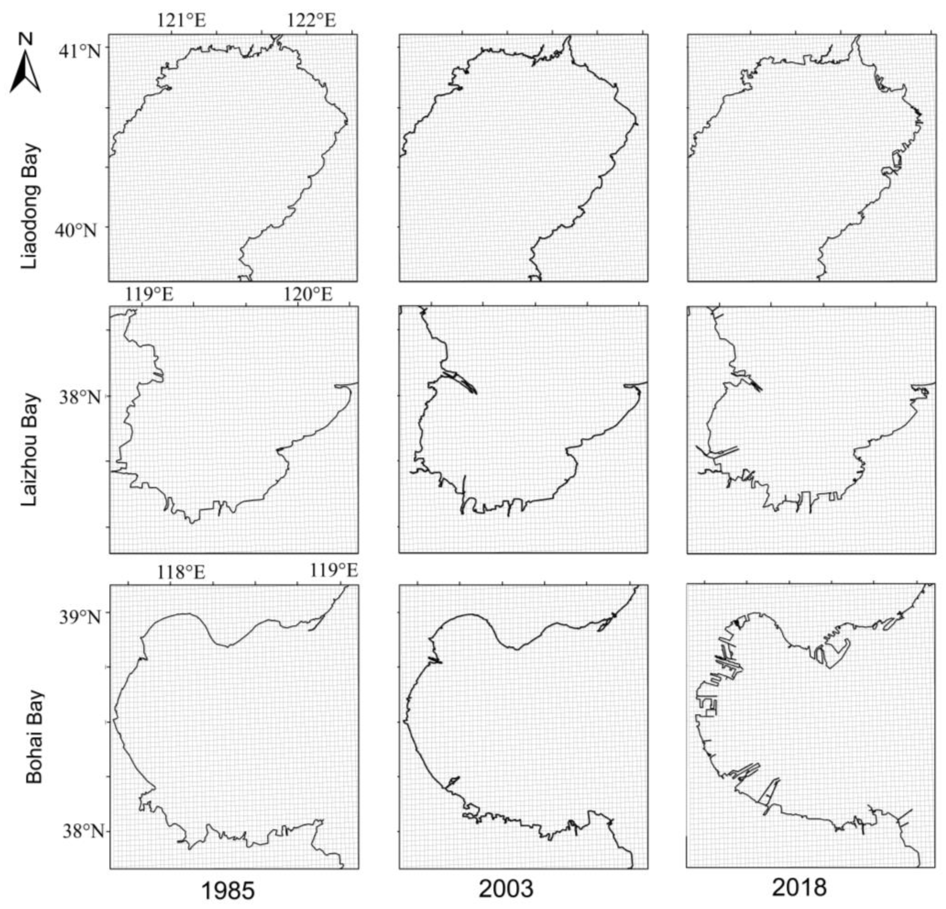
3.1.2. Change in Coastline

In the past 34 years, the BHS has already shown significant spatiotemporal changes in its coastline (Figure 6). Our findings reveal that reclamation projects such as ports and wharves are bulging along the coast, moving the coastline seaward at an average accretion rate of 29.3 m/yr and a maximum accretion rate of 492 m/yr, which occurred near the coast of Tianjin City. The coastline change at long time scales was dominated by reclamation. Around 72.9% of the coastline of the BHS mapped in 2018 had seaward movement occur compared to its position in 1985. This phenomenon was mainly distributed in the Laizhou Bay, Liaodong Bay, and Bohai Bay (Figure 7).

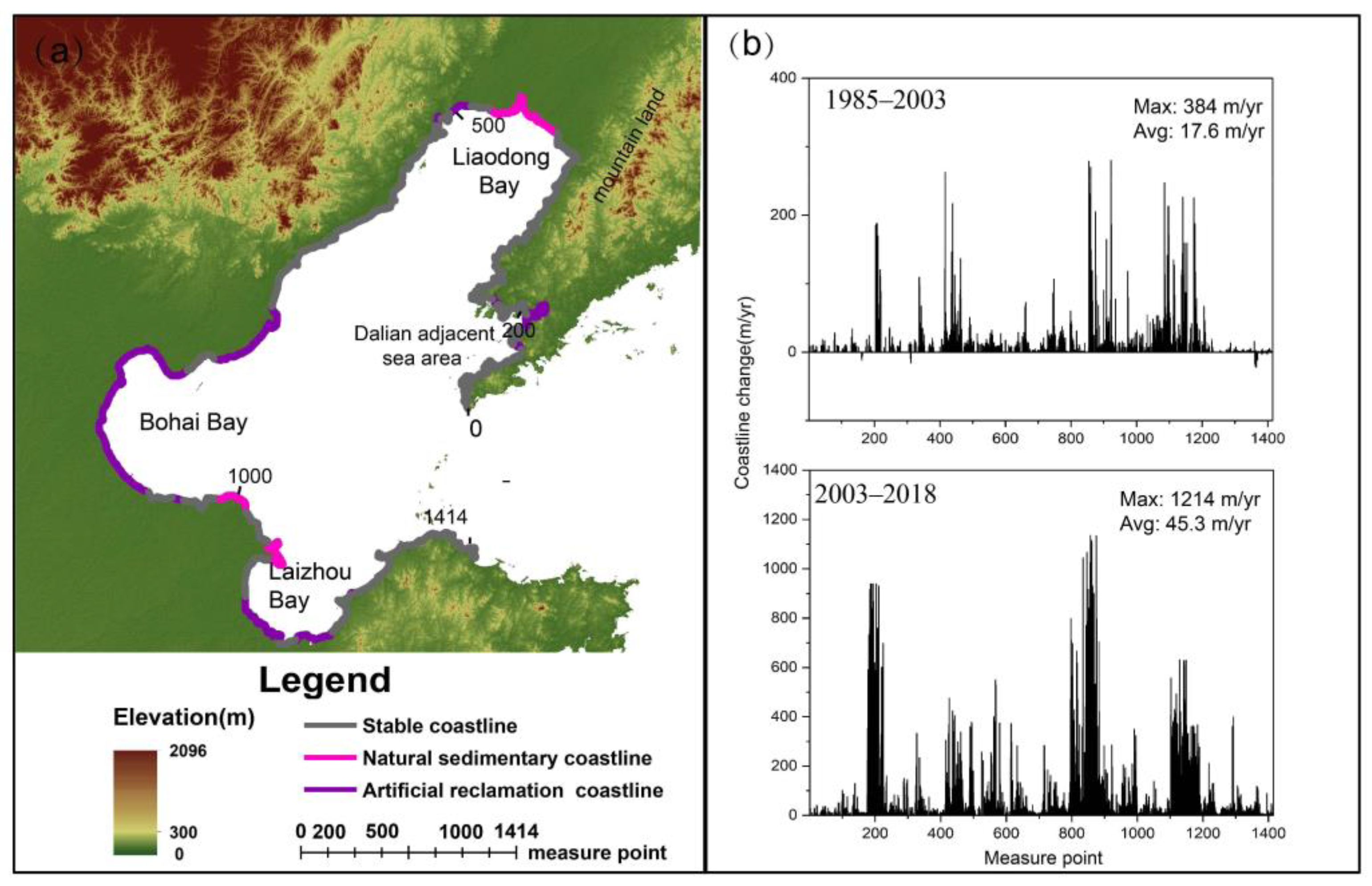
3.1.3. Analysis of Coastline Movement

Between 1985 and 2018, the average net coastline movement reached 996 m (29.3 m/yr), and the maximum reclamation distance into the sea was 492 m/yr. In terms of different periods, the net result of the coastline changes between 1985 and 2003 was artificial reclamation and natural sediment deposition. The mean net coastline movement of the former was 359 m, that of the latter was 260 m, and the mean of both was 318 m (17.6 m/yr). The maximum annual average reclamation distance to the sea was 384 m/yr, which was located in the coastal waters of Dalian City (Figure 8a). Between 2003 and 2018, the mean net coastline movement of artificial reclamation was 2003 m, that of natural sedimentation was 184 m, the mean of both was 815 m (45.3 m/yr), and the maximum reclamation distance into the sea was 1214 m/yr, which was located in the new Tianjin coastal area.
The results revealed that around 66.3% of the coastline of BHS mapped in 2003 was within 99~129 m of its position in 1985, which was mainly distributed in the northwest, northeast, and southeast of BHS. However, only 31.3% of the coastline of BHS mapped in 2018 was within 0~140.4 m of its position in 1985, and more than 30% of the coastline expanded more than 1 km to the sea (Figure 8b). Furthermore, there has been a significantly decrease in the proportion of stable boundary (currently 27.1% compared to 57.5% prior to 1985). In contrast, the annual average net coastline movement since artificial reclamation commenced was about 2.1 times faster than the rate prior to 2003.

3.2. Responses of Hydrodynamics to Changes in Coastline

3.2.1. Sea Surface Area, Kinetic Energy, and Sea Water Volume

As shown in Table 4, the sea surface area and sea water volume of the BHS in 1985, 1994, 2003, 2011, and 2018 both show decreasing trends, while the kinetic energy shows a fluctuating upward trend within the five periods. From 1985 to 2018, the volume decreased by 0.17%, the surface area decreased by 4.54%, and the kinetic energy increased by 2.53%. Among them, the three parameters show the largest difference changes during 2003–2011. Meanwhile, the seaward expansion of artificial reclamation and natural sedimentation reached a peak value (2639.5 km2), especially the expansion of marine buildings such as ports and wharves, which contributed to the obvious spatial changes in the coastline (Figure 6).

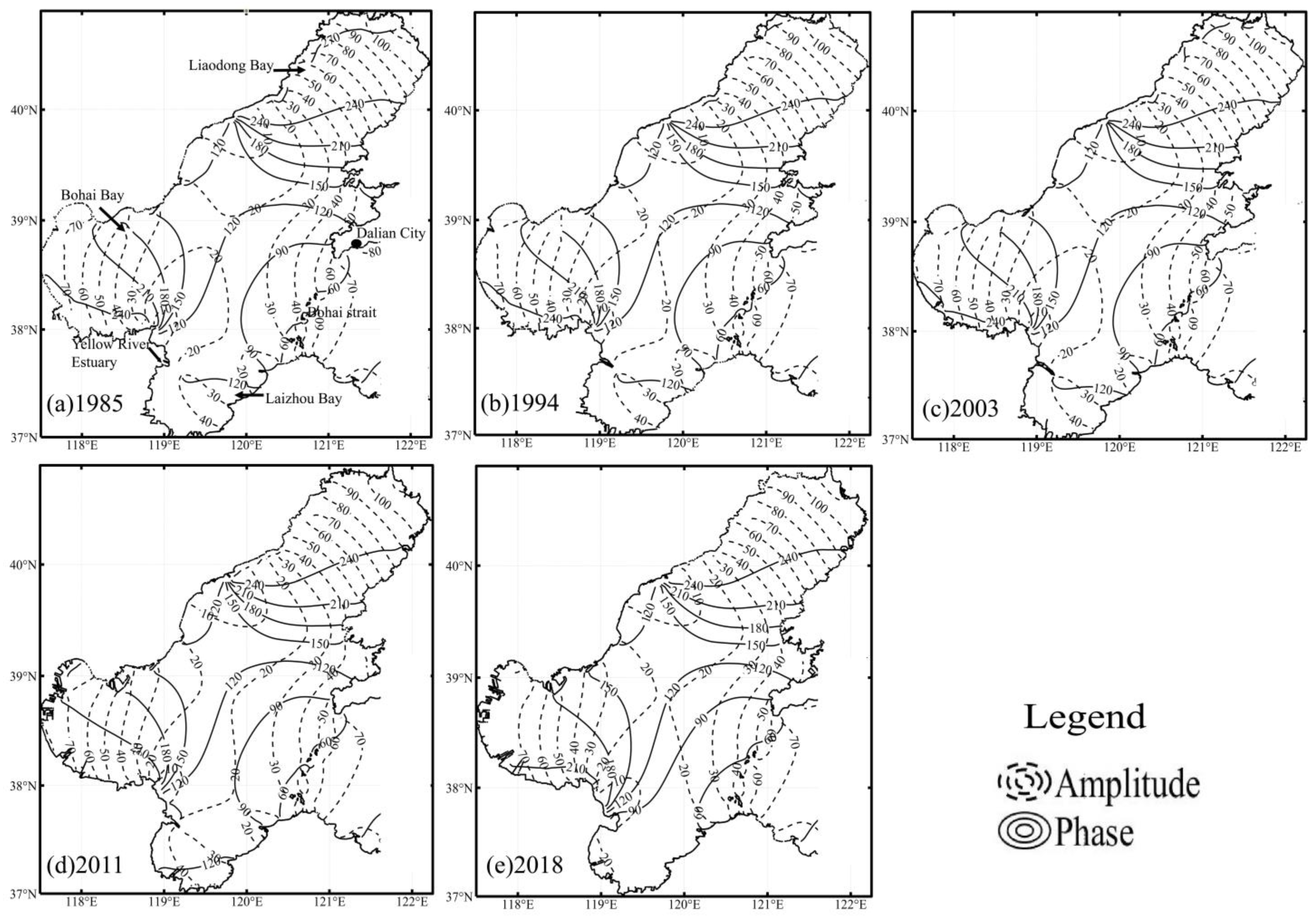
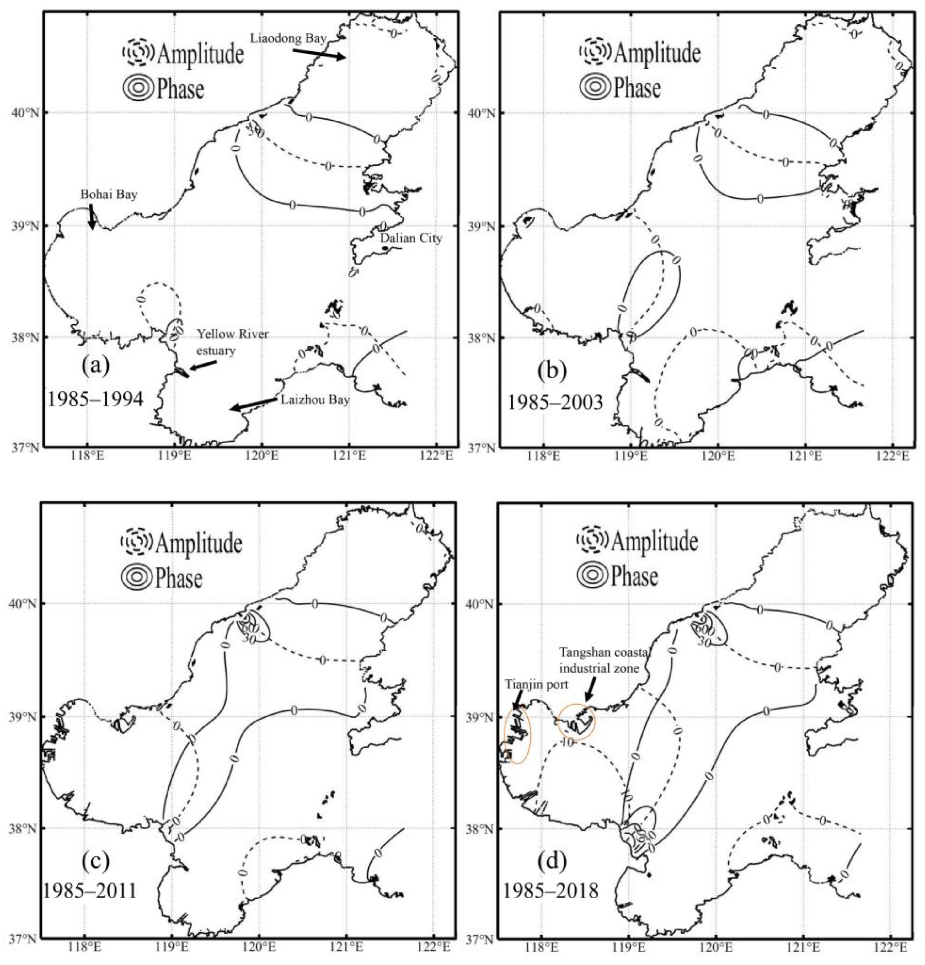
3.2.2. Effect on the M2 Tidal Constituent

The cotidal charts in 1985, 1994, 2003, 2011, and 2018 are shown in Figure 9. From Figure 9, we can see that the M2 tidal constituent propagated mainly from the Bohai strait into the BHS, and then a main branch of it propagated northeastwards into the Liaodong Bay though the area adjacent to the southeast of Qinhuangdao City, while the other branch propagated westwards into the Bohai Bay though the Yellow River Estuary. The smallest amplitude of the M2 tidal constituent (lesser than 80 m) appeared at the central Bohai Straits. In the five periods of the simulation, the amplitude of the M2 tidal constituent in the BHS had obvious temporal and spatial variations, but the difference in the phase lag of the M2 tidal constituent was not significant.
Figure 10 shows the differences in the amplitude and phase lag of the M2 tidal constituent in the BHS under four work conditions during 1985–1994, 1985–2003, 1985–2011, and 1985–2018. Due to the change in the coastline, the amplitudes of the M2 tidal constituent retained their increases in the four cases. In the 1985–2011 simulation, the coastline changes in the Bohai Bay caused by artificial reclamation (e.g., the Tianjin port and the Tangshan coastal industrial zone) were the major factors that remarkably altered the M2 tide amplitude. Compared with the 1985 case, the amplitude increase of the M2 tidal constituent in the Bohai Bay was 6–14 cm in 2018, and the deviation in the position of the amphidromic point was significant, which led to the drastic change in the phase lag on the northern coast of the Yellow River Estuary and the adjacent sea area of Dalian.

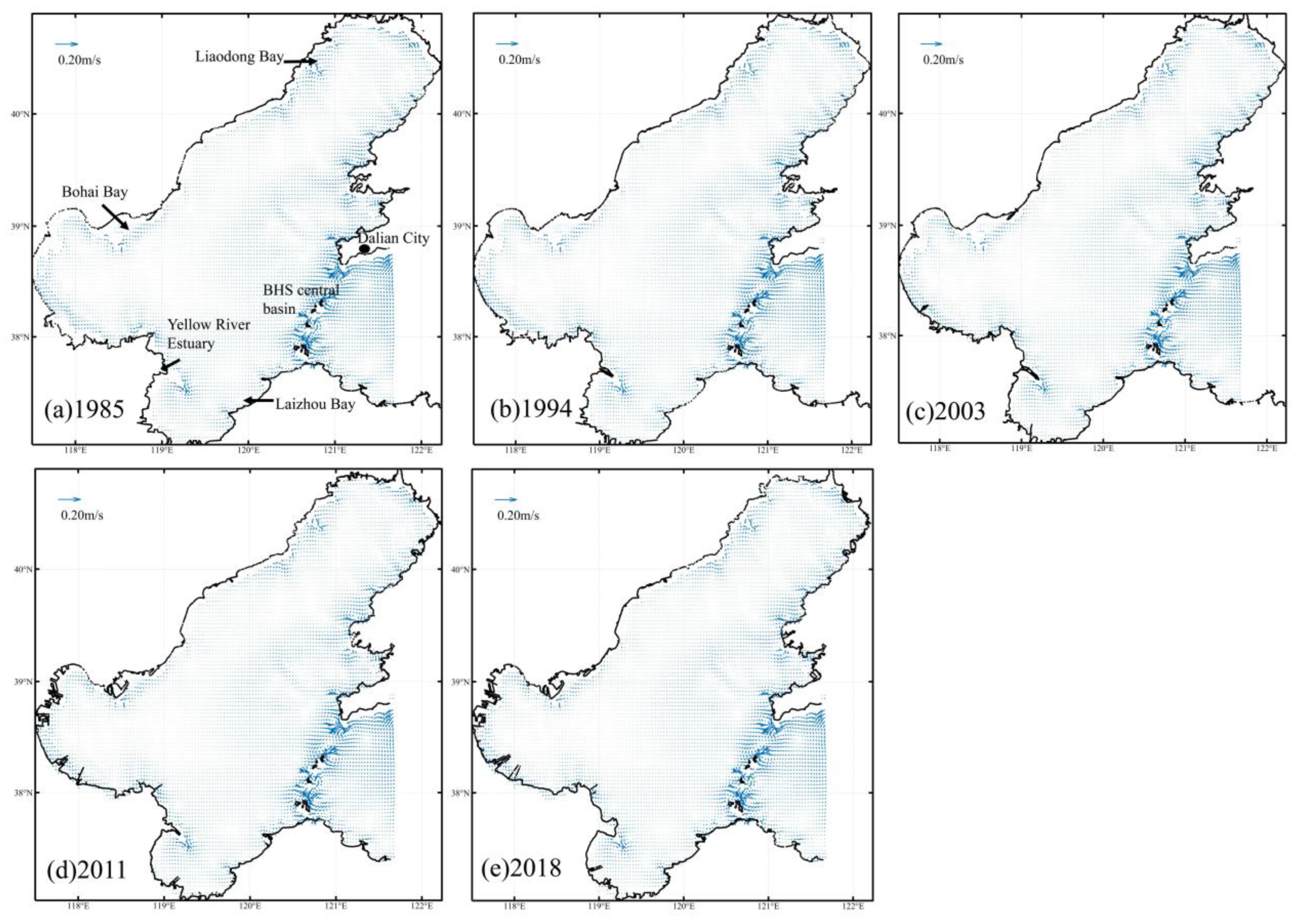
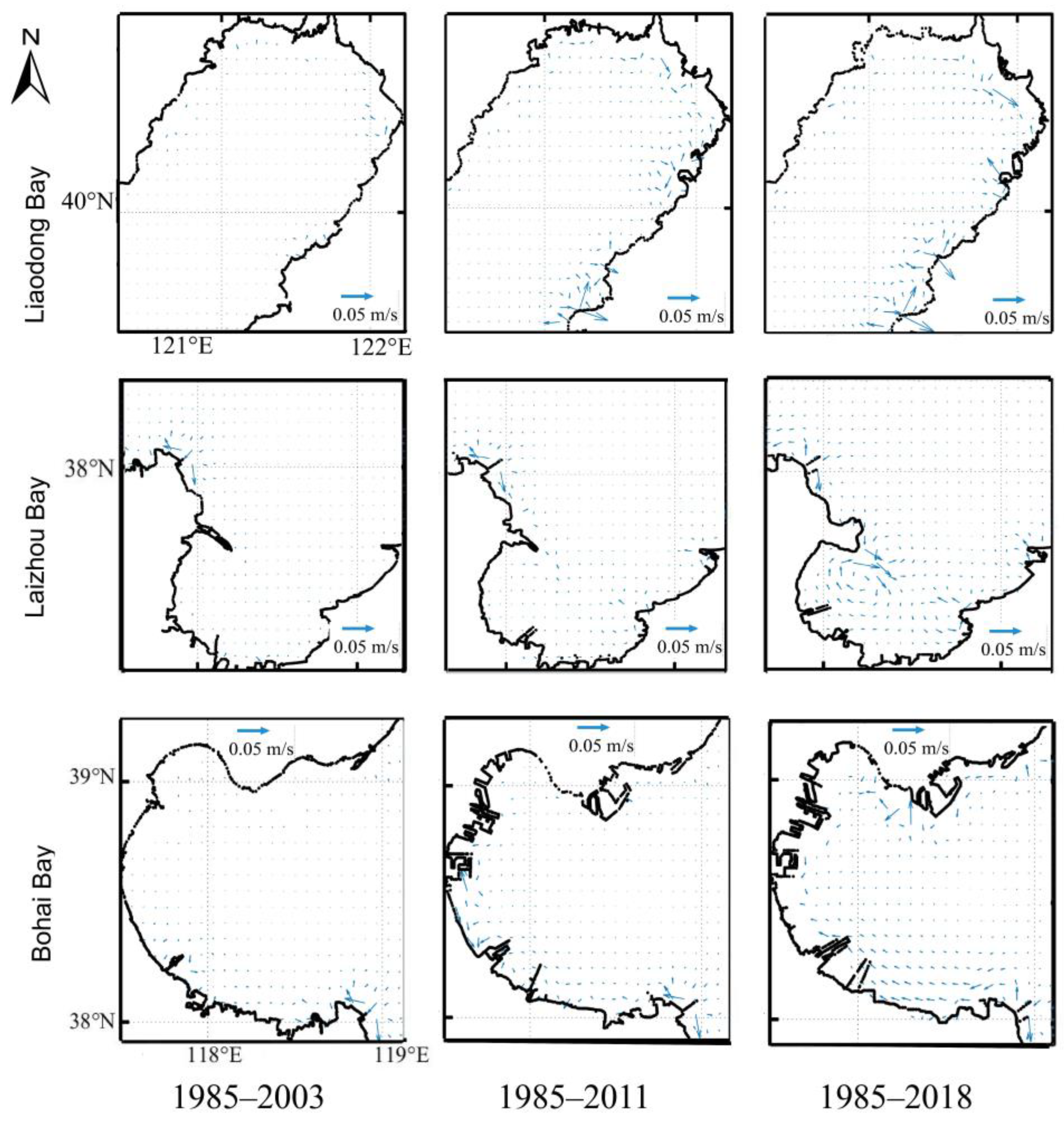
3.2.3. Effect on Residual Current (RC)

From Figure 11, the RC’s changes in spatiotemporal characteristics were not significant in the cases of 1994, 2003, 2011, and 2018. RC (>0.05 m/s) was mainly concentrated in the central basin of the BHS and the adjacent sea area of Dalian.
In order to identify the residual current change effected by coastline changes, the simulation results of 1994, 2003, 2011, and 2018 were subtracted from 1985. The RCs displayed an overall increasing trend from 1985 to 2018 in the Bohai Bay, Laizhou Bay, and Liaodong Bay (Figure 12). Due to the construction of reclamation projects, the residual flow velocities in the waters near the Yellow River Estuary and the eastern coast of Liaodong Bay increased considerably, with a maximum increase of 0.11 m/s. The increases in the residual flow velocities in the waters near the Laizhou Bay and Bohai Bay were generally between 0.01 and 0.03 m/s.

4. Discussion

4.1. Evaluation of Coastline Change

This study presents a systematic analysis of coastline change movements along the BHS coastal area during the period of 1985–2018. According to our statistics, only 16.1% of the coastline exhibited statistically significant sedimentation, which occurred in major estuaries. The high-intensity human activities, such as reclaiming land from the sea, continue to disturb the coastline and caused the proportion of coastline change to increase sharply from 42.5% in 1985 to 72.7% in 2018. We compared the results over the same period and found that the overall error was 5.0–12.1% [33,39] (pp. 101–105). Factors affecting the coastline’s changes included reclamation and coastal sedimentation. Based on the result for the area, reclamation was the dominant factor leading to the change in the coastline, and its contribution rate reached 94.2% (Figure 8a). We compared the results over the same period and found that the overall error was 5.3–5.7% [22].
Studies showed that high-intensity coastal reclamation is mainly driven by the booming economy and growing population [40]. Since 2000, a number of national coastal economic zones, including the Tianjin Binhai New Area, the Liaoning Coastal Economic Zone, and the Shandong Peninsula Blue Economic Zone, have been implemented, and the population density in coastal areas has increased, leading to land shortages on the coast of the BHS [18]. In order to have more land for residence and commercial development, a series of reclamation activities have been launched in the coastal area of the BHS, and the natural coastline was used for ports, followed by the aquaculture pond, while some sea areas are also used for the salt industry. Meanwhile, many ports have been built up in this area to meet the need for the large trade throughput. Affected by industrial and port construction, from 1985 to 2018 the rate of coastline change in the Bohai Bay was the fastest in the BHS. A total of 1826 km2 was reclaimed from the sea, which resulted in the entire coastline moving seaward by 6.8 km.

4.2. Evaluation of Hydrodynamics Change

The numerical simulation results showed that the reclamation projects led to a slight increase in tide RCs and enhanced the amplitude of the M2 tidal constituent. Additionally, a part of the tidal energy was dissipated by the reclamation projects, which resulted in an increase in kinetic energy. The assessment results of the tidal model in the BHS were compared with the spatial distribution of the amplitudes of the M2 tidal constituent published by Zhu et al. [27] over the same period. According to the comparison of the spatial distribution, the amplitudes of the M2 tidal constituent changed up to 10 cm in the Bohai Bay. Their simulated results in the BHS between 1987 and 2016 were similar to the present ones. However, their response for RCs was generally larger in the western coast of the Bohai Bay. This discrepancy may have been caused by an insufficient optimization of the BFCs. To our knowledge, studies on the effects of coastline change on its tidal dynamics in the BHS remain insufficient, mainly in space-varying BFCs. Zavala-Garay et al. [41] investigated the effects of bottom topography on the tides. They found that the tidal current velocity was mainly driven by residual currents produced by space-varying bottom friction. Qian et al. [26] further estimated the spatially varying BFCs in the BHS. They found that bottom friction plays an important role in the performance of numerical models in the BHS. Therefore, regional-scale Earth observation studies that compare tidal dynamics without the effects of bottom topography may be inadvertently exposed to these spatial and temporal tidal biases, potentially resulting in misleading estimates of tidal changes [42]. In this study, by combining remote sensing technology and hydrodynamic simulation technology, we were able to build a land–sea grid (the spatial resolution was 1/60° × 1/60°) where the coastline migrating process adequately adapted to tide effects. Figure 9, Figure 10, Figure 11 and Figure 12 demonstrate the effectiveness of this technique, with extensively affected tide coastlines within the coastal water of the BHS.

4.3. Suggestions for Management of Coastal Reclamation

Long-term coastline change indicates that the embayment of the BHS is undergoing reclamation. The rapid expansion of the coastal economy and accelerated coastal population growth has caused a sharp increase in land reclamation, especially on the western coast of the Bohai Bay and the north coast of the Laizhou Bay, with silty, sandy shoals and low-level terrain. In order to obtain more space for further development in agriculture and industry, intensive reclamation projects have taken place there (Figure 6). We suggest that the establishment of a sea area dynamic monitoring system, the implementation of the most stringent management and control measures for sea reclamation, should be carried out to gradually restore and improve the sea water dynamic conditions [43,44]. In addition, our results show that >50% of the natural coastlines have been replaced by seawalls, breakwaters and other hard structures, and large-scale natural waters have been developed into aquaculture and salt fields, impacting the movement of water and sediments. We suggest focusing on economizing sea utilization and scientifically planning the pattern of reclamation projects and the use of marine space. A well-conceived reclamation scheme is very important for the sustainable development of the coastal system [45,46].

5. Conclusions

In this paper, we revealed the spatiotemporal evolution of the coastlines in the Bohai Sea based on a 5-year record of remote sensing images in the last 40 years. From 1985 to 2018, due to the construction of ports and ponds, the BHS coastline has undergone considerable changes. Approximately 40–45% of the water area of the shore has been affected by reclamation projects, most recently in the Tianjin area. The main result of this study is that nearly 30 m/yr is being built out into the bay near the Tianjin City and that this trend is having an effect on the M2 tidal rate by between 6 and 14 cm/yr in the Bohai Bay. The detailed findings of our study are:
  • The coastline showed an overall advancing trend over the 34-year period from 1985 to 2018, which was particularly obvious on the south coast of Laizhou Bay and Bohai Bay. According to the statistics, the average net coastline movement was 996 m (29.3 m/yr), and the maximum reclamation distance into the sea was 492 m/yr. Around 72.9% of the coastline of the BHS mapped in 2018 moved compared with its position in 1985, and more than 30% of the coastline expanded more than 1 km into the sea.
  • During the simulation, reclamation projects have had a great influence on the tidal velocity and direction across the coastline extension. However, the influence is limited, and the inner bay area receives a greater impact, especially in Bohai Bay and Liaodong Bay. The model results show that the change in the coastline increased the amplitude of the M2 tidal constituent in the Bohai Bay by 6–14 cm and increased the RC on the eastern coast of the Liaodong Bay by up to 0.07 (0.01) m/s.

Author Contributions

J.L., conceptualization, data curation, formal analysis, investigation, methodology, software, visualization, writing—original draft, and writing—review and editing; Y.Z., data curation, formal analysis, methodology, supervision, and visualization; X.L., formal analysis, methodology, writing—review and editing, project administration, and resources; H.S., conceptualization, funding acquisition, investigation, validation, methodology, project administration, and resources. All authors have read and agreed to the published version of the manuscript.

Funding

This paper was supported by the National Natural Science Foundation of China (U1806214 and 42076011) and the National Key Research and Development Program (2019YFC1408405).

Data Availability Statement

The satellite altimeter data used in our study can be downloaded from the Radar Altimeter Database System (http://rads.tudelft.nl/rads/rads.shtml, last access: 1 May 2021).

Acknowledgments

The authors were provided valuable suggestions on the identification and extraction methods of the coastline. Wang Yuzhe, Guo Junting, and Cao Ruichen participated in the discussion on the study method and manuscript preparation and provided useful suggestions.

Conflicts of Interest

The authors declare no conflict of interest.

References

  1. Pucino, N.; Kennedy, D.M.; Young, M.; Ierodiaconou, D. Assessing the accuracy of Sentinel-2 instantaneous subpixel shorelines using synchronous UAV ground truth surveys. Remote Sens. Environ. 2022, 282, 113293. [Google Scholar] [CrossRef]
  2. Konlechner, T.M.; Kennedy, D.M.; O’Grady, J.J.; Leach, C.; Ierodiaconou, D. Mapping spatial variability in shoreline change hotspots from satellite data; a case study in southeast Australia. Estuar. Coast. Shelf Sci. 2020, 246, 107018. [Google Scholar] [CrossRef]
  3. Anthony, E.J.; Kestenare, E.; Reyns, J.; Jouanno, J.; Anthony, E.J.; Laibi, R.; Hemer, M.; Penhoat, Y.D.; Ranasinghe, R. Response of the Bight of Benin (Gulf of Guinea, West Africa) coastline to anthropogenic and natural forcing, Part 2: Sources and patterns of sediment supply, sediment cells, and recent shoreline change. Cont. Shelf Res. 2019, 173, 93–103. [Google Scholar] [CrossRef]
  4. Arkema, K.K.; Guannel, G.; Verutes, S.; Wood, A.; Silver, J.M. Coastal habitats shield people and property from sea-level rise and storms. Nat. Clim. Chang. 2013, 3, 913–918. [Google Scholar] [CrossRef]
  5. Paz-Delgado, M.V.; Payo, A.; Gómez-Pazo, A.; Beck, A.-L.; Savastano, S. Shoreline Change from Optical and Sar Satellite Imagery at Macro-Tidal Estuarine, Cliffed Open-Coast and Gravel Pocket-Beach Environments. J. Mar. Sci. Eng. 2022, 10, 561. [Google Scholar] [CrossRef]
  6. Bugnot, A.B.; Mayer-Pinto, M.; Airoldi, L.; Heery, E.C.; Johnston, E.L.; Critchley, L.P.; Strain, E.M.A.; Morris, R.L.; Loke, L.H.L.; Bishop, M.J.; et al. Current and projected global extent of marine built structures. Nat. Sustain. 2020, 4, 33–41. [Google Scholar] [CrossRef]
  7. Pianca, C.; Holman, R.; Siegle, E. Shoreline variability from days to decades: Results of long-term video imaging. J. Geophys. Res. Ocean. 2015, 120, 2159–2178. [Google Scholar] [CrossRef]
  8. Li, P.; Li, G.; Qiao, L.; Chen, X.; Shi, J.; Gao, F.; Wang, N.; Yue, S. Modeling the tidal dynamic changes induced by the bridge in Jiaozhou Bay, Qingdao, China. Cont. Shelf Res. 2014, 84, 43–53. [Google Scholar] [CrossRef]
  9. Lin, S.; Liu, G.; Niu, J.; Wei, X.; Cai, S. Responses of hydrodynamics to changes in shoreline and bathymetry in the Pearl River Estuary, China. Cont. Shelf Res. 2021, 229, 104556. [Google Scholar] [CrossRef]
  10. Zhang, P.C.; Sun, L.Y.; Zhu, Y.L. Reclamation-induced influence on hydrodynamics and suspended sediment concentration at three estuary areas in Bohai Bay. China Harb. Eng. 2015, 35, 6–12. [Google Scholar]
  11. Wang, X.Z.; Zhang, H.G.; Fu, B.; Shi, A. Analysis on the coastline change and erosion-accretion evolution of the Pearl River Estuary, China, based on remote sensing images and nautical charts. J. Appl. Remote Sens. 2013, 7, 073519. [Google Scholar] [CrossRef]
  12. Lin, L.; Liu, Z.; Xie, L.; Gao, H.; Cai, Z.; Chen, Z.; Zhao, J. Dynamics governing the response of tidal current along the mouth of Jiaozhou Bay to land reclamation. J. Geophys. Res.-Ocean. 2015, 120, 2958–2972. [Google Scholar] [CrossRef]
  13. Chu, N.; Yao, P.; Ou, S.; Wang, H.; Yang, H.; Yang, Q. Response of tidal dynamics to successive land reclamation in the Lingding Bay over the last century. Coast. Eng. 2022, 173, 104095. [Google Scholar] [CrossRef]
  14. Byun, D.S.; Wang, X.H.; Holloway, P.E. Tidal characteristic adjustment due to dyke and seawall construction in the Mokpo Coastal Zone, Korea. Estuar. Coast. Shelf Sci. 2004, 59, 185–196. [Google Scholar] [CrossRef]
  15. Pelling, H.E.; Uehara, K.; Green JA, M. The impact of rapid coastline changes and sea level rise on the tides in the Bohai Sea, China. J. Geophys. Res. Ocean. 2013, 118, 3462–3472. [Google Scholar] [CrossRef] [Green Version]
  16. Fu, Y.; Guo, Q.Z.; Wu, X.; Feng, H.; Pan, Y.Y. Prediction of Changes in Coastline Morphology in the Bohai Sea, C.U.R.S. Sustainability 2017, 9, 900. [Google Scholar] [CrossRef] [Green Version]
  17. Ding, Z.; Su, F.; Zhang, J.; Zhang, Y.; Luo, S.; Tang, X. Clustering Coastal Land Use Sequence Patterns along the Sea–Land Direction: A Case Study in the Coastal Zone of Bohai Bay and the Yellow River Delta, China. Remote Sens. 2019, 11, 2024. [Google Scholar] [CrossRef] [Green Version]
  18. Tang, S.; Song, L.; Wan, S.; Wang, Y.; Jiang, Y.; Liao, J. Long-Time-Series Evolution and Ecological Effects of Coastline Length in Coastal Zone: A Case Study of the Circum-Bohai Coastal Zone, China. Land 2022, 11, 1291. [Google Scholar] [CrossRef]
  19. Pantusa, D.; D’Alessandro, F.; Riefolo, L.; Principato, F.; Tomasicchio, G.R. Application of a coastal vulnerability index. A case study along the Apulian Coastline, Italy. Water 2018, 10, 1218. [Google Scholar] [CrossRef] [Green Version]
  20. Vittal Hegde, A.; Radhakrishnan Reju, V. Development of coastal vulnerability index for Mangalore coast, India. J. Coast. Res. 2007, 23, 1106–1111. [Google Scholar] [CrossRef]
  21. Ding, X.; Shan, X.; Chen, Y.; Jin, X.; Muhammed, F.R. Dynamics of shoreline and land reclamation from 1985 to 2015 in the Bohai Sea, China. J. Geogr. Sci. 2020, 29, 2031–2046. [Google Scholar] [CrossRef]
  22. Feng, L.; He, J.; Ai, J.; Sun, X.; Bian, F.; Zhu, X. Evaluation for coastal reclamation feasibility using a comprehensive hydrodynamic framework: A case study in Haizhou Bay. Mar. Pollut. Bull. 2015, 100, 182–190. [Google Scholar] [CrossRef] [PubMed]
  23. Kang, J.W. Changes in tidal characteristics as a result of the construction of sea-dike/sea-walls in the Mokpo coastal zone in Korea. Estuar. Coast. Shelf Sci. 1999, 48, 429–438. [Google Scholar] [CrossRef]
  24. Wang, K.; Fang, G.; Feng, S. A 3-D numerical simulation of M2 tides and tidal currents in the Bohai Sea, the Huanghai Sea and the East China Sea. Acta Oceanol. Sin. 1999, 21, 1–13. [Google Scholar]
  25. Liu, Z.; Wei, H.; Jiang, S. Characteristics of seasonal variation of monthly mean temperature and salinity fields in the Bohai Sea and analysis of the related dynamics. J. Ocean Univ. China 2003, 33, 007–014. [Google Scholar]
  26. Qian, S.; Wang, D.; Zhang, J.; Li, C. Adjoint estimation and interpretation of spatially varying bottom friction coefficients of the M2 tide for a tidal model in the Bohai, Yellow and East China Seas with multi-mission satellite observations. Ocean Model. 2021, 161, 101783. [Google Scholar] [CrossRef]
  27. Zhu, L.; Hu, R.; Zhu, H.; Jiang, S.; Xu, Y.; Wang, N. Modeling studies of tidal dynamics and the associated responses to coastline changes in the Bohai Sea, China. Ocean Dynam. 2018, 68, 1625–1648. [Google Scholar] [CrossRef]
  28. Zhang, J.; Lu, X.Q.; Wang, P.; Wang, Y.P. Study on linear and nonlinear bottom friction parameterizations for regional tidal models using data assimilation. Cont. Shelf Res. 2011, 31, 555–57325. [Google Scholar] [CrossRef]
  29. Guo, W.J.; Wu, G.X.; Liang, B.C.; Xu, T.J.; Chen, X.B.; Yang, Z.W. The influence of surface wave on water exchange in the Bohai Sea. Cont. Shelf Res. 2016, 118, 128–142. [Google Scholar] [CrossRef]
  30. Nerem, R.S.; Chambers, D.P.; Choe, C.; Mitchum, G.T. Estimating mean sea level change from the TOPEX and Jason altimeter missions. Mar. Geod. 2010, 33, 435–446. [Google Scholar] [CrossRef]
  31. Li, X.; Zhang, S.; Zhang, J.S. Study on Bohai sea tidal dynamics under extratropical storm surge. In Proceedings of the 9th International Conference on Hydrodynamics, Shanghai, China, 11–15 October 2010. [Google Scholar]
  32. Liang, S.; Li, X.; Wang, J.; Liang, S.; Li, X.; Wang, J.A. Systematic view of remote sensing. In Advanced Remote Sensing, 1st ed.; Academic Press: Cambridge, MA, USA, 2012; pp. 1–31. [Google Scholar]
  33. Tang, M.; Zhao, Q.; Pepe, A.; Devlin, A.T.; Falabella, F.; Yao, C.; Li, Z. Changes of Chinese Coastal Regions Induced by Land Reclamation as Revealed through TanDEM-X DEM and InSAR Analyses. Remote Sens. 2022, 14, 637. [Google Scholar] [CrossRef]
  34. Thieler, E.R.; Himmelstoss, E.A.; Zichichi, J.L.; Ergul, A. The Digital Shoreline Analysis System (DSAS) Version 4.0-an ArcGIS Extension for Calculating Shoreline Change. 2009. Available online: http://woodshole.er.usgs.gov/projectpages/DSAS/version4/index.html (accessed on 22 June 2021).
  35. Thakur, S.; IMondal, S.; Bar, S.; Nandi, P.B.; Ghosh, P.; Das, T.K. Shoreline changes and its impact on the mangrove ecosystems of some islands of Indian Sundarbans, North-East coast of India. J. Clean. Prod. 2021, 284, 124764. [Google Scholar] [CrossRef]
  36. Thieler, E.R.; Himmelstoss, E.A.; Zichichi, J.L.; Ayhan, E. Geological Survey Open-File Report, 2008–1278; USGS: Reston, VA, USA, 2017.
  37. Lu, X.Q.; Zhang, J.C. Numerical study on spatially varying bottom friction coefficient of a 2D tidal model with adjoint method. Cont. Shelf Res. 2006, 26, 1905–1923. [Google Scholar] [CrossRef]
  38. Ullman, D.S.; Robert, E.W. Model parameter estimation from data assimilation modelling: Temporal and spatial variability of the bottom drag coefficient. J. Geophys. Res. 1998, 103, 5531–5549. [Google Scholar] [CrossRef]
  39. Zhang, Z.F.; Suo, A.N.; Yang, Z.X. Evaluation and Early-Warning Technical Methouds for Marine Resources & Environmental Carrying Capacity and Its Application; China Ocean Press: Beijing, China, 2019; pp. 101–106. [Google Scholar]
  40. Tian, B.; Wu, W.T.; Yang, Z.Q. Drivers, trends, and potential impacts of long-term coastal reclamation in China from 1985 to 2010. Estuar. Coast. Shelf. Sci. 2016, 170, 83–90. [Google Scholar] [CrossRef]
  41. Zavala-Garay, J.; Rogowski, P.; Wilkin, J.; Terrill, E.; Shearman, R.K.; Tran, L.H. An Integral View of the Gulf of Tonkin Seasonal Dynamics. J. Geophys. Res. Ocean. 2022, 127, e2021JC018125. [Google Scholar] [CrossRef]
  42. Wang, D.; Zhang, J.; Mu, L. A feature point scheme for improving estimation of the temporally varying bottom friction coefficient in tidal models using adjoint method. Ocean Eng. 2021, 220, 108481. [Google Scholar] [CrossRef]
  43. Zhuang, Z.Y.; Yang, Y.X.; Liu, H.X. Sandy beach erosion and beach nourishment in circum Bohai Sea. Mar. Geol. Front. 2013, 29, 1–9. [Google Scholar]
  44. Li, J.; Cheng, J.; Liu, S. An experimental study on the hydrodynamic performance of the twin vertical baffles underflow breakwater. Ocean Eng. 2022, 256, 111566. [Google Scholar] [CrossRef]
  45. Saitis, G.; Karkani, A.; Koutsopoulou, E.; Tsanakas, K.; Kawasaki, S.; Evelpidou, N. Beachrock Formation Mechanism Using Multiproxy Experimental Data from Natural and Artificial Beachrocks: Insights for a Potential Soft Engineering Method. J. Mar. Sci. Eng. 2022, 10, 87. [Google Scholar] [CrossRef]
  46. Temmerman, S.; Meire, P.; Bouma, T.J.; Herman, P.M.J.; Ysebaert, T.; DeVriend, H.J. Ecosystem-based coastal defence in the face of global change. Nature 2013, 504, 79–83. [Google Scholar] [CrossRef] [PubMed]
Figure 1. Location (a), bathymetry (b), T/P crossover points (c), and land–sea grid construction (d) of the study area in 2018.
Remotesensing 14 05549 g001
Figure 2. Technological framework of this study.
Remotesensing 14 05549 g002
Figure 3. Coastline interpretation. (a) Jiutou Mountain, located at Dalian City; (b) A band of sand deposits that are parallel to the coastline; (c) Daliao River Estuary, located in Liaodong Bay; (d) A lagoon barrier coast, located in Bohai Bay; (e) A mariculture pond; (f) Gudong oilfield, located in the north of the Yellow River Estuary; (g) Dongying Part, located in Bohai Bay; (h) A 4.5 km curved groyne, connected to the land and aimed to protect it. Port coastline and groynes coastline belong to marine construction coastline.
Remotesensing 14 05549 g003
Figure 4. Deviations between the simulated results and observations of five years (ae) denote phase lag (°), and (fj) denote amplitude (cm).
Remotesensing 14 05549 g004
Figure 5. The BHS’s reclamation (a). Natural sedimentation mainly occurred on the estuary of the Yellow River, Liao River, etc. Rivers carry a large amount of sediment to form sedimentation zones at the estuary, and the land extends to the sea. the area of sedimentary bodies in the Yellow River was 250.4 km2 from 1985 to 2018, with an average annual rate of 7.36 km2/yr, and that in the Liao River was 80.1 km2, with an average annual rate of 2.35 km2/yr. Artificial reclamation was widely distributed along the whole coastline of the BHS and was mainly caused by human activities, including a coastal industrial and urban area involving a large coastal reclamation project, that is, the new Tianjin coastal area (b); a large breeding pond on the south side of Laizhou Bay (c); and Yingkou Port (d), part of the substantial development around the BHS.
Remotesensing 14 05549 g005
Figure 6. The coastline changes in the BHS.
Remotesensing 14 05549 g006
Figure 7. The coastline changes in the Laizhou Bay, Liaodong Bay, and Bohai Bay in different periods.
Remotesensing 14 05549 g007
Figure 8. Coastline changes recorded over 1985–2003, 2003–2011, and 2003–2018. Topography of the land extracted from the remote sensing image (a); a total of 1414 coastline change rates, each corresponding to a DSAS transect (b).
Remotesensing 14 05549 g008
Figure 9. Cotidal map for the five years. The solid black lines denote amplitude (cm), and the dotted black lines denote phase lag (°).
Remotesensing 14 05549 g009
Figure 10. The differences in phase during four periods. The solid black lines denote the differences in amplitude (cm), and the dotted black lines denote the differences in phase (°).
Remotesensing 14 05549 g010
Figure 11. RC map for the five years. Arrows denote the speeds, and their lengths were determined by the magnitude of the residual velocity.
Remotesensing 14 05549 g011
Figure 12. The differences in residual current among three periods. Arrows denote the speeds, and their lengths were determined by the magnitude of the residual velocity.
Remotesensing 14 05549 g012
Table 1. List of land satellite image data of the BHS.
RegionYearImage SensorPath/Row
BHS1985, 1994Landsat5 TM,120/034, 121/034, 122/033,
2003, 2011,Landsat7 ETM,121/033, 121/032, 120/032,
2018Landsat8 OLI.120/033, 119/033
Table 2. Coastline types and interpretation rules in the BHS.
Coastline TypesSpatial LocationDescription of Interpretation Identifier (543 Band)
Bedrock coastlineTrace line of direct meeting of land and waterThe widths of the headland angle and the upright cliff (base rock) are small, generally within 20 m. High-reflectivity white tone and vegetation coverage near them.
Sandy coastlineTrace line at the high-tide level on a sandy beach or gravel beachHigh reflectivity of sandy gravel bank and beach, which were formed through a long-term process, and their textures are white and uniform.
Estuary coastlineThe first water gate, dam, connection line of turning points on both sides of an estuary, or first bridge near the seaLocated at the mouth of a river, usually forming a silty beach, which can be easily identified on remote sensing images. The presence of estuary dams along the coast resulted in a relatively high sediment suspension in the estuary area. Subsequently, the water is relatively cloudy and gray, while the water around the lagoon dams is blue.
Lagoon coastlineThe extracted contour line of a physical dam or physical gate when there is a physical dam or gate in the tidal channelA clear internal texture with a flake or strip shape in the sea water area, separated from the open sea by a gray strip of sand spouts and dams.
Protective dam coastline and pond coastline Contour line of the dam on the sea sideAn aquaculture pond is dark blue with a uniform color, clear texture, flaky or striped distribution, and without vegetation coverage. A protective dam has clear and gray textures with generally small widths, and industrial/urban development is located around the protective dam.
Marine construction coastlineSeaward edge of construction if there is a port wharf or an impervious offshore structure.Near urban and industrial areas, the textures of offshore structures are blurred, gray, mostly in strips, and perpendicular to the land.
Table 3. The deviations between the simulated results and observations at T/P points in different periods.
YRAD (cm)PD (°)VD (cm)
MAERMSEMAERMSEMAERMSE
19852.93.55.48.14.04.8
19942.83.25.27.23.94.6
20032.83.45.37.73.94.7
20112.83.24.45.84.04.5
20183.13.64.55.74.45.0
Note: amplitude difference (AD), phase-lag difference (PD), vector difference (VD), mean absolute error (MAE), root-mean-square error (RMSE).
Table 4. The sea surface area, volume, and kinetic energy of the BHS in different periods.
Yr/IndexesArea (1012 m3)Volume (1010 m2)Kinetic Energy (1014 J)
19852.07108.42941.4957
19942.07038.39111.4937
20032.07068.37781.4910
20112.06798.21471.5248
20182.06748.05641.5343
Publisher’s Note: MDPI stays neutral with regard to jurisdictional claims in published maps and institutional affiliations.

