Article

Evaluation of Multi-Incidence Angle Polarimetric Gaofen-3 SAR Wave Mode Data for Significant Wave Height Retrieval

1
First Institute of Oceanography, Ministry of Natural Resources, Qingdao 266061, China
2
Technology Innovation Center for Ocean Telemetry, Ministry of Natural Resources, Qingdao 266061, China
3
College of Oceanography and Space Informatics, China University of Petroleum, Qingdao 266580, China
*
Author to whom correspondence should be addressed.
Remote Sens. 2022, 14(21), 5480; https://doi.org/10.3390/rs14215480
Submission received: 8 October 2022 / Revised: 26 October 2022 / Accepted: 28 October 2022 / Published: 31 October 2022

Abstract

:
Significant wave height (SWH) is one of the most important descriptors for ocean wave fields. The polynomial regression (PolR) and Gaussian process regression (GPR) models are implemented to explore the effects of polarization and incidence angles on the SWH estimation from multi-incidence angle quad-polarization Gaofen-3 SAR wave mode data, based on the collocated data set of approximately 12,000 Gaofen-3 wave mode imagettes, matched with SWH from the fifth generation reanalysis (ERA5) of the European Centre for Medium-Range Weather Forecasts (ECMWF). The results show that the model performance improves, as long as polarimetry information increases. The hybrid polarizations perform stronger than the co-polarizations or cross-polarizations alone, and they show better performance over the low to high seas. The lower incidence angles are more favorable for SAR SWH inversion. It is superior to introduce incidence angle in piecewise way, rather than to include it as an independent variable in the models. Then, the final PolR and GPR models, with the superior input scheme that includes the quad-polarized features and introduces the incidence angle in piecewise way, are assessed independently through a comparison with observations from altimeter and buoys. The accuracies of our SWH estimates are comparable or even higher than other published results. The GPR model outperforms the PolR model, due to the superiority of the added nonlinearity of GPR.

1. Introduction

Ocean surface waves are one of the most obvious and fundamental phenomena present at the interface between the atmosphere and the ocean, and they can have dramatic impacts on coastal and offshore natural environments (beaches, shoals, etc.) and anthropogenic structures (harbors, offshore oil platforms, etc.). An ocean surface wave is composed of many components with different heights, lengths, and directions. Significant wave height (SWH), defined as the mean wave height of the highest one-third of all waves present, is one of the most important statistical parameters of ocean waves. Since the launch of Seasat in 1978, synthetic aperture radar (SAR) has developed into the most powerful instrument for observing SWH from space at a fine spatial scale under all weather conditions. The mechanisms of SAR imaging ocean waves generally include tilt modulation, hydrodynamic modulation, and velocity bunching [1]. There is still a lack of understanding of hydrodynamic modulation [2]. Velocity bunching, which is a complex nonlinear distortion induced by the radial wave motions, can cause image smearing and a loss of information, beyond the so-called azimuth cutoff wavelength [3]. Therefore, estimation of SWH from SAR is not straightforward [4].
There are two categories of retrieval algorithms that allow for the estimation of SWH from SAR. One is to retrieve directional wave spectra first, and then compute SWH via spectral integration. Such algorithms include the Max Planck Institute algorithm (MPI) [5,6], the cross-spectral algorithm (CSA) [7], the semi-parametric retrieval algorithm (SPRA) [8], the partition rescaling and shift algorithm (PARSA) [9], and the parameterized first-guess spectrum method (PFSM) [10]. MPI uses the nonlinear mapping relation of wave spectra to image spectra and requires a priori first-guess of the wave spectrum to complement the missing high-frequency waves. CSA takes an image cross-spectrum of two SAR looks that can remove the 180° ambiguity of wave propagation direction to retrieve a wave spectrum restricted to the swell wave regime. SPRA and PFSM restore an entire wave spectrum with external wind field input. PARSA blends the image spectra and prior first-guess wave spectra and uses the cross-spectra to remove the 180° ambiguity. These methods are all for a single co-polarization SAR system. There is also an algorithm using full polarization SAR images to retrieve wave slope spectra linearly, which, however, has limited applicability under multimodal or high sea conditions [11,12]. Therefore, directional wave spectra from SAR cannot be used to estimate SWH independently, which limits the applications of the SAR data.
Instead of using the above physics-based inversion schemes, alternative approaches have been developed to empirically estimate SWH from SAR ocean scenes. The first attempt of an empirical algorithm was the CWAVE, proposed by Schulz-Stellenfleth et al. [13], for C-band ERS-2 wave mode SAR data. Later, the CWAVE-like algorithms were developed for other C-band wave mode data, such as Envisat ASAR [14] and Sentinel-1 SAR [15]. The CWAVE models relate SWH to 22 parameters of SAR scenes, including the normalized radar cross-section (NRCS), the image variance (cvar), and 20 orthogonal components of the image spectrum. The model functions were built using the quadratic polynomial stepwise regression at a fixed incidence angle of 23° for ERS-2 and Envisat. For Sentinel-1, separate functions were created using a neural network for the two incidence angles of 23° and 36°. Several semiempirical and empirical algorithms that linearly use azimuth cutoff (λc) to retrieve SWH, with consideration of the effect of incidence angle, were developed for the C-band satellite systems, as well [16,17,18]. Then, the linear algorithms were improved for Gaofen-3 SAR by using the basic formulation of the quadratic CWAVE model with additional introduction of variables of NRCS, cvar, etc. [19]. Currently, machine learning and deep learning have become the mainstream methods for the SAR SWH estimation, owing to their ability to consider a variety of SAR features and approximate nonlinear behavior, without prior knowledge of the interrelationships among the features [20,21,22].
In general, only the single-polarization (mostly vertical-vertical, VV) SAR information was exploited in the above-mentioned empirical algorithms. Recently, several studies have demonstrated the potential of multi-polarization SAR for the enhancement of empirical SAR SWH estimation. For example, Ren et al. [16] explored the effect of polarization on their λc-based algorithm using the RADARSAT-2 fine quad-polarization SAR data. Pramudya et al. [23] proposed a polarization-enhanced λc-based algorithm for Sentinel-1 SAR, which uses the combination of the spectra of VV and vertical-horizontal (VH) polarization SAR images to optimize the estimate of λc, and thus, the estimate of SWH. Wang et al. [24] developed a new λc-involved quadratic model, based on the quad-polarization Gaofen-3 SAR wave mode data, which additionally introduces VH NRCS, besides the VV features, and found the dual-polarized model performs better in the high sea state. Collins et al. [25] investigated the effect of polarization on the CWAVE-type models using the quad-polarization RADARSAT-2 images. Wang et al. [4] proposed a novel deep convolutional neural network for SWH retrieval from Gaofen-3 SAR wave mode data and found that quad-polarimetry information can improve SAR SWH retrieval under high sea conditions. Besides, most of the empirical models introduced the effect of incidence angle, either by being implemented within incidence angle bins or by including the incidence angle as an independent variable.
Given the above, polarimetric SAR has been demonstrated to be more effective for SAR SWH estimation. However, how to fully utilize the SAR polarimetry information to achieve optimal SWH estimation is still open to controversy. Moreover, the effect of incidence angle on SWH retrieval from polarimetric SAR still needs to be further discussed. Therefore, in the research reported here, we perform a systematic analysis and comparison of the performance of estimating SWH from polarimetric Gaofen-3 SAR wave mode data using polynomial regression (PolR) and Gaussian process regression (GPR) models under different polarization combinations, which gives a further insight into the effect of polarization on SAR SWH estimation; we also further investigate the effect of the incidence angle on the SWH estimation from multi-incidence Gaofen-3 SAR wave mode data using PolR and GPR models. This paper is organized as follows. Section 2 introduces the Gaofen-3 SAR wave mode data and the selected SAR features, the SWH data from buoys, Jason-3 radar altimeter, the fifth-generation reanalysis (ERA5) of the European Centre for Medium-Range Weather Forecasts (ECMWF), the method for collecting matchups, and the PolR and GPR models. In Section 3, the effects of polarization and incidence angle on the SWH estimation from Gaofen-3 wave mode data using the PolR and GPR models are systematically analyzed, and then the final PolR and GPR models are determined and independently assessed. Discussions and conclusions are presented in Section 4 and Section 5.

2. Materials and Methods

2.1. Gaofen-3 Wave Mode

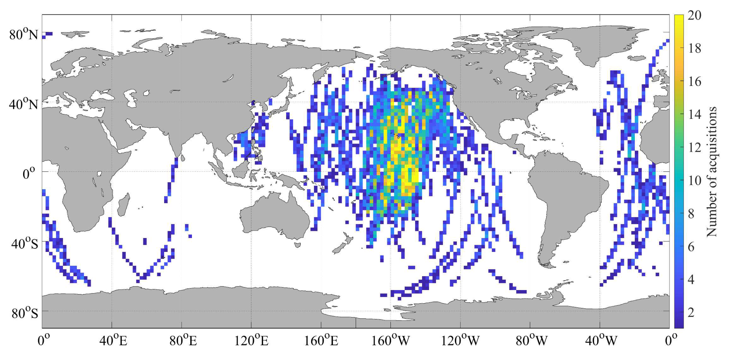
The Chinese Gaofen-3 satellite carrying a C-band (5.3 GHz) SAR sensor has been in orbit since August 2016. Gaofen-3 SAR can operate in 12 imaging modes, of which wave mode is dedicated to ocean wave detection. In wave mode, Gaofen-3 SAR collects small SAR images (called imagettes) with an approximate coverage of 5 km × 5 km every 50 km along the flight direction and a nominal spatial resolution of 4 m over the open ocean. It provides quad-polarimetric (HH (horizontal–horizontal)+HV (horizontal–vertical)+VH+VV) capability, and its incidence angle is designed to be capable of switching from 20° to 50° corresponding to 27 radar beams (denoted as ID, ranging from 189 to 216). In this paper, the Level-1A single-look complex (SLC) wave mode imagettes for the years from 2016 to 2020 were collected. The SAR scenes contaminated by non-wave phenomena were rejected, based on the following procedure: (1) The power saturated data were rejected by checking ‘echoSaturation’ value provided in the Gaofen-3 SAR product annotation file; (2) The imagettes contaminated by ice and land/island were excluded; (3) The homogeneity was checked, according to the method proposed by Schulz-Stellenfleth [26]. The percentage of rejection by the quality controls was approximately 30%, and finally, approximately 11200 Gaofen-3 SAR imagettes were selected in this study (Figure 1). 
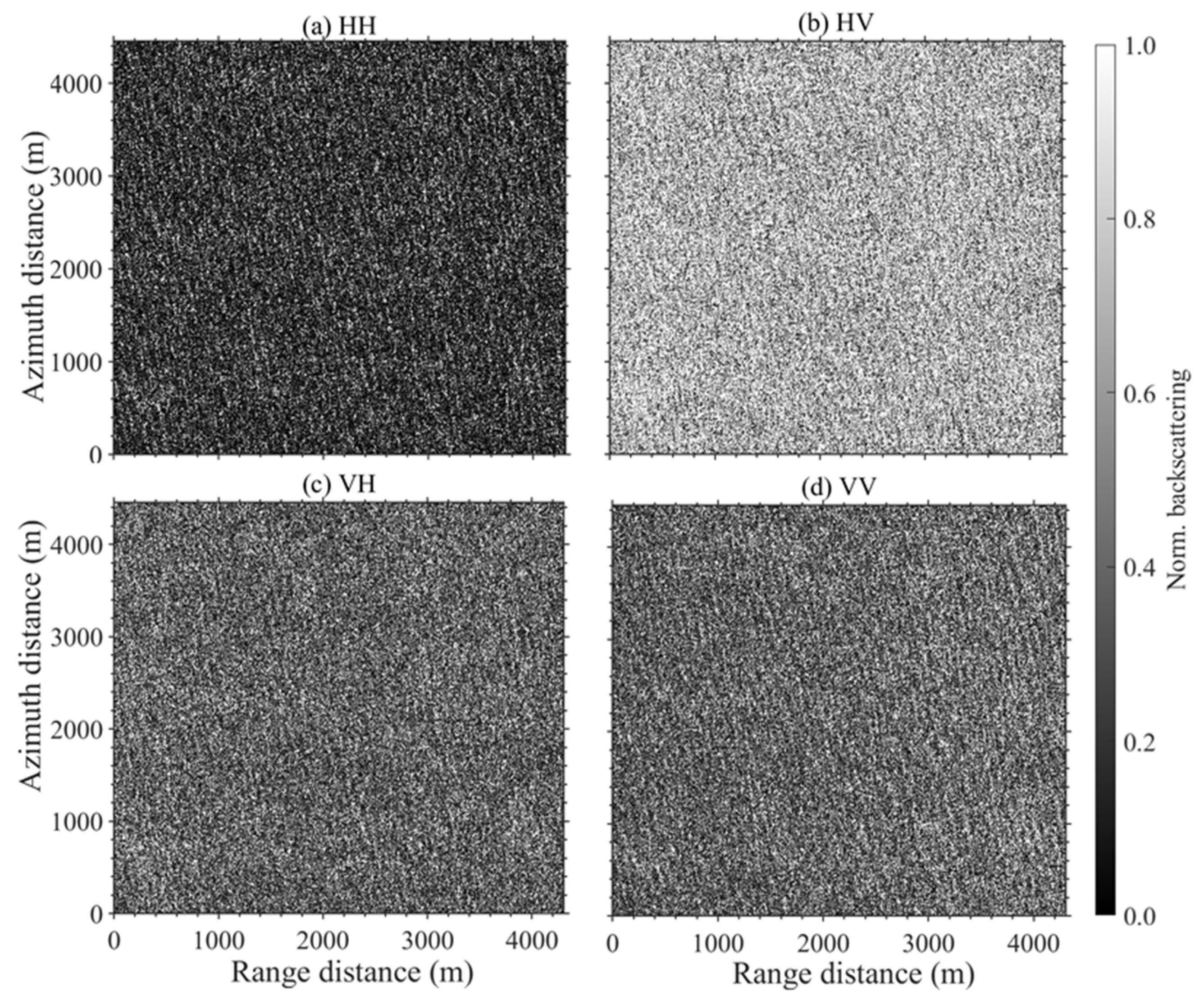
Figure 2 displays a typical example of the quad-polarization Gaofen-3 SAR imagettes, which was acquired on 7 February 2017, at 18:17 UTC. The images shown in Figure 2 were normalized by the min–max method, from which a clear wavy structure can be seen.
In the previous studies (e.g., [4,21,27]), the normalized radar cross-section (NRCS), the normalized image variance (cvar), and the azimuth cut-off wavelength (λc) were the three SAR features assumed to be strongly correlated with SWH, and they were most commonly used for SAR SWH inversion. In addition, the radar incidence angle (θ) was assumed to be an important parameter and has been considered for SAR SWH retrieval in recent studies. Therefore, in this paper, these four features were selected. The ways to extract these features are provided below.
(1) Normalized radar cross-section (NRCS)
The NRCS of the SAR image is typically related to the ocean surface wind, and thus, can represent information on short wave roughness [25]. The Gaofen-3 NRCS values at HH, HV, VH, and VV polarizations can be obtained by the following formula:
σ p q 0 = 10 log 10 D N p q K p q
where pq denotes the polarization state, σ0 is the NRCS in dB, <DNpq> denotes the mean value, DN = Is × (qv/32767)2 denotes the image intensity, Is = I2 + Q2 with I (Q) being the value of real (imaginary) channel for the single look complex SAR image, qv is the maximum qualified value stored in the product annotation file according to the polarizations, and K is the calibration constant also stored in the product annotation file according to the polarizations. However, only a small portion of the official Gaofen-3 wave mode products provide the quad-polarization 
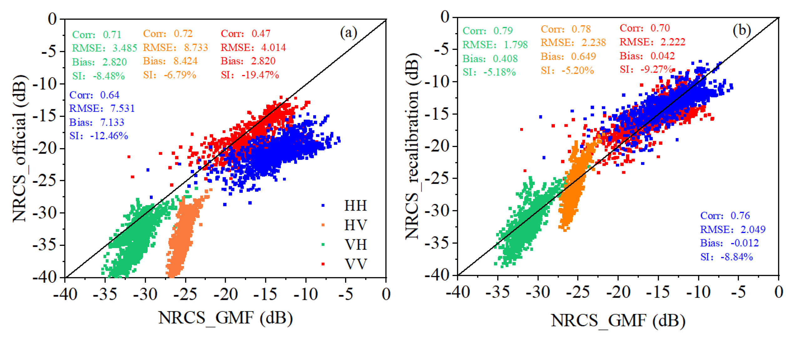
K values. Moreover, there are still some problems with the official radiometric calibration, though great efforts have been made. The comparisons of the Gaofen-3 NRCS values calibrated using the calibration constant of officially released values with those predicted by the empirical geophysical model functions (GMFs) at HH, HV, VH, and VV polarizations are shown in Figure 3a. The GMF CMOD5.n was used for VV; the combination of CMOD5.n and the VV-HH polarization ratio (PR) model proposed in Zhang et al. [27] was used for HH; and the C-3PO developed in Zhang et al. [28] was used for HV and VH. As seen, the calibrated NRCSs by the calibration constant of official released values significantly deviated from the GMF predictions with an RMSE up to ~4 dB, even in the best performing case of VV polarization. That is to say, extra calibration consideration and activity are needed to improve the accuracy of the Gaofen-3 SAR wave mode products.
This paper performs an ocean recalibration for the quad-polarization Gaofen-3 wave mode imagettes, based on the GMFs of CMOD5.n, CMOD5.n+PR, and C-3PO. The recalibration dataset was obtained by interpolating the 10-m height ocean winds from ERA5 at a 0.25° spatial and a 1-hour temporal resolution into the acquisition times and center locations of Gaofen-3 wave mode imagettes. For every imagette, the mean DN values at HH, HV, VH, and VV polarizations were computed by averaging all DN values within the corresponding 5 km × 5 km Gaofen-3 SAR images. The corresponding GMF-based NRCS values were computed using the collocated ERA5 winds. By correspondingly subtracting the GMF-predicted NRCS values (in dB) from the mean Gaofen-3 measured DN values (in dB), the new quad-polarization calibration constants were obtained for every imagette. Then, finally, 24 groups of quad-polarization recalibration constants were determined by averaging these new quad-polarization calibration constants within each Gaofen-3 radar beam (here, it was 24, not 27, since there were no imagettes in three radar beams with IDs of 192, 194, and 196 in the collected Gaofen-3 wave mode dataset). The values of the quad-polarization recalibration constants of the 24 Gaofen-3 radar beams are provided in Table A1 of Appendix A. Figure 3b shows the comparisons of the Gaofen-3 NRCS values calibrated using the ocean recalibration procedure with the GMF predictions at HH, HV, VH, and VV polarizations. It can be seen that the recalibrated NRCSs show good agreement with the GMF predictions.
(2) Normalized image variance
The normalized image variance (cvar) contains information on the sea state of longer waves. It is defined as the variance of the Gaofen-3 image normalized by the mean intensity:
c v a r p q = v a r ( D N p q D N p q D N p q )
where <DNpq> is the mean intensity of the pq polarization Gaofen-3 image in linear unit. In this study, the normalized variances for HH-, HV-, VH-, and VV-polarized wave mode images were considered.
(3) Azimuth cutoff
In the azimuth direction, SAR image processing relies on the backscattered signal phase analysis assuming a homogeneous and frozen surface to achieve high resolution. Over the ocean, according to the SAR-ocean imaging mechanism of velocity bunching, the surface wave motions may distort the phase history of the backscattered signal, leading to nonlinear transformation between the local wave and the SAR image. As a result, the small wave components propagating near the azimuth direction may be blurred. This leads to a cutoff value, where waves with wavelengths below the cutoff cannot be resolved by SAR. Using linear wave theory, the azimuth cutoff (λc), in meters, can be written as:
λ c = π β 0 ω 2 F ( f ) d f
where F is the wave spectrum, f is the wave frequency, ω = 2πf denotes the angular frequency, and β = R/V, with R being the satellite slant range and V being the satellite velocity. The magnitude of the spectral integration is directly related to the sea state conditions [23]. Therefore, the azimuth cutoff, normalized by the ratio of β, was chosen as another input parameter for our models. The azimuth cutoff can be estimated by fitting a Gaussian function to the inter-correlation of SAR cross-spectrum (real part) [29]. The Gaussian fit function C is stated as follows:
C ( x ) = exp ( ( π x λ c ) 2 )
where x denotes the spatial distance in the azimuth direction. 
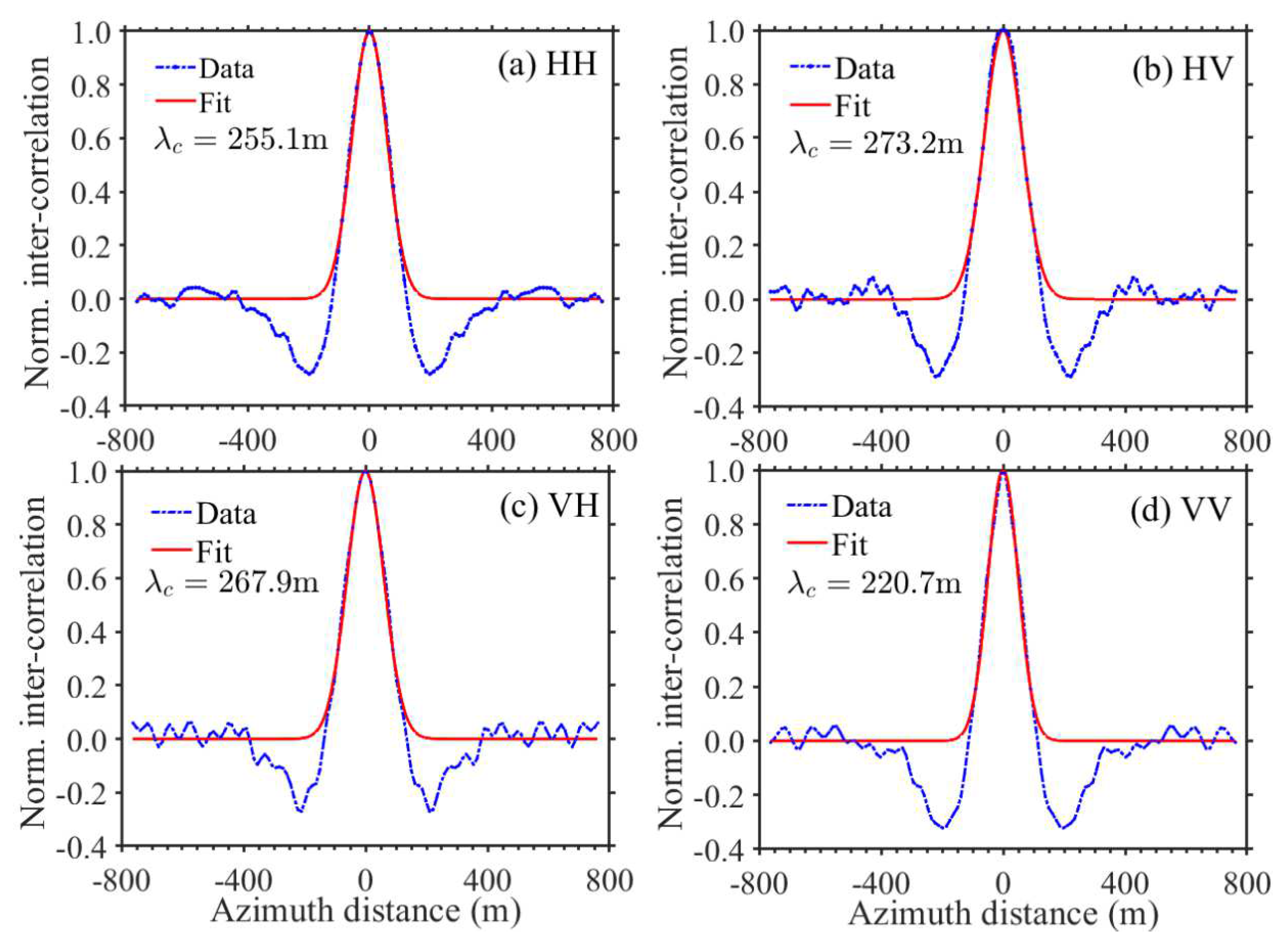
Figure 4 shows estimation of azimuth cutoff from the imagette shown in Figure 2 at polarization channels of HH, HV, VH, and VV. As seen, the values of the azimuth cutoff obtained from SAR images at different polarizations were different. The HV and VH cutoffs were larger than the HH and VV estimates. This is probably attributed to the fact that the smearing effects of cross-polarization SAR were larger for shorter coherence times [30]. The HH cutoff was slightly larger than the VV estimate. This may have been related to the larger HH-polarization modulation transfer function [30]. The azimuth cutoff estimates under HH, HV, VH, and VV configurations were considered in our models.
(4) Incidence angle
The incidence angle (θ) is an important parameter that should be considered when building empirical models for SAR SWH retrieval (e.g., [
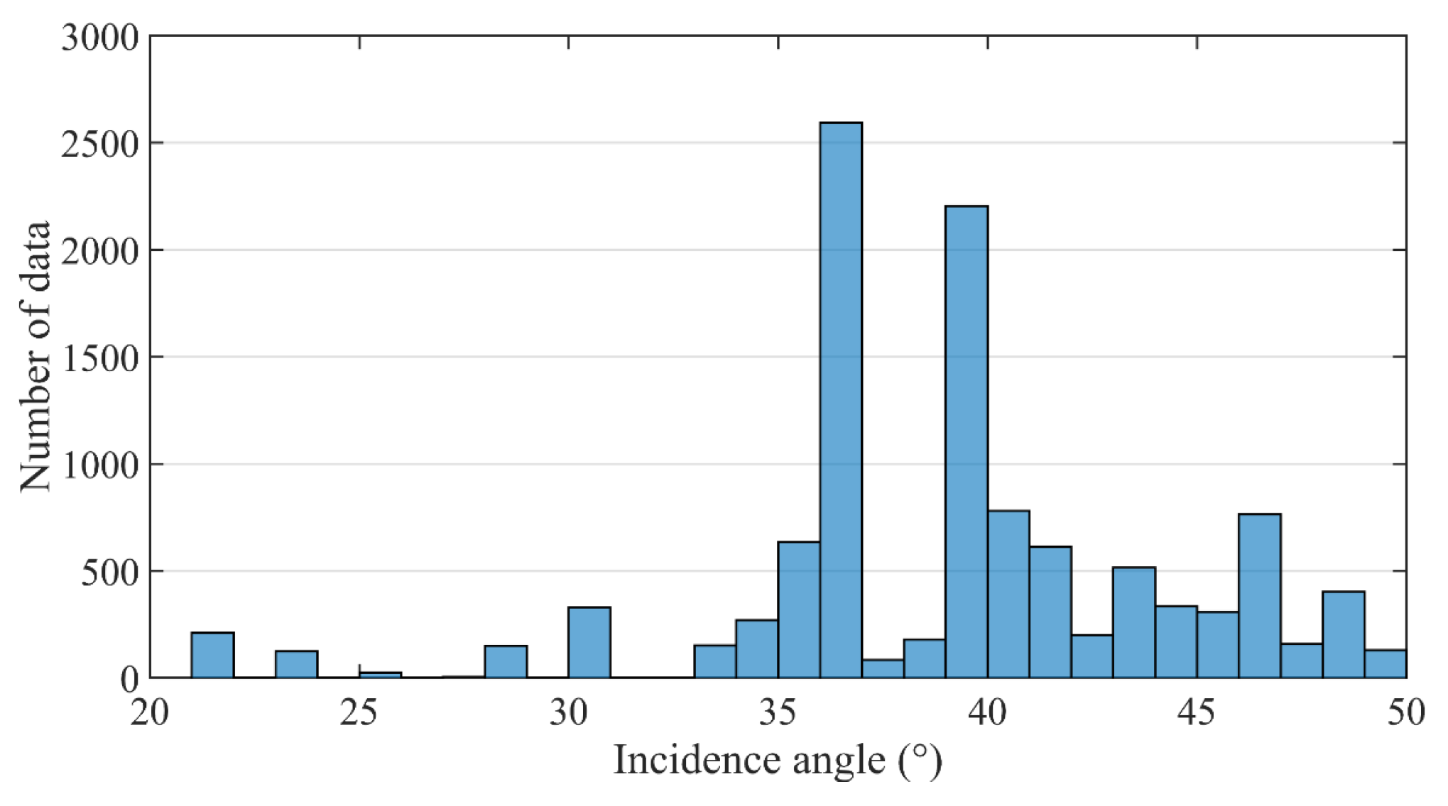
4]). Unlike the wave mode imagettes from European SAR satellites involving only one or two specific incidence angles, the incidence angle of Gaofen-3 wave mode could be switched from 20° to 50°. Figure 5 shows the histogram of incidence angles in 1° bin for Gaofen-3 wave mode data used in this study. As seen, the incidence angles were mostly distributed around 36° and 40°. Inspired by Wang H. et al. [24], and considering the amount of data, we categorized the Gaofen-3 wave mode data into five groups, with respect to incidence angle, called WV01 for 20–33°, WV02 for 33–37°, WV03 for 37–42°, WV04 for 42–46°, and WV05 for 46–50°. Details are listed in 
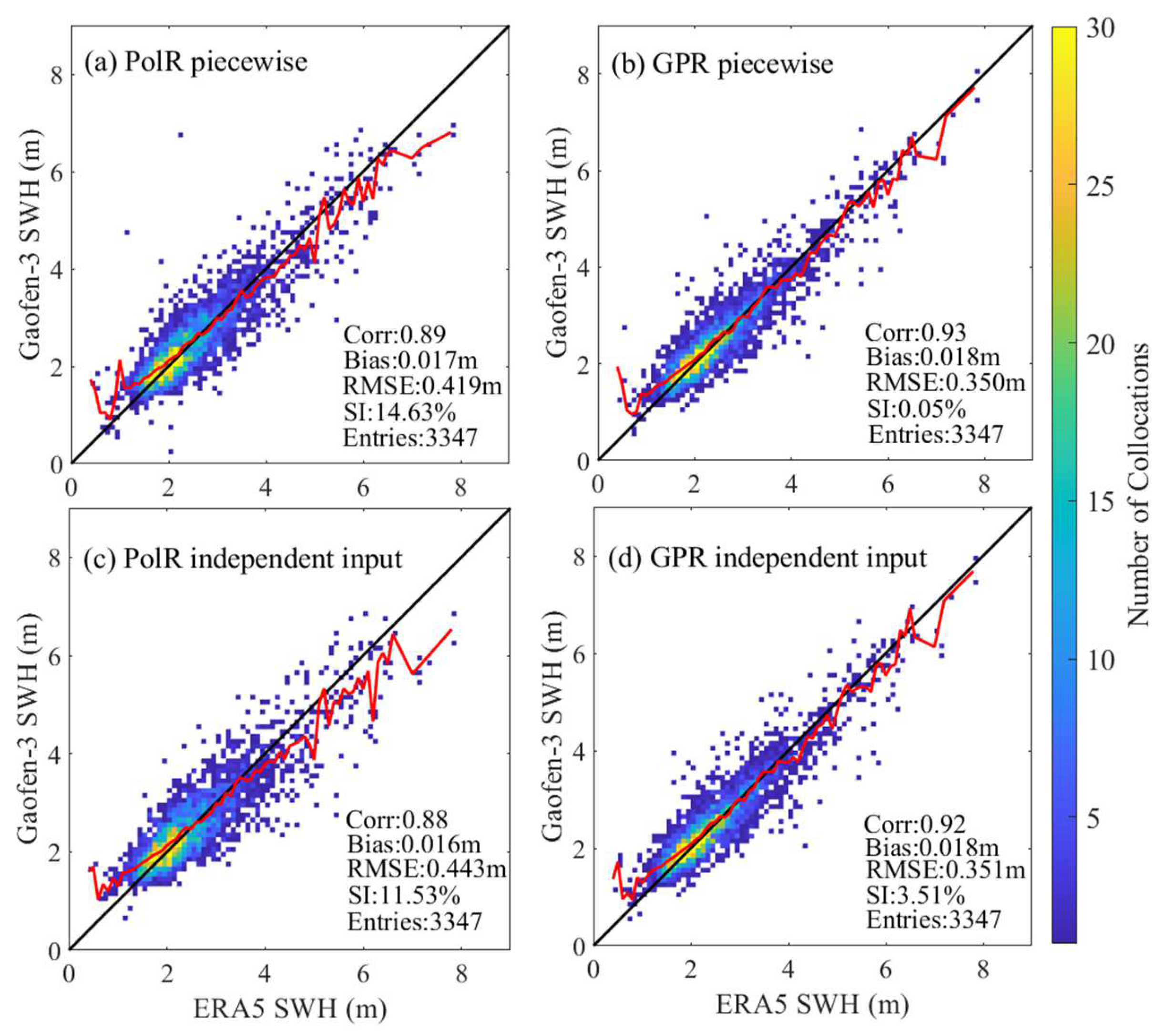
Table 1. The incidence angle range of WV01 was set so wide because of the small amount of data. The incidence angle was considered in two ways: first, it was included as an independent variable in the models, and second, the models were separately built at each incidence angle bin.

2.2. Buoy, Altimeter, and ERA5 SWH Data

The SWH observations from the standard meteorological data of the 61 moored buoys in the waters around the U.S., operated by the National Data Buoy Center (NDBC), were collected in this paper. All the buoys were located in the waters more than 50 km away from land and over 150 m deep in depth. The quality of the NDBC SWH observations was very high, with an accuracy of approximately 0.2 m [31]. The NDBC SWH observations were used as an independent data source to validate the derived SWH from the models. Besides, they were also used to assess the quality of the altimeter and ERA5 SWH data.
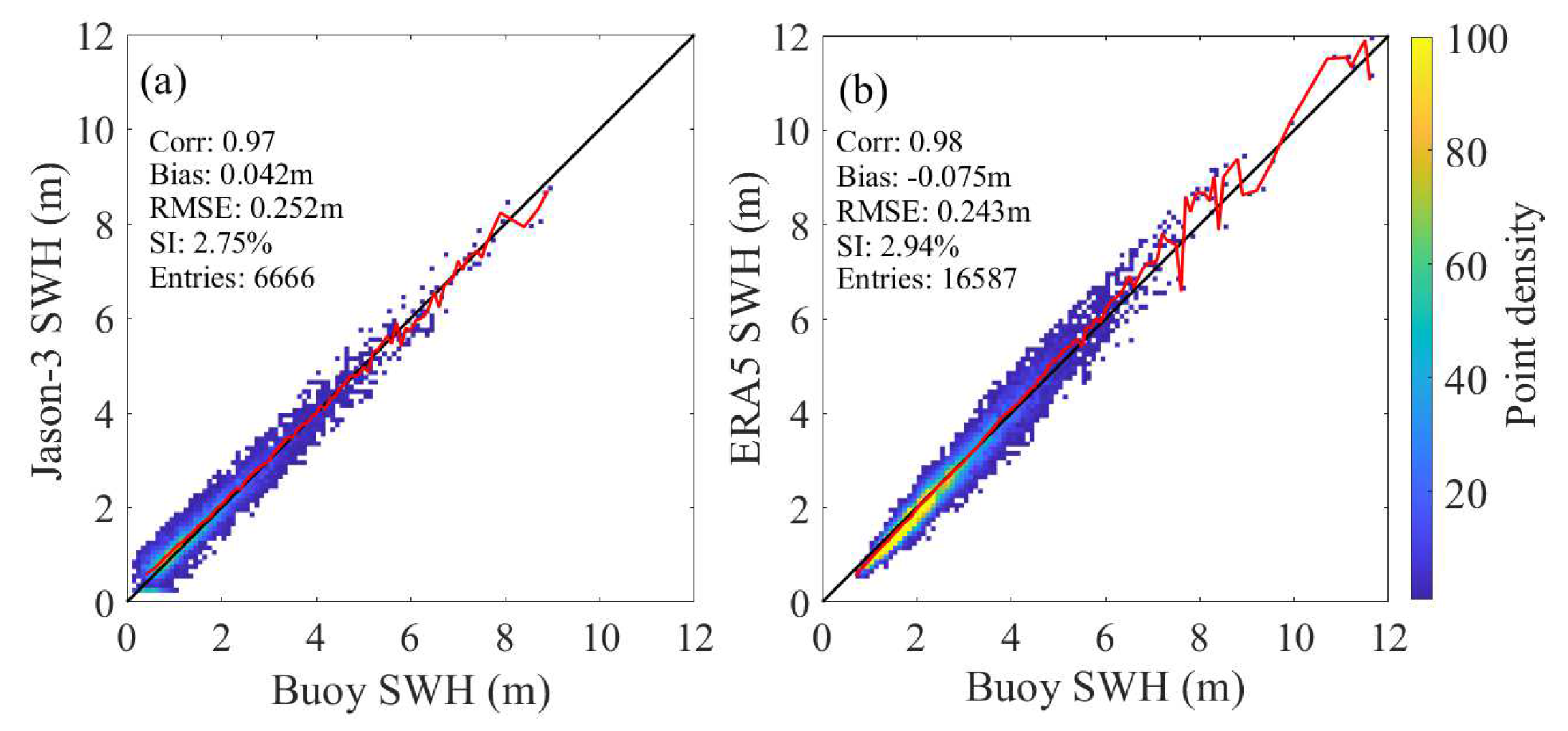
The SWH observations from Jason-3 altimetry mission were selected as an additional data source for the independent verification. The Jason-3 satellite was launched in January 2016 and carries a dual frequency (Ku- and C-bands) radar altimeter. The geophysical data records distributed by the Archiving, Validation, and Interpretation of Satellite Oceanographic Data (AVISO) for the period 2016–2020 were collected, and the SWHs retracted from Ku-band data were selected here. The Jason-3 SWH observations were recognized as being of good quality. The comparison between Jason-3 SWH and buoy SWH with correlation coefficient (Corr), root mean square error (RMSE), mean bias (Bias), and scattering index (SI) are shown in Figure 6a. As can be seen, the Jason-3 SWH observations were rather consistent with the buoy ones, with RMSE being about 0.252 m.
ERA5 is the fifth generation ECMWF atmospheric reanalysis for the global climate and weather [32]. It combines as many observations as possible into model estimates using advanced modeling techniques and latest data assimilation systems, and it provides new best estimates of the state of the atmosphere, ocean waves, and land surface. Compared to its predecessor, ERA-Interim, ERA5 has an improved temporal resolution as 6-hour in ERA-Interim to hourly in ERA5. The ERA5 hourly data on single levels published so far cover the period from 1 January 1950 to near real time. This dataset provides estimates for a number of ocean-wave variables at a regular lat-lon grid of 0.5 degrees, in which the significant height of combined wind waves and swell, i.e., SWH, are focused here. The accuracy of the ERA5 SWH was quantitatively assessed by comparing with the buoy observations. Figure 6b shows the comparison of ERA5 SWH with buoy SWH. As can be seen, the ERA5 SWH estimates were well-consistent with the corresponding buoy SWH observations, with RMSE being about 0.243 m.
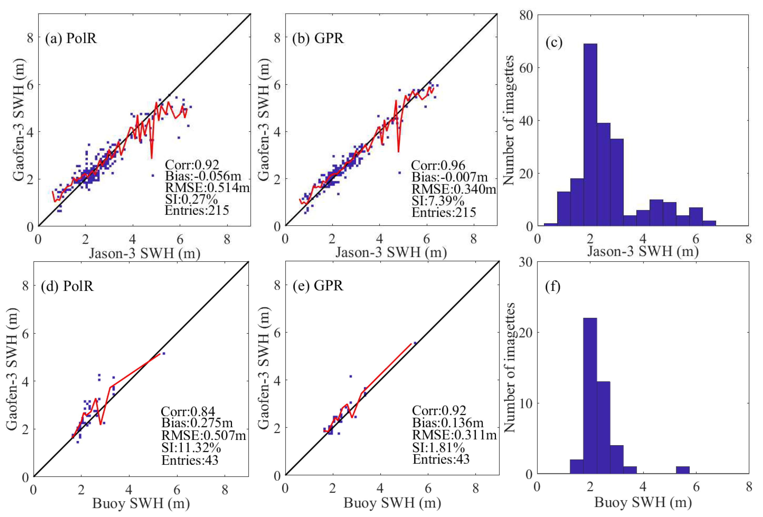
The Gaofen-3 SAR imagettes were collocated, respectively, with the NDBC buoy SWH observations and the Jason-3 altimeter SWH observations using the criteria of time separation within 1 h and spatial separation less than 100 km. This procedure yielded only 43 SAR-buoy matching points, of which, the buoy SWHs were mainly distributed 2–3 m. The collocation with Jason-3 yielded 215 points, of which, the Jason-3 SWHs were between 1–7 m. Each Gaofen-3 imagette was collocated with the time/space interpolated SWH from ERA5, yielding approximately 11,200 matched up cells, and the collocated ERA5 SWHs roughly ranged from 0.3 to 8 m. The collocations of Gaofen-3 SAR wave mode imagettes and ERA5 data were used to maximize the samples, since the collocations of SAR-buoy and SAR-altimeter were not sufficient for the model training. That is, the SAR-ERA5 data were used for the training of the PolR and GPR models. The SAR-buoy and SAR-altimeter data were never seen by the models when tuning to ensure an independent verification. The SAR-ERA5 data were randomly divided into two subsections for training (70% of the data) and for testing (30% of the data), both for the development of the models. The training set tuned the parameters of the PolR and GPR models, while the validation set cross-validated and determined the parameters. The effects of polarization and incidence angle on the models for estimating SWH from Gaofen-3 wave mode data were analyzed based the SAR-ERA5 data, as well.

2.3. PolR and GPR Models

The polynomial regression (PolR) model and the Gaussian process regression (GPR) model were adopted in this study for the multi-incidence angle polarimetric Gaofen-3 SAR SWH retrieval. The PolR model uses the basic formulation of the CWAVE model as:
H s = a 0 + i = 1 n a i × s i + i , j = 1 n a i , j × s i × s j
where Hs is the SWH, si represents the SAR-based parameters, and ai, j (ijn) represents the tuned coefficients. The PolR model states that the SWH is expressed as linear combinations of the SAR-derived parameters (s1, …, sn) with the extended coefficient vector (a0, …, an, a11, …, ann) in a dimension of 0.5 (n2 + 3n + 2). The second-order terms in the model function reflect the nonlinear combinations among the SAR image parameters. The derivation of the PolR model was based on the collocated Gaofen-3 SAR wave mode imagettes and ERA5 SWH data, using a least squares minimization procedure.
The GPR is a machine learning model with strong adaptability and good generalization ability for dealing with high dimensional nonlinear data. It is a flexible nonparametric Bayesian approach, using nonlinear mapping to relate the output to the input [33]. The salient feature of GPR is that it directly defines a prior probability over a latent function. The functional relationship of GPR is typically expressed in the form:
y = f ( X ) + ε
where y is the model output, X is the model input, ε is the independent identically distributed Gaussian noise with zero mean and constant variance, and f (X) is a Gaussian process that can be specified by its mean (which is taken to be zero) and covariance matrix K. The elements of K can be computed by using a kernel function. Several kernel functions were evaluated here, and it was found that the anisotropic exponential kernel was the most suitable. This exponential kernel function can be expressed as:
k ( x i , x j ) = θ 1 2 e x p ( - ( x i x j ) T ( x i x j ) θ 2 )
where k(xi, xj) is the (i, j) element of covariance matrix K, xi and xj are the ith and jth input parameters, and θ1 and θ2 represent hyper-parameters that should be optimized. In this work, the hyper-parameters of kernel function were estimated based on minimization of the negative log marginalized likelihood (NLML) [34]. To optimize the NLML, the quasi-newton optimization method was employed. The extracted features from the polarimetric Gaofen-3 SAR images were used as the input, and the ERA5 SWH was used as the training output. The inputs were transformed into the standardized values, so that the mean was 0 and the standard deviation was 1. Of particular note is that the GPR model does not need to include squared terms and cross-terms as input because it can model the nonlinear interactions between the input independent variables.

3. Results

In this section, the effects of polarization and incidence angle on the SWH estimation from multi-incidence angle quad-polarization Gaofen-3 SAR wave mode data using the PolR and GPR models were analyzed based on the SAR-ERA5 collocations. Then, the prediction accuracies of the final models were independently assessed based on the collocations of SAR-buoy and SAR-altimeter.

3.1. Effects of Polarization

Polarimetric SAR has shown significant advantages in SWH estimation, due to its richer backscattering information (e.g., [4,25]). Considering that how to make full use of SAR polarimetry information to achieve optimal SWH estimation is still an open question, the effects of polarization on the Gaofen-3 wave mode SAR SWH retrieval were further analyzed here, based on the collocated data set of approximately 12,000 quad-polarization Gaofen-3 imagettes matched with SWH from ERA5 by comparing the prediction accuracies of the PolR and GPR models under nine different polarization modes, including four single-polarization modes (HH, HV, VH, VV), four dual-polarization modes (HH+HV, VV+VH, HV+VH, HH+VV), and the quad-polarization mode (HH+HV+VH+VV). For this analysis, the recalibrated NRCS, cvar, and λc/β were used as inputs for the models. The θ was not considered. The training dataset and the validation dataset were kept unchanged in this experiment.
The performance of the PolR and GPR models in the nine polarization modes is recorded in Table 2. For both the PolR and GPR models, the four single-polarization modes performed similarly weaker, with lower correlation coefficients and higher RMSEs. Then, there were the dual-polarization modes of HH+VV and HV+VH, which showed slightly higher correlation coefficients and lower RMSEs. The dual-polarization modes of HH+HV and VV+VH had similarly stronger performance, with even higher correlation coefficients and lower RMSEs. The quad-polarization mode was the strongest, with the highest correlation coefficient and the lowest RMSE. Overall, the dual-polarization modes performed better than the single-polarization modes, and the quad-polarization mode performed better than the dual-polarization modes, indicating the more polarized content, the better performance of SAR SWH estimation. Note that HH, VV, and HH+VV are co-polarization channels; HV, VH, and HV+VH are cross-polarization channels, while HH+HV, VH+VV, and HH+HV+VH+VV are hybrid polarization channels. The hybrid polarization has stronger performance than the co-polarization or the cross-polarization alone. This is probably due to the fact that the combination of co-polarization and cross-polarization can work effectively over the whole sea state, as the co-polarization only works at low to moderate seas, while the cross-polarization works at high seas [4]. In addition, one can see that the performance of PolR model was obviously weaker than that of GPR model. The RMSEs of PolR model were approximately 0.1 m larger than the corresponding GPR ones. This suggests that the added nonlinearity of the Gaussian process regression was able to model SWH more accurately than the polynomial regression.
Taking the GPR model as an example, the performance of Gaofen-3 SWH estimation at different sea states under the nine polarization modes was illustrated to demonstrate further the advantages of multi-polarization, especially hybrid polarization, in SAR SWH retrieval. Similar results were obtained for PolR. Figure 7 shows the plots of Gaofen-3 SWH retrievals from GPR against ERA5 SWH, independent of the model training process (validation dataset) for the nine polarization modes. The solid red lines represent the mean values of SAR retrievals in each 0.1 m bin of ERA5 SWH. Figure 8a–c display the dependency of the SWH residuals (GPR estimates minus ERA5 SWH) against ERA5 SWH over the range from 0 m to 8 m, stepped by 1 m at the nine polarization modes. Figure 8d shows the histogram of ERA5 SWH in a bin size of 1 m.
One can see from Figure 7 and Figure 8 that, for all the polarization modes, reasonably good SWH estimates were archived via the GPR model under moderate sea conditions (roughly 1–4 m), where the mean lines almost overlapped the one-to-one straight line, and the residuals were close to zero. This probably resulted from two reasons: (1) both co-polarization and cross-polarization work well at moderate sea states; (2) the data were mostly distributed in moderate seas. However, overestimation/underestimation could be found under low/high sea conditions. Compared to the co-polarization modes, such as HH, VV, and HH+VV, the cross-polarization modes, such as HV, VH, and HV+VH, showed larger overestimation in low wave regime, but smaller underestimation in high wave regime. This implies that the co-polarization/cross-polarization can benefit SWH estimation under low/high sea conditions. The hybrid polarization modes, such as HH+HV, VV+VH, and HH+HV+VH+VV, achieved better performance by combining the advantages of co-polarization and cross-polarization. Their mean lines were closer to the one-to-one straight line, and their residuals were closer to zero over the whole SWH range. In addition, it can be seen that the dual-co-polarization performed better than HH or VV alone; the dual-cross-polarization performed better than HV or VH alone; the quad-polarization performed better than the dual-hybrid polarizations. That is to say, the performance of Gaofen-3 SWH inversion improved, as long as polarimetry information increased, which further demonstrates the enhancement effect of multi-polarization on SAR SWH retrieval. However, the improvement was found to not be considerable in low to moderate seas (about < 4 m), when dual-polarized information or even quad-polarized information were exploited. This implicates that single-polarized SAR data are sufficient for accurately retrieving SWH under low-moderate sea states.

3.2. Effects of Incidence Angle

The quad-polarization PolR and GPR models were tuned and tested, respectively, for each of the five incidence angle bins (see Table 1 for details), based on the training and validation datasets used in Section 3.1, which were subdivided into five incidence angle bins separately, to explore the dependence of Gaofen-3 SWH retrieval on incidence angle. Table 3 shows the error metrics for the quad-polarization PolR and GPR models under different incidence angle bins. In general, both PolR and GPR models performed differently across different incidence angle bins. They had better performance at lower incidence angles than at higher incidence angles, which may reveal that lower incidence angles are more favorable for SAR SWH inversion. This is possibly owing to the higher signal-to-noise ratio and the stronger tilt modulation at lower incidence angles [15]. However, it should also be noted that WV03 (θ around 40°) outperformed WV02 (θ around 35°). This occurred in the research of Wang et al. [24], as well. It may imply that the Gaofen-3 radar beams within WV03 enable relatively high-quality imaging. In addition, it is worth mentioning that the quad-polarization PolR model performed better than the QPCWAVE_GF3 model proposed in [24], which used a similar formulation, but only additionally introduced VH NRCS, besides the VV features. This further confirms the necessity of fully exploiting the quad-polarized information.
There are two ways to introduce incidence angles in the PolR and GPR models. First, as the above, the Gaofen-3 SAR wave mode data were categorized into five groups, with respect to incidence angle, and piecewise functions were created for the PolR and GPR models. Second, the incidence angle was used as one of the independent inputs to the PolR and GPR models. It should be noted that the same training and validation datasets as Section 3.1 were adopted here. Figure 9 displays the scatter plots of Gaofen-3 SWH retrievals from (a) the piecewise quad-polarization PolR model, (b) the piecewise quad-polarization GPR model, (c) the quad-polarization PolR model that included θ as an independent variable, and (d) the quad-polarization GPR model that included θ as an independent variable against independent ERA5 SWH. It was found that the quad-polarization models showed obvious improvement in performance when θ was additionally considered, particularly in the piecewise way. The piecewise models from the incidence angle bins performed slightly stronger than the corresponding models that included θ as an independent variable, especially for the PolR model and at high sea states. The impact of the ways to consider θ on the performance of the GPR model was rather little.

3.3. Final Model Performance

To sum up, with the input scheme that included the quad-polarized features and introduced the incidence angle in a piecewise way, the PolR and GPR models achieved superior performance for SWH inversion from the Gaofen-3 wave mode data. The final optimal PolR and GPR models were independently assessed here by comparing their predictions with measurements from the Jason-3 altimeter and NDBC buoys. Figure 10 presents the scatter plots of Gaofen-3 SWH retrievals from the final PolR and GPR models against the SWH measurements from Jason-3 altimeter and NDBC buoys. The final PolR model achieved an RMSE of 0.514 m, compared to altimeter data, showing almost no reduction in RMSE from QPCWAVE_GF3 in [24] of 0.52 m. The expected optimizations did not significantly occur, possibly due to the large uncertainty in the validation data set, caused by the small amount of altimeter collocations (only 215). The final GPR model achieved 0.34 m RMSE, compared to the altimeter data, which was close to that of GF3WVResNet_QP (0.32 m), a more complex, deep convolutional network-based SAR SWH retrieval algorithm in quad-polarization proposed in [4] and the previous state-of-the-art algorithm for estimating SWH from Gaofen-3 wave mode data. The final GPR model even achieved a higher correlation coefficient (0.94 to 0.96), lower bias (0.05 m to -0.01 m), and lower SI (12.59% to 7.39%). On the test set of 43 buoy collocations, the final PolR and GPR models, respectively, achieved RMSEs of 0.507 m and 0.311 m. The errors on the buoy data set were smaller because the buoys tend to be located in the waters where there are more moderate sea states and smaller errors. For both models, the mean lines had slopes less than 1, which reflects that the models overestimated small SWH (< 2 m) and underestimated large SWH (> 6 m). In addition, the final GPR model, with nearly 0.2 m lower RMSE, outperformed the final PolR model.

4. Discussion

4.1. Importance Study of the Polarization Features

From Section 3.1, one can conclude that the hybrid polarization had obvious advantages in Gaofen-3 SAR SWH estimation. However, it remains questionable whether all input polarization features could cause the polarization enhancement. Therefore, feature importance studies were performed here for the PolR and GPR models developed in Section 3.1 (θ was not considered), under the hybrid polarization modes of HH+HV, VV+VH and HH+HV+VH+VV. For each of the hybrid polarization modes, additional models were trained with one of the input features removed and other features unchanged. Table 4 shows the error metrics for the PolR and GPR models, with different input features removed under the polarization mode of HH+HV. Table 5 shows the VV+VH case. The quad-polarization case is provided in Table 6. For both dual-hybrid polarization modes, degradation in performance can be seen when removing any one of the input features, suggesting that every feature contains additional information that is relevant to predicting SWH, given the other inputs. For both PolR and GPR models, the degradation caused by NRCS and cvar was larger than that caused by λc. The largest reduction in error could be seen when removing the cross-polarization NRCS, which was not unexpected, as it can represent information on wind-sea energy under extreme wind/wave conditions, where saturation is observed in co-polarization. The removal of cross-polarization λc causes the smallest reduction in error. For the quad-polarization mode, most of the input features caused similar, albeit smaller, degradation. Additionally, the effects of NRCS and cvar were generally larger than that of λc, particularly the cross-polarization NRCS. The cross-polarization λc showed very small effects. It even showed slight side effects for the GPR model. In addition, for the PolR model, the cross-polarization cvar also conveyed no useful information. The small or side effects of cross-polarization λc and cvar possibly resulted from the low signal-to-noise ratio of the cross-polarization SAR images.

4.2. Impact of Radiometric Calibration

As is known, high-precision SAR wind estimation depend highly on the good quality of NRCS, mainly resulting from the accurate absolute radiometric calibration of the SAR imagery. The fact that the radiometric calibration has a great impact on SAR wind retrieval has been widely demonstrated [35]. For SAR SWH retrieval, the specific impact of radiometric calibration is still not well-understood, although previous studies have pointed out that proper calibration of NRCS is necessary, in order to accurately estimate SWH from SAR (e.g., [35]). Considering that Gaofen-3 SAR has problems in radiometric calibration, its impact on Gaofen-3 SAR SWH retrieval is discussed here, based on the 4576 imagettes that provide official calibration constants through comparing the performance of the PolR and GPR models with inputs of different NRCS-related parameters—the recalibrated NRCS ( σ r e c a l 0 ), the officially calibrated NRCS ( σ o f f i c i a l 0 ), the mean DN in dB ( 10 log 10 D N ), or the mean Is in dB ( 10 log 10 I s ). The polarization modes of HH, HH+HV, and HH+HV+VH+VV were taken as examples for this discussion. The cvar and λ c / β were included in the models, while θ was not.
The performances of the PolR and GPR models with σ r e c a l 0 , σ o f f i c i a l 0 , 10 log 10 D N , or 10 log 10 I s inputs at the polarization modes of HH, HH+HV, and HH+HV+VH+VV are summarized in Table 7, Table 8 and Table 9. It should be mentioned that both the training data set used to create the models and the validation data set used to validate the models remain the same in the experiment, and thus, we expect the sampling to have no impact on the resulting model functions. It can be seen that the radiometric calibration improved the performance of Gaofen-3 SWH inversion for both PolR and GPR models under all the polarization modes of HH, HH+HV, and HH+HV+VH+VV, with RMSE reducing by about 0.1 m, due to the accurate radiometric calibration. This also implies that the impact of radiometric calibration does not decrease with the increase of polarimetry information. Furthermore, it is worth pointing out that, for both the PolR and GPR models, especially for the GPR model, the introduction of qv (from 10 log 10 I s to 10 log 10 D N ) brings about significant improvement. In addition, both the PolR and GPR models showed better performance with K set to the recalibration value (Krecal) than to the official calibration value (Kofficial), indicating that ocean recalibration is necessary for the accurate estimation of SWH from Gaofen-3 wave mode data.

5. Conclusions

At first, the effects of the polarization and incidence angles on Gaofen-3 SAR SWH inversion were systematically explored using the PolR and GPR models by comparing their prediction accuracies under different input schemes, based on the collocated data set of approximately 12,000 multi-incidence angle quad-polarization Gaofen-3 wave mode imagettes matched with SWH from ERA5 reanalysis. The SAR polarimetry information has great potential for accurately estimating SWH. For both the PolR and GPR models, the quad-polarization mode performed better than the dual-polarization modes, which were better than the single-polarization modes, i.e., the more polarized content, the better performance of SAR SWH estimation. Moreover, the hybrid polarizations that combined the channels of co-polarization and cross-polarization had stronger performance than the co-polarization or the cross-polarization alone, as they could work effectively over the whole sea state. Incidence angle also had effects on the model performance. The lower incidence angles were more favorable for SAR SWH inversion for the higher signal-to-noise ratio and stronger tilt modulation. Additionally, compared to the models that include incidence angle as an independent variable, the piecewise models from the incidence angle bins performed slightly stronger, especially for the PolR model and at high sea states.
Then, the final PolR and GPR models with the superior input scheme that included the quad-polarized features and introduced the incidence angle in a piecewise way were independently assessed by comparing their predictions with SWH measurements from Jason-3 altimeter and NDBC buoys. The final PolR model was slightly more accurate than the previously published model of QPCWAVE_GF3, which used a similar formulation, but only additionally introduced VH NRCS, besides the VV features. The final GPR model almost achieved the accuracy of GF3WVResNet_QP, which was previously a state-of-the-art, deep convolutional network-based, and more complex SAR SWH retrieval algorithm in quad-polarization. In general, the GPR model outperformed the PolR model, possibly owing to the fact that the added nonlinearity of GPR was able to model SWH more accurately than PolR.
Finally, we discussed the importance of polarization features and the impact of radiometric calibration on the Gaofen-3 SAR SWH estimation using the PolR and GPR models. For both dual-hybrid polarization modes, degradation in performance could be seen when removing any one of the input features, suggesting that every feature contained additional information that was relevant to predicting SWH, given the other inputs. For both PolR and GPR, the degradation caused by NRCS and cvar was larger than that of λc. The radiometric calibration improved the performance of Gaofen-3 SWH inversion. Notwithstanding our results, they were based on a fairly limited range of SWH. The data available for collection was concentrated below 8 m. There were no significant wave heights greater than 10 m, which are associated with extreme weather. Thus, we intend to continue to investigate our models for higher wind/wave conditions.

Author Contributions

Conceptualization, C.F. and Q.Y.; methodology, T.S.; software, T.S.; validation, Y.W., J.M. and J.Z.; writing—original draft preparation, C.F.; writing—review and editing, Q.Y.; funding acquisition, J.Z. All authors have read and agreed to the published version of the manuscript.

Funding

This research was funded by National Natural Science Foundation of China (NSFC), grant number 61931025, by the Key Program of Joint Fund of the National Natural Science Foundation of China and Shandong Province under, grant U2006207, and by the Fund of Technology Innovation Center for Ocean Telemetry, Ministry of Natural Resources, under grant JZ-06-1142.

Data Availability Statement

Not applicable.

Acknowledgments

The authors would like to thank Chinese National Satellite Ocean Application Service (NSOAS) for providing the Gaofen-3 SAR wave mode data via the website of https://osdds.nsoas.org.cn/, accessed on 7 October 2022, (registration required). The authors would also like to thank the American National Oceanic and Atmospheric Administration (NOAA) NDBC for providing the buoy data, thank AVISO for providing the Jason-3 altimeter data, and thank ECMWF for providing the ERA5 reanalysis data.

Conflicts of Interest

The authors declare no conflict of interest.

Appendix A

Table A1. The values of the quad-polarization recalibration constants of the 24 Gaofen-3 radar beams.
Radar Beam IDHHHVVHVV
18915.0140812.254125.8099120.05543
19018.2558514.8836829.1531820.59579
19118.8395316.6437624.8427619.13042
19321.2673517.9847625.4941720.49475
19526.7255522.7052426.2077420.39201
19728.259223.8421528.2124422.28621
19823.3218319.9801126.9885822.41353
19925.6507921.6770626.6751821.47405
20030.3013525.6382828.9566922.93642
20125.406921.2409826.0370120.61089
20229.1056423.9626528.5708122.89158
20329.1056423.9626528.5708122.89158
20530.6235225.3101829.4009623.89272
20629.1905723.5511527.6960522.62887
20729.5264323.6163627.1998321.79812
20829.2208723.1551927.5249122.39281
20929.1905123.2953228.8177823.13645
21028.8810522.176127.6476422.71903
21128.1835822.0620326.7279221.29466
21230.9004625.1070429.3956624.53799
21330.0509124.1300428.6303624.10765
21430.0509124.1300428.6303624.10765
21530.0509124.1300428.6303624.10765
21630.0509124.1300428.6303624.10765

References

  1. Hasselmann, K.; Raney, R.K.; Plant, W.J.; Alpers, W.; Shuchman, R.A.; Lyzenga, D.R.; Rufenach, C.L.; Tucker, M.J. Theory of synthetic aperture radar ocean imaging: A MARSEN view. J. Geophys. Res. Ocean. 1985, 90, 4659–4686. [Google Scholar] [CrossRef]
  2. Pramudya, F.S.; Pan, J.; Devlin, A.T. Estimation of significant wave height of near-range traveling ocean waves using Sentinel-1 SAR images. IEEE J. Sel. Top. Appl. Earth Observ. Remote Sens. 2019, 12, 1067–1075. [Google Scholar] [CrossRef]
  3. Alpers, W.R.; Bruening, C. On the relative importance of motion-related contributions to the SAR imaging mechanism of ocean surface waves. IEEE Trans. Geosci. Remote Sens. 1986, GE-24, 873–885. [Google Scholar] [CrossRef]
  4. Wang, H.; Yang, J.; Lin, M.; Li, W.; Zhu, J.; Ren, L.; Cui, L. Quad-polarimetric SAR sea state retrieval algorithm from Chinese Gaofen-3 wave mode imagettes via deep learning. Remote Sens. Environ. 2022, 273, 1–15. [Google Scholar] [CrossRef]
  5. Hasselmann, K.; Hasselmann, S. On the nonlinear mapping of an ocean wave spectrum into a synthetic aperture radar image spectrum and its inversion. J. Geophys. Res. Ocean. 1991, 96, 10713–10729. [Google Scholar] [CrossRef]
  6. Hasselmann, S.; Brüning, C.; Hasselmann, K.; Heimbach, P. An improved algorithm for the retrieval of ocean wave spectra from synthetic aperture radar image spectra. J. Geophys. Res. Ocean. 1996, 101, 16615–16629. [Google Scholar] [CrossRef]
  7. Engen, G.; Johnsen, H. SAR-ocean wave inversion using image cross spectra. IEEE Trans. Geosci. Remote Sens. 1995, 33, 1047–1056. [Google Scholar] [CrossRef]
  8. Mastenbroek, C.; De Valk, C.F. A semiparametric algorithm to retrieve ocean wave spectra from synthetic aperture radar. J. Geophys. Res. Ocean. 2000, 105, 3497–3516. [Google Scholar] [CrossRef]
  9. Schulz-Stellenfleth, J.; Lehner, S.; Hoja, D. A parametric scheme for the retrieval of two-dimensional ocean wave spectra from synthetic aperture radar look cross spectra. J. Geophys. Res. Ocean. 2005, 110, 1–17. [Google Scholar] [CrossRef] [Green Version]
  10. Sun, J.; Guan, C. Parameterized first-guess spectrum method for retrieving directional spectrum of swell-dominated waves and huge waves from SAR images. Chin. J. Oceanol. Limn. 2006, 24, 12–20. [Google Scholar]
  11. Schuler, D.L.; Lee, J.S.; Kasilingam, D.; Pottier, E. Measurement of ocean surface slopes and wave spectra using polarimetric SAR image data. Remote Sens. Environ. 2004, 91, 198–211. [Google Scholar] [CrossRef]
  12. Zhang, B.; Perrie, W.; He, Y. Validation of RADARSAT-2 fully polarimetric SAR measurements of ocean surface waves. J. Geophys. Res. Ocean. 2010, 115, 1–11. [Google Scholar] [CrossRef]
  13. Schulz-Stellenfleth, J.; Koenig, T.; Lehner, S. An empirical approach for the retrieval of integral ocean wave parameters from synthetic aperture radar data. J. Geophys. Res. Ocean. 2007, 112, 3019–3033. [Google Scholar] [CrossRef]
  14. Li, X.; Lehner, S.; Bruns, T. Ocean wave integral parameter measurements using Envisat ASAR wave mode data. IEEE Trans. Geosci. Remote Sens. 2011, 49, 155–174. [Google Scholar] [CrossRef] [Green Version]
  15. Stopa, J.E.; Mouche, A. Significant wave heights from Sentinel-1 SAR: Validation and applications. J. Geophys. Res. Ocean. 2017, 122, 1827–1848. [Google Scholar] [CrossRef] [Green Version]
  16. Ren, L.; Yang, J.; Zheng, G.; Wang, J. Significant wave height estimation using azimuth cutoff of C-band RADARSAT-2 single-polarization SAR images. Acta Oceanol. Sin. 2015, 34, 93–101. [Google Scholar] [CrossRef]
  17. Grieco, G.; Lin, W.; Migliaccio, M.; Nirchio, F.; Portabella, M. Dependency of the Sentinel-1 azimuth wavelength cut-off on significant wave height and wind speed. Int. J. Remote Sens. 2016, 37, 5086–5104. [Google Scholar] [CrossRef]
  18. Yang, J.S.; Ren, L.; Wang, J. The first quantitative remote sensing of ocean surface waves by Chinese GF-3 SAR satellite. Oceanol. Limnol. Sin. 2017, 48, 207–209. [Google Scholar]
  19. Sheng, Y.; Shao, W.; Zhu, S.; Sun, J.; Yuan, X. Validation of significant wave height retrieval from co-polarization Chinese Gaofen-3 SAR imagery using an improved algorithm. Acta Oceanol. Sin. 2016, 37, 1–10. [Google Scholar] [CrossRef]
  20. Shao, W.; Ding, Y.; Li, J.; Gou, S.; Nunziata, F.; Yuan, X.; Zhao, L. Wave retrieval under typhoon conditions using a machine learning method applied to Gaofen-3 SAR imagery. Can. J. Remote Sens. 2019, 45, 723–732. [Google Scholar] [CrossRef]
  21. Quach, B.; Glaser, Y.; Stopa, J.E.; Mouche, A.A.; Sadowski, P. Deep learning for predicting significant wave height from synthetic aperture radar. IEEE Trans. Geosci. Remote Sens. 2021, 59, 1859–1867. [Google Scholar] [CrossRef]
  22. Wu, K.; Li, X.; Huang, B. Retrieval of ocean wave heights from spaceborne SAR in the Arctic Ocean with a neural network. J. Geophys. Res. Ocean. 2021, 126, 6946. [Google Scholar] [CrossRef]
  23. Pramudya, F.S.; Pan, J.; Devlin, A.T.; Lin, H. Enhanced estimation of significant wave height with dual-polarization Sentinel-1 SAR imagery. Remote Sens. 2021, 13, 124. [Google Scholar] [CrossRef]
  24. Wang, H.; Wang, J.; Yang, J.; Ren, L.; Zhu, J.; Yuan, X. Empirical algorithm for significant wave height retrieval from wave mode data provided by the Chinese satellite Gaofen-3. Remote Sens. 2018, 10, 363. [Google Scholar] [CrossRef] [Green Version]
  25. Collins, M.J.; Ma, M.; Dabboor, M. On the effect of polarization and incidence angle on the estimation of significant wave height from SAR data. IEEE Trans. Geosci. Remote Sens. 2019, 57, 4529–4543. [Google Scholar] [CrossRef]
  26. Schulz-Stellenfleth, J.; Lehner, S. Measurement of 2-D sea surface elevation fields using complex synthetic aperture radar data. IEEE Trans. Geosci. Remote Sens. 2004, 42, 1149–1160. [Google Scholar] [CrossRef]
  27. Zhang, B.; Perrie, W.; He, Y. Wind speed retrieval from RADARSAT-2 quad-polarization images using a new polarization ratio model. J. Geophys. Res. Ocean. 2011, 116, 1–13. [Google Scholar] [CrossRef]
  28. Zhang, G.; Li, X.; Perrie, W.; Hwang, P.A.; Zhang, B.; Yang, X. A hurricane wind speed retrieval model for C-band RADARSAT-2 cross-polarization ScanSAR images. IEEE Trans. Geosci. Remote Sens. 2017, 55, 4766–4774. [Google Scholar] [CrossRef]
  29. Kerbaol, V.; Chapron, B.; Vachon, P.W. Analysis of ERS-1/2 synthetic aperture radar wave mode imagettes. J. Geophys. Res. Ocean. 1998, 103, 7833–7846. [Google Scholar] [CrossRef]
  30. Li, H.; Mouche, A.; Wang, H.; Stopa, J.E.; Chapron, B. Polarization dependence of azimuth cutoff from quad-pol SAR images. IEEE Trans. Geosci. Remote Sens. 2019, 57, 9878–9887. [Google Scholar] [CrossRef]
  31. National Data Buoy Center. Handbook of Automated Data Quality Control Checks and Procedures; NOAA National Data Buoy Center Tech, Stennis Space Center: Hancock County, MS, USA, 2009. [Google Scholar]
  32. Hersbach, H.; Bell, B.; Berrisford, P.; Hirahara, S.; Thépaut, J. The ERA5 global reanalysis. Q. J. Roy. Meteor. Soc. 2020, 146, 1999–2049. [Google Scholar] [CrossRef]
  33. Brahim-Belhouari, S.; Bermak, A. Gaussian process for nonstationary time series prediction. Comput. Stat. Data Anal. 2004, 7, 705–712. [Google Scholar] [CrossRef]
  34. Zhou, X.; Zhou, F.; Naseri, M. An insight into the estimation of frost thermal conductivity on parallel surface channels using kernel based GPR strategy. Sci. Rep. 2021, 11, 1–11. [Google Scholar] [CrossRef] [PubMed]
  35. Wang, H.; Li, H.; Lin, M.; Zhu, J.; Wang, J.; Li, W.; Cui, L. Calibration of the copolarized backscattering measurements from Gaofen-3 synthetic aperture radar wave mode imagery. IEEE J. Sel. Top. Appl. Earth Observ. 2019, 12, 1748–1762. [Google Scholar] [CrossRef]
Figure 1. Map of the selected Gaofen-3 wave mode acquisitions during the years 2016–2020 in data density for 2° × 2° bins.
Remotesensing 14 05480 g001
Figure 2. Case of Gaofen-3 SAR wave mode imagette, acquired on February 7, 2017, at UTC 18:17:16. Image of normalized backscattering for (a) HH, (b) HV, (c) VH, and (d) VV polarizations.
Remotesensing 14 05480 g002
Figure 3. Comparison of the calibrated quad-polarization Gaofen-3 SAR NRCSs with the GMF predictions. (a) The SAR NRCSs were calibrated using the official calibration constants. (b) The SAR NRCSs were calibrated using the ocean recalibration procedure. Different colors represent different polarizations, with blue for HH, orange for HV, green for VH, and red for VV.
Remotesensing 14 05480 g003
Figure 4. Estimation of azimuth cutoffs for (a) HH, (b) HV, (c) VH, and (d) VV polarizations from the Gaofen-3 wave mode imagette shown in Figure 1. Dashed blue line represents the inter-correlation along the azimuth direction, and the solid red line represents the Gaussian fit.
Remotesensing 14 05480 g004
Figure 5. Histogram of radar incidence angles for Gaofen-3 wave mode data used in this study.
Remotesensing 14 05480 g005
Figure 6. (a) Scatter point density plot of Jason-3 SWH versus buoy SWH. (b) Scatter point density plot of ERA5 SWH versus buoy SWH. The black solid lines indicate the one-to-one diagonal. The red solid lines join the mean values from SAR estimates in each 0.1 m bin of buoy SWH. Colors denote the data point numbers within 0.1 m × 0.1 m bins. Jason-3 collocation was limited to 1 h and 100 km. ERA5 collocation was performed based on the time/space interpolation over the year of 2017.
Remotesensing 14 05480 g006
Figure 7. Plots of Gaofen-3 SWH retrievals from the GPR model versus ERA5 SWH for the nine polarization modes of (a) HH, (b) HV, (c) HH+HV, (d) VV, (e) VH, (f) VV+VH, (g) HH+VV, (h) HV+VH, and (i) HH+HV+VH+VV. The red solid lines join the mean values from SAR estimates in each 0.1 m bin of ERA5 SWH. Colors denote the data numbers within 0.1 m × 0.1 m bins.
Remotesensing 14 05480 g007
Figure 8. Comparison of SWH residuals against ERA5 SWH, with error bars presenting the standard deviation. The Gaofen-3 SAR SWH estimates were obtained from the GPR model under the nine polarization modes of (a) HH (green), HV (red), HH+HV (blue); (b) VV (green), VH (red), VV+VH (blue); and (c) HH+VV (green), HV+VH (red), HH+HV+VH+VV (blue). (d) Histogram of ERA5 SWH in bin size of 1 m, where the data count is labeled in black text.
Remotesensing 14 05480 g008
Figure 9. Plots of Gaofen-3 SWH retrievals from (a) the piecewise quad-polarization PolR model, (b) the piecewise quad-polarization GPR model, (c) the quad-polarization PolR model that included θ as an independent variable, (d) the quad-polarization GPR model that included θ as an independent variable against ERA5 SWH. Red lines join the mean values from SAR estimates in each 0.1 m bin of ERA5 SWH. Colors denote the data numbers within 0.1 m × 0.1 m bins.
Remotesensing 14 05480 g009
Figure 10. Plots of Gaofen-3 SWH retrievals from the final PolR and GPR models versus SWH measurements from Jason-3 altimeter and NDBC buoys. (a) Estimates via PolR versus Jason-3 SWH. (b) Estimates via GPR versus Jason-3 SWH. (c) Histogram of Jason-3 SWH. (d) Estimates via PolR versus buoy SWH. (e) Estimates via GPR versus buoy SWH. (f) Histogram of buoy SWH. Red lines join the mean values of SAR estimates in each 0.1 m bin of the measured SWH.
Remotesensing 14 05480 g010
Table 1. Information on Gaofen-3 wave mode data for different incidence angle bins.
DataIncidence AngleNumber of Gaofen-3 Wave Mode Data
RangeMeanStandard DeviationTotalTrainingValidation
All20–50°39.13°5.40°1116478133351
WV0120–33°26.72°3.79°845591254
WV0233–37°35.92°0.68°373126121119
WV0337–42°40.12°0.79°377526421133
WV0442–46°44.10°1.08°1358950408
WV0546–50°47.38°1.19°14551018437
Table 2. Model performance for PolR and GPR under different polarization modes.
InputPolRGPR
CorrRMSE (m)Bias (m)SI (%)CorrRMSE (m)Bias (m)SI (%)
HH0.770.586−0.0074.680.800.5510.0025.76
HV0.780.5730.00714.040.810.5350.01112.14
VH0.790.5660.0078.560.820.5330.0080.69
VV0.790.567−0.0041.260.810.5350.0062.43
HH+VV0.790.5630.0011.650.860.4770.0074.19
HV+VH0.800.5490.0097.770.840.4990.01511.55
HH+HV0.850.4870.0025.540.900.4060.0125.01
VV+VH0.860.4740.0071.930.900.4030.0175.52
Quad0.870.4490.0159.770.920.3650.0185.64
Table 3. Performance of the quad-polarized PolR and GPR models under different incidence angle bins.
DataPolRGPR
CorrRMSE (m)Bias (m)SI (%)CorrRMSE (m)Bias (m)SI (%)
WV010.810.4010.0076.680.910.2810.0115.50
WV020.900.4190.0248.710.930.3610.0267.84
WV030.840.3840.0145.270.890.3180.0021.29
WV040.900.4190.00322.770.920.3750.01618.15
WV050.880.5110.02913.070.920.4100.0420.91
Table 4. Feature importance study for the dual-polarization mode of HH+HV.
InputPolRGPR
CorrRMSE (m)Bias (m)SI(%)CorrRMSE (m)Bias (m)SI (%)
HH+HV0.850.4870.0025.540.900.4060.0125.01
No   σ H H 0 0.830.5200.0017.430.870.4550.01311.62
No   σ H V 0 0.810.534−0.00112.210.870.4600.01112.60
No   c v a r H H 0.820.5210.0033.060.880.4330.0168.26
No   c v a r H V 0.830.520−0.0015.030.880.4380.0084.47
No   λ c H H / β 0.840.4950.0036.450.890.4200.0144.08
No   λ c H V / β 0.850.4900.0016.900.900.4090.0109.93
Table 5. Feature importance study for the dual-polarization mode of VV+VH.
InputPolRGPR
CorrRMSE (m)Bias (m)SI(%)CorrRMSE (m)Bias (m)SI (%)
VV+VH0.860.4740.0071.930.900.4030.0175.52
No   σ V V 0 0.830.5110.0053.650.870.4510.0122.07
No   σ V H 0 0.820.530−0.0019.920.870.4590.0109.18
No   c v a r V V 0.830.5120.0022.830.880.4300.0155.59
No   c v a r V H 0.840.4930.0064.000.880.4400.0156.05
No   λ c V V / β 0.850.4800.0103.790.890.4150.0154.59
No   λ c V H / β 0.860.4760.0070.370.900.4090.0169.53
Table 6. Feature importance study for the quad-polarization mode of HH+HV+VH+VV.
InputPolRGPR
CorrRMSE (m)Bias (m)SI (%)CorrRMSE (m)Bias (m)SI (%)
Quad0.870.4490.0159.770.920.3650.0185.64
No   σ H H 0 0.870.4540.01411.510.920.3700.0199.36
No   σ H V 0 0.870.4570.0129.540.920.3710.0026.82
No   σ V H 0 0.860.4720.01111.920.910.3740.0164.49
No   σ V V 0 0.870.4520.0137.980.920.3710.0184.16
No   c v a r H H 0.870.4530.01310.140.920.3710.0208.08
No   c v a r H V 0.870.4490.0155.730.920.3720.0193.52
No   c v a r V H 0.870.4480.01410.730.920.3700.0167.53
No   c v a r V V 0.870.4610.0108.620.920.3700.0164.36
No   λ c H H / β 0.870.4530.0152.480.920.3690.0172.87
No   λ c H V / β 0.870.4500.01410.670.920.3630.0173.66
No   λ c V H / β 0.870.4510.01410.010.920.3650.0179.38
No   λ c V V / β 0.870.4500.0134.970.920.3690.0205.36
Table 7. Impact of radiometric calibration on Gaofen-3 SAR SWH estimation for the single polarization mode of HH.
NRCS-Related Input
(dB)
PolRGPR
CorrRMSE (m)Bias (m)SI (%)CorrRMSE (m)Bias (m)SI (%)
σ r e c a l 0 0.760.469−0.00216.050.890.3300.0140.65
σ o f f i c i a l 0 0.730.492−0.00815.010.870.3540.0150.69
10 log 10 D N 0.720.499−0.00814.290.870.3530.0150.72
10 log 10 I s 0.670.532−0.01319.670.790.443−0.0050.24
Table 8. Impact of radiometric calibration on Gaofen-3 SAR SWH estimation for the dual-polarization mode of HH+HV.
NRCS-Related Input
(dB)
PolRGPR
CorrRMSE (m)Bias (m)SI (%)CorrRMSE (m)Bias (m)SI (%)
σ r e c a l 0 0.830.3860.00614.780.910.2830.0040.18
σ o f f i c i a l 0 0.790.4280.01713.530.900.2970.0100.49
10 log 10 D N 0.800.4170.01813.560.900.2970.0100.48
10 log 10 I s 0.720.4860.00814.830.860.3580.0110.53
Table 9. Impact of radiometric calibration on Gaofen-3 SAR SWH estimation for the quad-polarization mode of HH+HV+VH+VV.
NRCS-Related Input
(dB)
PolRGPR
CorrRMSE (m)Bias (m)SI (%)CorrRMSE (m)Bias (m)SI (%)
σ r e c a l 0 0.820.399−0.01315.210.920.265−0.0120.53
σ o f f i c i a l 0 0.770.466−0.01514.260.920.268−0.0110.49
10 log 10 D N 0.750.483−0.01815.470.920.269−0.0100.47
10 log 10 I s 0.720.496−0.02621.040.850.367−0.0100.46
Publisher’s Note: MDPI stays neutral with regard to jurisdictional claims in published maps and institutional affiliations.

