
Evaluation of Arctic Sea Ice Drift Products Based on FY-3, HY-2, AMSR2, and SSMIS Radiometer Data
by
 ,
,
Hailan Fang
1,2,
Xi Zhang
2,*,
Lijian Shi
3,
Meng Bao
2,
Genwang Liu
2,
Chenghui Cao
2 and
Jie Zhang
2 1
College of Geodesy and Geomatics, Shandong University of Science and Technology, Qingdao 266590, China
2
First Institute of Oceanography, Ministry of Natural Resources, Qingdao 266061, China
3
National Satellite Ocean Application Service, Beijing 100081, China
*
Author to whom correspondence should be addressed.
Remote Sens. 2022, 14(20), 5161; https://doi.org/10.3390/rs14205161
Submission received: 1 September 2022
/
Revised: 10 October 2022
/
Accepted: 12 October 2022
/
Published: 15 October 2022
(This article belongs to the Special Issue Study on Cryospheric Sciences Using Remote Sensing Technology)
Abstract
:Different radiometer sensors have different frequencies, spatial resolutions, and time resolutions, which lead to inconsistencies in ice drift products retrieved by radiometer sensors. Based on the continuous maximum cross-correlation method, in this paper, we used China’s FY-3 and HY-2 satellite radiometer data to generate sea ice drift products; we further evaluated the consistency between them and sea ice drift products retrieved from AMSR2 and SSMIS satellite radiometer data, which could help in future retrieval accuracies of more radiometer sea ice drift products. The results show that ice drift products with good reliability can be obtained by retrievals using 37 and 89 GHz channels of FY-3 and HY-2 radiometer bright temperature data. Compared with the buoy data, the root mean square errors (RMSEs) of the 37 GHz HY-2 sea ice drift product (at an interval of 6 days) were 1.40 cm/s and 7.31° for speed and direction, respectively, and the relative errors (REs) were 5.78% and 6.44%, respectively. The RMSEs of the 37 GHz FY-3 sea ice drift product were 0.77 cm/s and 6.49° for speed and direction, respectively, and the REs were 4.38% and 9.23%, respectively. Moreover, comparisons between sea ice drift vectors derived from AMSR2 and SSMIS satellites showed good quantitative agreement.
Keywords:
Arctic; sea ice drift; HY-2; FY-3; SSMIS; AMSR2; satellite radiometer; comparison and assessment
1. Introduction
For polar sea ice, it is important to monitor sea ice drift, sea ice thickness, and sea ice classification [1,2]. Sea ice drift is the result of sea ice dynamic processes [3,4]. It influences the transfer of heat and the momentum between the ocean and the atmosphere; it is an important variable that also affects resource exploitation and navigation in polar seas [5,6]. Over the past decade, sea ice thickness has decreased, and ice drift speed has increased [7,8]. These changes have profound impacts on the global climate and, therefore, the development of sea ice drift products with high accuracy is of vital importance.
Due to the harsh conditions of the polar seas in the winter, there are limited field data on sea ice drift that cover long periods. In contrast, satellite remote sensing data are relatively accessible; they have large spatial and temporal coverages. Therefore, they have become the main data sources for monitoring large-scale sea ice drift [9]. Microwave remote sensing, of the different remote sensing methods, has the advantage of being able to collect data (day and night) under all types of weather conditions [10,11,12]. It is particularly suitable for the observation of the Arctic region, which is dark in the winter and has complex weather patterns. Radiometers and synthetic aperture radar (SAR) [13,14,15,16,17,18,19,20,21,22] are the main microwave remote sensing instruments used to retrieve sea ice drift; SAR is an active high-resolution imaging sensor, which can obtain the backscatter characteristics of sea ice with a maximum resolution of 1 m [23]. However, SAR has a small footprint and long revisit period, and cannot track the short-term changes of sea ice drift over the entire Arctic basin. The microwave radiometer is also able to collect data under all types of weather conditions. In addition, it can provide daily sea ice information for most of the Arctic region. Therefore, it has been widely used in Arctic sea ice drift monitoring in recent years.
Microwave radiometers commonly used to retrieve sea ice drift include the special sensor microwave/imager (SSM/I), the special sensor microwave imager/sounder (SSMIS), the advanced microwave scanning radiometer for earth observing system (AMSR-E), and the advanced microwave scanning radiometer 2 (AMSR2). Microwave radiometer data have been used to study sea ice drift since the launch of SSM/I, which was the first satellite-borne microwave radiometer [24]. Maximum cross-correlation (MCC) and continuous maximum cross-correlation (CMCC) are methods that are commonly used to derive sea ice drift from two brightness temperature image pairs; sea ice displacement vectors are calculated by tracking the change in the patterns of the brightness temperature. Ninnis et al. [25] applied MCC to the optical data from the advanced very-high-resolution radiometer (AVHRR). Agnew et al. [24] used MCC to retrieve sea ice displacement vectors from 85.5 GHz SSM/I brightness temperature data and compared the retrievals with Arctic buoy data; the overall correlation coefficient was 0.75 and the average error of the retrieved vectors was 4.68 cm/s. Kwok et al. [26] used MCC to generate sea ice drift products from 37 GHz SSM/I data; the accuracy of 37 GHz SSM/I retrievals was only about 1 km/d lower than that of 85 GHz SSM/I retrievals. Lavergne et al. [27,28] used CMCC to generate sea ice drift products from AMSR-E and AMSR2 radiometer data; the products had errors of 2.5–4.5 km/d relative to buoy data. Because the spatial resolution of radiometers is low, Yang et al. [29] proposed a fine-scale sea ice motion sequence super-resolution tracking framework and applied it to AMSR2 radiometer data to track sea ice drift; the resolution of the input images increased by four times, and the accuracy of the retrieved sea ice drift was close to that of retrievals from higher resolution data.
With the development of remote sensing instruments and technologies, radiometer data are becoming increasingly available. In addition to SSM/I, AMSR-E, and AMSR2, other satellite-borne radiometers have also been launched by many countries. For example, the HaiYang (HY) and FengYun (FY) series satellites launched by China carry microwave radiometers onboard; they can also be used to retrieve sea ice drift. Differences in frequency and spatial and temporal resolutions of radiometers result in inconsistencies between the ice drift retrievals from different instruments. In view of this problem, many comparisons and evaluations of sea ice drift products have been conducted. Using acoustic doppler current profiler (ADCP) mooring data, Rozman et al. [30] evaluated the sea ice drift products from the environment satellite (ENVISAT) advanced synthetic aperture radar (ASAR) and those from the European Organization for the Exploitation of Meteorological Satellites (EUMETSAT) Ocean and Sea Ice Satellite Application Facility (OSI SAF) and French Research Institute for the Exploitation of the Seas (Ifremer); they found correlation coefficients of 0.56–0.86 between ADCP data and different products. Using ice-tethered profiler (ITP) data, Hwang et al. [31] evaluated three low resolutions (6–15 km) and three medium resolutions (0.15–1 km) of sea ice drift products from OSI SAF and Ifremer. They found that the ice drift speed in the Fram Strait area was underestimated by 3.5–4.78 km/d and concluded that ice drift speed was generally underestimated in low-resolution products, especially for the melt season. Hwang et al. [31] and Johansson et al. [32] compared ice drift products with different time intervals and found that average drift speeds were lower in products with longer time intervals. Using buoy data from the International Arctic Buoy Program (IABP), Frank et al. [33] evaluated four sea ice drift products based on different combinations of radiometer and scatterometer data. In addition, they estimated the uncertainty of sea ice concentration and ice drift speed. They found that the difference between products was negatively correlated with sea ice concentrations and positively correlated with ice drift speed.
Differences in sensor performance, frequency, and spatial resolution result in differences in sea ice drift products. Considering that FY-3 and HY-2 data have not been used to study sea ice drift, we aim to contribute toward improving sea ice drift retrievals from satellite radiometer data by using CMCC to generate sea ice drift products with high reliability from China’s FY-3 and HY-2 satellite radiometer data. In this paper, we not only give the detailed process of the algorithm but also evaluate the consistency between them and sea ice drift products retrieved from AMSR2 and SSMIS satellite radiometer data. Moreover, we analyze the effects of different time intervals, different frequencies, and sea ice concentrations on the accuracy of drift speed and direction. A better assessment of sea-ice drift products through different perspectives will provide a reference for more radiometer retrievals of sea-ice drift in the future.
In Section 1, we introduce the background and purpose of the study. In Section 2, the data used in the study are presented. In Section 3, the methods used in the study are presented. In Section 4, we present the results of the comparisons between IABP buoy data and different products; the results of the correlation analyses and factors underlying errors in ice drift retrievals are also presented. In Section 5, we discuss the effects of sea ice concentration on the retrieval of sea ice drift. The study is summarized in Section 6.
2. Data
2.1. Satellite Data
Sea ice drift products are generated and analyzed from SSMIS, AMSR2, FY-3, and HY-2 radiometer data over the Arctic basin for January–April 2019. The main parameters of the four radiometers are listed in Table 1.
2.1.1. SSMIS Data
The SSMIS is a special microwave imager mounted on the Block 5D-/F8 satellite of the Defense Meteorological Satellite Program (DMSP). The satellite height is about 833 km; the orbital inclination is 98.8°, and the orbital period is 102.2 min. It passes over the Equator at about 6:00 local time and makes a complete revolution of the Earth once every 24 h. Its channels cover the 19.0, 22.0, 37.0, and 91.0 GHz bands using both vertical and horizontal polarizations. In this study, we used SSMIS gridded brightness temperature data from the 91.0 and 37.0 GHz channels in the polar stereographic projection; the resolution is 12.5 and 25 km, respectively.
2.1.2. AMSR2 Data
The AMSR2 is a remote sensing instrument mounted on the Global Change Observation Mission-Water Satellite 1 (GCOM-W1). It is used to measure the microwave radiation on the Earth’s surface and in the atmosphere. It makes high-accuracy microwave emissions and scattering intensity measurements at about 700 km above the Earth. Its antenna rotates once every 1.5 s and obtains data with a swath width of more than 1450 km. Its channels cover the 6.9, 10.7, 18.7, 23.8, 36.5, and 89.0 GHz bands using both vertical and horizontal polarizations. In this study, AMSR=gridded brightness temperature data were used from the 37 and 89 GHz channels in the polar stereographic projection; resolutions were 25 and 12.5 km, respectively.
2.1.3. FY-3 Data
The FY-3 meteorological satellite is China’s second-generation polar orbit meteorological satellite. Its payload has sensors in the ultraviolet, visible, infrared, and microwave bands. The 10 channels of the microwave imager cover the 10.7, 18.7, 23.8, 36.5, and 89.0 GHz bands using both vertical and horizontal polarizations. In this study, we used level 1 brightness temperature data from the 36.5 and 89.0 GHz channels of the FY-3D satellite microwave radiation imager (MWRI) sensor in the World Geodetic System 1984 (WGS84) coordinate system; the resolution was 18 × 30 km and 9 × 15 km, respectively. The swath width was 1400 km, and the antenna angle of view was 45°. Each day, 14–15 scenes were available and there were 3392 scenes for January–April 2019.
2.1.4. HY-2 Data
The HY-2 satellite is China’s first marine dynamic environment satellite and it was launched in August 2011. It carries a microwave scatterometer, a radar altimeter, a scanning microwave radiometer (SMR), a calibration microwave radiometer, a dual-frequency global positioning system (GPS), and a laser range finder. The channels of the SMR cover the 6.6, 10.7, 18.7, and 37.0 GHz bands using both vertical and horizontal polarizations and cover the 23.8 GHz band using vertical polarization. In this study, we used level-2A data from the 37 GHz channel of the SMR sensor onboard the HY-2B satellite in the WGS84 coordinate system; the resolution was 20 × 35 km; the swath width was 1600 km; there were 4470 scenes for January–April 2019. The data were downloaded from the National Satellite Ocean Application Service.
2.2. Auxiliary Data
The sea ice concentration products provided by the NSIDC were used to exclude the areas with sea ice concentrations below 15%. The dataset includes the daily and monthly average sea ice concentrations in the Arctic and Antarctic since 26 October 1978. The data are in binary bin format with a spatial resolution of 25 km. The data used in this study were generated with SSMIS data from DMSP F17 through the National Aeronautics and Space Administration (NASA) team algorithm developed by the NASA Goddard Space Flight Center (GSFC).
2.3. Buoy Data
Sea ice motion vectors derived from IABP buoy position data were used to evaluate the accuracy of sea ice drift products. The IABP collects the buoy data in the Arctic Ocean, which accurately reflect sea ice motion but are sparse and do not cover the entire Arctic. The buoy locations recorded in IABP are resampled every 12 h. Each buoy has two separate 24-h motion estimates: one for midnight and one for noon. The speed of sea ice motion is dependent on the sampling frequency. When the sampling frequency is too coarse, the high-frequency oscillation of sea ice motion will be ignored [34,35]. Therefore, to compare the ice drift products with the buoy data, we need to use the same sampling frequency. In this paper, we recalculated the ice speed by the total displacement of the buoy at the corresponding time interval. We converted the IABP buoy data from the equal-area scalable earth grid to the polar stereographic projection, which is used by the four radiometer products.
3. Methods
CMCC is used to generate sea ice drift products from gridded vertically and horizontally polarized brightness temperature data from the four satellite radiometers for N and N + I days. We evaluated the accuracy of the products and analyzed our results following the steps indicated in Figure 1.
3.1. Gridding Brightness Temperature Data
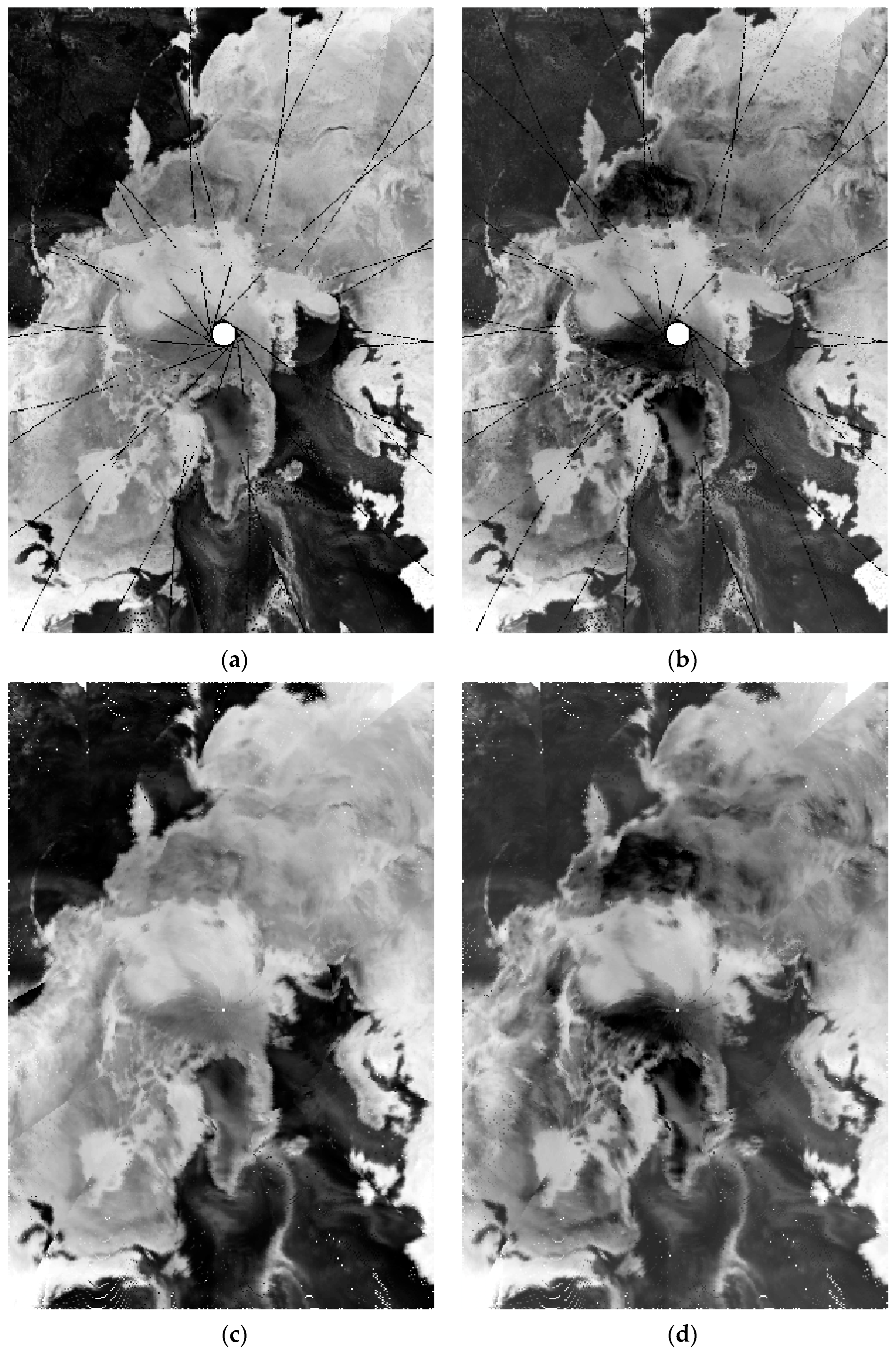
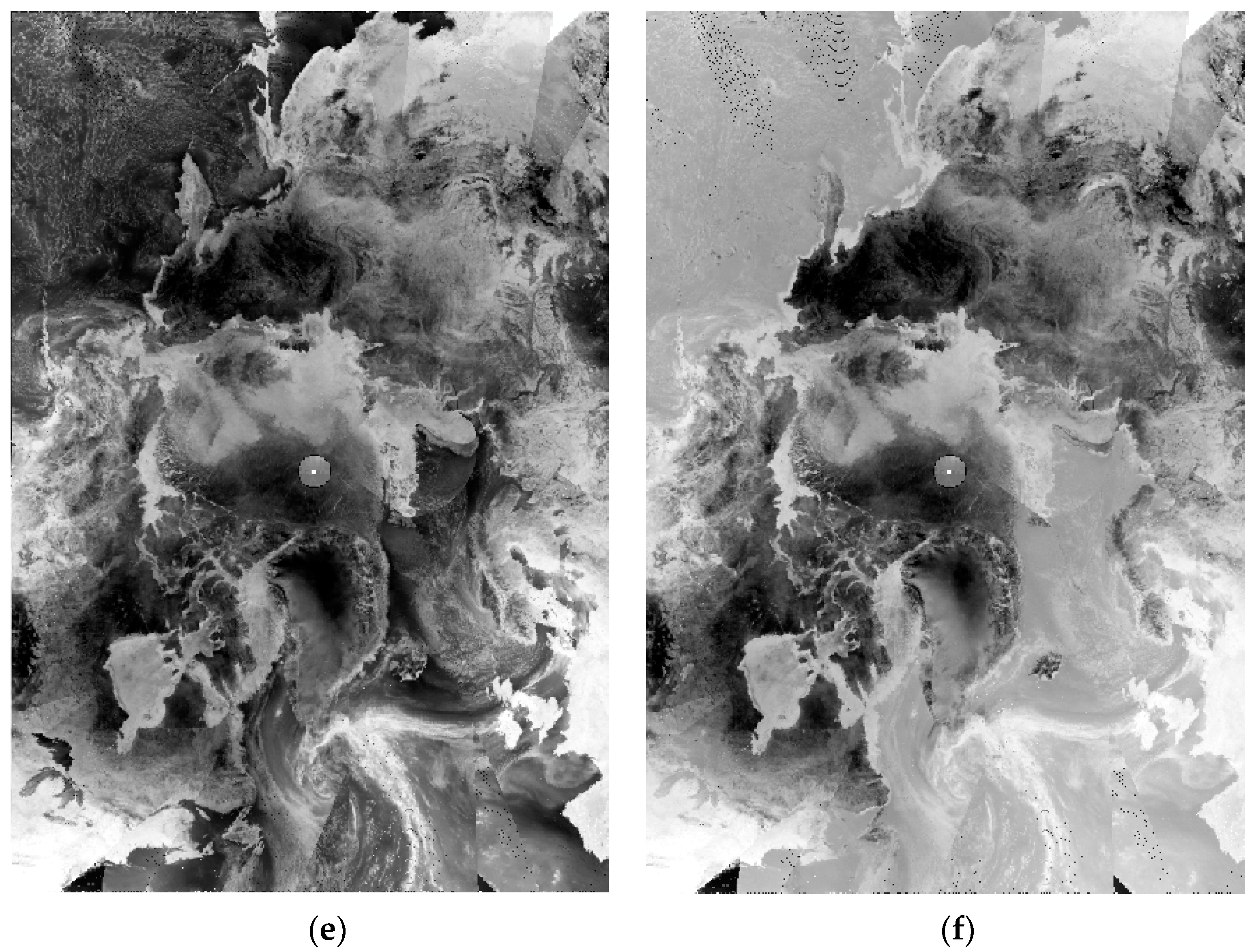
Daily HY-2 and FY-3 data were converted from the WGS84 coordinate system to the polar stereographic projection and extracted brightness temperatures over the Arctic region. Daily brightness temperature data were merged, and the 37 GHz data were gridded into a 25 × 25 km grid and the 89 GHz data into a 12.5 × 12.5 km grid. Neighborhood filtering was used to identify outliers and impute missing values. Figure 2 is an example of the final results. It shows gridded horizontally and vertically polarized brightness temperature data from FY-3 and HY-2 on 1 January 2019, with a resolution of 25 km.
3.2. Retrieval of Sea Ice Drift
To obtain a sea ice drift product with a resolution of 25 km, the brightness temperature data were filtered to remove noise, and a sea ice concentration product was used to exclude areas with concentrations below 15%. We used CMCC to calculate sea ice drift and improved the accuracy of the ice drift vector by replacing outliers (quality control) and using the average value of the retrievals from horizontally and vertically polarized data (polarization fusion).
3.2.1. Gauss Laplace Filter
To reduce data noise and improve data reliability, Laplacian of Gaussian (LOG) filtering [36] was applied to the Arctic brightness temperature data from the four satellites. The Gaussian filtering method involves scanning each pixel in the image with a specified slide window. The weighted average gray value of the pixels in the neighborhood determined by the window was used to replace the value of the pixel point at the center of the window. As that the sliding window used in the CMCC method was 11 × 11 pixels, we also selected 11 × 11 pixels for Gaussian filtering in this paper.
3.2.2. Making a Mask
The 25-km gridded sea ice concentration product from the National Snow and Ice Data Center (NSIDC) for January–April 2019 was used to exclude the areas with sea ice concentrations below 15%. The change in the sea ice concentration between two satellite images with short time intervals (below 14 days) was generally considered to be small. Therefore, the ice concentration of the first image was used to create the sea ice mask.
3.2.3. Continuous Maximum Cross-Correlation Matching
With a search interval of 1 pixel, sea ice drift below 1 pixel cannot be retrieved using MCC [24,25,26]. Therefore, we used CMCC [27,28] to retrieve Arctic sea ice drift. The CMCC is based on MCC; high-resolution (2.5 × 2.5 km) data are obtained by bilinear interpolation of radiometer data and are used for sea ice displacement matching and high-accuracy ice drift retrievals.
In MCC, the sea ice drift displacement vector is evaluated by calculating the correlation coefficient of a set of brightness temperature images on day N and day N + I and selecting the maximum correlation coefficient; N represents the start date of sea ice drift retrieval and I represents the time interval. The correlation coefficient of two images of size M × N is defined as follows:
where u(x,y) is the brightness temperature value of the first image; v(x,y) is the brightness temperature value of the second image; ∘ is the correlation operation; * is the complex conjugation.
For the center of an 11 × 11 pixel slide window of day N, CMCC uses MCC to find the best matching pixel (m,n) in the image of day N + I, and uses bilinear interpolation to generate an image with higher pixel resolution. We used intervals of 0.2 pixels for search and control; therefore, a 5 × 5 pixel window was used for interpolation for each pixel to generate a new image with a resolution of 2.5 × 2.5 km; the new image was used for MCC processing to retrieve the best matching locations to calculate sea ice drift. The slide window center of the image of day N, the location information of the matching locations on day N + I, and the interval (I days) were used to obtain the sea ice drift speed as follows:
where and are sea ice drift speeds in cm/s in the V and U directions, respectively; and are sea ice displacements in the V and U directions, respectively; res is the spatial resolution of the brightness temperature data.
3.2.4. Quality Control
Some of the sea ice drift speed vectors derived using CMCC are inconsistent with the overall drift trend. There are two reasons for drift vector errors: the drift vector falls into the local optimum during the process of maximum correlation, or pixel noise and spatial structure are of the same orders of magnitude or are beyond the range. Therefore, to improve retrieval accuracy, neighborhood filtering was used and drift vectors with large deviations were corrected. Neighborhood filtering was applied to identify outlier vectors, and outlier speed was replaced with the maximum correlation coefficient or the average speed. For each area, the mean and standard deviation of sea ice speed were calculated in the pixels, and pixels with speeds that exceeded the mean by more than twice the standard deviation were excluded.
3.2.5. Polarization Fusion
The radiometer tracks the location of sea ice based on changes in bright temperature. Since the information obtained from the horizontal and vertical polarization data are uncorrelated, fusing the two involves using more information to track the change in the sea ice position [37]. In this paper, we retrieved sea ice drift speeds from horizontally and vertically polarized bright temperature data and used the average value as the final sea ice drift. As a result, the accuracy and reliability of the velocity field improved.
3.3. Evaluation Indicators
The root mean square error (RMSE) and relative error (RE) between the satellite product and buoy data were calculated and used to evaluate the accuracy of the product. The RMSEs and REs of the ice drift speed and direction were calculated as follows:
where and are the drift speeds retrieved from satellite and buoy data, respectively; and are the drift directions retrieved from satellite and buoy data, respectively; n is the number of data points used for the evaluation.
4. Results
4.1. Accuracy of Satellite Products
4.1.1. Effect of Time Interval on the Accuracy of Sea Ice Drift Retrievals
CMCC was used to retrieve sea ice drift in N and N + I day image pairs from SSMIS, AMSR2, FY-3, and HY-2 data. For a time interval of 1 day, drift velocities of ≥1.44 cm/s can be retrieved using CMCC by bilinear interpolation from the 12.5 × 12.5 km to 2.5 × 2.5 km grids. The time interval determines the minimum retrievable drift speed. To examine the effect of the time interval on the accuracy of ice drift products, we retrieved the sea ice drift from the 37 and 89 GHz brightness temperature data using time intervals of 3, 6, and 14 days and compared the retrievals with buoy data.
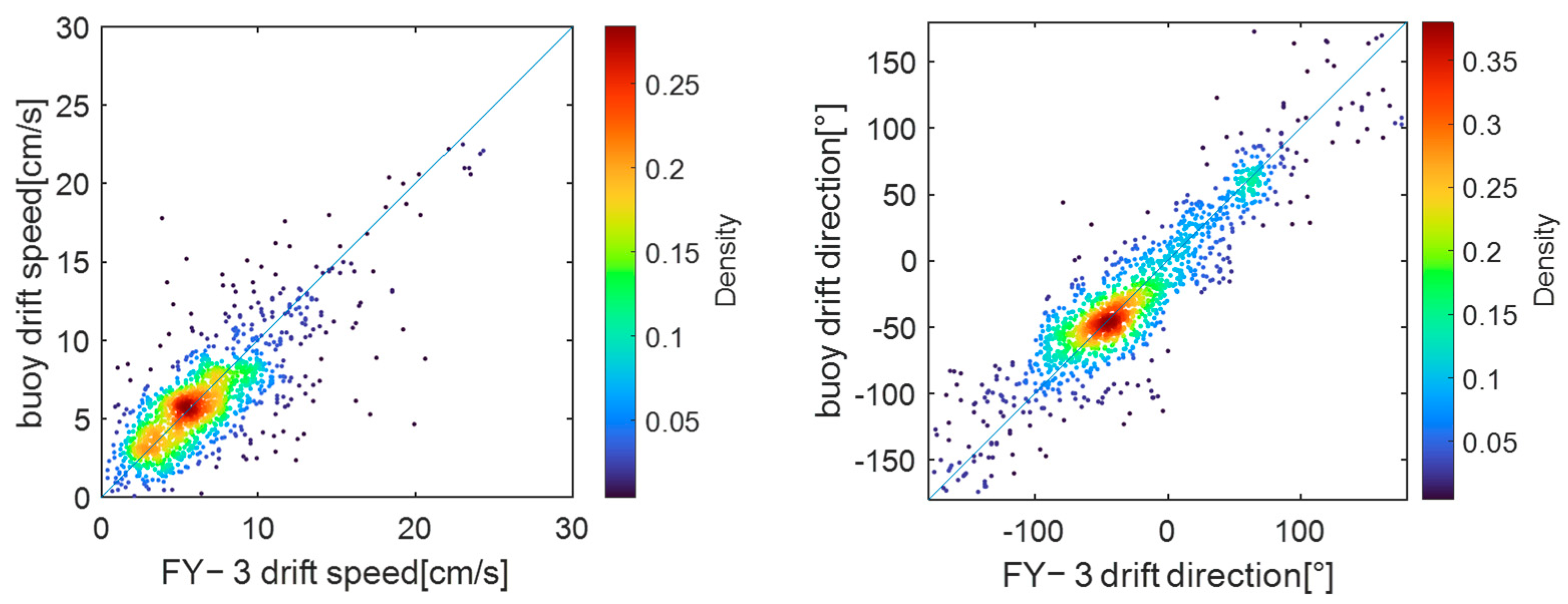
For drift speed and direction retrieved from 37 GHz data for January–April 2019, the RMSEs and REs between the satellite product and IABP buoy data are shown in Table 2 and Table 3; S denotes speed and D denotes direction. The corresponding density scatter plot is shown in Figure 3. For a time interval of 6 days, the RMSEs of SSMIS speed and direction were 0.52 cm/s and 5.56°, respectively, while the RMSEs of AMSR2 speed and direction were 0.51 cm/s and 5.36°, respectively. The REs of the SSMIS speed and direction were 2.37% and 8.50%, respectively, while the REs of the AMSR2 speed and direction were 2.42% and 8.32%, respectively. For a time interval of 14 days, the RMSEs of SSMIS speed and direction were 0.33 cm/s and 4.45°, while the RMSEs of AMSR2 speed and direction were 0.32 cm/s and 4.48°. The REs of SSMIS speed and direction were 2.28% and 9.14%, while the REs of the AMSR2 speed and direction were 2.22% and 7.27%. For intervals of 6 and 14 days, the accuracy of SSMIS products was close to that of AMSR2 products. However, at an interval of 3 days, the RMSEs of SSMIS speed and direction were 0.92 cm/s and 6.83°, and the RMSEs of AMSR2 speed and direction were 0.73 cm/s and 6.49°. The REs of SSMIS speed and direction were 4.00% and 10.83%, and the REs of the AMSR2 speed and direction were 3.70% and 5.30%. The accuracy of SSMIS products was considerably lower than that of AMSR2 products; this may be because the higher raw resolution of AMSR2 data supports the retrieval of ice drift vectors at low speeds.
As can be seen from Figure 3, the drift speeds of the four products are generally concentrated in the range of 0–10 cm/s, and the drift directions are generally concentrated from −90° to 0°. The SSMIS and AMSR2 products are relatively close to the buoy data in terms of speed and direction. The overall speed of the FY-3 product is overestimated, but not much different in terms of direction. Relatively, the RE of the FY-3 product is higher than that of the SSMIS and AMSR2 products in terms of speed. It can be seen that the RE in the speed of the FY-3 product is nearly 2% higher than that of the other two products at an interval of 6 days, and nearly 1% higher in terms of direction. The HY-2 product has a tendency to be overestimated in some areas, resulting in a higher RMSE and RE.
For the same frequency, product accuracy was the highest at the 14-day interval and the lowest at the 3-day interval (Table 2 and Table 3). This may be related to the influence of image noise on retrieved drift speed. Low drift velocities cannot be retrieved using short time intervals because of the low spatial resolution of the radiometer; the effect of the image noise on the retrieved drift speed decreases as the time interval increases. Therefore, longer intervals are associated with higher product accuracy. Because the RMSEs of the SSMIS and AMSR2 products were the highest at an interval of 3 days and the lowest at an interval of 14 days, we conclude that a 3-day interval is insufficient to retrieve ice drift vectors with high accuracy from radiometer data with low spatial resolution while ice drift vectors that are of high accuracy but of low temporal resolution can be retrieved using a 14-day interval. Considering the effect of spatial and temporal resolution of the radiometer, the option of an interval of 6 days is a compromise compared to the ice drift results of a 3-day interval and a 14-day interval.
For a time interval of 6 days, the RMSEs of FY-3 speed and direction were 0.77 cm/s and 6.49°, respectively, while the RMSEs of HY-2 speed and direction were 1.40 cm/s and 7.31°, respectively. The accuracy of HY-2 and FY-3 ice drift products was lower than that of SSMIS and AMSR2 products; this is related to the relatively large number of outliers in HY-2 and FY-3 data. For example, on 1 March 2019, outliers accounted for 0.67% (or 3644 data points) of the gridded FY-3 brightness temperature data and 20.39% (or 111,052 data points) of the gridded HY-2 brightness temperature data. There were fewer outliers in FY-3 than in HY-2 data. After interpolation, the FY-3 product was only 0.25 cm/s higher than the SSMIS product at the 6-day interval.
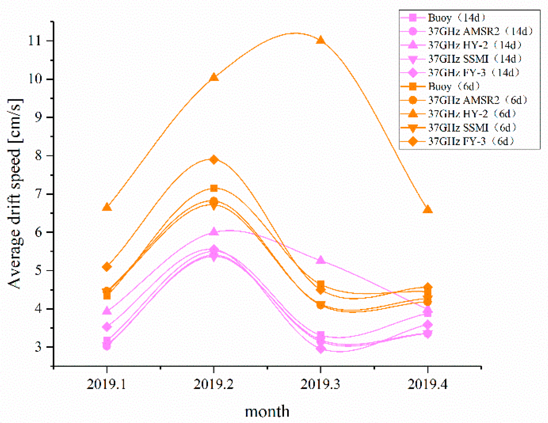
Figure 4 shows the monthly average drift speeds retrieved from buoy data and four sets of satellite data with intervals of 6 and 14 days for January–April 2019. Average monthly ice drift speed decreased with increasing time intervals. By increasing the time interval from 6 to 14 days, the average speed retrieved from buoy data was reduced by 22%, the average speed retrieved from AMSR2 and SSMIS data was reduced by 23%, the average speeds retrieved from FY-3 and HY-2 data were reduced by 29% and 44%, respectively. Retrievals of sea ice displacement do not reflect the actual distances traveled by ice floes; they measure the relative distances that have been covered by floes over a certain period of time. For example, for an ice floe that moves in a circle and is in the same location at the moment of acquisition of the first and a subsequent image, the retrieved displacement and velocity are zero, while the actual displacement and velocity are non-zero. Therefore, the retrieved velocity is lower than the instantaneous velocity of the ice floe at the moment of image acquisition, and higher retrieved velocities are associated with shorter time intervals [32].
Relative to the monthly average drift speed retrieved from buoy data at an interval of 14 days, the average speeds retrieved from AMSR2 and SSMIS were lower by 5%, the average speed retrieved from FY-3 was lower by 1%, and that retrieved from HY-2 was higher by 17%. Relative to the monthly average drift speed retrieved from buoy data at an interval of 6 days, the average speeds retrieved from the AMSR2 and SSMIS products were lower by 4%, while those retrieved from FY-3 and the HY-2 products were higher by 6% and 46%, respectively. Retrieved drift velocities were lower than actual velocities because of the low spatial resolution of the radiometers. Drift velocities retrieved from HY-2 were considerably higher than those from buoy data, and velocities retrieved from FY-3 were slightly higher than those retrieved from the other satellites. This is because of the outliers in FY-3 bright temperature data, which varied in number and location with time. For example, for March 2019, the average drift velocity retrieved from HY-2 was 57% higher than that retrieved from buoy data; outliers accounted for 40% of the corresponding HY-2 brightness temperature data on days 2 and 3, and accounted for more than 30% of the brightness temperature data on days 17, 20, and 21.
4.1.2. Effect of Frequency on the Accuracy of Sea Ice Drift Retrievals
Table 4, Table 5 and Table 6 show the RMSEs of the drift speed and direction retrieved from 37 and 89 GHz SSMIS, AMSR2, and FY-3 data at intervals of 3 days, 6 days, and 14 days for January–April 2019. The corresponding REs are shown in Table 7, Table 8 and Table 9. Retrievals from HY-2 were excluded from the analysis because 89 GHz data were not available from this satellite. Figure 5 shows the density scatter plot of sea ice drift and direction retrieved from buoy data and 89 GHz SSMIS, AMSR2, and FY-3 data at an interval of 6 days for January–April 2019.
For FY-3, accuracy was higher at 89 GHz than at 37 GHz. For SSMIS and AMSR2, accuracy was slightly lower at 89 GHz than at 37 GHz; the difference was generally no more than 0.04 cm/s. However, at an interval of 3 days, the AMSR2 speed error at 89 GHz was higher than that at 37 GHz by 0.36 cm/s. For SSMIS and AMSR2, errors at 89 GHz were higher than those at 37 GHz; this may be caused by the influence of water vapor on the high-frequency channel of the SSMIS and AMSR2 radiometers [38]. The low accuracy of the 37 GHz FY-3 product was probably related to outliers in the brightness temperature data between orbits (Figure 2a,b), while there were no outliers in the 89 GHz FY-3 data (Figure 2e,f). The outliers may have been caused by an abnormality during the image acquisition at 37 GHz in the FY-3 sensor. Proximity interpolation was used to replace outlier values. At a low frequency, the accuracy of SSMIS and AMSR2 products was generally higher than that of the FY-3 product; at a high frequency, the accuracy of the FY-3 product was higher than that of SSMIS and AMSR2 products. A similar tendency is reflected in the REs. However, there are higher REs in some cases. For example, the RE in the speed for these products with a 3-day interval is higher than the 17% in March to April. From Table 7, Table 8 and Table 9, we find that when the RE in the speed is small, the RE in the direction is larger and vice versa. When the time interval increases, the RE of the products in the speed decreases, and the RE of the direction increases.
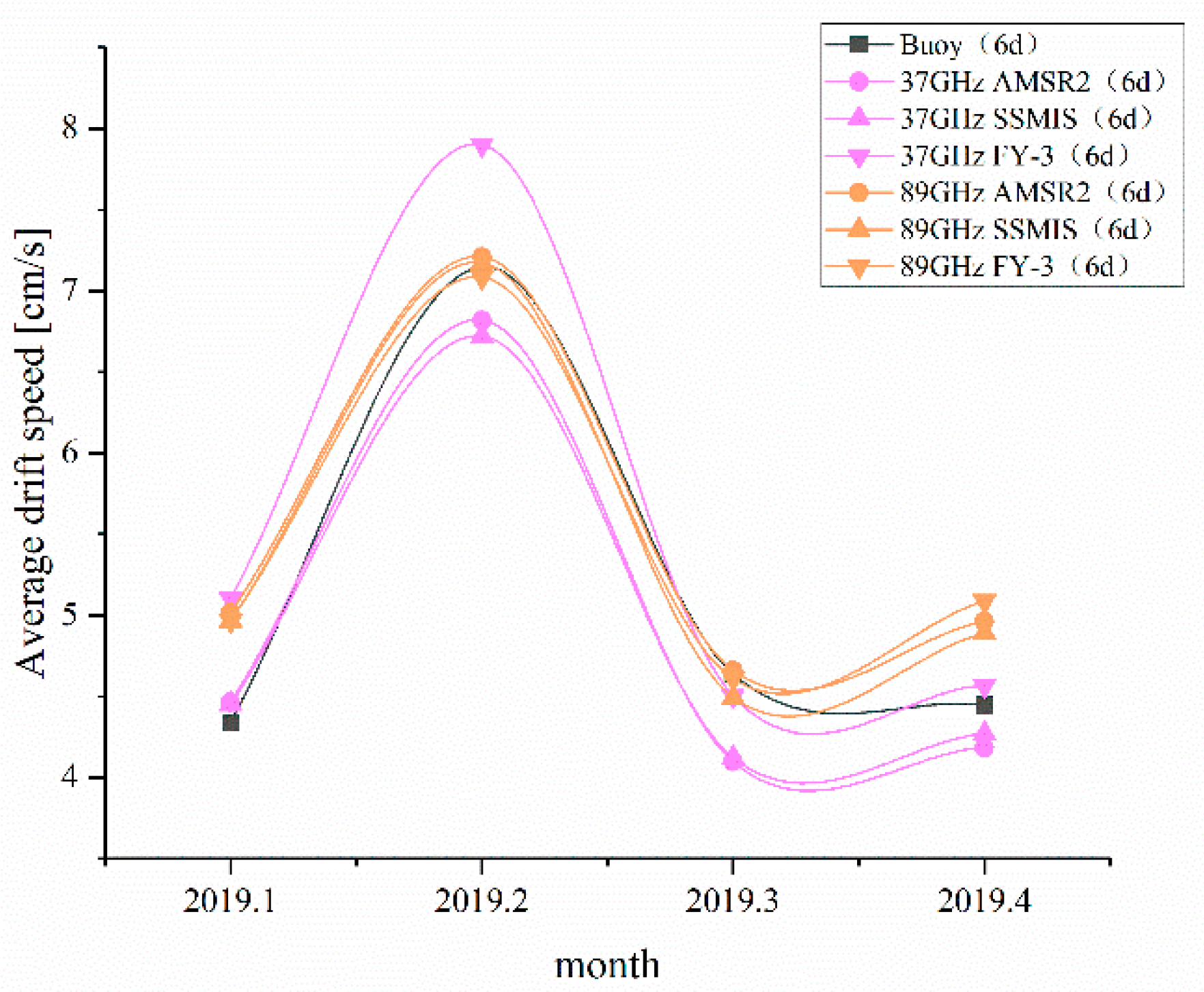
Figure 6 shows average monthly drift speeds retrieved from buoy data and 37 and 89 GHz AMSR2, SSMIS, and FY-3 data at an interval of 6 days. For SSMIS and AMSR2, monthly average drift speeds retrieved from 89 GHz data were higher than those retrieved from 37 GHz data (Table 5). This is because low velocities cannot be retrieved from brightness temperature data with a low spatial resolution; therefore, drift speeds retrieved from low-resolution data are slightly lower than those from high-resolution data. At 89 GHz, the average monthly speed from FY-3 was close to that from SSMIS and AMSR2; at 37 GHz, the average monthly speed from FY-3 was higher than that from SSMIS and AMSR2 by 11%. Therefore, we conclude that the accuracy of FY-3 products is higher at 89 GHz than at 37 GHz.
4.1.3. Drift Speed Error Distribution
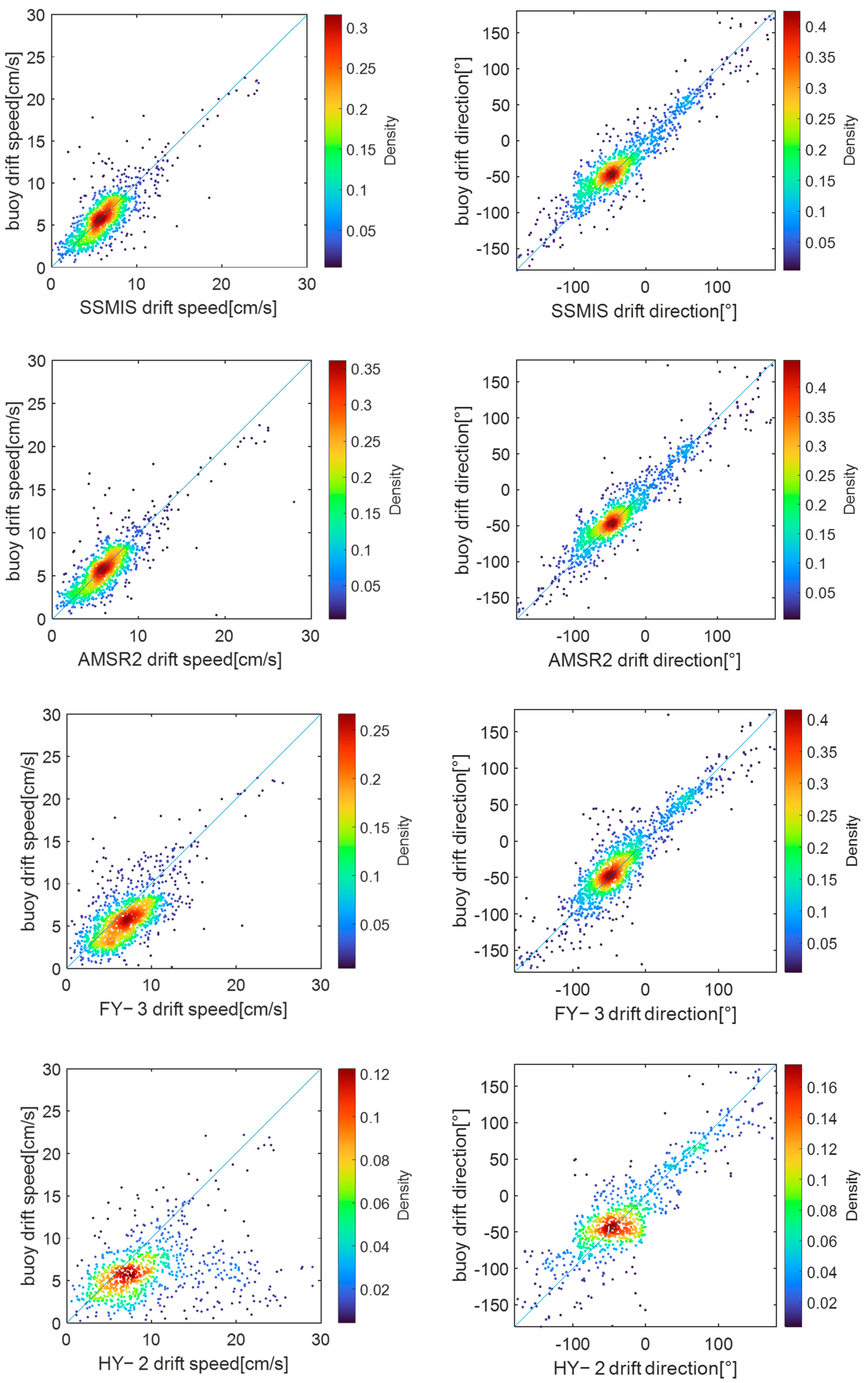
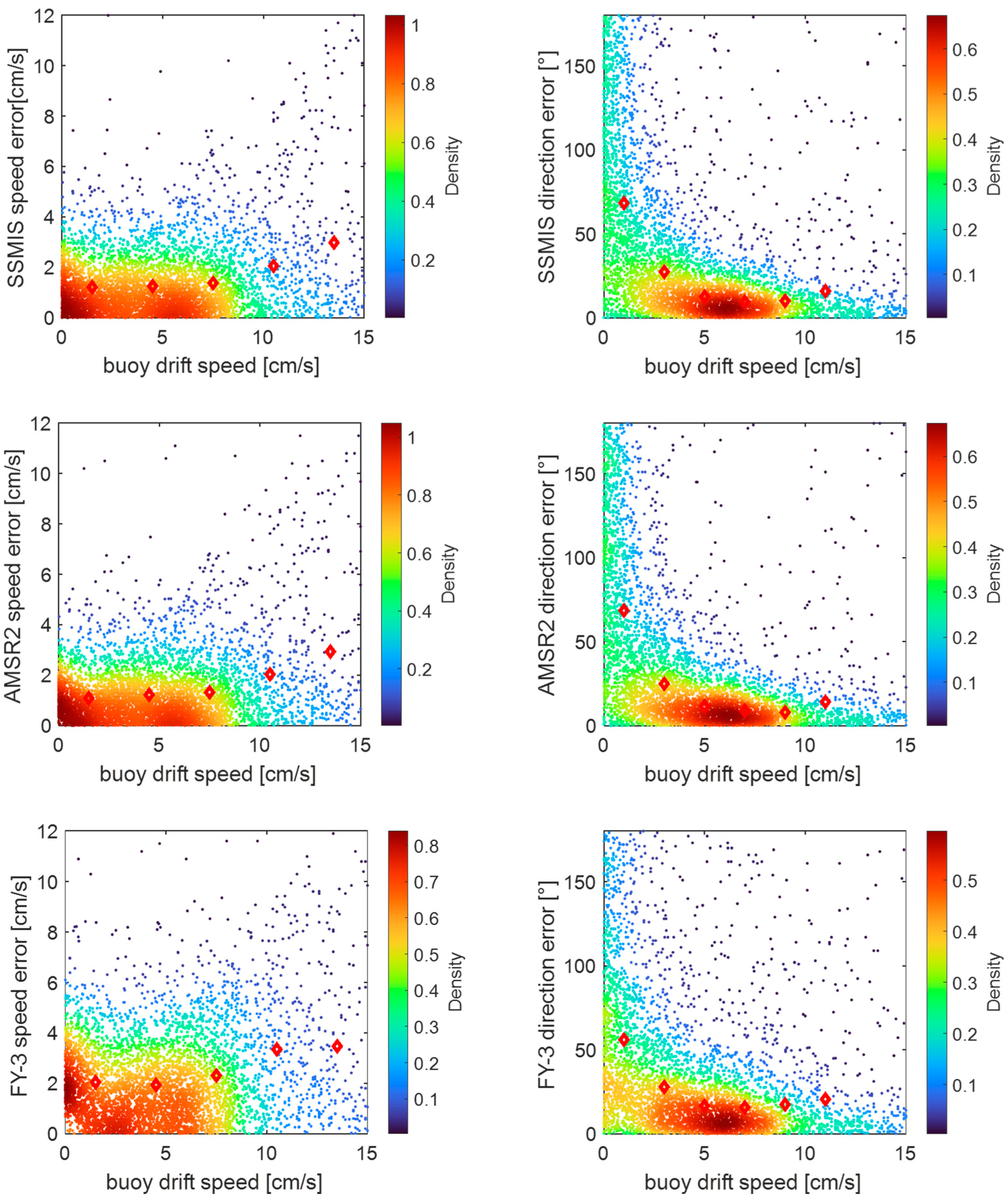
The relationships between retrieved ice drift speed, drift speed error, and drift direction error vary according to the satellite product. Therefore, we examined these relationships by using three sea ice drift products at 89 GHz. A 6-day interval was used for the analysis because of the optimal accuracy and temporal resolution (Section 4.1.1). Figure 7 shows the density scatter plot of sea ice drift speed retrieved from buoy data and the differences between buoy and satellite retrievals of sea ice speed and direction at an interval of 6 days. The red diamonds indicate differences averaged over intervals of 3 or 2 cm/s in buoy drift speed.
For all products, speed error was positively correlated with buoy drift speed, and errors increased with speed. The speed error of the AMSR2 product was considerably lower than that of the other two products, especially at low speeds. The overall speed error of the AMSR2 product was the smallest. This indicates that the AMSR2 product is superior in tracking sea ice at low speeds. The speed error of the FY-3 product was higher than that of the SSMIS product by about 1 cm/s. Errors in retrieved sea ice drift direction were particularly large at very low speeds; they decreased gradually with increasing speed.
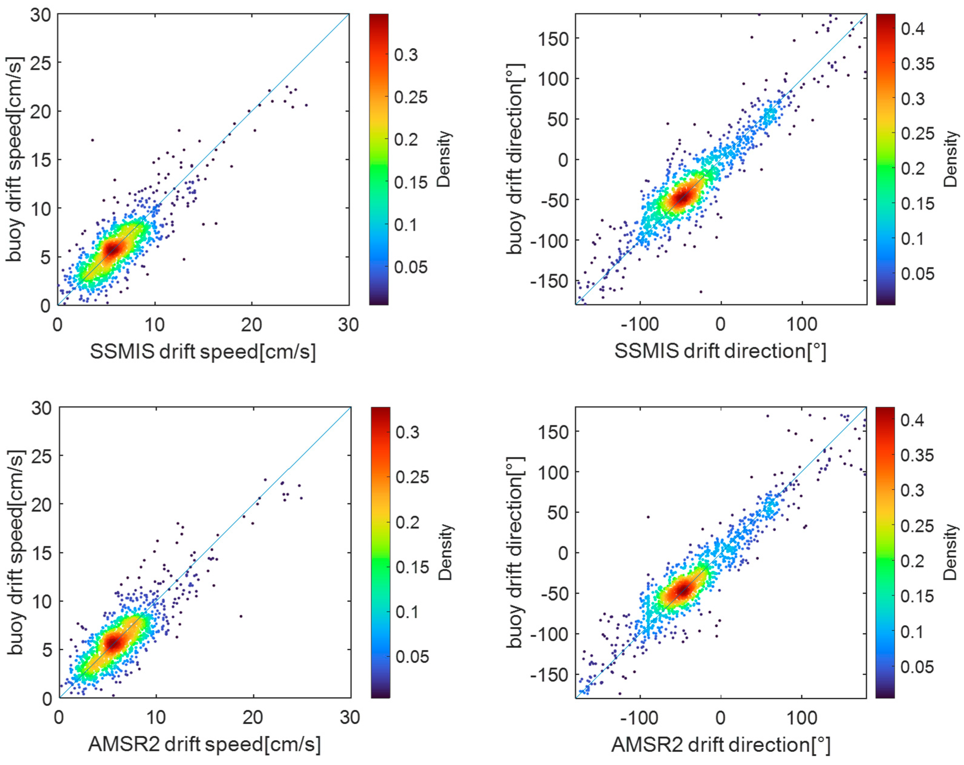
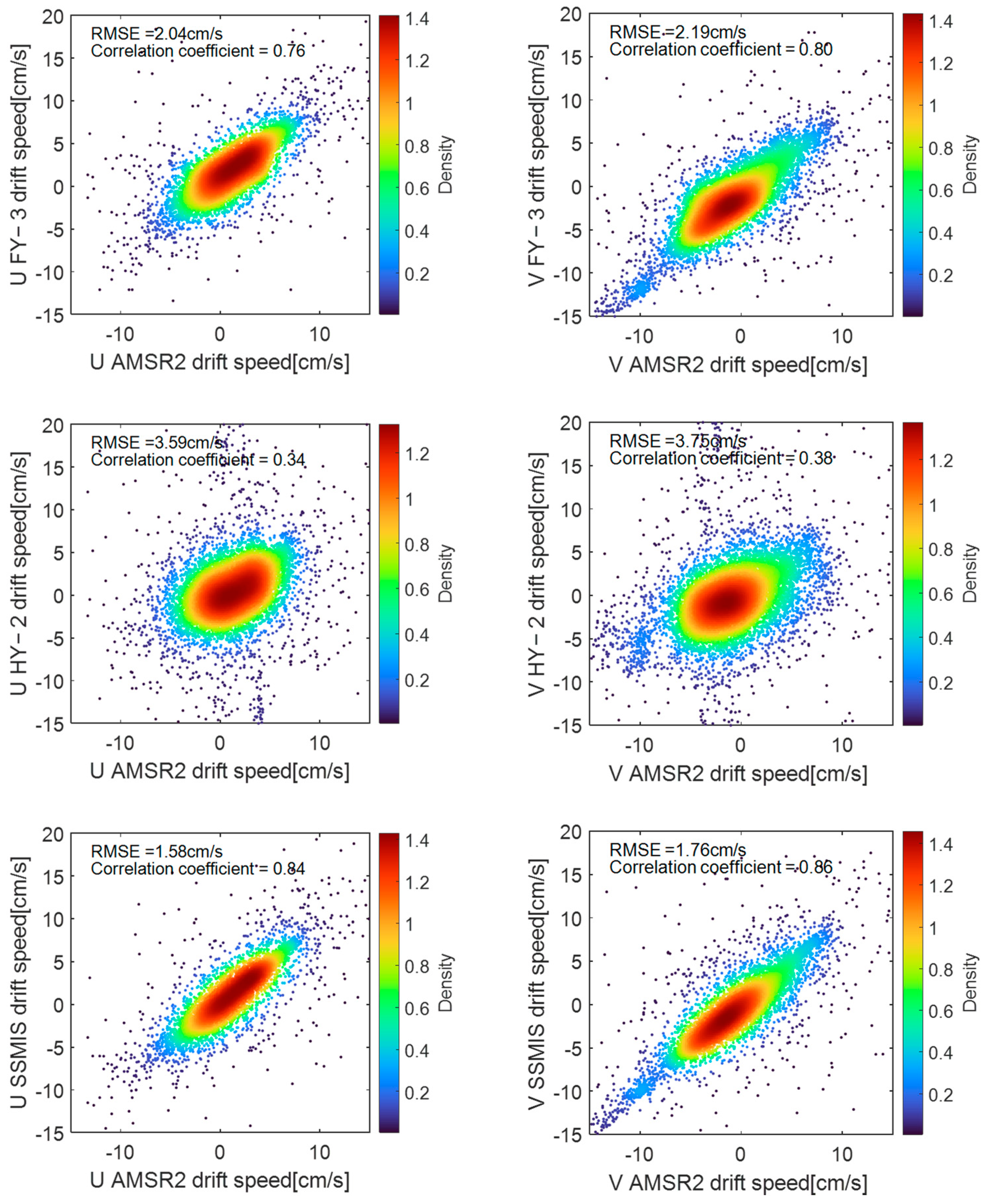
4.2. Correlation between Retrieved Drift Speeds
Given that all four ice drift products adopted the sea ice drift results in U and V directions, Figure 8 shows the density scatter plots of sea ice drift speeds in the U and V directions retrieved from 37 GHz FY-3, HY-2, AMSR2, and SSMIS data for January–April 2019. The correlation coefficients between FY-3 and AMSR2, between FY-3 and SSMIS, and between SSMIS and AMSR2 were high. The correlation coefficients between SSMIS and AMSR2 were the highest; for the U and V directions, correlation coefficients were 0.84 and 0.86, respectively, and RMSEs were 1.58 and 1.76 cm/s, respectively. The correlation coefficients between AMSR2 and FY-3 were the second highest; for the U and V directions, correlation coefficients were 0.76 and 0.80, and RMSEs were 2.04 and 2.19 cm/s. For the U and V directions, the correlation coefficients between FY-3 and SSMIS were 0.76 and 0.78, and RMSEs were 2.03 and 2.28 cm/s. The correlation coefficients between HY-2 and the other three products were low; they were around 0.4, with RMSEs of approximately 3.0 cm/s.
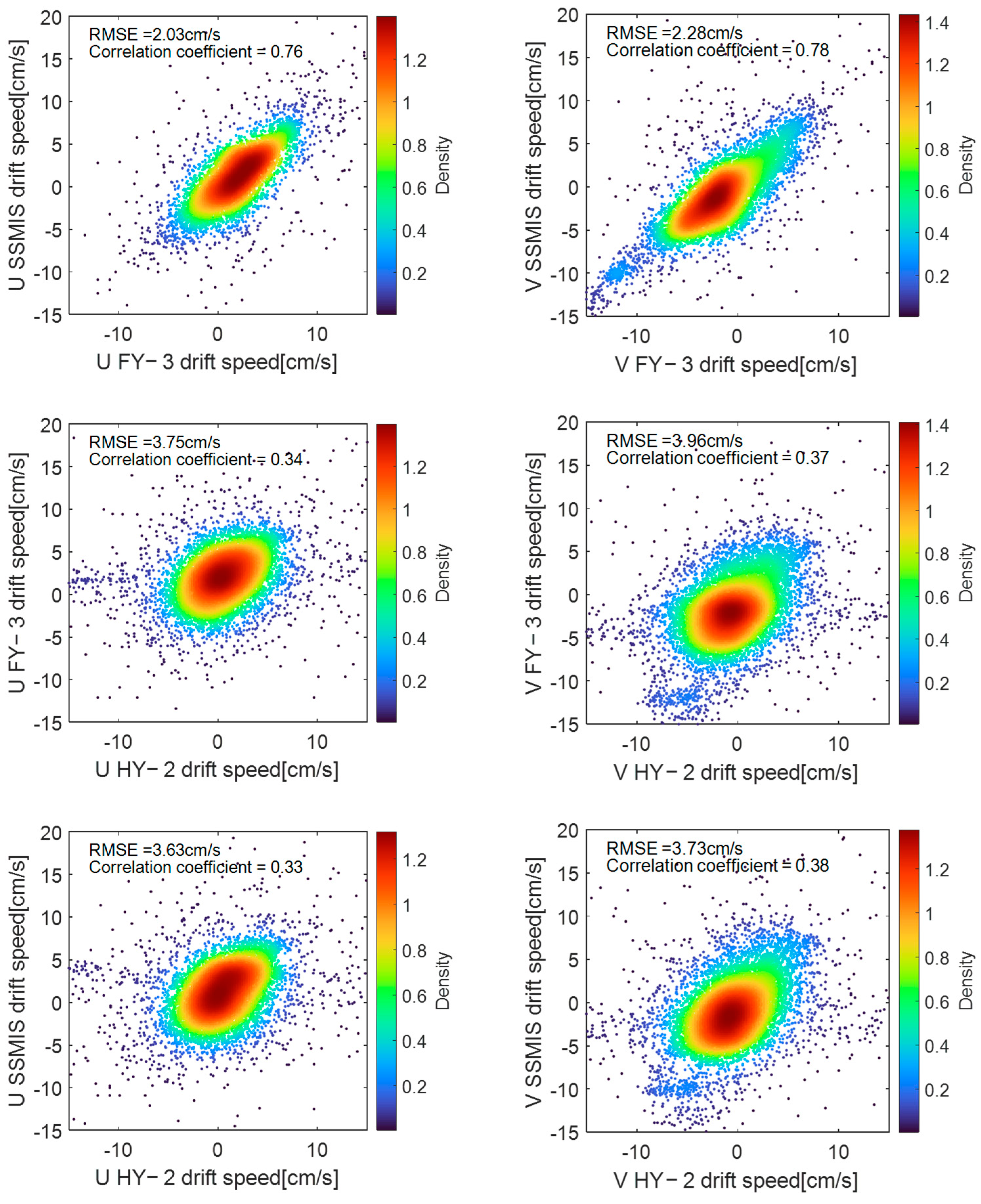
Figure 9 is a density scatter plot of sea ice drift speeds in the U and V directions retrieved from 89 GHz FY-3, AMSR2, and SSMIS data for January–April 2019. The correlation coefficients between AMSR2 and FY-3 were the highest. For the U and V directions, correlation coefficients were 0.74 and 0.84, respectively, and RMSEs were 1.78 and 1.86 cm/s, respectively. For the U and V directions, correlation coefficients between SSMIS and AMSR2 were 0.69 and 0.80, and RMSEs were 2.20 and 2.18 cm/s. For the U and V directions, correlation coefficients between FY-3 and SSMIS were 0.58 and 0.74, and RMSEs were 2.46 and 2.45 cm/s. Correlation coefficients were slightly lower at 89 GHz than at 37 GHz; this may be related to the influence of water vapor on the 89 GHz radiometer data.
Retrieved sea ice drift speeds were generally low and between +15 and −15 cm/s. There were large differences between the retrieved speeds at the pixel levels at some grid points. The outliers in HY-2 led to extremely large deviations in the values of the maximum correlated image element; large deviations at low drift speeds resulted in a low correlation between HY-2 and the other products. Overall, the correlation between FY-3 and AMSR and that between FY-3 and SSMIS were high. In the density scatter plots between FY-3 and AMSR2 and between FY-3 and SSMIS, the data scatter was highly concentrated; only a small proportion of the scatter was associated with grid points with large differences between FY-3 and AMSR2 speeds or between FY-3 and SSMIS speeds (Figure 9).
5. Discussion
The spatial distribution of retrieved ice drift speed varies according to the satellite product and may be related to the sea ice concentration. Figure 10a shows the sea ice concentration over the Arctic basin. We explored the impact of sea ice concentration on the differences between drift ice speeds retrieved from four sets of satellite data for January–April 2019. We used AMSR2 as the basis for the density scatter plots in Figure 10b–d. To improve the accuracy of the products, grid points with sea ice concentrations of less than 15% were removed during the retrieval of sea ice drift, and data for areas with low ice concentrations are excluded from Figure 10b–d.
The difference between ice speeds was negatively correlated with sea ice concentration; low concentrations were associated with large speed differences. By increasing the concentration from 15% to 80%, the difference between ice drift speed retrieved from SSMIS and that from AMSR2 decreased from 2.04 to 0.56 cm/s; the difference between HY-2 and AMSR2 decreased from 5.81 to 3.72 cm/s. By increasing the concentration from 15% to 70%, the difference between the ice drift speed retrieved from FY-3 and that from AMSR2 decreased from 2.38 to 1.61 cm/s. For all products, speed differences were high at concentrations of 80–90%; at concentrations exceeding 90%, speed differences decreased; presumably, this is because the number of pixels with large speed differences increased at concentrations exceeding 80%. The differences between drift speeds retrieved from SSMIS and those from AMSR2 were the smallest. The differences between drift speeds retrieved from FY-3 and those from AMSR2 remained small for concentrations below 70%; at concentrations of 70–90%, differences were relatively large. The differences between drift speeds retrieved from HY-2 and those from AMSR2 were large; this is consistent with the effects of the large outliers at low drift speeds that are discussed in Section 4.2.
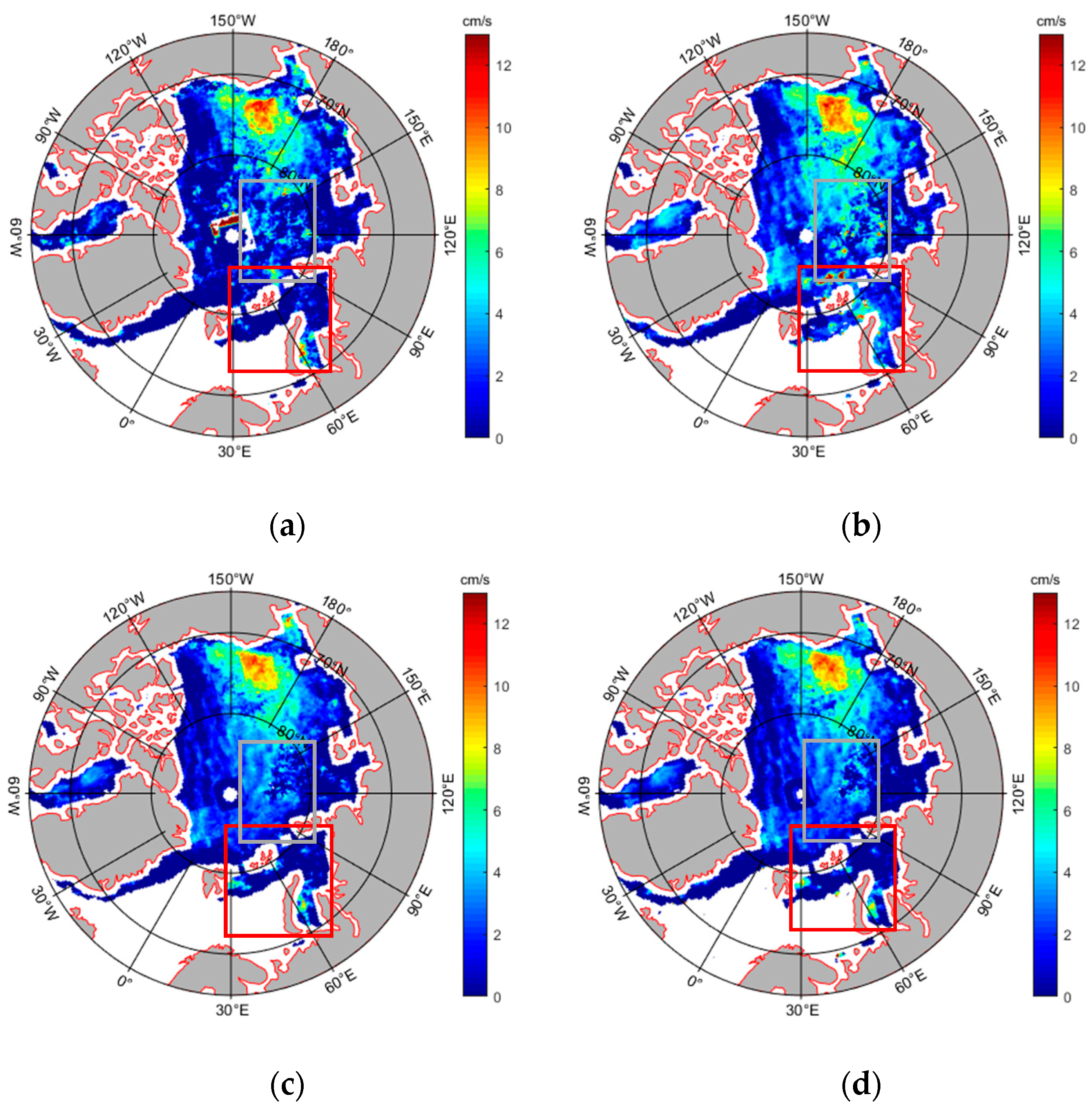
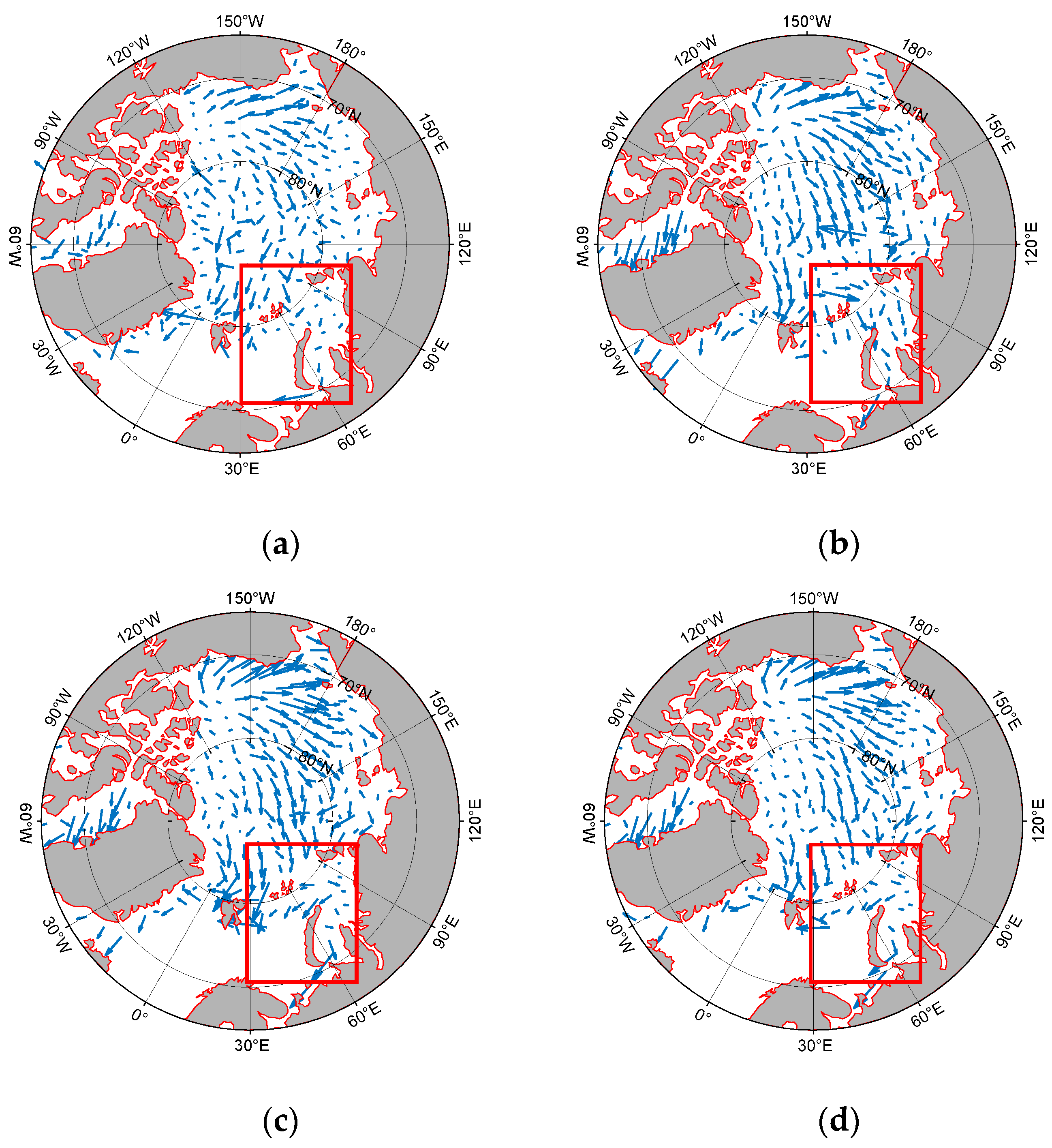
We explored the effect of sea ice concentration on the spatial distribution of the retrieved ice drift speed and direction. Figure 11 shows the distribution of the average sea ice drift speed in the Arctic retrieved from HY-2, FY-3, AMSR2, and SSMIS data for January 2019; gray shading indicates the land area and the thin red line represents the coastline. Figure 12 shows the sea ice drift direction retrieved from HY-2, FY-3, AMSR2, and SSMIS data for January 2019; blue arrows indicate sea ice drift velocity.
All retrieved Arctic sea ice drifts were anticyclonic (Figure 12). The four products shared similar characteristics, such as high drift velocities in northern Alaska, where the monthly average drift speed reached 13 cm/s; ice drifted from the north of Cape Barrow to northern Russia; speeds were extremely low and were close to 0 cm/s in the northern Canadian Archipelago; in the central Arctic, drift directions were between 150°W and 30°E. In the gray rectangle in Figure 11, the speeds retrieved from AMSR2 were close to those retrieved from SSMIS; the speeds retrieved from HY-2 and FY-3 were higher and were associated with large drift vectors; ice concentration was 70–90% and errors in the speeds retrieved from FY-3 were large (Figure 10b). There were spatial differences between the four ice drift products; the largest speed and direction differences were concentrated in the marginal ice zone and between eastern Iceland and western Russia (red rectangles in Figure 11 and Figure 12).
Differences between retrieved drift speeds (Figure 11) were mainly related to sea ice concentration (Figure 10a); differences were large at low concentrations and small at high concentrations. There is more variability in satellite retrievals of sea ice motion during the early stages of freezing and melting because of the enhanced atmospheric influence on the satellite signal and the rapid changes in sea ice surface emissivity. Therefore, the variabilities in sea ice drift retrievals were higher and differences between speed retrievals were larger at low ice concentrations [33]. For some regions, drift speeds retrieved from FY-3 and HY-2 data were higher than those retrieved from SSMIS and AMSR2; for other regions, the speeds retrieved from the different datasets were comparable.
6. Conclusions
In this study, CMCC was used to generate sea ice drift products from China’s FY-3 and HY-2 radiometer data, and FY-3 and HY-2 products were compared with sea ice drift products retrieved from AMSR2 and SSMIS radiometer data. Product accuracy was evaluated using IABP buoy data. In addition, we examined the correlation between products and analyzed the factors underlying errors in the retrievals. Our main conclusions are as follows:
- High-accuracy ice drift products can be obtained from FY-3 and HY-2 radiometer bright temperature data. Comparing ice drift vectors retrieved from IABP buoy data and 37 GHz satellite data in a 6-day time interval, we found that the errors in the FY-3 (RMSEs in the drift speed and direction relative to buoy data: 0.77 cm/s and 6.49°; REs in the drift speed and direction relative to buoy data: 4.38% and 9.23%) and HY-2 (RMSEs in the drift speed and direction: 1.40 cm/s and 7.31°; REs in the drift speed and direction: 5.78% and 6.44%) products were slightly higher than those in the SSMIS (RMSEs in the drift speed and direction: 0.52 cm/s and 5.56°; REs in the drift speed and direction: 2.37% and 8.50%) and AMSR2 (RMSEs in the drift speed and direction: 0.51 cm/s and 5.36°; REs in the drift speed and direction: 2.42% and 8.32%) products. In general, the accuracies of the HY-2 and FY-3 products were slightly lower than those of the SSMIS and AMSR2 products, but the differences were small and met the international requirements for ice drift products.
- There is a close agreement between the sea ice drift vectors retrieved from the four sets of satellite data. Between the FY-3, SSMIS, and AMSR2 products, correlation coefficients and RMSEs were higher at 37 GHz (correlation coefficients: 0.76–0.86; RMSEs: 1.58–2.28 cm/s) than at 89 GHz (correlation coefficients: 0.58–0.84; RMSEs: 1.78–2.46 cm/s). In general, the correlation between FY-3, SSMIS, and AMSR2 products was high, while the correlation between HY-2 and the other products was low. Discrete point values in regions of low drift speeds impacted retrieval results.
- There was consistency between the spatial distributions of drift speeds retrieved from the four sets of radiometer data. Differences between products were negatively correlated with sea ice concentrations; large differences were associated with low sea ice concentrations. The retrieved sea ice drift speed was high in northern Alaska and extremely low in the northern Canadian Archipelago. There were spatial differences in the speed and direction of the different products; the largest differences were concentrated at the ice edge and between eastern Iceland and western Russia; this reflects the influence of the sea ice concentration on the spatial distribution of ice drift. Differences in the drift speeds were large in areas with low ice concentrations and small in areas with high ice concentrations. Retrievals of sea ice drift can be used in the formulation of local marine protection measures.
In conclusion, differences in radiometer frequency and spatial and temporal resolutions result in differences in sea ice drift products. In this study, we compared and evaluated different ice drift products for January–April 2019. During this period, there were many outliers in the HY-2 data, and the accuracies of the sea ice drift vectors retrieved from HY-2 data were low. However, the retrieval accuracy will improve with the improvement of the HY-2 satellite data.
Author Contributions
X.Z. proposed the idea. H.F. and X.Z. simulated the experiment. H.F., X.Z. and M.B. analyzed the results and wrote the text. L.S., J.Z., G.L. and C.C. supervised the work. All authors have read and agreed to the published version of the manuscript.
Funding
This research was funded in part by the National Key Research and Development Program of China under grant 2021YFC2803300; in part by the National Natural Science Foundation of China under grants 41976173 and 61971455; the Shandong joint fund of National Natural Science Foundation of China under grant U2106211; the Shandong Provincial Natural Science Foundation, China under grant ZR2019MD016; and the Ministry of Science and Technology of China and the European Space Agency through the Dragon-5 Program under grant 577889.
Acknowledgments
We would like to thank the NSIDC for providing SSMIS data, AMSR2 data, SIC data and IABP buoy data, the National Satellite Meteorological Center for providing FY-3 data, and the National Satellite Ocean Application Service for providing HY-2 data.
Conflicts of Interest
The authors declare no conflict of interest.
References
- Liu, M.; Yan, R.; Zhang, J.; Xu, Y.; Chen, P.; Shi, L.; Wang, J.; Zhong, S.; Zhang, X. Arctic Sea Ice Classification Based on CFOSAT SWIM Data at Multiple Small Incidence Angles. Remote Sens. 2022, 14, 91. [Google Scholar] [CrossRef]
- Liu, M.; Dai, Y.; Zhang, J.; Zhang, X.; Meng, J. Analysis of sea-ice condition in the Bohai Sea based on multi-source remote sensing data in the 2009–2010 winter. Dragon 3mid Term Results 2014, 724, 92. [Google Scholar]
- Zhang, F.; Pang, X.; Lei, R.; Zhai, M.; Zhao, X.; Cai, Q. Arctic sea ice motion change and response to atmospheric forcing between 1979 and 2019. Int. J. Climatol. 2022, 42, 1854–1876. [Google Scholar] [CrossRef]
- Spreen, G.; Kwok, R.; Menemenlis, D. Trends in Arctic sea ice drift and role of wind forcing: 1992–2009. Geophys. Res. Lett. 2011, 38, 19. [Google Scholar] [CrossRef] [Green Version]
- Ji, Q. Spatial and Temporal Variation of Arctic Sea Ice Thickness Based on Satellite Altimetry. Ph.D. Thesis, Wuhan University, Wuhan, China, 2015. [Google Scholar]
- Amstrup, S.C.; DeWeaver, E.T.; Douglas, D.; Marcot, B.G.; Durner, G.M.; Bitz, C.; Bailey, D.A. Greenhouse gas mitigation can reduce sea-ice loss and increase polar bear persistence. Nature 2010, 468, 955–958. [Google Scholar] [CrossRef]
- Zhang, L.; Tan, H. Analysis of global sea ice simulation with BCC_CSM model and its error causes. In Proceedings of the 32nd Annual Meeting of Chinese Meteorological Society, Tianjin, China, 14 October 2015; p. 170. [Google Scholar]
- Qiu, B.; Li, C.; Guan, C. Effects of Arctic sea ice drift on multi-year ice distribution. Bull. Oceanol. Limnol. Sin. 2019, 3, 11. [Google Scholar]
- Denis, D.; Vladimir, V.; Eduard, K. Sea Ice Drift Tracking From Sequential SAR Images Using Accelerated-KAZE Features). IEEE Trans. Geosci. Remote Sens. 2017, 55, 5174–5184. [Google Scholar]
- Ye, Y.; Mohammed, S.; Georg, H.; Gunnar, S. Improving Multiyear Sea Ice Concentration Estimates with Sea Ice Drift. Remote Sens. 2016, 8, 397. [Google Scholar] [CrossRef] [Green Version]
- Ron, K. Sea ice concentration estimates from satellite passive microwave radiometry and openings from SAR ice motion. Geophys. Res. Lett. 2002, 29, 9. [Google Scholar]
- Jiménez, C.; Tenerelli, J.; Prigent, C.; Kilic, L.; Lavergne, T.; Skarpalezos, S.; Høyer, J.; Reul, N.; Donlon, C. Ocean and Sea Ice Retrievals From an End-To-End Simulation of the Copernicus Imaging Microwave Radiometer (CIMR) 1.4–36.5 GHz Measurements. J. Geophys. Res. Ocean. 2021, 126, 12. [Google Scholar] [CrossRef]
- Ming, Z.; Junkai, W.; Xiaoqi, L.; Xi, Z.; Jing, L.; Genwang, L.; Ting, Z. Detection of sea ice drift based on different polarization data. Laser Optoelectron. Prog. 2019, 56, 6. [Google Scholar]
- Zhang, M.; An, J.; Zhang, J.; Yu, D.; Wang, J.; Lv, X. Application of Feature Tracking and Pattern Matching Algorithm in Sea ice Drift Detection. Laser Optoelectron. Prog. 2019, 56, 7. [Google Scholar]
- Xu, J.; Zhang, X.; Wang, K. Sea ice drift monitoring method based on bilateral function global motion model. Spacecr. Eng. 2019, 28, 6. [Google Scholar]
- Hong, S.H.; Kim, J.H.; Park, J.W.; Won, J.S. Detection and Speed Measurement of Brash Ice in the Arctic Ocean by TerraSAR-X Quad-pol SAR. J. Coast. Res. 2019, 90, 1. [Google Scholar] [CrossRef]
- Wang, Y. Non-Homologous Sea ice SAR Image Registration Based on Significant Gray Difference; Dalian Maritime University: Dalian, China, 2020. [Google Scholar]
- Zhang, X.; Zhu, Y.; Zhang, J.; Meng, J.; Li, X.; Li, X. An Algorithm for Sea Ice Drift Retrieval Based on Trend of Ice Drift Constraints from Sentinel-1 SAR Data. J. Coast. Res. 2020, 102, 113–126. [Google Scholar] [CrossRef]
- Zhang, M.; An, J.; Zhang, J.; Yu, D.; Wang, J.; Lv, X. Enhanced Delaunay Triangulation Sea Ice Tracking Algorithm with Combining Feature Tracking and Pattern Matching. Remote Sens. 2020, 12, 581. [Google Scholar] [CrossRef] [Green Version]
- Dierking, W.; Stern, H.; Hutchings, J.K. Estimating statistical errors in retrievals of ice speed and deformation parameters from satellite images and buoy arrays. Cryosphere 2020, 14, 2999–3016. [Google Scholar] [CrossRef]
- Shokr, M.E.; Wang, Z.; Liu, T. Sea ice drift and arch evolution in the Robeson Channel using the daily coverage of Sentinel-1 SAR data for the 2016–2017 freezing season. Cryosphere 2020, 14, 3611–3627. [Google Scholar] [CrossRef]
- Barbat, M.M.; Rackow, T.; Wesche, C.; Hellmer, H.H.; Mata, M.M. Automated iceberg tracking with a machine learning approach applied to SAR imagery: A Weddell sea case study. ISPRS J. Photogramm. Remote Sens. 2021, 172, 189–206. [Google Scholar] [CrossRef]
- Xu, L.; Wong, W. A KPCA texture feature model for efficient segmentation of RADARSAT-2 SAR sea ice imagery. Int. J. Remote Sens. 2014, 35, 5053–5072. [Google Scholar] [CrossRef]
- Agnew, T.A.; Le, H.; Hirose, T. Estimation of large-scale sea-ice motion from SSM/I 85.5 GHz imagery. Ann. Glaciol. 1997, 25, 305–311. [Google Scholar] [CrossRef] [Green Version]
- Ninnis, R.M.; Emery, W.J.; Collins, M.J. Automated extraction of pack ice motion from advanced very high resolution radiometer imagery. J. Geophys. Res. Ocean. 1986, 91, 10725–10734. [Google Scholar] [CrossRef]
- Kwok, R.; Schweiger, A.; Rothrock, D.A.; Pang, S.; Kottmeier, C. Sea ice motion from satellite passive microwave imagery assessed with ERS SAR and buoy motions. J. Geophys. Res. Ocean. 1998, 103, 8191–8214. [Google Scholar] [CrossRef]
- Lavergne, T.; Eastwood, S.; Teffah, Z.; Schyberg, H.; Breivik, L.-A. Sea ice motion from low-resolution satellite sensors: An alternative method and its validation in the Arctic. J. Geophys. Res.Ocean. 2010, 115. [Google Scholar] [CrossRef]
- Lavergne, T.; Piñol Solé, M.; Down, E.; Donlon, C. Towards a swath-to-swath sea-ice drift product for the Copernicus Imaging Microwave Radiometer mission. Cryosphere 2021, 15, 3681–3698. [Google Scholar] [CrossRef]
- Xian, Y.; Petrou, Z.I.; Tian, Y.; Meier, W.N. Super-Resolved Fine-Scale Sea Ice Motion Tracking. IEEE Trans. Geosci. Remote Sens. 2017, 55, 5427–5439. [Google Scholar] [CrossRef]
- Rozman, P.; Hölemann, J.A.; Krumpen, T.; Gerdes, R.; Köberle, C.; Lavergne, T.; Girard-Ardhuin, F. Validating satellite derived and modelled sea-ice drift in the Laptev Sea with in situ measurements from the winter of 2007/2008. Polar Res. 2010, 30, 157–171. [Google Scholar] [CrossRef]
- Hwang, B. Inter-comparison of satellite sea ice motion with drifting buoy data. Int. J. Remote Sens. 2013, 34, 8741–8763. [Google Scholar] [CrossRef]
- Johansson, A.M.; Berg, A. Agreement and Complementarity of Sea Ice Drift Products. IEEE J. Sel. Top. Appl. Earth Obs. Remote Sens. 2017, 9, 369–380. [Google Scholar] [CrossRef]
- Sumata, H.; Lavergne, T.; Girard-Ardhuin, F.; Kimura, N.; Tschudi, M.A.; Kauker, F.; Gerdes, R. An intercomparison of Arctic ice drift products to deduce uncertainty estimates. J. Geophys. Res. C Ocean. JGR 2014, 119, 4887–4921. [Google Scholar] [CrossRef] [Green Version]
- Lei, R.; Hoppmann, M.; Cheng, B.; Zuo, G.; Gui, D.; Cai, Q.; Belter, H.J.; Yang, W. Seasonal changes in sea ice kinematics and deformation in the Pacific Sector of the Arctic Ocean in 2018/19. Cryosphere 2021, 15, 1321–1341. [Google Scholar] [CrossRef]
- Haller, M.; Brümmer, B.; Müller, G. Atmosphere–ice forcing in the transpolar drift stream: Results from the DAMOCLES ice-buoy campaigns 2007–2009. Cryosphere 2014, 8, 275–288. [Google Scholar] [CrossRef] [Green Version]
- Ito, K.; Xiong, K. Gaussian filter for nonlinear filtering problems. IEEE Conf. Decis. Control/IEEE 2002, 45, 910–927. [Google Scholar]
- Shi, L.; Drews, E.P.; Skinner, L. Static dielectric constant and infrared (below 1000 cm(−1)) spectrum for ice Ih: The effects of proton disorder and polarizability. Abstr. Pap. Am. Chem. Soc. 2013, 246, 1155. [Google Scholar]
- Meier, W.N.; Dai, M. High-resolution sea-ice motions from AMSR-E imagery. Ann. Glaciol. 2006, 44, 352–356. [Google Scholar] [CrossRef]
Figure 1.
Flowchart of sea ice drift retrieval and analysis.

Figure 2.
FY-3 and HY-2 brightness temperature data over the Arctic for 1 January 2019. The black line at the orbital junction in the 37 GHz FY-3 data indicates abnormal values. (a) The 37 GHz horizontally polarized brightness temperature from FY-3 on a 25 × 25 km grid. (b) The 37 GHz vertically polarized brightness temperature from FY-3 on a 25 × 25 km grid. (c) The 37 GHz horizontally polarized brightness temperature from HY-2 on a 25 × 25 km grid. (d) The 37 GHz vertically polarized brightness temperature from HY-2 on a 25 × 25 km grid. (e) The 89 GHz horizontally polarized brightness temperature from FY-3 on a 12.5 × 12.5 km grid. (f) The 89 GHz vertically polarized brightness temperature from FY-3 on a 12.5 × 12.5 km grid.


Figure 3.
Density scatter plot of the ice drift product buoy verification at an interval of 6 days in 37 GHz channel from January to April 2019.
Figure 3.
Density scatter plot of the ice drift product buoy verification at an interval of 6 days in 37 GHz channel from January to April 2019.

Figure 4.
Average monthly drift speeds retrieved from buoy data and 37 GHz HY-2, FY-3, SSMIS, and AMSR2 data at intervals of 6 (orange) and 14 days (magenta) for January–April 2019. Rectangles, circles, upward-pointing triangles, downward-pointing triangles, and diamonds represent retrievals from buoy data, and AMSR2, HY-2, SSMIS, and FY-3 data, respectively.

Figure 5.
Density scatter plot of the ice drift product buoy verification at an interval of 6 days in an 89 GHz channel from January to April 2019.
Figure 5.
Density scatter plot of the ice drift product buoy verification at an interval of 6 days in an 89 GHz channel from January to April 2019.


Figure 6.
Average monthly drift speeds retrieved from buoy data (black rectangles) and 37 GHz (magenta lines) and 89 GHz (orange lines) AMSR2 (circles), SSMIS (upward-pointing triangles), and FY-3 (downward-pointing triangles) data at an interval of 6 days.
Figure 6.
Average monthly drift speeds retrieved from buoy data (black rectangles) and 37 GHz (magenta lines) and 89 GHz (orange lines) AMSR2 (circles), SSMIS (upward-pointing triangles), and FY-3 (downward-pointing triangles) data at an interval of 6 days.

Figure 7.
Sea ice drift speed retrieved from buoy data and differences between buoy and satellite retrievals (errors) at an interval of 6 days. Red diamonds indicate errors averaged over intervals of 3 or 2 cm/s in buoy drift speed.
Figure 7.
Sea ice drift speed retrieved from buoy data and differences between buoy and satellite retrievals (errors) at an interval of 6 days. Red diamonds indicate errors averaged over intervals of 3 or 2 cm/s in buoy drift speed.

Figure 8.
Density scatter plot of sea ice drift speeds in the U and V directions retrieved from 37 GHz FY-3, HY-2, AMSR2, and SSMIS data at an interval of 6 days.
Figure 8.
Density scatter plot of sea ice drift speeds in the U and V directions retrieved from 37 GHz FY-3, HY-2, AMSR2, and SSMIS data at an interval of 6 days.


Figure 9.
Density scatter plot of sea ice drift speeds in the U and V directions retrieved from 89 GHz FY-3, AMSR2, and SSMIS data at an interval of 6 days.
Figure 9.
Density scatter plot of sea ice drift speeds in the U and V directions retrieved from 89 GHz FY-3, AMSR2, and SSMIS data at an interval of 6 days.

Figure 10.
(a) Arctic sea ice concentration, (b) sea ice concentration and difference between ice drift speed retrieved from FY-3 and that from AMSR2, (c) sea ice concentration and difference between ice drift speed retrieved from HY-2 and that from AMSR2, (d) sea ice concentration and difference between ice drift speed retrieved from SSMIS and that from AMSR2. Red diamonds indicate speed differences averaged over intervals of 0.1 in sea ice concentration.

Figure 11.
Arctic sea ice drift speed retrieved from (a) HY-2, (b) FY-3, (c) SSMIS, and (d) AMSR2 data. Gray shading indicates land area. The thin red line indicates the coastline. In the gray rectangle, HY-2 and FY-3 retrievals were higher than SSMIS and AMSR2 retrievals. Differences between the four ice drift products were the largest inside the red rectangle.

Figure 12.
Arctic sea ice drift vectors retrieved from (a) HY-2, (b) FY-3, (c) SSMIS, and (d) AMSR2 data. Gray shading indicates the land area. The thin red line indicates the coastline. Differences between the four ice drift products were the largest inside the red rectangle.
Figure 12.
Arctic sea ice drift vectors retrieved from (a) HY-2, (b) FY-3, (c) SSMIS, and (d) AMSR2 data. Gray shading indicates the land area. The thin red line indicates the coastline. Differences between the four ice drift products were the largest inside the red rectangle.


Table 1.
Parameters of the satellite data included in this study.
| Data Source | Coordinate System | Swath Width | Frequencies | Spatial Resolution | Polarization Mode |
|---|---|---|---|---|---|
| SSMIS | Hughes 1980 | 3000 km | 37 GHz/ 91 GHz | 25 km × 25 km/ 12.5 km × 12.5 km | H/V |
| AMSR2 | Hughes 1980 | 1450 km | 37 GHz/ 89 GHz | 25 km × 25 km/ 12.5 km × 12.5 km | H/V |
| FY-3 | WGS84 | 1400 km | 36.5 GHz/ 89 GHz | 18 km × 30 km/ 9 km × 15 km | H/V |
| HY-2 | WGS84 | 1600 km | 37 GHz | 20 km × 35 km | H/V |
Table 2.
RMSEs of ice drift speed (S) and direction (D) retrieved from 37 GHz HY-2, FY-3, SSMIS, and AMSR2 data.
Table 2.
RMSEs of ice drift speed (S) and direction (D) retrieved from 37 GHz HY-2, FY-3, SSMIS, and AMSR2 data.
| Data | HY-2 | FY-3 | SSMIS | AMSR2 | ||||
|---|---|---|---|---|---|---|---|---|
| RMSE | S (cm/s) | D (°) | S (cm/s) | D (°) | S (cm/s) | D (°) | S (cm/s) | D (°) |
| 3 d | 2.85 | 8.12 | 1.34 | 7.98 | 0.92 | 6.83 | 0.73 | 6.49 |
| 6 d | 1.40 | 7.31 | 0.77 | 6.49 | 0.52 | 5.56 | 0.51 | 5.36 |
| 14 d | 0.56 | 6.70 | 0.45 | 6.03 | 0.33 | 4.45 | 0.32 | 4.48 |
Table 3.
REs of ice drift speed (S) and direction (D) retrieved from 37 GHz HY-2, FY-3, SSMIS, and AMSR2 data.
Table 3.
REs of ice drift speed (S) and direction (D) retrieved from 37 GHz HY-2, FY-3, SSMIS, and AMSR2 data.
| Data | HY-2 | FY-3 | SSMIS | AMSR2 | ||||
|---|---|---|---|---|---|---|---|---|
| RE (%) | S | D | S | D | S | D | S | D |
| 3 d | 10.41 | 7.52 | 7.21 | 7.80 | 4.00 | 10.83 | 3.70 | 5.30 |
| 6 d | 5.78 | 6.44 | 4.38 | 9.23 | 2.37 | 8.50 | 2.42 | 8.32 |
| 14 d | 3.83 | 15.45 | 3.05 | 9.70 | 2.28 | 9.14 | 2.22 | 7.27 |
Table 4.
RMSEs of ice drift speed (S) and direction (D) retrieved from 37 and 89 GHz FY-3, SSMIS, and AMSR2 data at a 3-day interval relative to buoy data.
Table 4.
RMSEs of ice drift speed (S) and direction (D) retrieved from 37 and 89 GHz FY-3, SSMIS, and AMSR2 data at a 3-day interval relative to buoy data.
| Data | FY-3 | SSMIS | AMSR2 | |||
|---|---|---|---|---|---|---|
| RMSE | S (cm/s) | D (°) | S (cm/s) | D (°) | S (cm/s) | D (°) |
| 37 GHz (January to February) | 1.46 | 7.76 | 0.79 | 7.05 | 0.72 | 7.05 |
| 37 GHz (March to April) | 1.30 | 8.06 | 1.04 | 6.55 | 0.74 | 6.31 |
| 89 GHz (January to February) | 0.88 | 7.89 | 0.87 | 7.29 | 0.77 | 6.89 |
| 89 GHz (March to April) | 1.12 | 7.29 | 0.89 | 7.16 | 1.20 | 7.17 |
Table 5.
RMSEs of ice drift speed (S) and direction (D) retrieved from 37 and 89 GHz FY-3, SSMIS, and AMSR2 data at a 6-day interval relative to buoy data.
Table 5.
RMSEs of ice drift speed (S) and direction (D) retrieved from 37 and 89 GHz FY-3, SSMIS, and AMSR2 data at a 6-day interval relative to buoy data.
| Data | FY-3 | SSMIS | AMSR2 | |||
|---|---|---|---|---|---|---|
| RMSE | S (cm/s) | D (°) | S (cm/s) | D (°) | S (cm/s) | D (°) |
| 37 GHz (January to February) | 0.75 | 6.68 | 0.59 | 6.29 | 0.49 | 5.88 |
| 37 GHz (March to April) | 0.77 | 6.42 | 0.51 | 5.56 | 0.51 | 5.36 |
| 89 GHz (January to February) | 0.58 | 5.99 | 0.51 | 6.92 | 0.50 | 6.03 |
| 89 GHz (March to April) | 0.70 | 7.13 | 0.49 | 5.85 | 0.53 | 6.14 |
Table 6.
RMSEs of ice drift speed (S) and direction (D) retrieved from 37 and 89 GHz FY-3, SSMIS, and AMSR2 data at a 14-day interval relative to buoy data.
Table 6.
RMSEs of ice drift speed (S) and direction (D) retrieved from 37 and 89 GHz FY-3, SSMIS, and AMSR2 data at a 14-day interval relative to buoy data.
| Data | FY-3 | SSMIS | AMSR2 | |||
|---|---|---|---|---|---|---|
| RMSE | S (cm/s) | D (°) | S (cm/s) | D (°) | S (cm/s) | D (°) |
| 37 GHz (January to February) | 0.39 | 5.29 | 0.29 | 4.01 | 0.26 | 3.74 |
| 37 GHz (March to April) | 0.47 | 6.36 | 0.38 | 4.84 | 0.38 | 4.66 |
| 89 GHz (January to February) | 0.36 | 4.49 | 0.32 | 3.96 | 0.30 | 3.71 |
| 89 GHz (March to April) | 0.44 | 6.44 | 0.42 | 5.38 | 0.41 | 6.24 |
Table 7.
REs of ice drift speed (S) and direction (D) retrieved from 37 and 89 GHz FY-3, SSMIS, and AMSR2 data at a 3-day interval relative to buoy data.
Table 7.
REs of ice drift speed (S) and direction (D) retrieved from 37 and 89 GHz FY-3, SSMIS, and AMSR2 data at a 3-day interval relative to buoy data.
| Data | FY-3 | SSMIS | AMSR2 | |||
|---|---|---|---|---|---|---|
| RE (%) | S | D | S | D | S | D |
| 37 GHz (January to February) | 7.50 | 9.25 | 4.04 | 7.69 | 3.95 | 6.02 |
| 37 GHz (March to April) | 6.84 | 6.39 | 4.05 | 15.14 | 3.50 | 4.54 |
| 89 GHz (January to February) | 3.73 | 6.99 | 4.27 | 6.80 | 3.39 | 6.09 |
| 89 GHz (March to April) | 21.41 | 5.72 | 17.42 | 15.62 | 19.83 | 5.90 |
Table 8.
REs of ice drift speed (S) and direction (D) retrieved from 37 and 89 GHz FY-3, SSMIS, and AMSR2 data at a 6-day interval relative to buoy data.
Table 8.
REs of ice drift speed (S) and direction (D) retrieved from 37 and 89 GHz FY-3, SSMIS, and AMSR2 data at a 6-day interval relative to buoy data.
| Data | FY-3 | SSMIS | AMSR2 | |||
|---|---|---|---|---|---|---|
| RE (%) | S | D | S | D | S | D |
| 37 GHz (January to February) | 4.72 | 10.29 | 2.11 | 11.16 | 1.95 | 10.93 |
| 37 GHz (March to April) | 4.20 | 7.49 | 2.83 | 5.57 | 3.08 | 5.17 |
| 89 GHz (January to February) | 2.55 | 11.33 | 2.40 | 9.09 | 2.16 | 7.68 |
| 89 GHz (March to April) | 3.97 | 11.01 | 3.24 | 9.20 | 3.27 | 4.85 |
Table 9.
REs of ice drift speed (S) and direction (D) retrieved from 37 and 89 GHz FY-3, SSMIS, and AMSR2 data at a 14-day interval relative to buoy data.
Table 9.
REs of ice drift speed (S) and direction (D) retrieved from 37 and 89 GHz FY-3, SSMIS, and AMSR2 data at a 14-day interval relative to buoy data.
| Data | FY-3 | SSMIS | AMSR2 | |||
|---|---|---|---|---|---|---|
| RE (%) | S | D | S | D | S | D |
| 37 GHz (January to February) | 2.13 | 12.88 | 1.47 | 16.40 | 1.40 | 7.91 |
| 37 GHz (March to April) | 4.12 | 3.76 | 3.29 | 3.33 | 3.24 | 3.83 |
| 89 GHz (January to February) | 1.82 | 17.18 | 1.62 | 9.65 | 1.52 | 10.90 |
| 89 GHz (March to April) | 3.39 | 12.37 | 3.59 | 12.12 | 3.04 | 9.99 |
Publisher’s Note: MDPI stays neutral with regard to jurisdictional claims in published maps and institutional affiliations. |
© 2022 by the authors. Licensee MDPI, Basel, Switzerland. This article is an open access article distributed under the terms and conditions of the Creative Commons Attribution (CC BY) license (https://creativecommons.org/licenses/by/4.0/).
Share and Cite
MDPI and ACS Style
Fang, H.; Zhang, X.; Shi, L.; Bao, M.; Liu, G.; Cao, C.; Zhang, J. Evaluation of Arctic Sea Ice Drift Products Based on FY-3, HY-2, AMSR2, and SSMIS Radiometer Data. Remote Sens. 2022, 14, 5161. https://doi.org/10.3390/rs14205161
AMA Style
Fang H, Zhang X, Shi L, Bao M, Liu G, Cao C, Zhang J. Evaluation of Arctic Sea Ice Drift Products Based on FY-3, HY-2, AMSR2, and SSMIS Radiometer Data. Remote Sensing. 2022; 14(20):5161. https://doi.org/10.3390/rs14205161
Chicago/Turabian StyleFang, Hailan, Xi Zhang, Lijian Shi, Meng Bao, Genwang Liu, Chenghui Cao, and Jie Zhang. 2022. "Evaluation of Arctic Sea Ice Drift Products Based on FY-3, HY-2, AMSR2, and SSMIS Radiometer Data" Remote Sensing 14, no. 20: 5161. https://doi.org/10.3390/rs14205161
Note that from the first issue of 2016, this journal uses article numbers instead of page numbers. See further details here.