Monitoring and Mapping Vegetation Cover Changes in Arid and Semi-Arid Areas Using Remote Sensing Technology: A Review

Abstract

Vegetation cover change is one of the key indicators used for monitoring environmental quality. It can accurately reflect changes in hydrology, climate, and human activities, especially in arid and semi-arid regions. The main goal of this paper is to review the remote sensing satellite sensors and the methods used for monitoring and mapping vegetation cover changes in arid and semi-arid. Arid and semi-arid lands are eco-sensitive environments with limited water resources and vegetation cover. Monitoring vegetation changes are especially important in arid and semi-arid regions due to the scarce and sensitive nature of the plant cover. Due to expected changes in vegetation cover, land productivity and biodiversity might be affected. Thus, early detection of vegetation cover changes and the assessment of their extent and severity at the local and regional scales become very important in preventing future biodiversity loss. Remote sensing data are useful for monitoring and mapping vegetation cover changes and have been used extensively for identifying, assessing, and mapping such changes in different regions. Remote sensing data, such as satellite images, can be obtained from satellite-based and aircraft-based sensors to monitor and detect vegetation cover changes. By combining remotely sensed images, e.g., from satellites and aircraft, with ground truth data, it is possible to improve the accuracy of monitoring and mapping techniques. Additionally, satellite imagery data combined with ancillary data such as slope, elevation, aspect, water bodies, and soil characteristics can detect vegetation cover changes at the species level. Using analytical methods, the data can then be used to derive vegetation indices for mapping and monitoring vegetation.

1. Introduction

Vegetation cover change assessment is becoming increasingly important for studying human and natural environments, including their interaction [1]. Thus, vegetation cover change information over time is of key significance for land planning and management [2]. The prediction of future changes offers a long-term framework to improve the planning and management of resources [3]. Therefore, the availability of data on the vegetation cover change that are reliable and updated is necessary for monitoring, planning, and management applications [3,4].

Arid and semi-arid areas are extremely vulnerable to vegetation degradation and climate change as resources are limited and adaptive capacity is low in such regions [5]. Geographic information systems (GIS) and remote sensing are valuable techniques to assess and detect the changes in vegetation cover [3] as they are very helpful and powerful tools for investigating change detection and urban expansion analysis [6]. GIS is a flexible application used for gathering, storing, and analyzing environmental data, and it also displays digital information essential for vegetation cover change detection [7,8]. It helps obtain accurate and timely data on vegetation cover change to analyze the changes over time [9]. Moreover, GIS in the field of vegetation cover studies is usually applied to detect areas where the change has occurred or will possibly occur [3].

Remote sensing imagery can be used to assess and detect the environmental change in different areas and the numerous methods resulting from natural and human activities [10,11]. Remote sensing sensors, which collect information from the electromagnetic spectrum, such as visible light and infrared, are valuable tools for mapping land cover changes [12]. The main goal of this study is to review the application of satellite remote sensing and GIS for monitoring vegetation changes over arid and semi-arid regions.

Historically, different techniques have been applied to detect land cover changes using remote sensing data. Some studies have applied remote sensing techniques for vegetation cover changes; for example, Cui et al. [13] used Landsat image series to quantify vegetation change in a semi-arid system, while others have combined remotely sensed data with GIS data such as slope, topography, and land used [8,9,14,15,16,17]. Moreover, multispectral and hyperspectral data have been found beneficial in monitoring and mapping vegetation cover change. Over the past two decades, both data have gained prominence and utility in detecting changes in land cover. Both methods measure the wavelength dependence of the light captured by a sensor, and in both approaches, the light reflected from the Earth’s surface is captured by a sensor and measured for wavelength band dependence.

Multispectral and hyperspectral imagery consist of several wavelength bands, where the most important wavelength bands to study land cover changes range from 0.52 to 0.90 green to near-infrared [18]. Near-infrared reflectance (NIR) band is sensitive to the vegetation type, health, and density. When plants are unhealthy, they have a lower level of photosynthetic activity and thus exhibit an increased amount of visible reflectance as well as a reduced amount of NIR [19]. For photosynthesis to take place, plants absorb sunlight, particularly blue and red wavelengths, via chlorophylls. Consequently, these wavelengths will always have low reflectance values. The increased reflection in these regions shows that the plant is unhealthy [19]. Therefore, many studies have employed individuals or groups of light spectrum bands for data analysis to extract vegetation information [20]. Due to this, researchers often combine near-infrared (0.7–1.1 m) and red (0.6–0.7 m) data in different ways based on their objectives [20,21].

Furthermore, different vegetation indices such as normalized differential vegetation index (NDVI), atmospherically resistant vegetation index (ARVI), enhanced vegetation index (EVI), and soil adjusted vegetation index (SAVI) have been used as indirect indicators to assess and map vegetation cover change. These indices are calculated from different satellite imagery bands, such as using NIR and Red to calculate NDVI. In vegetation indices, the surface reflectance at several wavelengths is combined to highlight certain characteristics of vegetation. Moreover, each of the vegetation indices is useful in indicating a particular vegetation property. The use of multispectral and hyperspectral satellite sensors, as well as various vegetation indices along with their limitation for mapping and monitoring vegetation cover changes, are reviewed in this effort.

The remainder of this study is organized as follows: Section 2 describes arid and semi-arid vegetation cover characteristics and remote sensing. Section 3 describes mapping and monitoring vegetation cover changes using remote sensing data. Section 4 reviews the uses and limitations of multi/hyperspectral satellite sensors for mapping and monitoring vegetation cover changes in arid and semi-arid areas. Section 5 describes the use of vegetation indices to detect changes in vegetation cover change in arid and semi-arid areas. Section 6 describes the analysis of remote sensing data to detect vegetation cover changes. Section 7 and Section 8 describe challenges in mapping vegetation cover changes in arid and semi-arid regions using remote sensing and multisource and multitemporal data fusion.

2. Arid and Semi-Arid Vegetation Cover and Remote Sensing

There are various types of habitats, whether they are desert plains, savannas, arid mountains, or seasonal wetlands, which are adapted to harsh climatic conditions [22]. Arid and semi-arid lands are eco-sensitive environments that have minimal water resources and vegetation cover [23], and the land cover vegetation in these areas often exhibits tremendous resilience after long periods of droughts. Ecosystems with arid and semi-arid conditions tend to experience fluctuations in plant biomass and soil nutrients [24]. Short periods of rainfall help arid and semi-arid land cover vegetation for certain biological processes for some time [24,25]. A number of changes, such as degradation, can occur in such vegetation as a result of human activities and climate change [26]. Thus, it is difficult to assess vegetation cover changes in arid and semi-arid areas due to spears and low density of vegetation, and even more difficult to separate the impact of human activities on such changes from that of interannual climate changes.

Remote sensing can be used to monitor and detect many of these changes in vegetation, including changes in aboveground production, structure and cover, and phenological characteristics [26]. In order to detect changes in vegetation structure and function through remote sensing, it may be necessary to monitor vegetation at different spatial and temporal scales [27]. However, remote sensing for detecting arid and semi-arid vegetation is challenging due to low biomass levels and sparse vegetation [28]. For example, using NDVI, which is one of the most extensively used vegetation indices for measuring the emissivity of vegetation cover can be problematic in these regions [29]. The emissivity of green leaves without any biotic or abiotic stress, however, is generally between 0.96 and 0.99 [29]. Olioso et al. [30] investigated the vegetation thermal emissivity and found that for wet areas, the NDVI and vegetation emissivity measurements showed almost higher values, while in dry areas, the NDVI value was below 0.7 and the vegetation emissivity values were lower than that of the wet vegetation. The smaller vegetation sizes and lower density of trees in arid and semi-arid areas lead to a lack of canopy cover as well as a diversity of species. Moreover, these will result in great difficulties in detecting mapping vegetation cover changes, especially at the species level [31]. The high soil background reflectance and variable mix of green and senescent herbs in arid and semi-arid areas will impact the detection of vegetation cover using satellite imagery [32].

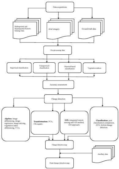
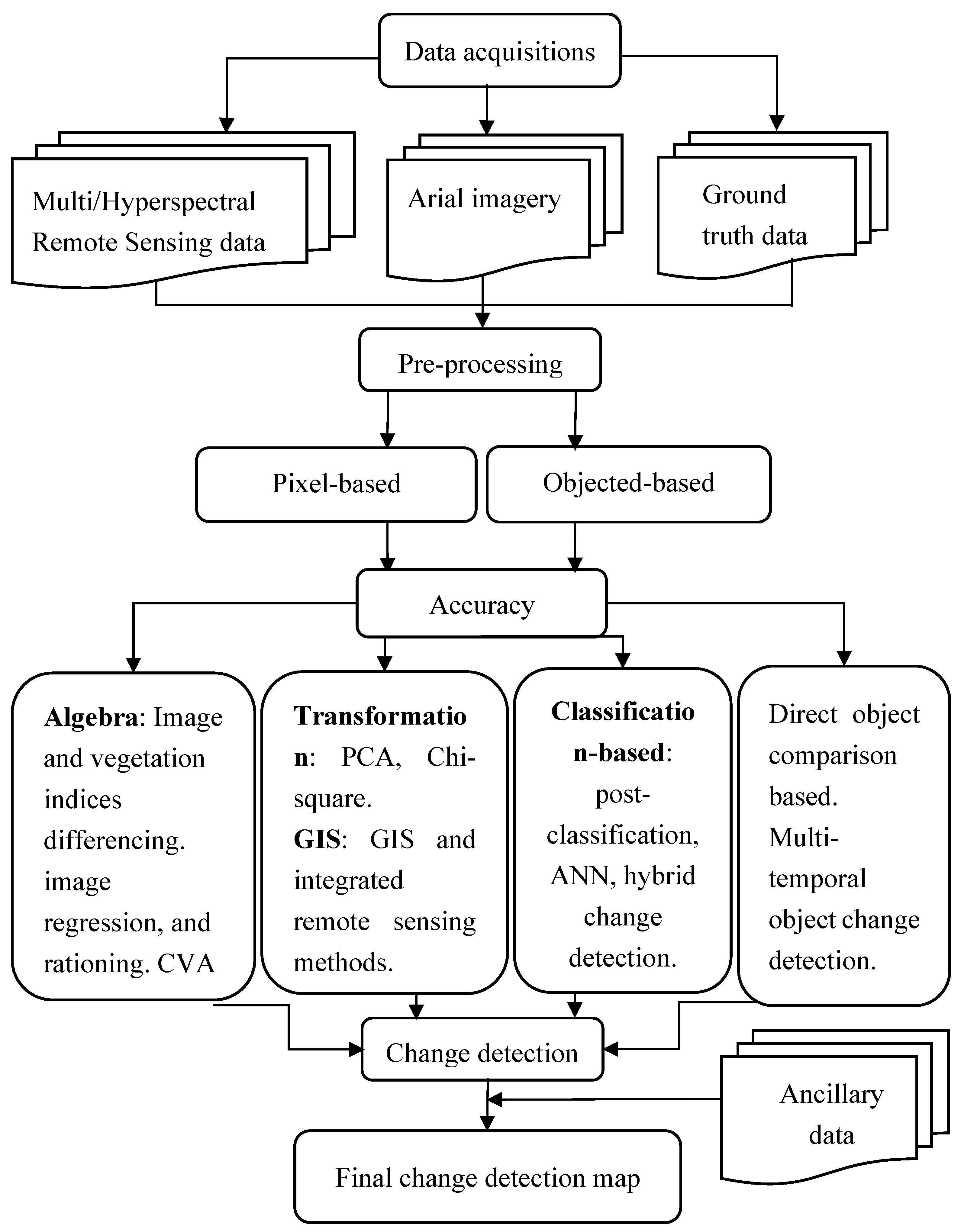
3. Mapping and Monitoring Vegetation Cover Change Using Remote Sensing Data

Using GIS and remote sensing technology has many advantages, such as saving time, large area coverage, and facilitating long-term monitoring with a faster implementation technique than ground methods [18]. Remote sensing techniques provide multispectral\hyperspectral images with resolutions that range from low to high. These remotely sensed data have been effectively used for mapping and monitoring vegetation cover change for a long period with mixed results [33]. Through the procedure of image interpretation and classification, remote sensing imagery covering a wide area at high temporal frequencies offers the opportunity to determine vegetation cover characteristics [34]. Remote sensing image classification techniques have been developed to generate updated vegetation cover information at various scales. Vegetation cover change classification is the method of considering each pixel as a labeled class to obtain the classified images [35]. Every pixel is considered a single entity and is assigned to a specific class through a pixel-based classification [17]. The heterogeneity of natural areas makes it increasingly necessary to utilize subpixel methods to better represent the mixture of land cover within a pixel [36]. Several methods have been developed for mapping sub-pixel land cover using remote sensing data [37,38]. Three improved methods were proposed by Niroumand et al. [39] to recover the spatial arrangement of land cover classes in images obtained from soft classification based on the original pixel-swapping method. According to Feng et al. [40], this method has an initialization that uses multiple subpixel-shifted mappings to reduce processing time and improve accuracy. There are several monitoring and detecting techniques for vegetation cover using remote sensing.

3.1. Supervised Classification

Supervised classification methods require analysts to input representative sample sites known as a training set. Based on the training set, spectral properties are compared for each pixel in the image and each pixel is labeled with a class type [34]. One of the main advantages of supervised classification is that errors can be detected and corrected. Additionally, when the analysts pick the training data, they may not highlight all conditions seen throughout the image, which may result in human error [41]. The supervised classification includes maximum likelihood classification (MLC), random forest classifier based on tree decision, support vector machine (SVM), spectral angle mapper (SAM), and artificial neural network (ANN). SVM is a machine learning technique based on statistical learning that can be used for classification and regression [42]. In MLC, pixels are classified based on the probability that they belong to a particular class. However, this method needs more computation time [43]. In complex landscape environments, mixed pixels are more likely to occur in the image. ANNs are based on biological neural networks and use statistical learning algorithms to learn [44]. Mustapha et al. [44] applied supervised classification for land cover in arid areas using MLC and ANN. Their results indicated that the ANN method yields better results than the MLC method and could overcome mixed pixels. Moreover, Jog and Dixit [42] used several supervised classification methods for vegetation cover. Their results indicated that SVM gave high accuracy of classification than MLC. Various tasks related to image processing can be solved using deep learning, which is a powerful machine learning methodology [45]. A growing number of studies have used deep learning to process remote sensing imagery over the past few years [46,47]. There is evidence that deep learning is effective for processing hyperspectral, multispectral, and radar images and for identifying different land cover types [48,49].

3.2. Unsupervised Classification

Unsupervised classification methods involve the selection of pixels from several areas or images, without using training data, for the identification of the types of phenomena observed [14]. In this approach, the algorithm divides the data without any previous knowledge and then employs thematic labels [16]. Unsupervised classification offers the advantages of being faster and free of human error, and the analyst does not require detailed prior knowledge [41]. Here, the data are clustered, and all pixels are then classified based on clusters. The unsupervised classification includes Iterative Self-Organizing Data Analysis (ISODATA) and K-means classification. ISODATA is one of the most popular unsupervised classification methods and is a reformation of the k-means. Basically, it requires three parameters: the number of classes in the classification process, the maximum number of iterations, and the convergence threshold [50]. Shivakumar [51] assessed the performance of unsupervised classification methods for LULC. Based on their findings, ISODATA classification techniques are more effective than K-means techniques at classifying LULCs. In addition, spectral dominant, as well as subservient classes, were successfully identified.

3.3. GEOBIA Classification

GEOBIA classification works by delineating geographic entities and investigating satellite image objects, rather than single pixels, by using the category of digital remote sensing image analysis [52]. Image objects are visually discernible elements and are usually represented by clusters of pixels that have a similar meaning, such as those represented by a tree’s crown or those representing crops in a field [53]. One of the unique features of GEOBIA compared to conventional per-pixel modeling techniques is that image objects (and not individual pixels) become the basic items of analysis because they represent meaningful geographical entities or phenomena at multiple scales [52]. Previous research has analyzed and classified images using dependent and independent variables to predict changes in vegetation cover in specific regions of the Earth’s surface [54]. The dependent variables for vegetation cover change prediction are the classified vegetation cover change map, while the independent variables are slope, elevation, aspect, water bodies, etc. [9].

3.4. Transform-Based Technique

In this type of change detection technique, the pixels of the image are transformed in order to determine if the image has changed [55]. Several popular transforms are commonly used today, including the Principal Component Analysis (PCA), the Tasseled Cap Transform, the Gramm–Schmidt Transform, and the Chi-Square Transform [56,57,58]. The main advantage of using the transform-based method for change detection is that it decreases redundant information between bands [55]. A transform-based change detection method utilizes the transform technique to perform a multiscale decomposition of the image. A separate component of the data is then separated from the independent component, and the separated component is then transformed into a component of the image [55]. A change map is then generated by threshold segmenting change components.

3.5. Geographic Information System (GIS)

GIS integrates information from a variety of sources to detect changes. GIS can be used to detect changes in an area by providing a larger view and frequent coverage of the area [55]. Prakash and Kumar [59] present an algorithm for detecting changes in the environment caused by natural disasters using remote sensing and GIS. Since GIS combines the quantitative data with the source data, it is much easier to extract and evaluate change detection information. Rawat and Kumar [60] described a method for detecting land cover changes by utilizing remote sensing and geographic information systems. They indicated that with the GIS approach, change detection could be made easier, more accurate, and less expensive.

3.6. Algebra-Based Technique

Using algebra-based change detection, each image pixel is subjected to mathematical operations to determine the difference image [55]. Image rationing, image differencing, and Change Vector Analysis (CVA) are some of the most used algebra-based change detection methods [55]. Except for CVA, the methods are relatively straightforward and easy to implement. For example, Xiong et al. [61] used a method of detecting change based on the likelihood ratio calculated from the joint Probability Density Function of the synthetic-aperture radar images. As discussed in Barber [62], the correlation coefficients of the synthetic-aperture radar images are computed using a generalized likelihood ratio test. Among the disadvantages of this method is the difficulty of classifying regions with low signal-to-noise ratios. Change detection techniques based on algebra are more easily implemented but do not provide a complete description of the changes detected [55].

Table 1. Classification and change detection techniques for detecting vegetation cover changes.

Techniques	Advantages	Disadvantages
Supervised classification	- Analyst has control. - Images can often be detected and corrected by the operator.	- Training data collection is a time-consuming and costly process. - A category that is not present in the training data cannot be recognized and represented.
Unsupervised Classification	- There are spectrally distinct areas that may not have been noticeable to the human eye. - There is no requirement for prior knowledge of the region. - Minimizes the possibility of human error.	- Analyses may not be able to relate spectral groups to information classes of interest. - The analyst has only limited control over the classes.
GEOBIA Classification	- A geographic feature in an image is treated as a set of objects rather than as an individual pixel. - Generation of vector data.	- Analyzing image. Parameters at the analyst’s discretion can introduce bias, which directly impacts the segmentation results.
Transform Based Technique	- It decreases redundant information between bands.	- Limited by the difficulty of labeling the information regarding the changing area.
Geographic Information System (GIS)	- Integrates information from multiple sources. - Coverage of the study area frequently and the ability to provide a broader view of it.	- Affected by the accuracy of information obtained from different sources.
Algebra-Based Technique	- Relatively straightforward and easy to implement except for CVA. - Reduce the impact from sensors, environment, sun angle, and atmosphere.	- Do not provide a complete description of the changes detected. - Accurate regression is required for the selected bands.

provids an overview of some classification and change detection techniques and their advantages and disadvantages.

4. Time Series Analysis for Monitoring Vegetation Cover Changes

Remote sensing data have been used for land cover monitoring since the first earth resources technology satellite (ERTS-1) was launched in 1972 [63]. A time series is a series of data collected at successive intervals over a certain period [64]. Additionally, for long-term monitoring using remote sensing data sequences, several studies have utilized remote sensing to monitor vegetation cover and land conditions over time [65,66,67]. In time-series analysis, methods are applied to understand the underlying forces structuring the data, identify patterns and trends, detect changes, cluster, model, and forecast the data [64]. Foran and Pearce [68] demonstrated that by using imagery from suitable dates, it is possible to monitor seasonal changes in vegetative cover in arid areas. Amri et al. [69] used a time series analysis of SPOT NDVI to assess vegetation behavior in a north African semi-arid region. They noted the potential for monitoring semi-arid vegetation cover resilience using satellite-time series data. Therefore, time series analysis is an excellent technique for characterizing vegetation canopy variation over time with a functional representation stable between years and continuous across seasons.

5. Using Vegetation Indices in Vegetation Cover Changes Studies

Different indices have been derived to use satellite data to detect changes in vegetation, and some of them include specific characteristics suitable for arid and semi-arid environments [18]. Commonly used multispectral and hyperspectral vegetation indices to detect changes in vegetation are shown in Table 2. The use of these indices in monitoring changes in vegetation cover has proven to be effective. Several spectral band combinations have been used to develop remote sensing-based vegetation indices for more than 20 years. As far as monitoring vegetation conditions are concerned, remote sensing-derived vegetation indices derived from land surface reflectance, such as the Normalized Differences Vegetation Index (NDVI) and Enhanced Vegetation Index (EVI), have been used often [70].

Karnieli et al. [71] proposed NDVI, one of the most extensively used vegetation indices for assessing vegetation cover. It was suggested by Rouse et al. [72] that it is more sensitive to detect green vegetation, even in areas with low vegetation cover. NDVI is sensitive to the different soil, atmospheric, and vegetation characteristics such as brightness, colors, cloud, cloud shadow, and leaf canopy shadow and requires remote sensing calibration [21]. Moreover, it can monitor the phenology, quantity, and activity of vegetation [73,74]. Somvanshi et al. [75] indicated that NDVI is sensitive to atmospheric effects and a smaller variety of spectral reflectance from vegetation. NDVI could be used to classify vegetated areas from non-vegetated ones, density of vegetation, and monitor and analyze seasonal variation in vigor and abundance in the vegetative state [75].

Table 2. Commonly used multispectral and hyperspectral vegetation indices to detect change in vegetation studies.

	Formula	Remarks	Reference
Multispectral Vegetation Index	Normalized Differences Vegetation Index $\mathrm{NDVI}=\frac{\left(\mathrm{NIR}-\mathrm{RED}\right)}{\left(\mathrm{NIR}+\mathrm{RED}\right)}$	NIR = reflection in the near-infrared band. RED = reflection in the red band. L = 1 no green vegetation cover, L = 0.5 in areas of moderate green vegetative cover. C1 = 6.0 atmospheric resistance coefficients. C2 = 7.5 atmospheric resistance coefficients BLUE = reflection in the blue band. vegetative cover. GREEN = reflection in the green band.	[74,76]
	Enhanced Vegetation Index $\mathrm{EVI}=2.5\times \frac{\left(\mathrm{NIR}-\mathrm{RED}\right)}{\left(\mathrm{NIR}+\mathrm{C}1\ast \mathrm{RED}-\mathrm{C}2\ast \mathrm{BLUE}+\mathrm{L}\right)}$		[74,76]
	Soil Adjusted Vegetation Index $\mathrm{SAVI}=\frac{\left(\mathrm{NIR}-\mathrm{RED}\right)}{\left(\mathrm{NIR}+\mathrm{RED}+\mathrm{L}\right)}\times \left(1+\mathrm{L}\right)$		[74,75]
	Atmospherically Resistant Vegetation Index $\mathrm{ARVI}=\frac{\left(\mathrm{NIR}-\left(2\times \mathrm{RED}-\mathrm{BLUE}\right)\right)}{\left(\mathrm{NIR}+\left(2\times \mathrm{RED}+\mathrm{BLUE}\right)\right)}$		[74,75]
	Ratio Vegetation Index RVI = NIR/RED		[18]
	Green Normalized Difference Vegetation Index $\mathrm{GNDVI}=\frac{\left(\mathrm{NIR}-\mathrm{GREEN}\right)}{\left(\mathrm{NIR}+\mathrm{GREEN}\right)}$		[18]
	Chlorophyll Index Green $\mathrm{CIgreen}=\frac{ \mathrm{NIR}}{\mathrm{GREEN}}-1$		[77]
	Difference Vegetation Index DVI = NIR − RED		[77]
	Chlorophyll Vegetation Index $\mathrm{CVI} =\frac{ \mathrm{NIR}}{\mathrm{GREEN}}\times \frac{ \mathrm{RED}}{\mathrm{GREEN}}$		[77]
	Optimized Soil Adjusted Vegetation Index $\mathrm{OSAVI}=\frac{1.16 \left(\mathrm{NIR}-\mathrm{RED}\right)}{ \mathrm{NIR}+\mathrm{RED}+0.16}$		[77]
	Transformed Vegetation Index $\mathrm{TVI}=\sqrt{(\frac{\mathrm{NIR}-\mathrm{RED}}{\mathrm{NIR}+\mathrm{RED}} })+0.5$		[18]
	Modified Transformed Vegetation Index $\mathrm{MTVI}=\sqrt{(\frac{\mathrm{c}\times \mathrm{NIR}-\mathrm{RED}}{\mathrm{c}\times \mathrm{NIR}+\mathrm{RED}} })$		[18]
Hyperspectral Vegetation Index	Normalized Differences Vegetation Index $\mathrm{NDVI}=\frac{\left(\mathrm{R}798-\mathrm{R}670\right)}{\left(\mathrm{R}798+\mathrm{R}670\right)}$	R670 = reflectance at 670 nm (%). R798 = reflectance at 798 nm (%).	[78]
	Enhanced Vegetation Index $\mathrm{EVI}=2.5\times \frac{\left(\mathrm{R}798-\mathrm{R}670\right)}{\left(\mathrm{R}798+\mathrm{C}1\times \mathrm{R}670-\mathrm{C}2\times \mathrm{R}470+\mathrm{L}\right)}$	L = 1 no green vegetation cover, L = 0.5 in areas of moderate green vegetative cover. C1 = 6.0 R670 = reflectance at 670 nm (%). R798 = reflectance at 798 nm (%). R470 = reflectance at 470 nm (%).	[79]
	Soil Adjusted Vegetation Index $\mathrm{SAVI}=\frac{\left(\mathrm{R}798-\mathrm{R}670\right)}{\left(\mathrm{R}798+\mathrm{R}670+\mathrm{L}\right)}\times \left(1+\mathrm{L}\right)$	L = 1 no green vegetation cover, L = 0.5 in areas of moderate green vegetative cover. R670 = reflectance at 670 nm (%). R798 = reflectance at 798 nm (%).	[80]
	Atmospherically Resistant Vegetation Index $\mathrm{ARVI}=\frac{\left(\mathrm{R}798-\left(2\times \mathrm{R}670-\mathrm{R}470\right)\right)}{\left(\mathrm{R}798+\left(2\times \mathrm{R}670+\mathrm{R}470\right)\right)}$	R670 = reflectance at 670 nm (%). R798 = reflectance at 798 nm (%). R470 = reflectance at 470 nm (%).	[74]
	Transformed Difference Vegetation Index $\mathrm{TDVI}=1.5 \frac{\mathrm{R}800-\mathrm{R}670}{\sqrt{(\mathrm{R}{800}^{2 }+\mathrm{R}670+0.5)}}$	R670 = reflectance at 670 nm (%). R800 = reflectance at 800 nm (%).	[78]
	Weighted Difference Vegetation Index $\mathrm{WDVI}=\mathrm{R}810 \left(\mathrm{crop}\right)-(\frac{\mathrm{R}810\left(\mathrm{soil}\right)}{\mathrm{R}560\left(\mathrm{soil}\right)}\times \mathrm{R}560 \left(\mathrm{crop}\right)$	R560 = reflectance at 560 nm (%). R810 = reflectance at 810 nm (%).	[74]
	Optimized Soil-adjusted Vegetation Index $\mathrm{OSAVI}=\left(\mathrm{R}800-\mathrm{R}670\right)\left(1+0.16\right)/\left(\mathrm{R}800+\mathrm{R}670+0.16\right)$	R670 = reflectance at 670 nm (%). R800 = reflectance at 800 nm (%).	[78]
	Modified Chlorophyll Absorption in Reflectance Index $\mathrm{MCARI}=\left[\left(\mathrm{R}700-\mathrm{R}600\right)-0.2 \left(\mathrm{R}700+\mathrm{R}600\right)\right]\left(\frac{\mathrm{R}700}{\mathrm{R}600}\right)$	R600 = reflectance at 600 nm (%). R700 = reflectance at 700 nm (%).	[78]

Table 2. Commonly used multispectral and hyperspectral vegetation indices to detect change in vegetation studies.

	Formula	Remarks	Reference
Multispectral Vegetation Index	Normalized Differences Vegetation Index $\mathrm{NDVI}=\frac{\left(\mathrm{NIR}-\mathrm{RED}\right)}{\left(\mathrm{NIR}+\mathrm{RED}\right)}$	NIR = reflection in the near-infrared band. RED = reflection in the red band. L = 1 no green vegetation cover, L = 0.5 in areas of moderate green vegetative cover. C1 = 6.0 atmospheric resistance coefficients. C2 = 7.5 atmospheric resistance coefficients BLUE = reflection in the blue band. vegetative cover. GREEN = reflection in the green band.	[74,76]
	Enhanced Vegetation Index $\mathrm{EVI}=2.5\times \frac{\left(\mathrm{NIR}-\mathrm{RED}\right)}{\left(\mathrm{NIR}+\mathrm{C}1\ast \mathrm{RED}-\mathrm{C}2\ast \mathrm{BLUE}+\mathrm{L}\right)}$		[74,76]
	Soil Adjusted Vegetation Index $\mathrm{SAVI}=\frac{\left(\mathrm{NIR}-\mathrm{RED}\right)}{\left(\mathrm{NIR}+\mathrm{RED}+\mathrm{L}\right)}\times \left(1+\mathrm{L}\right)$		[74,75]
	Atmospherically Resistant Vegetation Index $\mathrm{ARVI}=\frac{\left(\mathrm{NIR}-\left(2\times \mathrm{RED}-\mathrm{BLUE}\right)\right)}{\left(\mathrm{NIR}+\left(2\times \mathrm{RED}+\mathrm{BLUE}\right)\right)}$		[74,75]
	Ratio Vegetation Index RVI = NIR/RED		[18]
	Green Normalized Difference Vegetation Index $\mathrm{GNDVI}=\frac{\left(\mathrm{NIR}-\mathrm{GREEN}\right)}{\left(\mathrm{NIR}+\mathrm{GREEN}\right)}$		[18]
	Chlorophyll Index Green $\mathrm{CIgreen}=\frac{ \mathrm{NIR}}{\mathrm{GREEN}}-1$		[77]
	Difference Vegetation Index DVI = NIR − RED		[77]
	Chlorophyll Vegetation Index $\mathrm{CVI} =\frac{ \mathrm{NIR}}{\mathrm{GREEN}}\times \frac{ \mathrm{RED}}{\mathrm{GREEN}}$		[77]
	Optimized Soil Adjusted Vegetation Index $\mathrm{OSAVI}=\frac{1.16 \left(\mathrm{NIR}-\mathrm{RED}\right)}{ \mathrm{NIR}+\mathrm{RED}+0.16}$		[77]
	Transformed Vegetation Index $\mathrm{TVI}=\sqrt{(\frac{\mathrm{NIR}-\mathrm{RED}}{\mathrm{NIR}+\mathrm{RED}} })+0.5$		[18]
	Modified Transformed Vegetation Index $\mathrm{MTVI}=\sqrt{(\frac{\mathrm{c}\times \mathrm{NIR}-\mathrm{RED}}{\mathrm{c}\times \mathrm{NIR}+\mathrm{RED}} })$		[18]
Hyperspectral Vegetation Index	Normalized Differences Vegetation Index $\mathrm{NDVI}=\frac{\left(\mathrm{R}798-\mathrm{R}670\right)}{\left(\mathrm{R}798+\mathrm{R}670\right)}$	R670 = reflectance at 670 nm (%). R798 = reflectance at 798 nm (%).	[78]
	Enhanced Vegetation Index $\mathrm{EVI}=2.5\times \frac{\left(\mathrm{R}798-\mathrm{R}670\right)}{\left(\mathrm{R}798+\mathrm{C}1\times \mathrm{R}670-\mathrm{C}2\times \mathrm{R}470+\mathrm{L}\right)}$	L = 1 no green vegetation cover, L = 0.5 in areas of moderate green vegetative cover. C1 = 6.0 R670 = reflectance at 670 nm (%). R798 = reflectance at 798 nm (%). R470 = reflectance at 470 nm (%).	[79]
	Soil Adjusted Vegetation Index $\mathrm{SAVI}=\frac{\left(\mathrm{R}798-\mathrm{R}670\right)}{\left(\mathrm{R}798+\mathrm{R}670+\mathrm{L}\right)}\times \left(1+\mathrm{L}\right)$	L = 1 no green vegetation cover, L = 0.5 in areas of moderate green vegetative cover. R670 = reflectance at 670 nm (%). R798 = reflectance at 798 nm (%).	[80]
	Atmospherically Resistant Vegetation Index $\mathrm{ARVI}=\frac{\left(\mathrm{R}798-\left(2\times \mathrm{R}670-\mathrm{R}470\right)\right)}{\left(\mathrm{R}798+\left(2\times \mathrm{R}670+\mathrm{R}470\right)\right)}$	R670 = reflectance at 670 nm (%). R798 = reflectance at 798 nm (%). R470 = reflectance at 470 nm (%).	[74]
	Transformed Difference Vegetation Index $\mathrm{TDVI}=1.5 \frac{\mathrm{R}800-\mathrm{R}670}{\sqrt{(\mathrm{R}{800}^{2 }+\mathrm{R}670+0.5)}}$	R670 = reflectance at 670 nm (%). R800 = reflectance at 800 nm (%).	[78]
	Weighted Difference Vegetation Index $\mathrm{WDVI}=\mathrm{R}810 \left(\mathrm{crop}\right)-(\frac{\mathrm{R}810\left(\mathrm{soil}\right)}{\mathrm{R}560\left(\mathrm{soil}\right)}\times \mathrm{R}560 \left(\mathrm{crop}\right)$	R560 = reflectance at 560 nm (%). R810 = reflectance at 810 nm (%).	[74]
	Optimized Soil-adjusted Vegetation Index $\mathrm{OSAVI}=\left(\mathrm{R}800-\mathrm{R}670\right)\left(1+0.16\right)/\left(\mathrm{R}800+\mathrm{R}670+0.16\right)$	R670 = reflectance at 670 nm (%). R800 = reflectance at 800 nm (%).	[78]
	Modified Chlorophyll Absorption in Reflectance Index $\mathrm{MCARI}=\left[\left(\mathrm{R}700-\mathrm{R}600\right)-0.2 \left(\mathrm{R}700+\mathrm{R}600\right)\right]\left(\frac{\mathrm{R}700}{\mathrm{R}600}\right)$	R600 = reflectance at 600 nm (%). R700 = reflectance at 700 nm (%).	[78]

Liu et al. [79] analyzed several atmospheric-enhanced vegetation indices and soil types, such as the Atmospherically Resistant Vegetation Index (ARVI) and Soil-Adjusted Vegetation Index (SAVI; [21]). The SAVI is a vegetation index used to reduce the impact of soil brightness and color, using a soil brightness and color factor [81]. It is used for arid areas where vegetation cover is insignificant [21]. The ARVI is an enhanced index used to correct the impact of the atmosphere, useful in regions with a high atmospheric effect that consists of small particles of solids such as dust [82]. ARVI is less sensitive to atmospheric effects than NDVI [74]. However, due to atmospheric effects or the presence of large dust particles in the atmosphere, the ARVI index does not perform much better than NDVI if it is not computed using the 5S model [21]. Liu et al. [79] found that reducing one of the soils or the atmosphere may increase the other. Thus, they developed another index, the Enhanced Vegetation Index (EVI), to correct soil and atmospheric effects. Xue et al. [21] proposed an optimized EVI that improves the vegetation signal by decoupling the canopy background signal and reducing the atmospheric signal in high biomass regions, as well as improving vegetation monitoring. Moreover, EVI is more responsive to canopy variations, type, and architecture and can be responsive to vegetation stress and changes related to drought [21]. EVI can be used to monitor vegetation spatial and temporal variations and minimizes some of the problems related to NDVI.

NDVI and EVI use the near-infrared (NIR) wavelengths in which vegetation and water can always be separated [83]. As Moustafa et al. [84] pointed out, the benefit of EVI is that it includes the blue band, which helps reduce residual aerosols and atmospheric influences. For instance, dust near deserts and haze near arid coastlines are more responsive to NIR and canopy structural variations, such as canopy type, leaf area index, and architecture. However, NDVI is sensitive to chlorophyll and mostly to RED variations. Further, EVI can provide useful information about vegetation spatial and temporal variations, and minimize different problems in NDVI imagery such as contamination presence [84]. As found by Firouzi et al. [85], in a class with moderate vegetation, the EVI presented much greater vegetation values than the NDVI. However, in a class with sparse and dispersed vegetation, the NDVI presented vegetation values much higher than the EVI. NDVI values are also significantly correlated with vegetation coverage of three types—forest, shrubs, and grasslands—when judged by the R² value, as opposed to the EVI value [86].

EVI is more sensitive to differences in soil and atmospheric conditions [87]. There are many disadvantages to using such combinations, such as a lack of sensitivity to detect vegetation biomass, for example [88]. When vegetation indices are applied to heterogeneous canopy environments, such as horticultural and plantations, these limitations are especially evident [21]. There are soils, weeds, and covered crops in the intergrow, as well as plants of interest, making the determination of areas of interest and determining simple vegetation indices difficult. Moreover, variations in vegetation indices may be caused by different vegetation types in the area, as well as vegetation indices occurring in other vegetation similar to the subject vegetation [88].

Regression analysis of vegetation indices involves analyzing the relationship between the spectral index and the ecological variable used [89]. For example, as indicated in several studies, there is a strong correlation between the Leaf-Area Index (LAI) and NDVI [90,91]. Although the nature of the relationship varies throughout the studies, we cannot conclude that a given NDVI equals a given LAI in all cases. At low LAI, for example, the NDVI is heavily influenced by soil reflectance, and with increasing LAI, its sensitivity rapidly decreases due to asymptotic saturation. For example, Lawrence and Ripple [89] used two regression formulas assuming an NDVI of 0.5, and they found that the estimated LAI between two scenes differed by 5.5%. Using a relative sensitivity function, Ji and Peters. [92] compared the sensitivities of two vegetation indices without biophysical parameters. This technique is not limited to the analysis of vegetation indices but can also be applied to other variables associated with climatic, ecological, and environmental conditions.

6. Multi/Hyperspectral Satellite Sensors

6.1. Multispectral Satellite Sensors for Mapping and Monitoring Vegetation Cover Change

There have been many researchers conducted in the last three decades on the application of satellite imagery for monitoring and mapping vegetation cover changes, most of them using multispectral sensors. The multispectral satellites include but are not limited to Landsat Thematic Mapper (TM), Landsat Multispectral Scanner System (MSS), Enhanced Landsat Thematic Mapper (ETM+), Linear Imaging Self Scanning Sensor (LISS-III), Reflection Radiometer (Terra-ASTER), SPOT, Moderate Resolution Imaging Spectroradiometer (MODIS), Advanced Very High-Resolution Radiometer (AVHRR), IKONOS, QuickBird, and Sentinel-1 and -2.

Table 3. Commonly used multispectral satellite sensors.

Satellite Imagery	Bands	Temporal Resolution (Days)	Spatial Resolution (m)	Period	Data Access
Landsat MSS	4	180	80	1972–1992	https://earthexplorer.usgs.gov
TM Landsat	7	16	30, 120	1982–present	https://earthexplorer.usgs.gov
ETM+ Landsat	8	16	30, 15, 60	2003–present	https://earthexplorer.usgs.gov
Landsat OLI	11	16	30, 15	2013–present	https://earthexplorer.usgs.gov
Sentinel-1	C-band	12	5	2014–present 1A 2016–present 1B	https://scihub.copernicus.eu
Sentinel-2	13	5	60, 10, 20	2015–present 2A 2017–present 2B	https://scihub.copernicus.eu
MODIS	36	1–2	250, 500, 1000	2000–present Terra 2002–present Aqua	https://earthexplorer.usgs.gov https://search.earthdata.nasa.gov
AVHRR	5	1	1100–5000	1980–present	https://earthexplorer.usgs.gov
IKONOS	5	1–2	4	1999–2015	https://earth.esa.int
MERIS	15	3	300	2002–2012	https://earth.esa.int
QuickBird	5	1–3.5	2.4	2001–present	https://earth.esa.int
Rapid Eye	5	5.5	5	2008–2020	https://earth.esa.int
SPOT	4	26	10, 20	1986–2013	https://earth.esa.int
Worldview-2	8	1	<1	2014–present	https://earth.esa.int

lists the most used multispectral satellite sensors with low, medium, and high spatial resolutions.

In Table 3, spatial resolution refers to the pixel size in the satellite image for the ground. Arid and semi-arid vegetation cover is mostly scarce and sparsely distributed, making it difficult to detect using low and medium-resolution satellite remote sensing products. For example, MODIS and Advanced Very-High-Resolution Radiometer (AVHRR) satellite sensors have a low spatial resolution, which is equal to or greater than 250 m. Low spatial resolution images can be used for global scales and areas with a high density of vegetation. Knight et al. [93] used MODIS satellite imagery to assess the regional scale land cover characteristics of a study area of 52000 km² in North Carolina and Virginia.

Some other satellites, such as Landsat satellite imagery, have a medium spatial resolution, e.g., 30 m, which is acceptable when used to study vegetation in arid and semi-arid areas [11,94,95,96]. According to Zhang et al. [96], due to the complexity of land cover and the mixed-pixel problem in medium spatial resolution satellite images such as Landsat, especially in arid and semi-arid regions. Subpixel-based methods could be used to provide details of land cover change where previously pixel-based methods could not.

The worldview-2 mission has a very high spatial resolution of 1 m and can show details on the ground equal to or greater than 1 m, which is especially useful for arid and semi-arid areas with a sparse and low density of vegetation. Adam et al. [97] used high-resolution WorldView-2 for mapping Prosopis Glandulosa in the semi-arid environment of South Africa. Based on the results of their study, WorldView-2 imagery was able to map vegetation cover at the species level with remarkable accuracy. Moreover, merging medium spatial resolution, such as Landsat and Sentinel-1 imagery, with a spatial resolution of 5 m could be useful to better detect vegetation changes in arid and semi-arid areas and catch some key components of ground variation in which the density of components is less in arid environments [94].

The spectral resolution, on the other hand, refers to the number of wavelength detail in a band. Each spectral band uniquely detects a particular feature on the Earth’s surface by focusing its electromagnetic spectrum on a specific range. Multispectral satellite sensors provide two spectral resolutions: low and medium resolutions [98]. Moreover, most multispectral satellite sensors’ bands contain panchromatic, visible color (blue, green, red), and infrared bands. For example, Landsat-8 sensor spectral resolution contains a coastal aerosol, visible color, near-infrared, panchromatic, and short and long-wavelength infrared, which can produce 11 bands for each image. The QuickBird sensor contains only five bands, including panchromatic, visible color, and near-infrared. These multispectral bands have different applications; for example, red and near-infrared bands could be used for vegetation analysis, plant species and stress, and land use changes. Moreove, the combination of different bands, such as blue, near-infrared, and short-wave infrared, can investigate healthy vegetation.

The coverage period record of multispectral satellite sensors is also shown in Table 3. Landsat series and AVHRR images are the only sources of data that are suitable for studying vegetation cover changes in the past 40 years [99]. Landsat image has a medium spatial resolution and has been archived for a long time since 1972. However, some multispectral satellite sensors have a low coverage period record, such as Worldview-2, which was launched in 2014. Using only Worldview-2 images to detect vegetation cover changes can be limited because of the short period of time series detection. Most of the high-resolution satellite sensors were launched during the past 20 years, such as the Sentinel-1 series, QuickBird, and Rapid Eye. Some studies have combined two different sensors in their studies; for example, Zhang et al. [96] used Landsat ETM and QuickBird, while Bolton et al. [100] used Landsat with Sentinel-2 to detect the vegetation cover changes in arid and semi-arid regions. Combining low-middle resolution images with high-resolution images improves the visual quality and spatial resolution of images to emphasize certain properties. When merging datasets, it is important to note that some sensors have also currently retired, such as the Spot sensor, which was launched from 1986 to 2013 with two different spatial resolutions, medium and high, and therefore cannot be used over the entire study period or more real-time analysis.

The temporal resolution of multispectral satellite sensors refers to the time between the acquisition of two images of the same region. Some multispectral satellite sensors have a medium temporal resolution of about 16 days, such as Landsat sensors that show bi-monthly changes and not daily changes on the Earth’s surfaces. However, some sensors have a temporal resolution of 1 day, such as MODIS, which provides the change on the Earth’s surface day by day. A high temporal resolution could be useful to detect vegetation changes; however, it is important for other studies as well, such as weather studies where the change occurs from day to day. It is difficult to obtain satellite imagery that combines high temporal, spectral, and spatial resolution due to the narrow swath of satellite sensors. Therefore, data types needed for a particular study must be determined by researchers based on the objective of the work. High temporal resolution is essential when studying weather mechanisms, which change over time. On the other hand, seasonal vegetation changes may necessitate lower temporal resolution in favor of higher spatial or spectral resolution [101].

Multispectral Satellite Sample Applications

Satellite imagery with low spatial resolutions and a very high temporal resolution of 1 day, such as MODIS imagery (with a spatial resolution of 250, 500, and 1000 m) and AVHRR imagery (with spatial resolutions of 1100 m for local areas and 5000 m) were used in different literature for global studies [102,103,104,105,106]. They are used mostly for monitoring and mapping vegetation due to the high spectral resolution for big coverage areas due to their low spatial resolution [107]. For example, Duraisamy et al. [5] examined long-term land cover change at a finer scale in a semi-arid area of Mula Pravara in India. This study used AVHRR-NDVI data for the years 1982–2015 to identify the “hotspot” with major positive and negative aspects of vegetation cover change. Moreover, they used multi-temporal Landsat imagery to produce finer scale land cover maps and Support Vector Machines (SVM) supervised image classification was used to categorize the vegetation cover classes. This study results indicate that satellite remote sensing techniques are useful for monitoring the LUCC, which can be used to predict future land changes and aid in planning adaptation measures.

He et al. [108] used the AVHRR time series of annual land use and land cover vegetation maps of China from 1982 to 2013 to generate NDVI. They found that the overall accuracy of a simplified eight-class version of the 2012 land cover map is 73.8% success in vegetation classification, which is not considerably different from the accuracy of the MODIS map for the same year. Meanwhile, Yin et al. [102] used a time series of 250-m MODIS with a spectral resolution of 11 bands and a random forest classification method to study land cover vegetation changes between 2000 and 2014 in the arid desert of Inner Mongolia. NDVI and EVI time series were used as ancillary information, and the trajectory-based change detection method was applied in this study. They found that their trajectory-based method achieved high and accurate change detection, with an overall high accuracy of 0.95% success in vegetation classification. However, several limitations to this study; for example, the phenological and spectral similarities of grassland and cropland produced higher mapping errors and fine-scale land change processes were missed due to the spatial resolution of MODIS. Thus, compositing MODIS imagery with higher resolution archives can improve the detection of vegetation cover change at finer scales.

Medium-resolution satellite imagery with a low temporal resolution of 16 days, such as Landsat sensors, was used with data fusion and vegetation indices to investigate vegetation cover change in arid and semi-arid areas [13,95,109,110,111,112]. Hyvärinen et al. [109] used Landsat multispectral data (Landsat 5 and 8) with a spectral resolution of seven bands and spatial resolution of 30 m, SAVI, a supervised classification, and ground truth vegetation data to assess vegetation changes. This was performed to examine the long-term changes in vegetation productivity from 1987 to 2017 in South Africa. Their study results were limited as errors occurred in analyzing some vegetation types despite a high accuracy in their supervised classification. They recommended that higher spectral and spatial resolution in the remotely sensed data, together with radar-based products, might be useful for improving vegetation classification accuracy. Mohammed et al. [95] used Landsat ETM+ with a spatial resolution of 30 m to measure the spatial and temporal vegetation cover changes in Sudan and found that in complex areas characterized by a variety of complex features of the Earth’s surface, such as natural plants and crop areas, using medium spatial resolution data and mixed pixels can be problematic. A visual interpretation was used to address the issue of mixed pixels. Therefore, a visual interpretation of the resulting vegetation cover change maps is essential for enhancing classification accuracy and quality.

Some other studies have used either only medium-resolution multispectral satellite imagery or have combined medium-resolution multispectral satellite imagery with high-resolution multispectral satellite imagery [113,114,115,116]. For example, Teltscher and Fassnacht. [113] used medium multispectral Landsat with a spatial resolution of 30 m and high multispectral sentinel-2 satellite data of 10 m of spatial resolution to assess vegetation change at Mount St from 1984 to 2016. They applied a supervised random forest classification method on Sentinel-2 data due to the high spatial resolution to map the vegetation types. Moreover, change vector analysis was used with NDVI to assess the vegetation condition for the whole period. They concluded that to gain insight into a large area and examine a long period, the multispectral remote sensing imageries are extremely useful.

Many researchers have used high-resolution multispectral satellite imagery, such as spot-5 and QuickBird combined with field observations [117,118,119,120]. The purpose of combining field observations with remote sensing imagery is to validate the image signatures of soil, vegetation, water, etc., and increase accuracy. Al-Namazi and Almalki. [117] studied changes in vegetation cover over time in Mahazat Alsayd Natural Reserve and used remote sensing data and field observations to detect the vegetation coverage changes in the study area. SPOT-5 satellite data with a spatial resolution of 2.5 m were used to estimate NDVI in 2015. The results indicated that data fusion showed a significant decline in the vegetation cover of the study area from 1995 to 2015. Moreover, Elmahdy and Mohamed. [120] conducted a study to evaluate the vegetation cover change between 2000 and 2015 in Dubai using remote sensing data. The method was applied by collecting 320 training sample data using QuickBird satellite imagery with a high spatial resolution of 0.6 m, which was verified using field observations. They recommended that the field observations and high spatial resolution of multispectral satellite imagery improve accuracy for land cover classification.

6.2. Limitations of Multispectral Satellite Sensors in Vegetation Cover Change Mapping and Monitoring

Vegetation change studies use MODIS imagery extensively, but its low spatial resolution, which is equal to or more than 250 m, prevents it from being used to assess vegetation changes on small to medium spatial scales [11,121]. Combining MODIS imagery with higher spatial resolution imagery such as SPOT and QuickBird can provide more useful information for vegetation change monitoring at small to medium spatial scales [11,122]. However, QuickBrid and SPOT have very low spectral resolution ranges of four to five bands, while MODIS has high spectral bands of 36. Moreover, purchasing images with large numbers can be very expensive for multitemporal studies [123].

Landsat image series have various types of spectral sensors (TM and ETM+); thus, it is important for images acquired from Landsat sensors to have spectral reflectance correction, especially for long-time series vegetation cover [124]. Due to the limitation of Landsat spatial resolution images of 30 m, it is used for mapping vegetation at the community level instead of at the species level, as it would be difficult [125]. However, combing Landsat images with other high-resolution sensors and ancillary data, such as slope, elevation, aspect, water bodies, and soil data, can provide the possibility to use it to map at the species level [126]. As an example, Landsat images were combined with different environmental variables and forest management maps in the Amanos Mountains region of southern central Turkey to produce regional-scale vegetation maps [125].

Images from MODIS have a spatial resolution of 250 to 1000 m, including 36 spectral bands, and are predominantly used for vegetation dynamics mapping and processes [93]. However, it is not recommended to map vegetation at a regional scale due to the low spatial resolution [93]. Despite Landsat’s capabilities to map vegetation cover change and assess change dynamics, high spatial resolution satellite images such as QuickBird and IKONOS provide more detailed feature analysis and more accurate results when compared with Landsat images (TM, MSS, and ETM) [127]. However, hyperspectral images have overcome the incapability of multispectral images, especially when it comes to determining the various types of identical features, such as crops and plants. Therefore, they have been used for mapping and monitoring vegetation cover changes [128]. The difficulties in differentiating vegetation cover that results in similar vegetation cover features are also limited due to the similarity in reflectance across landscapes; for example, different vegetation with similar phenological characteristics may be indistinguishable [129].

6.3. Hyperspectral Satellite Sensors Data for Mapping and Monitoring Vegetation Cover Change

For monitoring and mapping vegetation cover changes, hyperspectral sensors have overcome many spectral limitations of multispectral satellite imagery. The hyperspectral sensor has several bands from the visible, near-infrared, mid-infrared, and short-wave infrared; for example, the visible and near-infrared bands range from one to 70 bands and allow for several combinations for calculating the narrow band for vegetation indices. Thus, different wavelengths of the spectral signatures and spatial analysis provide a comprehensive view of the objects.

As outlined in

Table 4. Commonly used hyperspectral satellite sensors.

Satellite Imagery	Bands	Temporal Resolution (day)	Spatial Resolution (m)	Launch Year
EO-1 (NASA)	242	16	30	2000
PROBA-1 (ESA)	150	7	34	2001
PRISMA (Italy)	250	29	30	2019
EnMap (Germany)	228	4	30	2020
HISUI (Japan)	185	2–60	30	2020
HypXIM (France)	210	3–5	10–20	2011
HJ-1A/B (China)	128	4	100	2008

, a hyperspectral sensor offers a wide range of spectral bands, such as the Earth Observing 1 (EO-1) sensor that can provide 242 bands with each spectral sensor band uniquely detecting a particular feature on the Earth’s surface, whereas multispectral imaging only assesses features on the Earth’s surface in a few bands. For example, hyperspectral sensors can be used to distinguish halophytic plants from non-halophytic plants and to identify salt features on the surface more precisely than is possible with a multispectral sensor [18]. Moreover, in hyperspectral imagery, vegetation reflectance is between green (670 nm) and near-infrared (800 nm). This spectral curve is known as the “red edge effect” [130]. Often, vegetation is distinguished from other land types by its “red edge effect,” and different vegetation types have different characteristics in the red edge range, and consequently, varying characteristic bands are selected while identifying species [130].

Hyperspectral narrow bands data exhibited greater efficiency and reliability than multispectral broadband data [131]. Using hyperspectral sensors, one can detect and monitor even subtle absorption features, such as the composition of leaves, the configuration of canopy structures, and the presence of disease in plants [132]. For example, to quantify constituents in plant leaves and detect subtle changes as a result of environmental stress, it is imperative that the sensor is highly sensitive to vegetation [131]. A subtle change in plant structure can therefore be detected in the Shortwave Infrared (SWIR), a region in the spectral range of 1100 to 2500 nm where most multispectral sensors offer limited resolution bands [133]. Using hyperspectral SWIR images, Cimtay et al. [134] proposed a new index algorithm to detect vegetation on land cover. A comparison of the proposed index algorithm results with the NDVI map has shown that it can produce very accurate results. Moreover, soil and water regions can also be detected successfully in hyperspectral images of the SWIR band. Kumar et al. [135] proposed a new vegetation index based on SWIR technology to detect changes in geographical features using multitemporal and multispectral satellite imagery. Landsat imagery has been used to develop the SWIR-based normalized difference vegetation index (SNDVI). The proposed vegetation index is a valuable tool for monitoring vegetation health and growth and detecting changes in vegetation.

In the context of coverage period records, hyperspectral sensors can only cover the past 20 years, such as The Project for On-Board Autonomy-1 (PROBA-1), which is limited compared to the multispectral satellite sensor. Until recently, the inadequate coverage period of detection of hyperspectral sensors has been a major limitation in their usage in change detection research. However, only some hyperspectral satellite sensors were launched in the previous 4 years. Thus, very limited studies were using hyperspectral sensors on vegetation cover changes, especially in arid and semi-arid areas. Different hyperspectral satellite sensors that were commonly used for vegetation cover changes studies are shown in Table 4. A few studies used some of the hyperspectral satellite sensors, especially in arid and semi-arid areas.

A hyperspectral image can map vegetation cover changes more effectively than a multispectral image because spectral properties provide more information about the features when compared to the multispectral data (Landsat ETM+, IKONOS, etc. [128]). In hyperspectral imaging, several hundred spectral bands are gathered in a single acquisition, which makes it more expensive to purchase because it requires more technology. However, multispectral sensors typically capture data from 3-15 spectral bands during one observation, and they can often be purchased for free or at a low cost. Thenkabail et al. [136] showed how hyperspectral data EO-1 has more power and better mapping accuracy by using narrowband data for biomass and land use or land cover classification. Nevertheless, as demonstrated by Bai et al. [137], Chutia et al. [138], and Liu and Li. [139], the availability of very high spectral and spatial resolutions may sometimes lead to erroneous results. It is challenging to classify hyperspectral remote sensing data accurately due to the enormous amount of information captured from the earth’s surface that is offered by many spectral bands [139].

One of the very useful techniques to collect imagery data, especially over the past few years with technological developments, is the use of an Unmanned Aircraft System (UAS). The platform consists of many types, including multi-rotors, swinglets, model helicopters, etc. [140]. Combined with imaging, ranging, and positioning sensors, these cameras can collect imagery at the cm-level resolution, providing an excellent opportunity to detect and monitor vegetation cover [141]. Various exciting and quantitative observations can be achieved with UAVs at a much greater spatial and temporal resolution and a lower cost than airborne platforms or satellites. UAV surveys enable us to capture remote images at very small pixel sizes, achieving higher resolution than aerial or satellite imagery [140]. In the context of airborne data, hyperspectral data from airborne surveys are generally obtained locally due to the increased cost of surveying [142]. Airborne systems have several advantages over satellite systems, such as the ability to choose dates and times for data acquisition to minimize atmospheric interference and change the spatial and spectral features of the data by changing altitudes and sensors as needed [143]. Hyperspectral airborne remote sensing is capable of mapping vegetation cover areas at a very detailed level in terms of spatial and spectral resolution, which is a valuable source of classification data [144].

UAVs and airborne can be equipped with HySpex VNIR and HySpex SWIR hyperspectral cameras. For example, Kluczek et al. [145] mapped the vegetation cover of the Tatra Mountains by combining airborne hyperspectral images acquired from HySpex with Sentinel-2 data. They indicated a high degree of similarity between maps obtained using HySpex imagery (2 m; 430 bands) and maps produced using multitemporal Sentinel-2 data (10 m; 132 bands; 11 acquisition dates). Therefore, it may be surprising that the results obtained with multitemporal Sentinel-2 data are comparable to those obtained with airborne HySpex data. An approach proposed by Helge et al. [146] for vegetation monitoring uses a 3-D representation of the surface in conjunction with hyperspectral data acquired by UAVs that shows the objects’ emitted and reflected light. The proposed approach enables the collection of complementary hyperspectral and 3D information using only one lightweight UAV imaging system.

Hyperspectral Satellite Sample Applications

Different researchers have used hyperspectral data, such as EO-1 Hyperion, to assess land cover vegetation in different places, for example, Australia, South America, and Asia [130,147,148]. Jafari and Lewis. [147] used EO-1 Hyperion hyperspectral data to assess arid land characterization. They mention that hyperspectral imagery may provide a better ability compared to multispectral imagery in distinguishing different vegetation types, especially when a low cover of vegetation is present. EO-1 Hyperion hyperspectral data were used in this study to evaluate their potential in identifying arid landscape elements in the southern rangelands of South Australia. A spectral mixture analysis was performed on Hyperion imagery to identify the components of vegetation cover changes that differ spectrally. A spectral mixture analysis in this arid environment was not able to detect more than five spectral endmembers, despite the high spectral resolution of the Hyperion scene. There may be three reasons for this: low coverage of vegetation (28%) in the region, the lack of spectral contrast in arid vegetation types, and the low ground resolution of Hyperion (900 m²).

Over forest areas with a high density of trees, Millán et al. [149] mapped tropical dry forest succession in Brazil using Compact High-Resolution Imaging Spectrometer (CHRIS) and PROBA-1 hyperspectral images. This was achieved by exploring the best seasons, such as wet or dry seasons, and the angle of observation. Classification maps were built using nonparametric decision trees based on Principal Component Analysis (PCA) inputs. Ten CHRIS/PROBA images were obtained: five images corresponding to the end of the dry season and the others corresponding to the end of the wet season. The authors indicated in their discussion that CHRIS/PROBA images can provide information about the canopy and the understory elements during the dry season.

Different studies have used Environmental Mapping and Analysis Program (EnMap) hyperspectral sensor to assess vegetation cover in semi-arid areas in Europe [150,151,152]. Suess et al. [152] focused on the semi-arid natural environment in Portugal to examine shrub vegetation along a gradient of shrub encroachment. EnMAP satellite data pertaining to shrub vegetation within the study area were used to map shrub vegetation and a support vector classification (SVC) model was used to obtain information regarding shrub cover fractions. As a result, shrub vegetation maps depict gradual transitions more realistically. As hyperspectral satellite data are relevant for mapping natural ecosystems, SVC is valuable in describing gradual transitions in shrub vegetation qualitatively and quantitatively. Hyperspectral satellite data being relevant for mapping natural ecosystems, SVC has value in describing gradual transitions in shrub vegetation qualitatively and quantitatively.

7. Vegetation Cover Change Analysis

Figure 1 shows the typical workflow of vegetation cover change analysis in the field of remote sensing and GIS. Different types of data acquisition could be used as single or fusion data, such as multispectral and hyperspectral remote sensing, aerial imagery, ground truth data, radar, and LiDAR data. The main data types on remote sensing are obtained from satellites and aircraft. Some data are easy to collect over a variety of scales and resolutions, such as Landsat sensors data. Researchers may use a single sensor data of remote sensing or combine multiple remote sensing data for mapping and monitoring vegetation cover. Combined data from different sources are useful for improving the potential values. Pre-processing operations on remote sensing data are implemented after acquiring the remote sensing data and can include image restoration and rectification. In this pre-processing step, data distortions arising from radiometric and geometric sensors need to be corrected. Vegetation cover classification and vegetation indices calculation are the most important step after pre-processing of data.

The image classification method can be selected based on the resolution data and object characteristics. Supervised and unsupervised image classification is the most common technique. Object-based image classification is useful mostly for high-resolution data. Different classification methods (discussed in Section 3.1, Section 3.2 and Section 3.3) have been used by researchers to classify satellite imagery features [1,153,154,155,156]. An important step after image classification is accuracy assessment. Comparing the classified image with another ground truth or accurate data source.

Change detection is the difference between multiple raster datasets after the process of classification and calculating vegetation indices. Different change detection methods have been used by researchers for analyzing vegetation cover changes and are depicted in Figure 1 [157,158,159,160,161,162,163,164]. These change detection techniques use thresholds to distinguish between unchanged and changed areas. Image differencing in the Algebra change detection technique is most often used for vegetation change detection in arid and semi-arid areas, which is a simple and straightforward method, with results that are easy to understand [165]. Moreover, the use of GIS for change detection has also proved useful in a wide range of applications, especially when multiple sources of data are being used [165]. More details of change detection techniques could be found in [165]. After calculating the change detection between two or several images, the final change detection map will be produced.

8. Challenges in Mapping Vegetation Cover Changes in Arid and Semi-Arid Regions Using Remote Sensing

The vegetation information extracted from remote sensing has some limitations and significant challenges. Both spatial and temporal variabilities in the vegetation regions are limiting factors in mapping and assessing vegetation cover changes using remote sensing data due to spectral reflectance. It is incapable of specifying the information on the whole vegetation region and observes only the vegetation surface, regardless of whether it is perennials or plants that germinate only after the rain [166]. When an area is covered by a variety of vegetation types, it sometimes causes similar spectral reflectance across different types of vegetation and sometimes varying spectral reflectance within a single type of vegetation [126,167]. However, there are no super image classifiers that can apply uniformly to all applications, despite some standard methods for image pre-processing [126]. Moreover, the use of ancillary data, such as geographic information system data layers, has proved very useful for improving classification accuracy or obtaining a more satisfactory result [168]. Nevertheless, ancillary data cannot solve all difficulties faced during vegetation extraction from remote sensing data and will only improve the results [18,126].

Moreover, plants’ adaptations to their surroundings have a lot to do with the radiation environment present there, for example, the intense sun and heat, which directly affect the characteristics of the vegetation’s spectral distribution [169,170]. One of the most distinctive features of semi-arid environments is the variation in precipitation and fluctuation in rainfall, which affect plant growth both on a seasonal and a year-to-year basis [166,171]. In arid and semi-arid environments, plants are exposed to extreme weather conditions and must survive prolonged aridity, involving little or no rain for several years together. Compared to perennials, annuals germinate only after rain and a lot of water, which may affect the interpretation of the images they produce [166].

9. Multisource and Multitemporal Data Fusion

Most existing studies that used remote sensing data to detect vegetation cover changes have applied only a single sensor or image. That may not be adequate for complex applications such as detecting the changes in vegetation cover [172]. Remote sensing data comes from various sensors, each with its own characteristics, along with GIS data and ground truth data. Thus, it would be useful if they were merged to give a more comprehensive picture of the observable sites [172]. Multi-source data are combined data from different sources to improve the potential values and interpretations of the source data, and to produce an improved visual representation of the source data such as optical images, Synthetic-Aperture Radar (SAR), LiDAR, GIS data, and ground truth data [173]. Multitemporal data are a time series with several images or at least a pair of images for the same geographical study area at different times [174]. For instance, by merging optical and radar data, one could reduce the problems of mixed pixels and data saturation, while improving biomass estimations [172].

In the context of multi-source and multi-temporal data, various methods have been developed to integrate spectral and spatial information from different sensors, for improving the quality of visual interpretation and measurable analysis through data fusion [173,174]. Multispectral imagery combined with LiDAR data has also been used to produce better forest classifications in several studies on vegetation cover changes [175]. Remote sensing data combined with GIS data, such as topography, land use, and census data, can enhance the accuracy of object recognition, image classification, and change detection. Such a combination has played a key role in map updating, according to previous research [15,176]. Image data are typically composed of pixels, whereas GIS data are made up of objects with labels indicating their affiliation with regions. GIS data may be utilized as additional bands in post-processing and the selection of training areas to incorporate GIS data as auxiliary information [173]. Vegetation cover changes map requires the acquisition of multi-temporal profiles of change detection; therefore, images of multiple dates need to be acquired to generate a vegetation cover changes map, to overcome data missing due to any technical problems when dealing with a large study area. An ancillary data set such as MODIS aids in predicting and filling-in missing values in Landsat time series [177].

Arid and semi-arid ecosystems have small and sparsely distributed vegetation patches, making them difficult to detect with satellite remote sensing. It might be possible to detect tall vegetation species with small canopies using high-resolution multispectral data. For modeling vegetation canopy height and bare earth surface, LiDAR is commonly used as a three-dimensional active sensor. By combining LiDAR and multispectral data, it can be estimated both horizontal vegetation and bare ground cover and the vertical structure of vegetation [178].

10. Conclusions

Vegetation cover changes are a global environmental phenomenon occurring naturally or through human activities. Monitoring this is especially important in arid and semi-arid regions due to plant cover’s scarce and sensitive nature. The consequences of vegetation cover change may transform naturally vegetated areas into bare areas, impacting the environmental system. These changes being one of the most severe environmental concerns facing humanity, the early detection of vegetation cover changes and assessment of their extent and severity on local and regional scales becomes very important. Traditionally, vegetation cover changes were assessed through field campaigns and the collection of samples for laboratory analysis, which is a costly and time-consuming process, especially over a large study area.

Remote sensing is an alternative way of monitoring and detecting vegetation cover changes. Multispectral satellite sensors are ideal for mapping and monitoring vegetation cover changes, mostly due to their low cost and the relatively high availability of such images. Moreover, visual interpretation of the resulting vegetation cover change maps is essential for enhancing classification accuracy and quality. A high spatial resolution multispectral imagery is recommended to detect vegetation changes in arid and semi-arid areas. Using additional data jointly with satellite imagery, such as aerial imagery and ground truth data, can improve accuracy in monitoring and mapping vegetation cover.

Moreover, including ancillary data such as slope, elevation, aspect, water bodies, and soil with satellite imagery data can detect vegetation cover changes at the species levels. Higher spectral and spatial resolution remotely sensed data used jointly with radar-based products might be useful for improving vegetation classification accuracy. By classifying images, thematic maps are generated based on remote sensing data. However, due to their spectral and spatial resolution, some multispectral satellite data have limited abilities. Hyperspectral satellite imagery can largely overcome this limitation due to its better spectral resolutions. In addition, vegetation indices are developed through different research studies to detect and map areas with vegetation cover changes. Vegetation indices have different vegetation detection capabilities and have been applied for different purposes and areas. Considering a single vegetation index alone may not detect vegetation change accurately. Before using appropriate remote sensing-based indices for mapping and assessing vegetation cover changes, each site must be assessed to identify the strengths and weaknesses of the proposed indices.

References

1. Alam, A.; Bhat, M.S.; Maheen, M. Using Landsat satellite data for assessing the land use and land cover change in Kashmir valley. GeoJournal 2020, 85, 1529–1543. [Google Scholar] [CrossRef] [Green Version]
2. Ramankutty, N.; Foley, J.A. Estimating historical changes in global land cover: Croplands from 1700 to 1992. Glob. Biogeochem. Cycles 1999, 13, 997–1027. [Google Scholar] [CrossRef]
3. Khan, Z.; Saeed, A.; Bazai, M.H. Land use/land cover change detection and prediction using the CA-Markov model: A case study of Quetta city, Pakistan. J. Geogr. Soc. Sci. 2020, 2, 164–182. [Google Scholar]
4. Fathizad, H.; Rostami, N.; Faramarzi, M. Detection and prediction of land cover changes using Markov chain model in semi-arid rangeland in western Iran. Environ. Monit. Assess. 2015, 187, 629. [Google Scholar] [CrossRef]
5. Duraisamy, V.; Bendapudi, R.; Jadhav, A. Identifying hotspots in land use land cover change and the drivers in a semi-arid region of India. Environ. Monit. Assess. 2018, 190, 535. [Google Scholar] [CrossRef] [Green Version]
6. Ghaffar, A. Use of geospatial techniques in monitoring urban expansion and land use change analysis: A case of Lahore, Pakistan. J. Basic Appl. Sci. 2015, 11, 265–273. [Google Scholar]
7. Wu, Q.; Li, H.-Q.; Wang, R.-S.; Paulussen, J.; He, Y.; Wang, M.; Wang, B.-H.; Wang, Z. Monitoring and predicting land use change in Beijing using remote sensing and GIS. Landsc. Urban Plan. 2006, 78, 322–333. [Google Scholar] [CrossRef]
8. Reis, S. Analyzing land use/land cover changes using remote sensing and GIS in Rize, North-East Turkey. Sensors 2008, 8, 6188–6202. [Google Scholar] [CrossRef] [Green Version]
9. Liping, C.; Yujun, S.; Saeed, S. Monitoring and predicting land use and land cover changes using remote sensing and GIS techniques—A case study of a hilly area, Jiangle, China. PLoS ONE 2018, 13, e0200493. [Google Scholar] [CrossRef]
10. Kennedy, R.E.; Cohen, W.B.; Schroeder, T.A. Trajectory-based change detection for automated characterization of forest disturbance dynamics. Remote Sens. Environ. 2007, 110, 370–386. [Google Scholar] [CrossRef]
11. Yang, Z.; Shen, Y.; Jiang, H.; Feng, F.; Dong, Q. Assessment of the environmental changes in arid and semiarid mining areas using long time-series Landsat images. Environ. Sci. Pollut. Res. 2021, 28, 52147–52156. [Google Scholar] [CrossRef] [PubMed]
12. Rundquist, D.C. Field techniques in remote sensing: Learning by doing. Geocarto Int. 2001, 16, 85–90. [Google Scholar] [CrossRef]
13. Cui, X.; Gibbes, C.; Southworth, J.; Waylen, P. Using remote sensing to quantify vegetation change and ecological resilience in a semi-arid system. Land 2013, 2, 108–130. [Google Scholar] [CrossRef] [Green Version]
14. Alqurashi, A.; Kumar, L. Investigating the use of remote sensing and GIS techniques to detect land use and land cover change: A review. Adv. Remote Sens. 2013, 2, 193–204. [Google Scholar] [CrossRef] [Green Version]
15. Aydöner, C.; Maktav, D. The role of the integration of remote sensing and GIS in land use/land cover analysis after an earthquake. Int. J. Remote Sens. 2009, 30, 1697–1717. [Google Scholar] [CrossRef]
16. Huang, X.; Jensen, J.R. A machine-learning approach to automated knowledge-base building for remote sensing image analysis with GIS data. Photogramm. Eng. Remote Sens. 1997, 63, 1185–1193. [Google Scholar]
17. MohanRajan, S.N.; Loganathan, A.; Manoharan, P. Survey on Land Use/Land Cover (LU/LC) change analysis in remote sensing and GIS environment: Techniques and Challenges. Environ. Sci. Pollut. Res. 2020, 27, 29900–29926. [Google Scholar] [CrossRef] [PubMed]
18. Allbed, A.; Kumar, L. Soil salinity mapping and monitoring in arid and semi-arid regions using remote sensing technology: A review. Adv. Remote Sens. 2013, 2013, 41262. [Google Scholar] [CrossRef] [Green Version]
19. Karabulut, M. An examination of spectral reflectance properties of some wetland plants in Göksu Delta, Turkey. J. Int. Environ. Appl. Sci. 2018, 13, 194–203. [Google Scholar]
20. Foley, W.J.; McIlwee, A.; Lawler, I.; Aragones, L.; Woolnough, A.P.; Berding, N. Ecological applications of near infrared reflectance spectroscopy–a tool for rapid, cost-effective prediction of the composition of plant and animal tissues and aspects of animal performance. Oecologia 1998, 116, 293–305. [Google Scholar] [CrossRef]
21. Xue, J.; Su, B. Significant remote sensing vegetation indices: A review of developments and applications. J. Sens. 2017, 2017, 1353691. [Google Scholar] [CrossRef] [Green Version]
22. Humphries, M.S.; Kindness, A.; Ellery, W.N.; Hughes, J.C.; Bond, J.K.; Barnes, K.B. Vegetation influences on groundwater salinity and chemical heterogeneity in a freshwater, recharge floodplain wetland, South Africa. J. Hydrol. 2011, 411, 130–139. [Google Scholar] [CrossRef]
23. Loik, M.; Breshears, D.; Lauenroth, W.; Belnap, J. Climatology and ecohydrology of precipitation pulses in arid and semiarid ecosystems of the western USA. Oecologia 2004, 141, 269–281. [Google Scholar] [CrossRef] [PubMed]
24. Schwinning, S.; Sala, O.E. Hierarchy of responses to resource pulses in arid and semi-arid ecosystems. Oecologia 2004, 141, 211–220. [Google Scholar] [CrossRef]
25. Cui, M.; Caldwell, M.M. A large ephemeral release of nitrogen upon wetting of dry soil and corresponding root responses in the field. Plant Soil 1997, 191, 291–299. [Google Scholar] [CrossRef]
26. Stow, D.A.; Hope, A.; McGuire, D.; Verbyla, D.; Gamon, J.; Huemmrich, F.; Houston, S.; Racine, C.; Sturm, M.; Tape, K. Remote sensing of vegetation and land-cover change in Arctic Tundra Ecosystems. Remote Sens. Environ. 2004, 89, 281–308. [Google Scholar] [CrossRef] [Green Version]
27. Markon, C.J.; Fleming, M.D.; Binnian, E.F. Characteristics of vegetation phenology over the Alaskan landscape using AVHRR time-series data. Polar Rec. 1995, 31, 179–190. [Google Scholar] [CrossRef]
28. Leprieur, C.; Kerr, Y.; Mastorchio, S.; Meunier, J. Monitoring vegetation cover across semi-arid regions: Comparison of remote observations from various scales. Int. J. Remote Sens. 2000, 21, 281–300. [Google Scholar] [CrossRef]
29. Arkebauer, T.J. Leaf radiative properties and the leaf energy budget. Micrometeorol. Agric. Syst. 2005, 47, 93–103. [Google Scholar]
30. Olioso, A.; Sòria, G.; Sobrino, J.; & Duchemin, B. Evidence of low land surface thermal infrared emissivity in the presence of dry vegetation. IEEE Geosci. Remote Sens. Lett. 2007, 4, 112–116. [Google Scholar] [CrossRef] [Green Version]
31. Deval, K.; Joshi, P. Vegetation type and land cover mapping in a semi-arid heterogeneous forested wetland of India: Comparing image classification algorithms. Environ. Dev. Sustain. 2022, 24, 3947–3966. [Google Scholar] [CrossRef]
32. Abdullah, M.M.; Gholoum, M.M.; Abbas, H.A. Satellite vs. UAVs remote sensing of arid ecosystems: A review with in an ecological perspective. Environ. Anal. Ecol. Stud. 2018, 2, 1–5. [Google Scholar]
33. Aplin, P. Remote sensing: Land cover. Prog. Phys. Geogr. 2004, 28, 283–293. [Google Scholar] [CrossRef]
34. Li, M.; Zang, S.; Zhang, B.; Li, S.; Wu, C. A review of remote sensing image classification techniques: The role of spatio-contextual information. Eur. J. Remote Sens. 2014, 47, 389–411. [Google Scholar] [CrossRef]
35. Dingle Robertson, L.; King, D.J. Comparison of pixel-and object-based classification in land cover change mapping. Int. J. Remote Sens. 2011, 32, 1505–1529. [Google Scholar] [CrossRef]
36. MacLachlan, A.; Roberts, G.; Biggs, E.; Boruff, B. Subpixel land-cover classification for improved urban area estimates using Landsat. Int. J. Remote Sens. 2017, 38, 5763–5792. [Google Scholar] [CrossRef]
37. Tatem, A.J.; Lewis, H.G.; Atkinson, P.M.; Nixon, M.S. Super-resolution target identification from remotely sensed images using a Hopfield neural network. IEEE Trans. Geosci. Remote Sens. 2001, 39, 781–796. [Google Scholar] [CrossRef] [Green Version]
38. Verhoeye, J.; de Wulf, R. Sub-Pixel Mapping of Sahelian Wetlands using Multi-Temporal Spot Vegetation Images; Laboratory of Forest Management and Spatial Information Techniques Faculty of Agricultural and Applied Biological Sciences, University of Gent: Ghent, Belgium, 2000. [Google Scholar]
39. Niroumand Jadidi, M.; Safdarinezhad, A.; Sahebi, M.; Mokhtarzade, M. A novel approach to super resolution mapping of multispectral imagery based on pixel swapping technique. ISPRS Annals of Photogrammetry. Remote Sens. Spat. Inf. Sci. 2012, 7, 159–164. [Google Scholar]
40. Ling, F.; Du, Y.; Xiao, F.; Xue, H.; Wu, S. Super-resolution land-cover mapping using multiple sub-pixel shifted remotely sensed images. Int. J. Remote Sens. 2010, 31, 5023–5040. [Google Scholar] [CrossRef]
41. Nath, S.S.; Mishra, G.; Kar, J.; Chakraborty, S.; Dey, N. A survey of image classification methods and techniques. In Proceedings of the 2014 International Conference on Control, Instrumentation, Communication and Computational Technologies (ICCICCT), Kanyakumari District, India, 10–11 July 2014; IEEE: Piscataway, NJ, USA, 2014. [Google Scholar]
42. Jog, S.; Dixit, M. Supervised classification of satellite images. In Proceedings of the 2016 Conference on Advances in Signal Processing (CASP), Pune, India, 9–11 June 2016; IEEE: Piscataway, NJ, USA, 2016. [Google Scholar]
43. Al-Ahmadi, F.; Al-Hames, A. Comparison of four classification methods to extract land use and land cover from raw satellite images for some remote arid areas, Kingdom of Saudi Arabia. Earth Sci. 2009, 20, 167–191. [Google Scholar] [CrossRef]
44. Mustapha, M.; Lim, H.; Jafri, M.M. Comparison of neural network and maximum likelihood approaches in image classification. J. Appl. Sci. 2010, 10, 2847–2854. [Google Scholar] [CrossRef] [Green Version]
45. Kussul, N.; Lavreniuk, M.; Skakun, S.; Shelestov, A. Deep learning classification of land cover and crop types using remote sensing data. IEEE Geosci. Remote Sens. Lett. 2017, 14, 778–782. [Google Scholar] [CrossRef]
46. Zhang, F.; Du, B.; Zhang, L. Saliency-guided unsupervised feature learning for scene classification. IEEE Trans. Geosci. Remote Sens. 2014, 53, 2175–2184. [Google Scholar] [CrossRef]
47. Zhang, F.; Du, B.; Zhang, L. Scene classification via a gradient boosting random convolutional network framework. IEEE Trans. Geosci. Remote Sens. 2015, 54, 1793–1802. [Google Scholar] [CrossRef]
48. Mnih, V.; Hinton, G.E. Learning to detect roads in high-resolution aerial images. In Proceedings of the European Conference on Computer Vision, Crete, Greece, 5–11 September 2010; Springer: Berlin/Heidelberg, Germany, 2010. [Google Scholar]
49. Geng, J.; Fan, J.; Wang, H.; Ma, X.; Li, B.; Chen, F. High-resolution SAR image classification via deep convolutional autoencoders. IEEE Geosci. Remote Sens. Lett. 2015, 12, 2351–2355. [Google Scholar] [CrossRef]
50. Abburu, S.; Golla, S.B. Satellite image classification methods and techniques: A review. Int. J. Comput. Appl. 2015, 119, 20–25. [Google Scholar] [CrossRef]
51. Shivakumar, B. Land Cover Mapping Capability of Chaincluster, K-Means, and ISODATA techniques—A Case Study. In Advances in VLSI, Signal Processing, Power Electronics, IoT, Communication and Embedded Systems; Springer: Berlin/Heidelberg, Germany, 2021; pp. 273–288. [Google Scholar]
52. Chen, G.; Weng, Q.; Hay, G.J.; He, Y. Geographic object-based image analysis (GEOBIA): Emerging trends and future opportunities. GISci. Remote Sens. 2018, 55, 159–182. [Google Scholar] [CrossRef]
53. Hay, G.J.; Castilla, G.; Wulder, M.A.; Ruiz, J.R. An automated object-based approach for the multiscale image segmentation of forest scenes. Int. J. Appl. Earth Obs. Geoinf. 2005, 7, 339–359. [Google Scholar] [CrossRef]
54. Navin, M.S.; Agilandeeswari, L. Multispectral and hyperspectral images based land use/land cover change prediction analysis: An extensive review. Multimed. Tools Appl. 2020, 79, 29751–29774. [Google Scholar] [CrossRef]
55. Asokan, A.; Anitha, J. Change detection techniques for remote sensing applications: A survey. Earth Sci. Inform. 2019, 12, 143–160. [Google Scholar] [CrossRef]
56. Sadeghi, V.; Ahmadi, F.F.; Ebadi, H. Design and implementation of an expert system for updating thematic maps using satellite imagery (case study: Changes of Lake Urmia). Arab. J. Geosci. 2016, 9, 257. [Google Scholar] [CrossRef]
57. Thakkar, A.K.; Desai, V.R.; Patel, A.; Potdar, M.B. An effective hybrid classification approach using tasseled cap transformation (TCT) for improving classification of land use/land cover (LU/LC) in semi-arid region: A case study of Morva-Hadaf watershed, Gujarat, India. Arab. J. Geosci. 2016, 9, 180. [Google Scholar] [CrossRef]
58. Vázquez-Jiménez, R.; Romero-Calcerrada, R.; Novillo, C.J.; Ramos-Bernal, R.N.; Arrogante-Funes, P. Applying the chi-square transformation and automatic secant thresholding to Landsat imagery as unsupervised change detection methods. J. Appl. Remote Sens. 2017, 11, 016016. [Google Scholar] [CrossRef]
59. Maurya, S.P.; Yadav, A.K. Evaluation of course change detection of Ramganga river using remote sensing and GIS, India. Weather Clim. Extrem. 2016, 13, 68–72. [Google Scholar] [CrossRef] [Green Version]
60. Rawat, J.; Kumar, M. Monitoring land use/cover change using remote sensing and GIS techniques: A case study of Hawalbagh block, district Almora, Uttarakhand, India. Egypt J. Remote Sens. Space Sci. 2015, 18, 77–84. [Google Scholar] [CrossRef] [Green Version]
61. Xiong, B.; Chen, J.M.; Kuang, G. A change detection measure based on a likelihood ratio and statistical properties of SAR intensity images. Remote Sens. Lett. 2012, 3, 267–275. [Google Scholar] [CrossRef]
62. Barber, J. A generalized likelihood ratio test for coherent change detection in polarimetric SAR. IEEE Geosci. Remote Sens. Lett. 2015, 12, 1873–1877. [Google Scholar] [CrossRef]
63. Jafari, R. Arid Land Condition Assessment and Monitoring using Mulitspectral and Hyperspectral Imagery. Ph.D. Thesis, School of Earth and Environmental Sciences, University of Adelaide, Adelaide, Australia, 2007. [Google Scholar]
64. Van Den Bergh, F.; Wessels, K.J.; Miteff, S.; Van Zyl, T.L.; Gazendam, A.D.; Bachoo, A.K. HiTempo: A platform for time-series analysis of remote-sensing satellite data in a high-performance computing environment. Int. J. Remote Sens. 2012, 33, 4720–4740. [Google Scholar] [CrossRef]
65. Carreiras, J.M.; Jones, J.; Lucas, R.M.; Gabriel, C. Land use and land cover change dynamics across the Brazilian Amazon: Insights from extensive time-series analysis of remote sensing data. PLoS ONE 2014, 9, e104144. [Google Scholar] [CrossRef]
66. Ayele, G.T.; Tebeje, A.K.; Demissie, S.S.; Belete, M.A.; Jemberrie, M.A.; Teshome, W.M.; Mengistu, D.T.; Teshale, E.Z. Time series land cover mapping and change detection analysis using geographic information system and remote sensing, Northern Ethiopia. Air Soil Water Res. 2018, 11, 1178622117751603. [Google Scholar] [CrossRef] [Green Version]
67. Weissteiner, C.J.; Strobl, P.; Sommer, S. Assessment of status and trends of olive farming intensity in EU-Mediterranean countries using remote sensing time series and land cover data. Ecol. Indic. 2011, 11, 601–610. [Google Scholar] [CrossRef]
68. Foran, B.; Pearce, G. The use of NOAA AVHRR and the green vegetation index to assess the 1988/1989 summer growing season in central Australia. In Proceedings of the 5th Australasian Remote Sensing Conference, Perth, Australia, 8–12 October 1990. [Google Scholar]
69. Amri, R.; Zribi, M.; Lili-Chabaane, Z.; Duchemin, B.; Gruhier, C.; Chehbouni, A. Analysis of vegetation behavior in a North African semi-arid region, using SPOT-VEGETATION NDVI data. Remote Sens. 2011, 3, 2568–2590. [Google Scholar] [CrossRef] [Green Version]
70. Bajgain, R.; Xiao, X.; Wagle, P.; Basara, J.; Zhou, Y. Sensitivity analysis of vegetation indices to drought over two tallgrass prairie sites. ISPRS J. Photogramm. Remote Sens. 2015, 108, 151–160. [Google Scholar] [CrossRef]
71. Karnieli, A.; Agam, N.; Pinker, R.T.; Anderson, M.; Imhoff, M.L.; Gutman, G.G.; Panov, N.; Goldberg, A. Use of NDVI and land surface temperature for drought assessment: Merits and limitations. J. Clim. 2010, 23, 618–633. [Google Scholar] [CrossRef]
72. Rouse, J.W.; Haas, R.H.; Schell, J.; Deering, D. Monitoring the vernal advancement and retrogradation (green wave effect) of natural vegetation. 1973. Progress Report. Texas A&M University, Remote Sensing Centre, College Station. No. NASA-CR-132982. Available online: https://ntrs.nasa.gov/api/citations/19730017588/downloads/19730017588.pdf (accessed on 27 August 2022).
73. Eisfelder, C.; Kuenzer, C.; Dech, S. Derivation of biomass information for semi-arid areas using remote-sensing data. Int. J. Remote Sens. 2012, 33, 2937–2984. [Google Scholar] [CrossRef]
74. Bannari, A.; Morin, D.; Bonn, F.; Huete, A. A review of vegetation indices. Remote Sens. Rev. 1995, 13, 95–120. [Google Scholar] [CrossRef]
75. Somvanshi, S.S.; Kumari, M. Comparative analysis of different vegetation indices with respect to atmospheric particulate pollution using sentinel data. Appl. Comput. Geosci. 2020, 7, 100032. [Google Scholar] [CrossRef]
76. Albalawi, E.K.; Kumar, L. Using remote sensing technology to detect, model and map desertification: A review. J. Food Agric. Environ. 2013, 11, 791–797. [Google Scholar]
77. Sishodia, R.P.; Ray, R.L.; Singh, S.K. Applications of remote sensing in precision agriculture: A review. Remote Sens. 2020, 12, 3136. [Google Scholar] [CrossRef]
78. Morier, T.; Cambouris, A.N.; Chokmani, K. In-season nitrogen status assessment and yield estimation using hyperspectral vegetation indices in a potato crop. Agron. J. 2015, 107, 1295–1309. [Google Scholar] [CrossRef]
79. Liu, H.Q.; Huete, A. A feedback based modification of the NDVI to minimize canopy background and atmospheric noise. IEEE Trans. Geosci. Remote Sens. 1995, 33, 457–465. [Google Scholar] [CrossRef]
80. Huete, A.R. A soil-adjusted vegetation index (SAVI). Remote Sens. Environ. 1988, 25, 295–309. [Google Scholar] [CrossRef]
81. Major, D.; Baret, F.; Guyot, G. A ratio vegetation index adjusted for soil brightness. Int. J. Remote Sens. 1990, 11, 727–740. [Google Scholar] [CrossRef]
82. Tanré, D.; Deroo, C.; Duhaut, P.; Herman, M.; Morcrette, J.; Perbos, J.; Deschamps, P. Technical note Description of a computer code to simulate the satellite signal in the solar spectrum: The 5S code. Int. J. Remote Sens. 1990, 11, 659–668. [Google Scholar] [CrossRef]
83. Matsushita, B.; Yang, W.; Chen, J.; Onda, Y.; Qiu, G. Sensitivity of the enhanced vegetation index (EVI) and normalized difference vegetation index (NDVI) to topographic effects: A case study in high-density cypress forest. Sensors 2007, 7, 2636–2651. [Google Scholar] [CrossRef] [PubMed] [Green Version]
84. Moustafa, O.R.M.; Cressman, K. Using the enhanced vegetation index for deriving risk maps of desert locust (Schistocerca gregaria, Forskal) breeding areas in Egypt. J. Appl. Remote Sens. 2015, 8, 084897. [Google Scholar] [CrossRef]
85. Firouzi, F.; Tavosi, T.; Mahmoudi, P. Investigating the sensitivity of NDVI and EVI vegetation indices to dry and wet years in arid and semi-arid regions (Case study: Sistan plain, Iran). Sci. Res. Q. Geogr. Data (SEPEHR) 2019, 28, 163–179. [Google Scholar]
86. Li, Z.; Li, X.; Wei, D.; Xu, X.; Wang, H. An assessment of correlation on MODIS-NDVI and EVI with natural vegetation coverage in Northern Hebei Province, China. Procedia Environ. Sci. 2010, 2, 964–969. [Google Scholar] [CrossRef] [Green Version]
87. Lobell, D.; Lesch, S.; Corwin, D.; Ulmer, M.; Anderson, K.; Potts, D.; Doolittle, J.; Matos, M.; Baltes, M. Regional-scale assessment of soil salinity in the Red River Valley using multi-year MODIS EVI and NDVI. J. Environ. Qual. 2010, 39, 35–41. [Google Scholar] [CrossRef]
88. Hoffmann, H.; Nieto, H.; Jensen, R.; Guzinski, R.; Zarco-Tejada, P.; Friborg, T. Estimating evaporation with thermal UAV data and two-source energy balance models. Hydrol. Earth Syst. Sci. 2016, 20, 697–713. [Google Scholar] [CrossRef] [Green Version]
89. Lawrence, R.L.; Ripple, W.J. Comparisons among vegetation indices and bandwise regression in a highly disturbed, heterogeneous landscape: Mount St. Helens, Washington. Remote Sens. Environ. 1998, 64, 91–102. [Google Scholar] [CrossRef]
90. Spanner, M.A.; Pierce, L.L.; Running, S.W.; Peterson, D.L. The seasonality of AVHRR data of temperate coniferous forests: Relationship with leaf area index. Remote Sens. Environ. 1990, 33, 97–112. [Google Scholar] [CrossRef]
91. Chen, J.M.; Cihlar, J. Retrieving leaf area index of boreal conifer forests using Landsat TM images. Remote Sens. Environ. 1996, 55, 153–162. [Google Scholar] [CrossRef]
92. Ji, L.; Peters, A.J. Performance evaluation of spectral vegetation indices using a statistical sensitivity function. Remote Sens. Environ. 2007, 106, 59–65. [Google Scholar] [CrossRef] [Green Version]
93. Knight, J.F.; Lunetta, R.S.; Ediriwickrema, J.; Khorram, S. Regional scale land cover characterization using MODIS-NDVI 250 m multi-temporal imagery: A phenology-based approach. GISci. Remote Sens. 2006, 43, 1–23. [Google Scholar] [CrossRef]
94. Htitiou, A.; Boudhar, A.; Lebrini, Y.; Hadria, R.; Lionboui, H.; Elmansouri, L.; Tychon, B.; Benabdelouahab, T. The performance of random forest classification based on phenological metrics derived from Sentinel-2 and Landsat 8 to map crop cover in an irrigated semi-arid region. Remote Sens. Earth Syst. Sci. 2019, 2, 208–224. [Google Scholar] [CrossRef]
95. Mohammed, A.; Zhang, X.; Zhu, C.; Wang, S.; Zhang, N. Mapping land cover change in spatial patterns of semi-arid region across west kordofan, sudan using landsat data. Appl. Ecol. Environ. Res. 2018, 16, 7925–7936. [Google Scholar] [CrossRef]
96. Zhang, C.; Chen, Y.; Lu, D. Detecting fractional land-cover change in arid and semiarid urban landscapes with multitemporal Landsat Thematic mapper imagery. GISci. Remote Sens. 2015, 52, 700–722. [Google Scholar] [CrossRef]
97. Adam, E.; Mureriwa, N.; Newete, S. Mapping Prosopis glandulosa (mesquite) in the semi-arid environment of South Africa using high-resolution WorldView-2 imagery and machine learning classifiers. J. Arid Environ. 2017, 145, 43–51. [Google Scholar] [CrossRef]
98. Dalponte, M.; Bruzzone, L.; Gianelle, D. Tree species classification in the Southern Alps based on the fusion of very high geometrical resolution multispectral/hyperspectral images and LiDAR data. Remote Sens. Environ. 2012, 123, 258–270. [Google Scholar] [CrossRef]
99. Roy, D.P.; Wulder, M.A.; Loveland, T.R.; Woodcock, C.E.; Allen, R.G.; Anderson, M.C.; Helder, D.; Irons, J.R.; Johnson, D.M.; Kennedy, R. Landsat-8: Science and product vision for terrestrial global change research. Remote Sens. Environ. 2014, 145, 154–172. [Google Scholar] [CrossRef] [Green Version]
100. Bolton, D.K.; Gray, J.M.; Melaas, E.K.; Moon, M.; Eklundh, L.; Friedl, M.A. Continental-scale land surface phenology from harmonized Landsat 8 and Sentinel-2 imagery. Remote Sens. Environ. 2020, 240, 111685. [Google Scholar] [CrossRef]
101. NASA. What is Remote Sensing? Available online: https://www.earthdata.nasa.gov/learn/backgrounders/remote-sensing#:~:text=Remote%20sensing%20is%20the%20acquiring,record%20reflected%20or%20emitted%20energy (accessed on 9 July 2022).
102. Yin, H.; Pflugmacher, D.; Li, A.; Li, Z.; Hostert, P. Land use and land cover change in Inner Mongolia-understanding the effects of China’s re-vegetation programs. Remote Sens. Environ. 2018, 204, 918–930. [Google Scholar] [CrossRef]
103. Ostwald, M.; Chen, D. Land-use change: Impacts of climate variations and policies among small-scale farmers in the Loess Plateau, China. Land Use Policy 2006, 23, 361–371. [Google Scholar] [CrossRef]
104. Franch, B.; Vermote, E.; Becker-Reshef, I.; Claverie, M.; Huang, J.; Zhang, J.; Justice, C.; Sobrino, J.A. Improving the timeliness of winter wheat production forecast in the United States of America, Ukraine and China using MODIS data and NCAR Growing Degree Day information. Remote Sens. Environ. 2015, 161, 131–148. [Google Scholar] [CrossRef]
105. Tewes, A.; Thonfeld, F.; Schmidt, M.; Oomen, R.J.; Zhu, X.; Dubovyk, O.; Menz, G.; Schellberg, J. Using RapidEye and MODIS data fusion to monitor vegetation dynamics in semi-arid rangelands in South Africa. Remote Sens. 2015, 7, 6510–6534. [Google Scholar] [CrossRef] [Green Version]
106. Zeng, X.; Rao, P.; DeFries, R.S.; Hansen, M.C. Interannual variability and decadal trend of global fractional vegetation cover from 1982 to 2000. J. Appl. Meteorol. 2003, 42, 1525–1530. [Google Scholar] [CrossRef]
107. Singh, R.P.; Roy, S.; Kogan, F. Vegetation and temperature condition indices from NOAA AVHRR data for drought monitoring over India. Int. J. Remote Sens. 2003, 24, 4393–4402. [Google Scholar] [CrossRef]
108. He, Y.; Lee, E.; Warner, T.A. A time series of annual land use and land cover maps of China from 1982 to 2013 generated using AVHRR GIMMS NDVI3g data. Remote Sens. Environ. 2017, 199, 201–217. [Google Scholar] [CrossRef]
109. Hyvärinen, O.; Hoffman, M.T.; Reynolds, C. Vegetation dynamics in the face of a major land-use change: A 30-year case study from semi-arid South Africa. Afr. J. Range Forage Sci. 2019, 36, 141–150. [Google Scholar] [CrossRef] [Green Version]
110. Palmer, A.R.; van Rooyen, A.F. Detecting vegetation change in the southern Kalahari using Landsat TM data. J. Arid Environ. 1998, 39, 143–153. [Google Scholar] [CrossRef]
111. Nutini, F.; Boschetti, M.; Brivio, P.; Bocchi, S.; Antoninetti, M. Land-use and land-cover change detection in a semi-arid area of Niger using multi-temporal analysis of Landsat images. Int. J. Remote Sens. 2013, 34, 4769–4790. [Google Scholar] [CrossRef]
112. Vittek, M.; Brink, A.; Donnay, F.; Simonetti, D.; Desclée, B. Land cover change monitoring using Landsat MSS/TM satellite image data over West Africa between 1975 and 1990. Remote Sens. 2014, 6, 658–676. [Google Scholar] [CrossRef] [Green Version]
113. Teltscher, K.; Fassnacht, F.E. Using multispectral Landsat and Sentinel-2 satellite data to investigate vegetation change at Mount St. Helens since the great volcanic eruption in 1980. J. Mt. Sci. 2018, 15, 1851–1867. [Google Scholar] [CrossRef]
114. Sun, C.; Fagherazzi, S.; Liu, Y. Classification mapping of salt marsh vegetation by flexible monthly NDVI time-series using Landsat imagery. Estuar. Coast. Shelf Sci. 2018, 213, 61–80. [Google Scholar] [CrossRef]
115. Zhang, M.; Lin, H.; Long, X.; Cai, Y. Analyzing the spatiotemporal pattern and driving factors of wetland vegetation changes using 2000-2019 time-series Landsat data. Sci. Total Environ. 2021, 780, 146615. [Google Scholar] [CrossRef] [PubMed]
116. Alencar, A.; Shimbo, Z.J.; Lenti, F.; Balzani Marques, C.; Zimbres, B.; Rosa, M.; Arruda, V.; Castro, I.; Fernandes Márcico Ribeiro, J.P.; Varela, V. Mapping three decades of changes in the brazilian savanna native vegetation using landsat data processed in the google earth engine platform. Remote Sens. 2020, 12, 924. [Google Scholar] [CrossRef] [Green Version]
117. Al-Namazi, A.A.; Almalki, K.A. Assessing the impacts of vegetation cover change in Mahazat Alsayd natural reserve using remote sensing and ground-truth data. Int. J. Environ. Sci. Dev. 2020, 11, 180–185. [Google Scholar] [CrossRef] [Green Version]
118. Schmidt, H.; Karnieli, A. Analysis of the temporal and spatial vegetation patterns in a semi-arid environment observed by NOAA AVHRR imagery and spectral ground measurements. Int. J. Remote Sens. 2002, 23, 3971–3990. [Google Scholar] [CrossRef]
119. Allbed, A.; Kumar, L.; Sinha, P. Soil salinity and vegetation cover change detection from multi-temporal remotely sensed imagery in Al Hassa Oasis in Saudi Arabia. Geocarto Int. 2018, 33, 830–846. [Google Scholar] [CrossRef]
120. Elmahdy, S.I.; Mohamed, M.M. Monitoring and analysing the Emirate of Dubai’s land use/land cover changes: An integrated, low-cost remote sensing approach. Int. J. Digit. Earth 2018, 11, 1132–1150. [Google Scholar] [CrossRef]
121. Hansen, M.C.; Roy, D.P.; Lindquist, E.; Adusei, B.; Justice, C.O.; Altstatt, A. A method for integrating MODIS and Landsat data for systematic monitoring of forest cover and change in the Congo Basin. Remote Sens. Environ. 2008, 112, 2495–2513. [Google Scholar] [CrossRef]
122. Chen, G.; Hay, G.J.; Castilla, G.; St-Onge, B.; Powers, R. A multiscale geographic object-based image analysis to estimate lidar-measured forest canopy height using Quickbird imagery. Int. J. Geogr. Inf. Sci. 2011, 25, 877–893. [Google Scholar] [CrossRef]
123. Huang, C.; Dian, Y.; Zhou, Z.; Wang, D.; Chen, R. Forest change detection based on time series images with statistical properties. J. Remote Sens. 2015, 19, 657–668. [Google Scholar]
124. Moran, M.S.; Bryant, R.; Thome, K.; Ni, W.; Nouvellon, Y.; Gonzalez-Dugo, M.; Qi, J.; Clarke, T. A refined empirical line approach for reflectance factor retrieval from Landsat-5 TM and Landsat-7 ETM+. Remote Sens. Environ. 2001, 78, 71–82. [Google Scholar] [CrossRef]
125. DomaÇ, A.; Süzen, M.L. Integration of environmental variables with satellite images in regional scale vegetation classification. Int. J. Remote Sens. 2006, 27, 1329–1350. [Google Scholar] [CrossRef]
126. Xie, Y.; Sha, Z.; Yu, M. Remote sensing imagery in vegetation mapping: A review. J. Plant Ecol. 2008, 1, 9–23. [Google Scholar] [CrossRef]
127. Wang, L.; Sousa, W.P.; Gong, P.; Biging, G.S. Comparison of IKONOS and QuickBird images for mapping mangrove species on the Caribbean coast of Panama. Remote Sens. Environ. 2004, 91, 432–440. [Google Scholar] [CrossRef]
128. Pandey, P.C.; Koutsias, N.; Petropoulos, G.P.; Srivastava, P.K.; Ben Dor, E. Land use/land cover in view of earth observation: Data sources, input dimensions, and classifiers—A review of the state of the art. Geocarto Int. 2021, 36, 957–988. [Google Scholar] [CrossRef]
129. Joshi, N.; Ehammer, A.; Fensholt, R.; Grogan, K.; Hostert, P.; Jepsen, M.R.; Kuemmerle, T.; Meyfroidt, P.; Mitchard, E.T. A review of the application of optical and radar remote sensing data fusion to land use mapping and monitoring. Remote Sens. 2016, 8, 70. [Google Scholar] [CrossRef]
130. Huete, A.R.; Miura, T.; Gao, X. Land cover conversion and degradation analyses through coupled soil-plant biophysical parameters derived from hyperspectral EO-1 Hyperion. IEEE Trans. Geosci. Remote Sens. 2003, 41, 1268–1276. [Google Scholar] [CrossRef] [Green Version]
131. Pepe, M.; Pompilio, L.; Gioli, B.; Busetto, L.; Boschetti, M. Detection and classification of non-photosynthetic vegetation from PRISMA hyperspectral data in croplands. Remote Sens. 2020, 12, 3903. [Google Scholar] [CrossRef]
132. Li, Z.; Guo, X. Remote sensing of terrestrial non-photosynthetic vegetation using hyperspectral, multispectral, SAR, and LiDAR data. Prog. Phys. Geogr. 2016, 40, 276–304. [Google Scholar] [CrossRef]
133. Wang, Z.; Skidmore, A.K.; Wang, T.; Darvishzadeh, R.; Hearne, J. Applicability of the PROSPECT model for estimating protein and cellulose+ lignin in fresh leaves. Remote Sens. Environ. 2015, 168, 205–218. [Google Scholar] [CrossRef]
134. Cimtay, Y.; Özbay, B.; Yilmaz, G.; Bozdemir, E. A new vegetation index in short-wave infrared region of electromagnetic spectrum. IEEE Access 2021, 9, 148535–148545. [Google Scholar] [CrossRef]
135. Kumar, S.; Arya, S.; Jain, K. A SWIR-based vegetation index for change detection in land cover using multi-temporal Landsat satellite dataset. Int. J. Inf. Technol. 2022, 14, 2035–2048. [Google Scholar] [CrossRef]
136. Thenkabail, P.S.; Enclona, E.A.; Ashton, M.S.; Legg, C.; De Dieu, M.J. Hyperion, IKONOS, ALI, and ETM+ sensors in the study of African rainforests. Remote Sens. Environ. 2004, 90, 23–43. [Google Scholar] [CrossRef]
137. Bai, X.; Sharma, R.C.; Tateishi, R.; Kondoh, A.; Wuliangha, B.; Tana, G. A detailed and high-resolution land use and land cover change analysis over the past 16 years in the Horqin Sandy Land, Inner Mongolia. Math. Probl. Eng. 2017, 2017, 1316505. [Google Scholar] [CrossRef]
138. Chutia, D.; Bhattacharyya, D.; Sarma, K.K.; Kalita, R.; Sudhakar, S. Hyperspectral remote sensing classifications: A perspective survey. Trans. GIS 2016, 20, 463–490. [Google Scholar] [CrossRef]
139. Liu, J.; Li, J. Land-use and land-cover analysis with remote sensing images. In Proceedings of the 2013 IEEE Third International Conference on Information Science and Technology (ICIST), Yangzhou, China, 23–25 March 2013; IEEE: Piscataway, NJ, USA, 2013. [Google Scholar]
140. Candiago, S.; Remondino, F.; De Giglio, M.; Dubbini, M.; Gattelli, M. Evaluating multispectral images and vegetation indices for precision farming applications from UAV images. Remote Sens. 2015, 7, 4026–4047. [Google Scholar] [CrossRef]
141. Bendig, J.; Bolten, A.; Bareth, G. Introducing a low-cost mini-UAV for thermal-and multispectral-imaging. Int. Arch. Photogramm. Remote Sens. Spat. Inf. Sci 2012, 39, 345–349. [Google Scholar]
142. Szabó, L.; Burai, P.; Deák, B.; Dyke, G.J.; Szabó, S. Assessing the efficiency of multispectral satellite and airborne hyperspectral images for land cover mapping in an aquatic environment with emphasis on the water caltrop (Trapa natans). Int. J. Remote Sens. 2019, 40, 5192–5215. [Google Scholar] [CrossRef]
143. Barber, P. Using Satellite and Airborne Remote Sensing Tools to Quantify Urban Forest Cover and Condition and its Relationship to Urban Heat and Human Health in Australian Cities. Available online: https://cdn.treenet.org/wp-content/uploads/2021/10/USING_SATELLITE_AND_AIRBORNE_REMOTE_SENSING_TOOLS.pdf (accessed on 22 June 2022).
144. Tong, X.; Xie, H.; Weng, Q. Urban land cover classification with airborne hyperspectral data: What features to use? IEEE J. Sel. Top. Appl. Earth Obs. Remote Sens. 2013, 7, 3998–4009. [Google Scholar] [CrossRef]
145. Kluczek, M.; Zagajewski, B.; Kycko, M. Airborne HySpex Hyperspectral Versus Multitemporal Sentinel-2 Images for Mountain Plant Communities Mapping. Remote Sens. 2022, 14, 1209. [Google Scholar] [CrossRef]
146. Aasen, H.; Burkart, A.; Bolten, A.; Bareth, G. Generating 3D hyperspectral information with lightweight UAV snapshot cameras for vegetation monitoring: From camera calibration to quality assurance. ISPRS J. Photogramm. Remote Sens. 2015, 108, 245–259. [Google Scholar] [CrossRef]
147. Jafari, R.; Lewis, M.M. Arid land characterisation with EO-1 Hyperion hyperspectral data. Int. J. Appl. Earth Obs. Geoinf. 2012, 19, 298–307. [Google Scholar] [CrossRef]
148. Li, Z.; Guo, X. Non-photosynthetic vegetation biomass estimation in semiarid Canadian mixed grasslands using ground hyperspectral data, Landsat 8 OLI, and Sentinel-2 images. Int. J. Remote Sens. 2018, 39, 6893–6913. [Google Scholar] [CrossRef]
149. Millán, V.E.G.; Sanchez-Azofeifa, G.A.; Malvárez, G.C. Mapping tropical dry forest succession with CHRIS/PROBA hyperspectral images using nonparametric decision trees. IEEE J. Sel. Top. Appl. Earth Obs. Remote Sens. 2014, 8, 3081–3094. [Google Scholar] [CrossRef]
150. Leitão, P.J.; Schwieder, M.; Suess, S.; Okujeni, A.; Galvão, L.S.; Linden, S.V.D.; Hostert, P. Monitoring natural ecosystem and ecological gradients: Perspectives with EnMAP. Remote Sens. 2015, 7, 13098–13119. [Google Scholar] [CrossRef] [Green Version]
151. Okujeni, A.; van der Linden, S.; Hostert, P. Extending the vegetation–impervious–soil model using simulated EnMAP data and machine learning. Remote Sens. Environ. 2015, 158, 69–80. [Google Scholar] [CrossRef]
152. Suess, S.; Van der Linden, S.; Okujeni, A.; Leitão, P.J.; Schwieder, M.; Hostert, P. Using class probabilities to map gradual transitions in shrub vegetation from simulated EnMAP data. Remote Sens. 2015, 7, 10668–10688. [Google Scholar] [CrossRef]
153. Mishra, P.K.; Rai, A.; Rai, S.C. Land use and land cover change detection using geospatial techniques in the Sikkim Himalaya, India. Egypt J. Remote Sens. Space Sci. 2020, 23, 133–143. [Google Scholar] [CrossRef]
154. Gašparović, M.; Zrinjski, M.; Gudelj, M. Automatic cost-effective method for land cover classification (ALCC). Comput. Environ. Urban Syst. 2019, 76, 1–10. [Google Scholar] [CrossRef]
155. Boori, M.S.; Paringer, R.A.; Choudhary, K.; Kupriyanov, A.V. Comparison of hyperspectral and multi-spectral imagery to building a spectral library and land cover classification performanc. Кoмпьютерная oптика 2018, 42, 1035–1045. [Google Scholar]
156. Chen, L.; Guo, Z.; Yin, K.; Shrestha, D.P.; Jin, S. The influence of land use and land cover change on landslide susceptibility: A case study in Zhushan Town, Xuan’en County (Hubei, China). Nat. Hazards Earth Syst. Sci. 2019, 19, 2207–2228. [Google Scholar] [CrossRef] [Green Version]
157. Etemadi, H.; Smoak, J.M.; Karami, J. Land use change assessment in coastal mangrove forests of Iran utilizing satellite imagery and CA—Markov algorithms to monitor and predict future change. Environ. Earth Sci. 2018, 77, 208. [Google Scholar] [CrossRef]
158. Halmy, M.W.A.; Gessler, P.E.; Hicke, J.A.; Salem, B.B. Land use/land cover change detection and prediction in the north-western coastal desert of Egypt using Markov-CA. Appl. Geogr. 2015, 63, 101–112. [Google Scholar] [CrossRef]
159. Rizeei, H.M.; Pradhan, B.; Saharkhiz, M.A. Surface runoff prediction regarding LULC and climate dynamics using coupled LTM, optimized ARIMA, and GIS-based SCS-CN models in tropical region. Arab. J. Geosci. 2018, 11, 53. [Google Scholar] [CrossRef]
160. Tajbakhsh, A.; Karimi, A.; Zhang, A. Modeling land cover change dynamic using a hybrid model approach in Qeshm Island, Southern Iran. Environ. Monit. Assess. 2020, 192, 303. [Google Scholar] [CrossRef]
161. Das, P.; Pandey, V. Use of logistic regression in land-cover classification with moderate-resolution multispectral data. J. Indian Soc. Remote Sens. 2019, 47, 1443–1454. [Google Scholar] [CrossRef]
162. Jahanifar, K.; Amirnejad, H.; Mojaverian, M.; Azadi, H. Land change detection and effective factors on forest land use changes: Application of land change modeler and multiple linear regression. J. Appl. Sci. Environ. Manag. 2018, 22, 1269–1275. [Google Scholar] [CrossRef]
163. Hu, Y.; Zhang, Q.; Zhang, Y.; Yan, H. A deep convolution neural network method for land cover mapping: A case study of Qinhuangdao, China. Remote Sens. 2018, 10, 2053. [Google Scholar] [CrossRef]
164. Iino, S.; Ito, R.; Doi, K.; Imaizumi, T.; Hikosaka, S. CNN-based generation of high-accuracy urban distribution maps utilising SAR satellite imagery for short-term change monitoring. Int. J. Image Data Fusion 2018, 9, 302–318. [Google Scholar] [CrossRef]
165. Lu, D.; Mausel, P.; Brondizio, E.; Moran, E. Change detection techniques. Int. J. Remote Sens. 2004, 25, 2365–2401. [Google Scholar] [CrossRef]
166. Schmidt, H.; Karnieli, A. Remote sensing of the seasonal variability of vegetation in a semi-arid environment. J. Arid Environ. 2000, 45, 43–59. [Google Scholar] [CrossRef] [Green Version]
167. Sha, Z.; Bai, Y.; Xie, Y.; Yu, M.; Zhang, L. Using a hybrid fuzzy classifier (HFC) to map typical grassland vegetation in Xilin River Basin, Inner Mongolia, China. Int. J. Remote Sens. 2008, 29, 2317–2337. [Google Scholar] [CrossRef]
168. Gad, S.; Kusky, T. Lithological mapping in the Eastern Desert of Egypt, the Barramiya area, using Landsat thematic mapper (TM). J. Afr. Earth Sci. 2006, 44, 196–202. [Google Scholar] [CrossRef]
169. Ehleringer, J.; Mooney, H. Leaf hairs: Effects on physiological activity and adaptive value to a desert shrub. Oecologia 1978, 37, 183–200. [Google Scholar] [CrossRef]
170. Shupe, S.M.; Marsh, S.E. Cover-and density-based vegetation classifications of the Sonoran Desert using Landsat TM and ERS-1 SAR imagery. Remote Sens. Environ. 2004, 93, 131–149. [Google Scholar] [CrossRef]
171. Baudena, M.; Boni, G.; Ferraris, L.; Von Hardenberg, J.; Provenzale, A. Vegetation response to rainfall intermittency in drylands: Results from a simple ecohydrological box model. Adv. Water Resour. 2007, 30, 1320–1328. [Google Scholar] [CrossRef] [Green Version]
172. Kumar, L.; Sinha, P.; Taylor, S.; Alqurashi, A.F. Review of the use of remote sensing for biomass estimation to support renewable energy generation. J. Appl. Remote Sens. 2015, 9, 097696. [Google Scholar] [CrossRef]
173. Zhang, J. Multi-source remote sensing data fusion: Status and trends. Int. J. Image Data Fusion 2010, 1, 5–24. [Google Scholar] [CrossRef]
174. Ghamisi, P.; Rasti, B.; Yokoya, N.; Wang, Q.; Hofle, B.; Bruzzone, L.; Bovolo, F.; Chi, M.; Anders, K.; Gloaguen, R. Multisource and multitemporal data fusion in remote sensing: A comprehensive review of the state of the art. IEEE Geosci. Remote Sens. Mag. 2019, 7, 6–39. [Google Scholar] [CrossRef] [Green Version]
175. Parent, J.R.; Volin, J.C.; Civco, D.L. A fully-automated approach to land cover mapping with airborne LiDAR and high resolution multispectral imagery in a forested suburban landscape. ISPRS J. Photogramm. Remote Sens. 2015, 104, 18–29. [Google Scholar] [CrossRef]
176. Weis, M.; Müller, S.; Liedtke, C.-E.; Pahl, M. A framework for GIS and imagery data fusion in support of cartographic updating. Inf. Fusion 2005, 6, 311–317. [Google Scholar] [CrossRef]
177. Shelestov, A.; Lavreniuk, M.; Kussul, N.; Novikov, A.; Skakun, S. Exploring Google Earth Engine platform for big data processing: Classification of multi-temporal satellite imagery for crop mapping. Front. Earth Sci. 2017, 5, 17. [Google Scholar] [CrossRef] [Green Version]
178. Sankey, T.T.; McVay, J.; Swetnam, T.L.; McClaran, M.P.; Heilman, P.; Nichols, M. UAV hyperspectral and lidar data and their fusion for arid and semi-arid land vegetation monitoring. Remote Sens. Ecol. Conserv. 2018, 4, 20–33. [Google Scholar] [CrossRef]
Figure 1. Commonly used methods to detect land cover changes include different types of classification and change detection methods.
Remotesensing 14 05143 g001