Article

Wetlands Classification Using Quad-Polarimetric Synthetic Aperture Radar through Convolutional Neural Networks Based on Polarimetric Features

1
National Satellite Ocean Application Service, Beijing 100081, China
2
Key Laboratory of Space Ocean Remote Sensing and Applications, Ministry of Natural Resources, Beijing 100081, China
3
National Marine Environmental Forecasting Center, Beijing 100081, China
4
College of Oceanography and Space Informatics, China University of Petroluem (East China), Qingdao 266580, China
5
College of Life Sciences, University of Chinese Academy of Sciences, Beijing 100049, China
*
Author to whom correspondence should be addressed.
Remote Sens. 2022, 14(20), 5133; https://doi.org/10.3390/rs14205133
Submission received: 26 September 2022 / Revised: 3 October 2022 / Accepted: 5 October 2022 / Published: 14 October 2022
(This article belongs to the Special Issue Pattern Recognition in Remote Sensing)

Abstract

:
Wetlands are the “kidneys” of the earth and are crucial to the ecological environment. In this study, we utilized GF-3 quad-polarimetric synthetic aperture radar (QP) images to classify the ground objects (nearshore water, seawater, spartina alterniflora, tamarix, reed, tidal flat, and suaeda salsa) in the Yellow River Delta through convolutional neural networks (CNNs) based on polarimetric features. In this case, four schemes were proposed based on the extracted polarimetric features from the polarization coherency matrix and reflection symmetry decomposition (RSD). Through the well-known CNNs: AlexNet and VGG16 as backbone networks to classify GF-3 QP images. After testing and analysis, 21 total polarimetric features from RSD and the polarization coherency matrix for QP image classification contributed to the highest overall accuracy (OA) of 96.54% and 94.93% on AlexNet and VGG16, respectively. The performance of the polarization coherency matrix and polarimetric power features was similar but better than just using three main diagonals of the polarization coherency matrix. We also conducted noise test experiments. The results indicated that OAs and kappa coefficients decreased in varying degrees after we added 1 to 3 channels of Gaussian random noise, which proved that the polarimetric features are helpful for classification. Thus, higher OAs and kappa coefficients can be acquired when more informative polarimetric features are input CNNs. In addition, the performance of RSD was slightly better than obtained using the polarimetric coherence matrix. Therefore, RSD can help improve the accuracy of polarimetric SAR image classification of wetland objects using CNNs.

Graphical Abstract

1. Introduction

Several types of ground objects are distributed in wetlands, making their classification challenging [1]. Understanding the distribution of ground objects in wetlands can help prevent alien species from encroaching on the living environment of local species that may otherwise cause an imbalance in the ecological environment. A good survey of the distribution of ground objects in wetland areas can provide technical support for wetland protection. In recent years, a large number of studies have focused on the classification of wetlands. In 2008, Touzi et al. [2] proposed the Touzi decomposition method for extracting polarization information from synthetic aperture radar (SAR) images and applied the extracted polarimetric features to classify wetland areas which provided a new method of wetland classification. However, this decomposition method still has space to advance. Chen et al. [3] investigated the influence of different polarimetric parameters and an object-based approach on the classification results for various land use or land cover types in coastal wetlands in Yancheng using quad-polarimetric ALOS PALSAR data. The results showed that utilizing polarimetric parameters such as Shannon entropy can notably improve the classification results. It also demonstrated that different polarimetric parameters and object-based methods could notably improve the classification accuracy of coastal wetland land cover using QP data. It shows that these polarimetric parameters are helpful for wetland classification. Yang et al. [4] fused GF-1 wide format optical image and RadarSat-2 SAR image, then used a support vector machine (SVM) method for supervised classification. The results indicated that the accuracy of the fused image was higher than that of the single. Moreover, using the SVM method of optical and SAR image fusion could obtain more ground feature information and thus improve performance. He et al. [5] proposed an efficient generative adversarial network: ShuffleGAN, which uses Jilin-1 satellite data to classify wetlands. ShuffleGAN is composed of two neural networks (i.e., generator and discriminator), which behave as adversaries in the training phase, and ShuffleNet units were added in both generator and discriminator with a speed-accuracy tradeoff. Compared with the existing generative adversarial network (GAN) algorithm, the final overall accuracy of ShuffleGAN is higher by 2% and is effective for analyzing land cover.
Apart from the above research, the following works are worth mentioning. Liu et al. [6] used C-band sentinel-1 and L-band ALOS-2 PALSAR data to determine the distribution of coastal wetlands in the Yellow River Delta. Using three classical machine learning algorithms, namely naive Bayes (NB), random forest (RF), and multilayer perceptron (MLP), they proposed an algorithm based on SAR coherence, backscatter intensity, and optical image classification. The OA was 98.3%. This method is superior to a single data source, indicating that using more satellite data can improve the classification accuracy of machine learning algorithms. Gao et al. [7] combined hyperspectral and multispectral images based on a CNN method and designed a spatial-spectral vision transformer (SSVIT) to extract sequence relations from the combined images. This is also a case of using multiple satellite data to classify wetland ground objects. In 2021, Gao [8] et al. proposed a depthwise feature interaction network to classify the multispectral images of the Yellow River Delta region. A depthwise cross-attention module was designed to extract self-correlation and cross-correlation from multisource feature pairs. Thus, meaningful complementary information is emphasized for classification. Chen et al. [9] used an object-oriented method to classify polarimetric synthetic aperture radar (PolSAR) images of coastal wetlands based on the scattering characteristics of polarization decomposition and finally achieved an overall accuracy of 87.29%. However, this method was ineffective for separating reed from Spartina alterniflora and could be improved for more detailed classification. Delancey et al. [10] applied a deep CNN and a shallow CNN to classify large-area wetlands and compared the effectiveness of the two CNNs. The experimental results indicated that a deep CNN could extract more informative features of ground objects and be useful for complex land use classification. However, the depth neural network is not suitable for all wetland classification occasions, and it also needs to consider satellite spatial resolution, data type, surface features, and other factors to determine the depth of the network. Banks et al. [11] classified wetlands using an RF algorithm using images combined with SAR and digital elevation model (DEM) data with different resolutions. The results indicated that PolSAR data are reliable for wetland classification. From investigation, deep learning methods have a wide application in wetland classification areas.
A PolSAR transmits and receives electromagnetic waves through different polarization modes and multiple channels, forming a complete polarization basis. Thus, the polarization scattering matrix and scattering features can be obtained. A PolSAR is used for active remote sensing and observing targets by actively transmitting electromagnetic waves to target surfaces; the PolSAR then receives scattered information reflected from targets. Moreover, it can capture all-day and all-weather high-resolution images. By using PolSAR images from the GF-3 satellite, several polarization features of targets can be acquired through polarization decomposition. The back-scattered information of different ground objects is different. We incorporated this principle to classify PolSAR images through convolutional neural networks (CNNs) in this study.
In addition, CNNs are highly popular in areas of computer vision and are used in domains such as region of interest (ROI) [12,13,14,15], synthetic aperture sonar (SAS) image classification [16,17,18,19], visual quality assessment [20], mammogram classification [21], brain tumor classification [22], and PolSAR image classification [23,24,25,26,27] et al. Especially in the field of PolSAR, in recent years, many new CNN frameworks were proposed by researchers. These CNNs are superior to the existing methods either in accuracy or efficiency. For example, Wang et al. [23] proposed a method named vision transformer (ViT) for PolSAR classification. The ViT can extract features from the global range of images based on a self-attention block which is suitable for PolSAR image classification at different resolutions. Dong et al. [24] firstly explored the application of neural architecture search (NAS) in the PolSAR area and proposed a PolSAR-tailored differentiable architecture search (DARTS) method to adapt NAS to the PolSAR classification. The architecture parameters can be optimized with high efficiency by a stochastic gradient descent (SGD) method rather than randomly setting. Dong et al. [25] introduced the state-of-the-art method in natural language processing, i.e., transformer into PolSAR image classification for the first time to tackle the problem of the bottleneck that may be induced by their inductive biases. This is a meaningful work that provided new thoughts in this underexploited field. Nie et al. [26] proposed a deep reinforcement learning (RL)-based PolSAR image classification framework. Xie et al. [27] proposed a novel fully convolutional network (FCN) model by adopting a complex-valued domain stacked-dilated convolution (CV-SDFCN). The proposed method adopts the FCN model combined with polarimetric characteristics for PolSAR image classification.
Conventionally, the physical scattering features [28] and texture information [29] of SAR are broadly adopted. Some SAR classifications at the pixel level are enough in low and medium spatial resolution. However, for target recognition and classification, reflecting the texture features of targets at the pixel level is not sufficient. Deep CNNs can effectively extract not only polarimetric features but also spatial features from PolSAR images which can comprehensively classify ground object [30]. A few traditional classification methods, such as the gray-level co-occurrence matrix [31] and four component decomposition [32], can be used to classify PolSAR images; however, these methods could not extract all information from the data. With the development of computer hardware, several excellent neural networks have been proposed such as SVM, random forest (RF) [33], deep belief network (DBN) [34], stack autoencoder (SAE) [35], and deep CNN [36,37]. Thus, the efficiency and accuracy of data recognition and classification tasks have been improved considerably. With the help of deep learning, the terrain surface classification using PolSAR images is a direction of SAR. Several studies have applied these algorithms to the applications such as classification [38], segmentation [39], and object detection [40] of SAR images [41,42,43,44] and achieved desirable results.
Early research on neural networks primarily focused on the classification of SAR images using the SAE algorithm and its variants [45,46,47,48]. Instead of simply applying an SAE, Geng et al. [45] proposed a deep convolution autoencoder (DCAE) to extract features automatically. The first layer of the DECA is the manually designed convolution layer, wherein the filter is predefined. The second layer performs scale transformation and integrates relevant neighborhood pixels to reduce speckles. After the two layers, a trained SAE model was used to extract more abstract features. In high-resolution unipolar TerraSAR-X images. Based on the classification of SAR using DCAE, Geng et al. [46] proposed a deep supervised contraction neural network (DSCNN) with a histogram of a directional gradient descriptor. In addition, a supervised penalty was designed to capture the information between features and tags, and a contraction constraint was incorporated to enhance local invariance. Compared with other methods, DSCNN can be used to classify images with higher accuracy. Zhang et al. [47] applied a sparse SAE to PolSAR image classification by considering local spatial information. Hou et al. [48] proposed a method that involved combining superpixels for PolSAR image classification. Multiple layers of an SAE are trained pixel by pixel. Superpixels are formed with a pseudocolor image based on Pauli decomposition. In the last step of k-Nearest neighbor superpixel clustering, the output of the SAE is used as a feature.
In addition to using the SAE algorithm, some scholars also have realized the classification of PolSAR images using CNNs [49,50,51,52]. Zhao et al. [49] proposed a discriminant DBN for SAR image classification. It extracts discriminant features in an unsupervised manner by combining ensemble learning with the DBN. In addition, most of the current deep learning methods use the features of polarization information and spatial information of PolSAR images. Gao et al. [50] proposed a two-branch CNN to achieve the feature classification of two kinds of holes. This method involves two types of feature extraction: the extraction of polarization features from a six-channel real matrix and the extraction of spatial features through Pauli decomposition. Next, two parallel and fully connected layers combine the extracted features and input them into a softmax layer for classification. Wang et al. [51] proposed a CNN named full convolution network that integrates sparse and low-rank subspace representation for PolSAR images. Qin et al. [52] applied an enhanced adaptive restricted Boltzmann machine for PolSAR image classification.
The polarization coherency matrix (T) contains complete information regarding the polarization scattering of the targets. Since the back-scattering coefficients of different targets are different, studies have used three diagonal elements and correlation coefficients of non-diagonal elements of the T matrix to classify PolSAR images with high accuracy [53,54,55,56]. Instead of using the information in the T matrix for classification, a polarization covariance matrix also be used. For example, Zhou et al. [53] first extracted a six-channels covariance matrix and then inputted it into a trainable CNN for PolSAR image classification. Xie et al. [
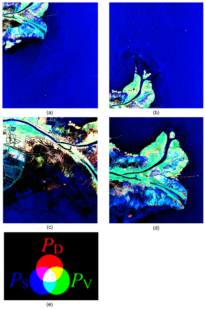
55] used a stacked sparse auto-encoder for multi-layer PolSAR feature extraction. In addition, the input data is represented as a nine-dimensional real vector extracted from the covariance matrix. After polarimetric decomposition, surface scattering, double-bounce scattering, and volume scattering could be acquired [56]. A few studies have implemented these three components in CNNs with overall accuracy (OA) of as high as 95.85% [57]. A few studies have also combined the information in the T matrix and polarization power parameters to classify PolSAR images with different weights. OA was higher by adjusting the weights [58]. Chen et al. [54] improved the performance of a CNN by combining the target scattering mechanism and polarization feature mining. A recent work by He et al. [59] combined the features extracted using nonlinear manifold embedding; next, they applied FCN to input PolSAR images. The final classification was performed using the SVM integration method. In [60], the authors emphasized the computational efficiency of deep learning methods and proposed a lightweight 3D CNN. They demonstrated that the classification accuracy of the proposed method was higher than that of other CNN methods. The number of learning parameters was notably reduced, and high computational efficiency was achieved.
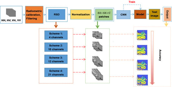
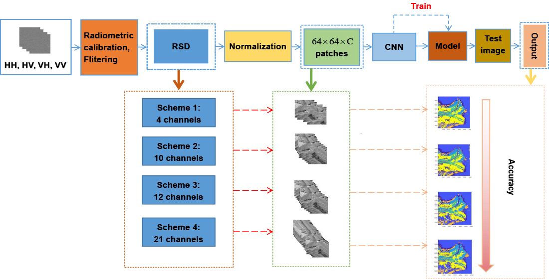
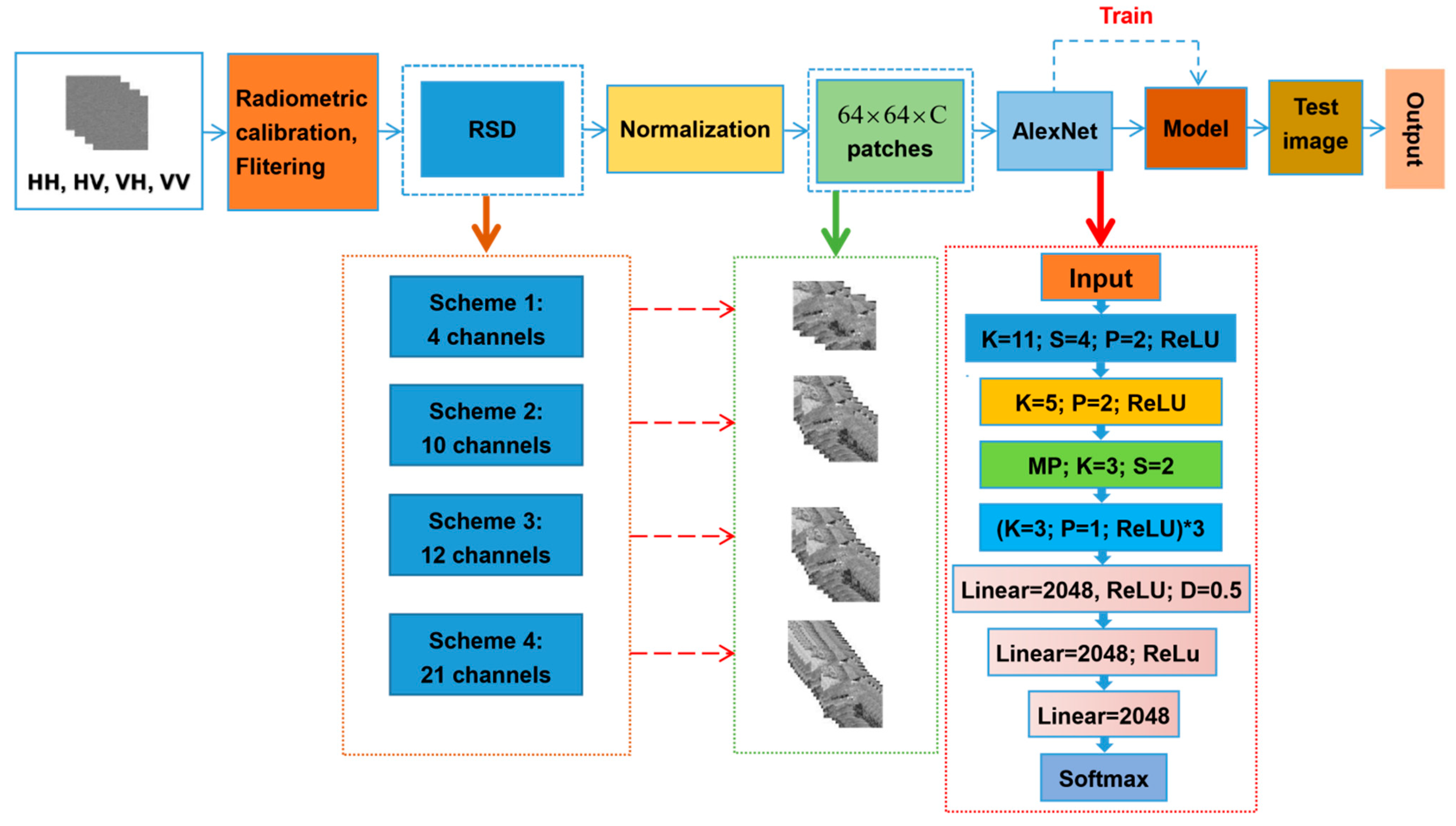
Through the literature survey, we discovered that ground objects could be classified using polarization features decomposed from PolSAR images. However, few studies have focused on polarization scattering features decomposed using excellent polarization decomposition algorithms. Reflection symmetry decomposition (RSD) [61] is an effective algorithm and can be used to obtain polarization scattering characteristics. This study investigated if higher classification accuracy can be acquired when more informative polarimetric features were input CNNs. To this end, this paper proposes four schemes to explore the combination of polarization scattering features for QP image classification based on polarization scattering characteristics obtained through RSD and T matrix. The remainder of this paper is as follows: the first section serves as an introduction to the current research progress of using polarization scattering information and describes the innovations in current; the second section discusses the research area and data preprocessing; the third section discusses the experimental method and the experimental process; the fourth section presents an analysis of the experimental results and accuracy; finally, we discussed the strengths and limitations of the experiment.
The main goals of this study were, therefore, (1) to provide a method for wetlands classification based on polarimetric features; (2) to examine the power of classical CNNs for the classification of back-scattering similar wetland classes; (3) to investigate the generalization capacity of existing CNNs for the classification of different satellite imagery; (4) to explore polarimetric features which are helpful for wetland classification and provide comparisons with different polarimetric features combinations; (5) to compare the performance and efficiency of the most well-known deep CNNs. Thus, this study contributes to the CNN classification tools for complex land cover mapping using QP data based on polarimetric features.

2. Study Area and Data Preprocessing

2.1. Study Area and Data

GF-3 satellite is China’s first C-band high-resolution PolSAR. The satellite has 12 imaging modes, and the spatial resolution ranges from 1 to 500 m. The images obtained by the satellite are broadly used, for example, ship recognition [62], terrain surface classification [63], and feature classification [64]. The quad polarization band 1 (QPSI) imaging mode of the GF-3 satellite has an incidence angle range of 21°–41° and an imaging bandwidth of 20–35 km, which is suitable for researching the Yellow River Delta. Therefore, we selected the QPSI mode of GF-3 to classify ground objects in the Yellow River Delta.
The QP images can be downloaded from the China Ocean Satellite Data Service System [65]. We selected four scenes’ images (14 September 2021 [two images]; 13 October 2021 [one image]; and 12 October 2017 [one image]), the first three images were for training, and the last one was for testing. The imaging mode selected was QPSI and 8 m in spatial resolution. The longitude and latitude ranges were (118°33′–119°20′ E, 37°35′–38°12′ N), and the incidence angle (inc. angle) ranges from 30.97°–37.71°. The images selected for the experiment are specified in Table 1.

2.2. Data Preprocessing

Before inputting the QP images into CNNs, the images should be processed through radiometric calibration, polarization filtering, polarization decomposition, pseudocolor synthesis, data normalization, training dataset making, and so on. The radiometric calibration formula was described in [66].
Owing to the imaging mechanism of PolSAR, speckles are inevitably generated in the images, thereby reducing the accuracy. The non-local mean filtering method proposed by Chen et al. in 2011 can effectively suppress speckles. In the non-local mean filtering method, the neighborhood is considered a single unit [67]. This method not only focused on the similarity between two individual pixels but also the similarity between two pixels. It is more stable and effective than traditional neighborhood filtering methods. Therefore, we adopted non-local mean filtering to despeckle PolSAR images.
The material, size, and shape of the ground objects could influence polarimetric features. The back-scattering coefficients of different targets are different because of characteristics such as shapes. In PolSAR, the back-scattering coefficient of the target is represented by the T matrix. Polarization decomposition theories have been proposed to decompose the scattering matrix into several different components to interpret the scattering mechanism of targets. Polarization characteristics are defined using the parameters extracted from QP data, which can reflect the polarization characteristics of ground objects to a certain extent, for example, total polarization power, scattering angle, and similarity parameters. Polarization features are extensively used for polarization target feature extraction, target classification, target detection, and parameter inversion.
Traditional polarization decomposition can only decompose a small number of polarization features. For example, Freeman decomposition [56] can only save the information of 5 real elements of the original polarization coherence matrix along with loss of polarization information occurring along with the presence of a negative power component in the results. Yamaguchi decomposition [68] can only save six real elements. The de-orientation Freeman decomposition [69] can save six real elements and the de-orientation Yamaguchi decomposition [70] can save seven real elements. Cui decomposition [71] and improved Cui decomposition [72] neither lead to polarization information loss nor have a negative power component. However, the model of their third component is only a polarization coherence matrix with rank 1. Thus, complete polarization decomposition was not achieved using these methods. RSD is a novel algorithm-based non-coherent polarization decomposition method that does not involve any loss of polarization information [61]. The decomposition algorithm is complete and has excellent performance. The three components obtained through decomposition using RSD satisfy the reflection symmetry assumption. RSD can decompose all polarization scattering features and completely reconstruct the polarization coherence matrix according to the decomposed polarization features. RSD is a highly effective polarization decomposition scheme. With RSD, more polarimetric features can be obtained. Therefore, the polarization scattering characteristics used in this study are new. Owing to these advantages, we selected RSD as the polarization decomposition method in this study.
The polarization features obtained after decomposition through RSD included volume scattering value PV, surface scattering value PS, double bounce value PD, the total power value of the second component of RSD P2, the total power value of the third component of RSD P3, twice the orientation angle θ, twice the helix angle φ, power proportion of spherical scattering in the second component of RSD x, power proportion of spherical scattering in the third component of RSD y, the phase a of the second component of RSD, and the phase b of the third component of RSD.
To label the targets on the images conveniently, the obtained polarization scattering parameters are required to be synthesized in pseudo color. We assigned red, green, and blue to PD, PS, and PV, respectively (Figure 1e). The pseudocolor images for training and testing are displayed in Figure 1:
The correspondence of training and validating labels to QP image classification is necessary. We used unmanned aerial vehicle (UAV) images (displayed in Figure 2), combined with empirical knowledge, for marking targets to guarantee the accuracy of the labeled training datasets. Different ground objects were randomly sampled to generate training sets for the CNN. Next, the trained model was used to classify QP images that were not in the training datasets; thus, the training images and testing images of the same scenes were captured at different times.
In this study, we classified seven species according to the survey results: nearshore water, seawater, spartina alterniflora, tamarix, reed, tidal flat, and suaeda salsa; we labeled these targets from number 1 to 7, respectively. We selected 800 samples of each category for training and 200 for validation. The details are shown in Table 2.

3. Method

3.1. Normalized Method

The polarization coherence matrix can be expressed in (1). The reciprocity theorem was satisfied in the PolSAR images.
T = k k H = [ T 11 T 12 T 13 T 12 T 22 T 23 T 13 T 23 T 33 ]
where the superscript * represents conjugation, the superscript H represents conjugate transpose, <•> represents set average, and k is the Pauli vector. The relationship of the elements of the polarization scattering matrix can be expressed in (2).
k = 1 2 [ S HH + S VV S HH S VV S HV S VH ]
The back-scattering coefficients of PolSAR images after RSD are distributed non-linear because of the imaging mechanism of PolSAR. The linear normalization methods (such as maximum and minimum normalization and Z-score standardization) are unsuitable for PolSAR image processing. Therefore, according to the relationship between the total polarization power of PolSAR and each polarization scattering feature, this study adopted different methods to normalize polarimetric features. First, before employing the normalization method for scattered polarization features, the total polarization power span is required to be processed. Span refers to the sum of the diagonal values of the T matrix:
S p a n = T 11 + T 22 + T 33
To better represent Span, it is converted into a quantity in dB:
P 0 = 10 · log 10 ( S p a n )
Several different types of ground objects are distributed in the Yellow River Delta. Understanding the distribution of the total polarization power values of the targets is necessary. To further investigate the distribution of the classified features, we statistically analyzed the features. The experimental results indicated that the ground features were mainly distributed within the range [−30 dB, 0 dB] as well as P0. Therefore, we intercepted [−30 dB, 0 dB] of the scattering characteristics for classification.
The input polarization features should be normalized before training and testing the neural network. Since Span = T11 + T22 + T33 for variables processing in the T matrix, Tij/Span (where i and j represent the row and column numbers of the T matrix) is used to normalize each element in the T matrix. For the complex elements in the non-diagonal elements of the T matrix, the real and imaginary parts are divided by Span to realize normalization.
The following physical quantities have a lower magnitude than the total polarization power Span: volume scattering component power value PV, surface scattering power value PS, double bounce scattering power value PD, the total power value of the second component of RSD P2, and total power value of the third component of RSD P3. Therefore, these parameters were divided by the span value to realize normalization.
The power ratio x of the spherical scattering of the second component of the symmetric decomposition of reflection and the power ratio y of the spherical scattering of the third component of the symmetric decomposition of the reflection was within the range [0, 1]. Thus, these parameters were not required to be normalized.
The range of the double directional and double spiral angles was (-π/2, π/2]. The RSD phase of the second component T12 element a and that of the third component T13 element b were within the range [−π, π]. Therefore, these parameters were processed as follows (5):
X 1 = x m max + n m i n 2 m m a x n m i n 2
X1 is the normalized quantity and x is the quantity to be processed; mmax and nmin are the maximum and minimum values within the range of the physical quantities to be processed.
A few parameters processed using formula (5) were within the range [−1, 1]. To match the value range of the neural network activation function, the range [−1, 1] of the parameters was required to be reduced to [0, 1]. Next, the following formula was used:
z = y + 1 2
where y is the quantity to be processed at range of [−1, 1], z is the quantity after processing within the range [0, 1].

3.2. Schemes

Based on the polarization features generated through RSD and the T matrix, four schemes were proposed. First, we used the polarimetric features in the polarization coherence matrix (T) to classify QP images, which have been extensively reported in the literature [53,54,55,56]. Among them, the three main diagonal elements of T (T11, T22, and T33) contained most of the polarization information. The polarimetric features should be normalized before input to CNNs. The input polarimetric features can be normalized according to the relationship between the elements in the T matrix and Span. Therefore, we considered these four elements as scheme 1.
A substantial amount of polarimetric information was contained in the T matrix. In addition to the three diagonal elements, the non-diagonal elements also include relevant information. All elements of the T matrix and Span were regarded as scheme 2.
In addition to using the information in the T matrix, various polarization power quantities (PS, PD, PV, P2, P3, θ, φ, x, y, a, b and P0) were decomposed using the RSD method. Given that normalization was involved, 12 polarization quantities along with Span were regarded as scheme 3. Finally, a total of 20 polarimetric features and Span were selected as scheme 4. In order well understand, similar to picture processing, a polarimetric feature was regarded as a channel here. The details are displayed in Table 3.

3.3. Exp

CNNs are used to process data with similar network structures. A complete CNN is generally composed of data input layers, convolution layers, activation layers, pooling layers, and full connection layers. CNNs with a certain depth and width can extract deeper features of images and can perform better object recognition and classification. In 2012, Geoffrey Hinton proposed AlexNet [73] which uses ReLU as the nonlinear activation function, dropout was adopted to randomly deactivate a few neurons for the first time which can avoid the overfitting of the model. The model has been applied by many scholars, thus marking the emergence of a new era of deep learning. Only two years later, VGG-Nets [74] were proposed and became a new star among relevant researchers. Both AlexNet and VGG16 are classic models with shallow layers, good generalization performance, and less time-consuming compared with other deeper state-of-art networks. Therefore, these two CNNs were selected as the backbone networks in this study.

3.4. Experiment

The procedure of the experiment is available as follows: First, the PolSAR data should be radiometrically calibrated [66] and filtered [67], a total of 21 polarimetric features were extracted from the RSD [61], and four schemes were proposed. Next, the polarimetric features were normalized before input CNNs [73,74]. Next, image cubes were extracted from training images and then divided into training datasets and validation datasets. We used training and validation datasets for model training. The model parameters are described in [73,74]. We used the weights and other parameters for testing when the model performed well. According to the processing methods, we took AlexNet for example, the experimental flow is displayed in Figure 3. The flow chart can be roughly divided into two lines. The first line is the main part of the experiment, and each color represents different processing content. The second line explains the main processing part of the first line. The orange box is the four research schemes designed, the green box is the visualization of the batch data of the corresponding research scheme, and the red box is the architecture and parameters of AlexNet.
The pseudocodes of the experiment are as follows:
Pseudocodes of the experiment: QP Classification through CNNs Based on Polarimetric Features
Input: GF-3 quad PolSAR images.
Output: classified results.
1: Calibrate GF-3 PolSAR images [66].
2: Nonlocal filtering [67].
3: Polarimetric decomposition [61].
4: Extract polarimetric features.
5: Nonlinear normalization.
6: Four schemes are proposed based on the relationship between the T matrix and span.
7: Extract training datasets: validating datasets = 4:1.
8: Inputting datasets into CNN [73,74].
for i < N do
   the train one time.
If good fitting, then
  Save model, and break.
else if over-fitting or under-fitting, then
  Adjust parameters includes, i.e., learning rate, bias.
end
9.Test images are input to the model, and do predict to the patches of all pixels.
10. Do method evaluation, i.e., Statistic OA and Kappa coefficient.
(N respents the epoches, H presents the image’s height and W presents the image’s width)
Conventional image classification involves feature extraction and classifier design. The quality of the extracted polarimetric features is crucial. Spatial information not only depended on the target itself but also was related to its neighborhoods. Neighborhood data included polarization features and spatial image patterns around the center point, indicating that different channel samples within the same range were input in AlexNet.
The batch size was set at 64 in the experiment reported in [74], Kaiming initialization was also used [75], with the initial learning rate being 0.1, attenuation rate being 0.1, the initial weight being 0.9, and the weight attenuation rate being 0.0005 [8].
When the model fitted well and the validation accuracy improved, the parameters of the model were stored for testing. The unit’s size of training and testing are the same.
We used the cross-entropy loss function, as expressed in (7).
L S o f t m a x = 1 N i L i = 1 N i c = 1 M y i c l o g ( p i c )
where M represents the number of categories, yic is a symbolic function (0 or 1) if the real category of the sample is equal to 1, otherwise 0. The prediction probability of the observation samples is denoted by pic.
After the convolution and pooling layers in CNNs, the feature size could be acquired. Then the full connection and softmax layers were used to distinguish the category of a pixel. We set an empty matrix of the same size as the test image. The predicted label of each pixel was padded into the empty matrix one by one. Finally, the prediction results were output.

3.5. Evaluation Method

A confusion matrix was used to evaluate classification accuracy. A confusion matrix is described in terms of row and column. Evaluation indicators include overall accuracy (OA), mapping accuracy, user accuracy, etc. These accuracy indicators reflect the accuracy of the image classification from different aspects. The confusion matrix was calculated by comparing the position and classification of each measured pixel at the corresponding position and classification of the classified image. Each column of the confusion matrix represented the prediction category; the total number of data points in each column represented the number of data points in this category. Each row represented the appropriate category of data, and the total number of each row represented the number of data instances. The values in each column represented the number of real data points predicted in this category.
The overall accuracy can be expressed as follows:
ρ c = k = 1 n ρ k k ρ
where ρ is the total number of classified pixels and ρkk is the number of correctly classified pixels.
The kappa coefficient was expressed as,
K a p p a = N i = 1 r x i i i = 1 r ( x i + x + i ) N 2 i = 1 r ( x i + x + i )
where r is the total number of columns in the confusion matrix (total number of categories); xii is the number of pixels on row i and column i of the confusion matrix (number of correct classifications); and xi+ and x+i are the total number of pixels in the row and column, respectively; N is the total number of pixels used for accuracy evaluation.

4. Results

We classified the QP image obtained on October 12, 2017, according to the four schemes. We selected 1000 samples of each category and obtained OA and kappa coefficients (K) to evaluate the algorithm performance. According to the above schemes and experiment, the results using the four schemes are displayed in Figure 4. We drew the ground-truth map of the test image according to the investigation, as displayed in Figure 4e.
According to the classification results on AlexNet, the highest OA and kappa coefficient can be obtained when we adopt 21 total polarimetric features. The performance of scheme 2 and scheme 3 is similar but better than scheme 1. In addition, the OA and kappa coefficient of scheme 3 is slightly higher than scheme 2. The confusion matrix is displayed in Table 4.
Based on the confusion matrixes of the four research schemes, we inferred that the more polarimetric features were input AlexNet, the higher OA acquired. When 21 polarimetric features were used for classification, the OA was 96.54%, which was 8.13% higher than that obtained by using only the main diagonal elements of the T matrix, 2.88% higher than that obtained using the matrix and non-diagonal elements, and 1.1% higher than that obtained using polarization power and other polarimetric features. The OA of classification can be improved by using more informative polarimetric features.
Similarly, we conducted experiments on VGG16 as well. The parameters are described in [74] and [8]. The OA of scheme 4 is 94.93%, which is 5.4% higher than just using the three diagonal elements of the T matrix. The performance of scheme 2 and scheme 3 is similar but better than scheme 1. The results indicated that higher OAs and kappa coefficients can be acquired when more informative polarimetric features are input VGG16. The confusion matrix of VGG16 is displayed in Table 5.

5. Discussion

To verify that the polarization features classified by employing CNNs were informative, we designed noise test experiments by adding one, two, and three channels of Gaussian random noise to each scheme. The results on AlexNet indicated that after adding one channel of Gaussian random noise, the OAs of schemes from schemes 1 to 4 were 81.36%, 85.47%, 94.93%, and 95.71%, respectively, and the kappa coefficients were 78.25%, 83.05%, 94.08%, and 95%, respectively. The OAs and kappa coefficients were lower than those obtained using the original schemes. Similarly, upon adding two channels of Gaussian random noise, the OAs using the four schemes were 81.2%, 90.44%, 94.9%, and 93.76%, respectively, and kappa coefficients were 78.07%, 88.85%, 93.22%, and 92.72%, respectively. Upon adding three channels of Gaussian random noise, the OAs of the four schemes were 85.09%, 91.87%, 93.89%, and 94.5%, respectively, and the kappa coefficients were 82.6%, 90.52%, 92.87%, and 93.58%, respectively. When we added noise on VGG16, the OAs and kappa coefficient also decreased to varying degrees. The OAs and kappa coefficients obtained upon adding the noise were worse than the original schemes, meaning that AlexNet and VGG16 had a good anti-noise performance. Higher accuracy can be acquired when adopting more informative polarimetric features to classify QP images. Furthermore, the results of RSD were slightly better than the T matrix.
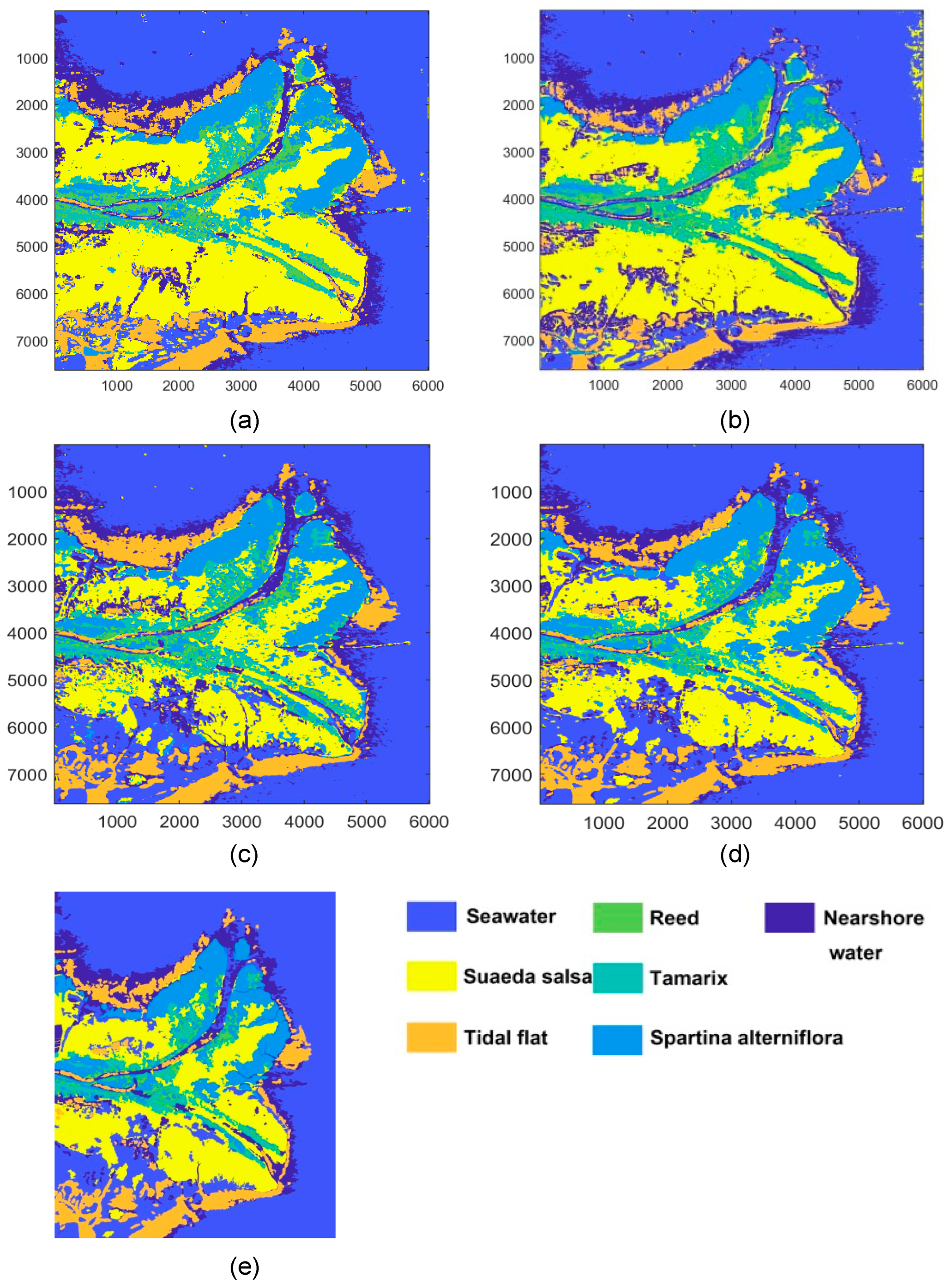
According to the results obtained using different schemes, the scheme with 21 polarimetric features had the highest OA because of more scattering of polarization information. The back-scattering coefficient is a crucial factor affecting the classification of targets. A CNN can distinguish targets easily when the back-scattering coefficients of specific targets differ from those of other ground objects. For example, the back-scattering coefficients of seawater and vegetation are considerably different; thus, the boundary between them is apparent. Distinguishing seawater from nearshore water is challenging because of their similar back-scattering coefficients.

6. Conclusions

In this study, we employed two well-known CNNs to classify QP images of the Yellow River Delta captured during summer. Accordingly, the wetlands in this area were classified as nearshore water, seawater, spartina alterniflora, tamarix, reed, tidal flat, and suaeda salsa.
With the polarimetric features from RSD and T matrix, four schemes were proposed. After radiation correction, polarization filtering, and normalization, the corresponding ground objects of the images were divided into training and validation datasets. The OAs of the classification were up to 96.54% and 94.93% which were 8.13% and 5.4% higher than the T matrix. The OAs of the four schemes were all higher than 88%. The results indicated that the accuracy was improved when more informative polarimetric features were input CNNs. The classification results also confirmed that the CNN classification method accounting for polarimetric features can be applied to QP images of wetlands classification. Furthermore, the back-scattering coefficient is a crucial parameter for distinguishing ground objects. The results obtained through RSD were slightly better than those obtained using the T matrix. Therefore, RSD can help improve the accuracy of polarimetric SAR image classification of wetland objects using CNNs. This study provides a method for wetlands classification based on polarimetric features and will promote future research on wetland cover.
The QP images captured using the GF-3 satellite contain a substantial amount of information with high utilization value. However, there only four summer-time images of the Yellow River Delta captured between 2016 and 2022 are available. These images are insufficient for analyzing the ground cover of the entire Yellow River Delta. Meanwhile, there are no benchmarks for performance assessment. We intend to utilize more GF-3 QP images of the Yellow River Delta in the future to train a model that can be applied to both summer and winter conditions. Furthermore, optical and QP images can be fused to classify wetlands. In addition, we will use novel CNNs or propose algorithms to analyze the Yellow River Delta in future studies.

Author Contributions

W.A. procured GF-3 data; S.Z. processed data, obtained the results, and authored the manuscript; C.X. and W.A. revised the manuscript; S.Z., Y.Z. and L.C. supervised the study; W.A. guided the deep learning model training; L.C. provided some suggestions for this paper. All authors have read and agreed to the published version of the manuscript.

Funding

This study was funded by the National Natural Science Foundation of China (61971152) and the National Major Science and Technology Special Scientific Research Project of China’s High-resolution Earth Observation System (41-Y30F07-9001-20/22).

Institutional Review Board Statement

Not applicable.

Informed Consent Statement

Not applicable.

Data Availability Statement

Data were obtained from China Ocean Satellite Data Service System and are available at https://osdds.nsoas.org.cn/ (accessed on 30 July 2022) with the identity of protocol users.

Acknowledgments

The authors thank the reviewers for their constructive feedback on this article.

Conflicts of Interest

The authors declare no conflict of interest.

Abbreviations

The following abbreviations are used in this manuscript:
QPQuad-polarimetric synthetic aperture radar
CNNsConvolutional neural networks
ROIRegin of interest
SASSynthetic aperture sonar
ViTVision transformer
NASNeural architecture search
DARTSDifferentiable architecture search
DOAJDirectory of open access journals
SGDStochastic gradient descent
FCNFully convolutional network
CV-SDFCNComplex-valued domain stacked-dilated convolution
RSDReflection symmetry decomposition
OAOverall accuracy
SARSynthetic aperture radar
SVMSupport vector machine
GANGenerative adversarial network
NBNaive Bayes
RFRandom forest
MLPMultilayer perceptron
SSVITSpatial-spectral vision transformer
PolSARPolarimetric synthetic aperture radar
DEMDigital elevation model
DBNDeep belief network
SAEStack autoencoder
DCAEDeep convolution autoencoder
DSCNNDeep supervised contraction neural network
QPSIQuad polarization band 1
UAVUnmanned aerial vehicle

References

  1. Baolei, Z.; Qiaoyun, Z.; Chaoyang, F.; Qingyu, F.; Shumin, Z. Understanding land use and land cover dynamics from 1976 to 2014 in yellow river delta. Land 2017, 6, 1–20. [Google Scholar]
  2. Touzi, R.; Deschamps, A.; Rother, G. Scattering type phase for wetland classification using C-band polarimetric SAR. In Proceedings of the IGARSS 2008—2008 IEEE International Geoscience and Remote Sensing Symposium, Boston, MA, USA, 7–11 July 2008; Institute of Electrical and Electronics Engineers: Piscataway, NJ, USA, 2008; pp. II-285–II-288. [Google Scholar] [CrossRef]
  3. Chen, Y.; He, X.; Wang, J.; Xiao, R. The Influence of Polarimetric Parameters and an Object-Based Approach on Land Cover Classification in Coastal Wetlands. Remote Sens. 2014, 6, 12575–12592. [Google Scholar] [CrossRef] [Green Version]
  4. Yang, J.; Ren, G.; Ma, Y.; Fan, Y. Coastal wetland classification based on high resolution SAR and optical image fusion. In Proceedings of the 2016 IEEE International Geoscience and Remote Sensing Symposium (IGARSS), Beijing, China, 10–15 July 2016; Institute of Electrical and Electronics Engineers: Piscataway, NJ, USA, 2016; pp. 886–889. [Google Scholar] [CrossRef]
  5. He, Z.; He, D.; Mei, X.; Hu, S. Wetland Classification Based on a New Efficient Generative Adversarial Network and Jilin-1 Satellite Image. Remote Sens. 2019, 11, 2455. [Google Scholar] [CrossRef] [Green Version]
  6. Liu, J.; Li, P.; Tu, C.; Wang, H.; Zhou, Z.; Feng, Z.; Shen, F.; Li, Z. Spatiotemporal Change Detection of Coastal Wetlands Using Multi-Band SAR Coherence and Synergetic Classification. Remote Sens. 2022, 14, 2610. [Google Scholar] [CrossRef]
  7. Gao, Y.; Song, X.; Li, W.; Wang, J.; He, J.; Jiang, X.; Feng, Y. Fusion Classification of HSI and MSI Using a Spatial-Spectral Vision Transformer for Wetland Biodiversity Estimation. Remote Sens. 2022, 14, 850. [Google Scholar] [CrossRef]
  8. Gao, Y.; Li, W.; Zhang, M.; Wang, J.; Sun, W.; Tao, R.; Du, Q. Hyperspectral and multispectral classification for coastal wetland using depthwise feature interaction network. IEEE Trans. Geosci. Remote Sens. 2021, 60, 1–15. [Google Scholar] [CrossRef]
  9. Chen, Y.; He, X.; Xu, J.; Zhang, R.; Lu, Y. Scattering Feature Set Optimization and Polarimetric SAR Classification Using Object-Oriented RF-SFS Algorithm in Coastal Wetlands. Remote Sens. 2020, 12, 407. [Google Scholar] [CrossRef] [Green Version]
  10. DeLancey, E.R.; Simms, J.F.; Mahdianpari, M.; Brisco, B.; Mahoney, C.; Kariyeva, J. Comparing Deep Learning and Shallow Learning for Large-Scale Wetland Classification in Alberta, Canada. Remote Sens. 2020, 12, 2. [Google Scholar] [CrossRef] [Green Version]
  11. Banks, S.; White, L.; Behnamian, A.; Chen, Z.; Montpetit, B.; Brisco, B.; Pasher, J.; Duffe, J. Wetland Classification with Multi-Angle/Temporal SAR Using Random Forests. Remote Sens. 2019, 11, 670. [Google Scholar] [CrossRef]
  12. Faizabadi, A.R.; Zaki, H.F.B.M.; Abidin, Z.B.Z.; Hashim, N.N.W.N.; Husman, M.A.B. Efficient Region of Interest Based Metric Learning for Effective Open World Deep Face Recognition Applications. IEEE Access 2022, 10, 76168–76184. [Google Scholar] [CrossRef]
  13. Yang, M.; Kong, B.; Dang, R.; Yan, X. Classifying urban functional regions by integrating buildings and points-of-interest using a stacking ensemble method. Int. J. Appl. Earth Obs. Geoinf. 2022, 108, 102753. [Google Scholar] [CrossRef]
  14. Feng, J.; Zhang, S.-W.; Chen, L.; Zuo, C. Detection of Alzheimer’s disease using features of brain region-of-interest-based individual network constructed with the sMRI image. Comput. Med Imaging Graph. 2022, 98, 102057. [Google Scholar] [CrossRef] [PubMed]
  15. Ullah, B.; Khan, A.; Fahad, M.; Alam, M.; Noor, A.; Saleem, U.; Kamran, A.M. A Novel Approach to Enhance Dual-Energy X-Ray Images Using Region of Interest and Discrete Wavelet Transform. J. Inf. Processing Syst. 2022, 18, 319–331. [Google Scholar] [CrossRef]
  16. Steiniger, Y.; Kraus, D.; Meisen, T. Survey on deep learning based computer vision for sonar imagery. Eng. Appl. Artif. Intell. 2022, 114, 105157. [Google Scholar] [CrossRef]
  17. Yutong, G.; Khishe, M.; Mohammadi, M.; Rashidi, S.; Nateri, M.S. Evolving Deep Convolutional Neural Networks by Extreme Learning Machine and Fuzzy Slime Mould Optimizer for Real-Time Sonar Image Recognition. Int. J. Fuzzy Syst. 2022, 24, 1371–1389. [Google Scholar] [CrossRef]
  18. Fernandes, J.d.C.V.; de Moura, N.N., Jr.; de Seixas, J.M. Deep Learning Models for Passive Sonar Signal Classification of Military Data. Remote Sens. 2022, 14, 2648. [Google Scholar] [CrossRef]
  19. Gerg, I.D.; Monga, V. Structural Prior Driven Regularized Deep Learning for Sonar Image Classification. In IEEE Transactions on Geoscience and Remote Sensing; Institute of Electrical and Electronics Engineers: Piscataway, NJ, USA, 2022; Volume 60, pp. 1–16. [Google Scholar] [CrossRef]
  20. Varga, D. No-Reference Image Quality Assessment with Convolutional Neural Networks and Decision Fusion. Appl. Sci. 2022, 12, 101. [Google Scholar] [CrossRef]
  21. Pardamean, B.; Cenggoro, T.W.; Rahutomo, R.; Budiarto, A.; Karuppiah, E.K. Transfer learning from chest x-ray pre-trained convolutional neural network for learning mammogram data—Sciencedirect. Procedia Comput. Sci. 2018, 135, 400–407. [Google Scholar] [CrossRef]
  22. Khan, H.A.; Wu, J.; Mushtaq, M.; Mushtaq, M.U. Brain tumor classification in mri image using convolutional neural network. Math. Biosci. Eng. 2020, 17, 6203–6216. [Google Scholar] [CrossRef] [PubMed]
  23. Wang, H.; Xing, C.; Yin, J.; Yang, J. Land Cover Classification for Polarimetric SAR Images Based on Vision Transformer. Remote Sens. 2022, 14, 4656. [Google Scholar] [CrossRef]
  24. Dong, H.; Zou, B.; Zhang, L.; Zhang, S. Automatic Design of CNNs via Differentiable Neural Architecture Search for PolSAR Image Classification. In IEEE Transactions on Geoscience and Remote Sensing; Institute of Electrical and Electronics Engineers: Piscataway, NJ, USA, 2020; Volume 58, pp. 6362–6375. [Google Scholar] [CrossRef] [Green Version]
  25. Dong, H.; Zhang, L.; Zou, B. Exploring Vision Transformers for Polarimetric SAR Image Classification. In IEEE Transactions on Geoscience and Remote Sensing; Institute of Electrical and Electronics Engineers: Piscataway, NJ, USA, 2022; Volume 60, pp. 1–15. [Google Scholar] [CrossRef]
  26. Nie, W.; Huang, K.; Yang, J.; Li, P. A Deep Reinforcement Learning-Based Framework for PolSAR Imagery Classification. In IEEE Transactions on Geoscience and Remote Sensing; Institute of Electrical and Electronics Engineers: Piscataway, NJ, USA, 2022; Volume 60, pp. 1–15. [Google Scholar] [CrossRef]
  27. Xie, W.; Jiao, L.; Hua, W. Complex-Valued Multi-Scale Fully Convolutional Network with Stacked-Dilated Convolution for PolSAR Image Classification. Remote Sens. 2022, 14, 3737. [Google Scholar] [CrossRef]
  28. Moreira, A.; Prats-Iraola, P.; Younis, M.; Krieger, G.; Hajnsek, I. A tutorial on synthetic aperture radar. Geosci. Remote Sens. Mag. IEEE 2013, 1, 6–43. [Google Scholar] [CrossRef] [Green Version]
  29. He, C.; Li, S.; Liao, Z.; Liao, M. Texture Classification of PolSAR Data Based on Sparse Coding of Wavelet Polarization Textons. IEEE Trans. Geosci. Remote Sens. 2013, 51, 4576–4590. [Google Scholar] [CrossRef]
  30. Parikh, H.; Patel, S.; Patel, V. Classification of SAR and PolSAR images using deep learning: A review. Int. J. Image Data Fusion 2019, 11, 1–32. [Google Scholar] [CrossRef]
  31. Yamagata, Y.; Yasuoka, Y. Classification of wetland vegetation by texture analysis methods using ERS-1 and JERS-1 images. In Proceedings of the IEEE International Geoscience & Remote Sensing Symposium, Tokyo, Japan, 18–21 August 1993. [Google Scholar]
  32. Hong, S.H.; Kim, H.O.; Wdowinski, S.; Feliciano, E. Evaluation of polarimetric SAR decomposition for classifying wetland vegetation types. Remote Sens. 2015, 7, 8563–8585. [Google Scholar] [CrossRef]
  33. Ball, J.E.; Anderson, D.T.; Chan, C.S. Comprehensive Survey of Deep Learning in Remote Sensing: Theories, Tools, and Challenges for the Community. J. Appl. Remote Sens. 2017, 11, 042609. [Google Scholar] [CrossRef] [Green Version]
  34. Hinton, G.E.; Osindero, S.; Teh, Y.-W. A Fast Learning Algorithm for Deep Belief Nets. Neural Comput. 2006, 18, 1527–1554. [Google Scholar] [CrossRef] [PubMed]
  35. Vincent, P.; Larochelle, H.; Lajoie, I.; Bengio, Y.; Manzagol, P.-A. Stacked Denoising Autoencoders: Learning Useful Representations in a Deep Network with a Local Denoising Criterion. J. Mach. Learn. Res. 2010, 11, 3371–3408. [Google Scholar]
  36. Krizhevsky, A.; Sutskever, I.; Hinton, G.E. ImageNet Classification with Deep Convolutional Neural Networks. In Proceedings of the 25th International Conference on Neural Information Processing Systems, Lake Tahoe, NV, USA, 3–6 December 2012; pp. 1097–1105. [Google Scholar]
  37. Szegedy, C.; Liu, W.; Jia, Y.; Sermanet, P.; Reed, S.; Anguelov, D.; Erhan, D.; Vanhoucke, V.; Rabinovich, A. Going Deeper with Convolutions. In Proceedings of the IEEE Conference on Computer Vision and Pattern Recognition (CVPR), Boston, MA, USA, 7–12 June 2015. [Google Scholar]
  38. Zhong, P.; Wang, R. Learning Conditional Random Fields for Classification of Hyperspectral Images. IEEE Trans. Image Process 2010, 19, 1890–1907. [Google Scholar] [CrossRef] [PubMed]
  39. Marmanis, D.; Schindler, K.; Wegner, J.D.; Galliani, S.; Datcu, M.; Stilla, U. Classification with an Edge: Improving Semantic Image Segmentation with Boundary Detection. ISPRS J. Photogramm. Remote Sens. 2018, 135, 158–172. [Google Scholar] [CrossRef] [Green Version]
  40. Chen, X.; Xiang, S.; Liu, C.-L.; Pan, C.-H. Vehicle Detection in Satellite Images by Hybrid Deep Convolutional Neural Networks. IEEE Geosci. Remote Sens. Lett. 2014, 11, 1797–1801. [Google Scholar] [CrossRef]
  41. Ghedira, H.; Bernier, M.; Ouarda, T.B.M.J. Application of neural networks for wetland classification in RADARSAT SAR imagery. In Proceedings of the IEEE International Geoscience and Remote Sensing Symposium, Honolulu, HI, USA, 24–28 July 2000. [Google Scholar]
  42. Hänsch, R.; Hellwich, O. Classification of polarimetric SAR data by complex valued neural networks. In Proceedings of the ISPRS Workshop High-Resolution Earth Imaging for Geospatial Information, Hannover, Germany, 2–5 June 2009. [Google Scholar]
  43. Tison, C.; Nicolas, J.M.; Tupin, F.; Maitre, H. A new statistical model for Markovian classification of urban areas in high-resolution SAR images. IEEE Trans. Geosci. Remote Sens. 2004, 42, 2046–2057. [Google Scholar] [CrossRef]
  44. Bentes, C.; Velotto, D.; Lehner, S. Target classification in oceanographic SAR images with deep neural networks: Architecture and initial results. In Proceedings of the 2015 IEEE International Geoscience and Remote Sensing Symposium (IGARSS), Milan, Italy, 26–31 July 2015. [Google Scholar]
  45. Geng, J.; Fan, J.; Wang, H.; Ma, X.; Li, B.; Chen, F. High-Resolution SAR Image Classification via Deep Convolutional Autoencoders. IEEE Geosci. Remote Sens. Lett. 2015, 12, 2351–2355. [Google Scholar] [CrossRef]
  46. Jie, G.; Wang, H.; Fan, J.; Ma, X. Deep Supervised and Contractive Neural Network for SAR Image Classification. IEEE Trans. Geosci. Remote Sens. 2017, 55, 2442–2459. [Google Scholar]
  47. Zhang, L.; Ma, W.; Zhang, D. Stacked sparse autoencoder in PolSAR data classification using local spatial information. IEEE Geosci. Remote Sens. Lett. 2016, 13, 1359–1363. [Google Scholar] [CrossRef]
  48. Hou, B.; Kou, H.; Jiao, L. Classification of Polarimetric SAR Images Using Multilayer Autoencoders and Superpixels. IEEE J. Sel. Top. Appl. Earth Obs. Remote Sens. 2017, 9, 3072–3081. [Google Scholar] [CrossRef]
  49. Zhao, Z.; Jiao, L.; Zhao, J.; Gu, J.; Zhao, J. Discriminant deep belief network for high-resolution SAR image classification. Pattern Recognit. 2017, 61, 686–701. [Google Scholar] [CrossRef]
  50. Gao, F.; Huang, T.; Wang, J.; Sun, J.; Hussain, A.; Yang, E. Dual-branch deep convolution neural network for polarimetric SAR image classification. Appl. Sci. 2017, 7, 447. [Google Scholar] [CrossRef] [Green Version]
  51. Wang, Y.; He, C.; Liu, X.; Liao, M. A Hierarchical Fully Convolutional Network Integrated with Sparse and Low-Rank Subspace Representations for PolSAR Imagery Classification. Remote Sens. 2018, 10, 342. [Google Scholar] [CrossRef] [Green Version]
  52. Qin, F.; Guo, J.; Sun, W. Object-oriented ensemble classification for polarimetric SAR Imagery using restricted Boltzmann machines. Remote Sens. Lett. 2016, 8, 204–213. [Google Scholar] [CrossRef]
  53. Zhou, Y.; Wang, H.; Xu, F.; Jin, Y.Q. Polarimetric SAR image classification using deep convolutional neural networks. IEEE Geosci. Remote Sens. Lett. 2017, 13, 1935–1939. [Google Scholar] [CrossRef]
  54. Chen, S.W.; Tao, C.S. PolSAR image classification using polarimetric-feature-driven deep convolutional neural network. IEEE Geosci. Remote Sens. Lett. 2018, 15, 627–631. [Google Scholar] [CrossRef]
  55. Xie, H.; Wang, S.; Liu, K.; Lin, S.; Hou, B. Multilayer feature learning for polarimetric synthetic radar data classification. In Proceedings of the IGARSS 2014—2014 IEEE International Geoscience and Remote Sensing Symposium, Quebec City, QC, Canada, 13–18 July 2014. [Google Scholar]
  56. Freeman, A.; Durden, S.L. A three-component scattering model for polarimetric SAR. IEEE Trans. Geosci. Remote Sens. 1998, 36, 963–973. [Google Scholar] [CrossRef] [Green Version]
  57. Zhang, J.; Zhang, W.; Hu, Y.; Chu, Q.; Liu, L. An improved sea ice classification algorithm with Gaofen-3 dual-polarization SAR data based on deep convolutional neural networks. Remote Sens. 2022, 14, 906. [Google Scholar] [CrossRef]
  58. Chen, B.; Wang, S.; Jiao, L.; Stolkin, R.; Liu, H. A three-component fisher-based feature weighting method for supervised PolSAR image classification. IEEE Geosci. Remote Sens. Lett. 2014, 12, 731–735. [Google Scholar] [CrossRef]
  59. He, C.; Tu, M.; Xiong, D.; Liao, M. Nonlinear manifold learning integrated with fully convolutional networks for PolSAR image classification. Remote Sens. 2020, 12, 655. [Google Scholar] [CrossRef] [Green Version]
  60. Dong, H.; Zhang, L.; Zou, A. PolSAR Image Classification with Lightweight 3D Convolutional Networks. Remote Sens. 2020, 12, 396. [Google Scholar] [CrossRef]
  61. An, W.T.; Lin, M.S. A reflection symmetry approximation of multi-look polarimetric SAR data and its application to freeman-durden decomposition. IEEE Trans. Geosci. Remote Sens. 2019, 57, 3649–3660. [Google Scholar] [CrossRef]
  62. Bentes, C.; Velotto, D.; Tings, B. Ship classification in TerraSAR-X images with convolutional neural networks. IEEE J. Ocean. Eng. 2018, 43, 258–266. [Google Scholar] [CrossRef] [Green Version]
  63. Sunaga, Y.; Natsuaki, R.; Hirose, A. Land form classification and similar land-shape discovery by using complex-valued convolutional neural networks. IEEE Trans. Geosci. Remote Sens. 2019, 57, 7907–7917. [Google Scholar] [CrossRef]
  64. Hou, X.; Wei, A.; Song, Q.; Lai, J.; Wang, H.; Xu, F. FUSAR-Ship: Building a high-resolution SAR-AIS matchup dataset of Gaofen-3 for ship detection and recognition. Sci. China Inf. Sci. 2020, 63, 140303. [Google Scholar] [CrossRef] [Green Version]
  65. China Ocean Satellite Data Service System. Available online: https://osdds.nsoas.org.cn/ (accessed on 5 October 2022).
  66. User Manual of Gaofen-3 Satellite Products. China Resources Satellite Application Center: Hong Kong, China, 2016.
  67. Chen, J.; Chen, Y.L.; An, W.T.; Cui, Y.; Yang, J. Nonlocal filtering for polarimetric SAR data: A pretest approach. IEEE Trans. Geosci. Remote Sens. 2011, 49, 1744–1754. [Google Scholar] [CrossRef]
  68. Yamaguchi, Y.; Moriyama, T.; Ishido, M.; Yamada, H. Four-component scattering model for polarimetric SAR image decomposition. IEEE Trans. Geosci. Remote Sens. 2005, 43, 1699–1706. [Google Scholar] [CrossRef]
  69. An, W.; Cui, Y.; Yang, J. Three-Component Model-Based Decomposition for Polarimetric SAR data. IEEE Trans. Geosci. Remote Sens. 2010, 48, 2732–2739. [Google Scholar]
  70. Yamaguchi, Y.; Sato, A.; Boerner, W.M.; Sato, R.; Yamada, H. Four-component scattering power decomposition with rotation of coherency matrix. IEEE Trans. Geosci. Remote Sens. 2011, 49, 2251–2258. [Google Scholar] [CrossRef]
  71. Cui, Y.; Yamaguchi, Y.; Yang, J.; Kobayashi, H.; Park, S.; Singh, G. On Complete Model-Based Decomposition of Polarimetric SAR Coherency Matrix Data. IEEE Trans. Geosci. Remote Sens. 2014, 52, 1991–2001. [Google Scholar] [CrossRef]
  72. An, W.; Xie, C. An Improvement on the Complete Model-Based Decomposition of Polarimetric SAR Data. IEEE Geosci. Remote Sens. Lett. 2014, 11, 1926–1930. [Google Scholar]
  73. Krizhevsky, A.; Sutskever, I.; Hinton, G. ImageNet classification with deep convolutional neural networks. Adv. Neural Inf. Process. Syst. 2017, 60, 84–90. [Google Scholar] [CrossRef] [Green Version]
  74. Simonyan, K.; Zisserman, A. Very deep convolutional networks for large-scale image recognition. Comput. Sci. 2014, 60, 84–90. [Google Scholar]
  75. He, K.; Zhang, X.; Ren, S.; Sun, J. Delving deep into rectifiers: Surpassing human-level performance on imagenet classification. In Proceedings of the 2015 IEEE International Conference on Computer Vision, Santiago, Chile, 7–13 December 2015. [Google Scholar]
Figure 1. Pseudocolor images. (a)Training image 1, (b) Training image 2, (c) Training image 3, (d)Testing image, (e) A schematic of the classical coloring scheme of polarization decomposition using pseudo color synthesis.
Remotesensing 14 05133 g001
Figure 2. UAV images of ground objects. (a) Nearshore water, (b) Seawater, (c) Spartina alterniflora, (d) Suaeda salsa, (e) Tamarix, (f) Reed, (g) Tidal flat.
Remotesensing 14 05133 g002
Figure 3. Experimental flow on AlexNet (where C presents channels, K represents kernel size, S presents stride, P represents padding, MP represents max pooling).
Remotesensing 14 05133 g003
Figure 4. Results on AlexNet. (a) 4channels result, (b) 10 channels result, (c) 12 channels result, (d) 21 channels result, (e) Ground-truth map.
Remotesensing 14 05133 g004
Table 1. Experiment images.
IdDateTime (UTC)Inc. Angle (°)ModeResolutionUse
12021-09-1422:14:1130.98QPSI8 mTrain
22021-09-1422:14:0630.97QPSI8 mTrain
32021-10-1310:05:3537.71QPSI8 mTrain
42017-10-1222:07:3636.89QPSI8 mTest
Table 2. Samples distribution.
ImagesNearshore WaterSeawaterSpartina AlternifloraTamarixReedTidal FlatSuaeda Salsa
20210914_15004001000500500500500
20210914_25002000005000
20211013040005005000500
Total1000100010001000100010001000
Table 3. Four schemes.
IDChannelsPolarimetric Parameters
14T11, T22, T33, P0
210T11, T22, T33, Re(T12), Re(T13), Re(T23), Im(T12), Im(T13), Im(T23), P0
312PS, PD, PV, P2, P3, θ, φ, x, y, a, b, P0
421T11, T22, T33, Re(T12), Re(T13), Re(T23), Im(T12), Im(T13), Im(T23), PS, PD, PV, P2, P3, θ, φ, x, y, a, b, P0
Table 4. Confusion matrixes of the four schemes on AlexNet.
IDGround-ObjectsNearshore WaterSeawaterSpartina AlternifloraTamarixReedTidal FlatSuaeda SalsaAcc (%)OA (%)K
4Nearshore water8981000101089.988.410.88
Seawater169820000298.2
Spartina alterniflora00782631530278.2
Tamarix000947530094.7
Reed0033406660066.6
Tidal flat3424000942094.2
Suaeda salsa002800097297.2
10Nearshore water964700029096.493.660.93
Seawater129870000198.7
Spartina alterniflora0095530120395.5
Tamarix000960400096
Reed00089920099.2
Tidal flat72212000716071.6
Suaeda salsa120600098298.2
12Nearshore water 7960000204079.695.440.95
Seawater69930001099.3
Spartina alterniflora009663120196.6
Tamarix00099820099.8
Reed002499670096.7
Tidal flat11000998099.8
Suaeda salsa1602100096396.36
21Nearshore water 921600011092.196.540.97
Seawater99940001099.4
Spartina alterniflora009650002796.5
Tamarix0028949320094.9
Reed007299680096.8
Tidal flat700000988098.8
Suaeda salsa000220097397.3
Table 5. Confusion matrixes of the four schemes on VGG16.
IDGround-ObjectsNearshore WaterSeawaterSpartina AlternifloraTamarixReedTidal FlatSuaeda SalsaAcc (%)OA (%)K
4Nearshore water 8913900070089.189.530.88
Seawater59920000399.2
Spartina alterniflora0086146930086.1
Tamarix000963370096.3
Reed006209380093.8
Tidal flat33726200635063.5
Suaeda salsa001300098798.70
10Nearshore water8897400037088.992.060.91
Seawater79910000299.1
Spartina alterniflora70993000099.3
Tamarix000979210097.5
Reed007309270092.7
Tidal flat70257000670367
Suaeda salsa001100098998.9
12Nearshore water 86825000107086.892.210.91
Seawater59950000099.5
Spartina alterniflora009643600096.4
Tamarix002066480014664.8
Reed00069940099.4
Tidal flat121000987098.7
Suaeda salsa00100099999.9
21Nearshore water 9221000068092.294.930.94
Seawater59931001099.3
Spartina alterniflora009683200096.8
Tamarix00128461420084.6
Reed007299680096.8
Tidal flat700000988098.8
Suaeda salsa000220097397.3
Publisher’s Note: MDPI stays neutral with regard to jurisdictional claims in published maps and institutional affiliations.

