
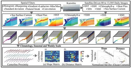
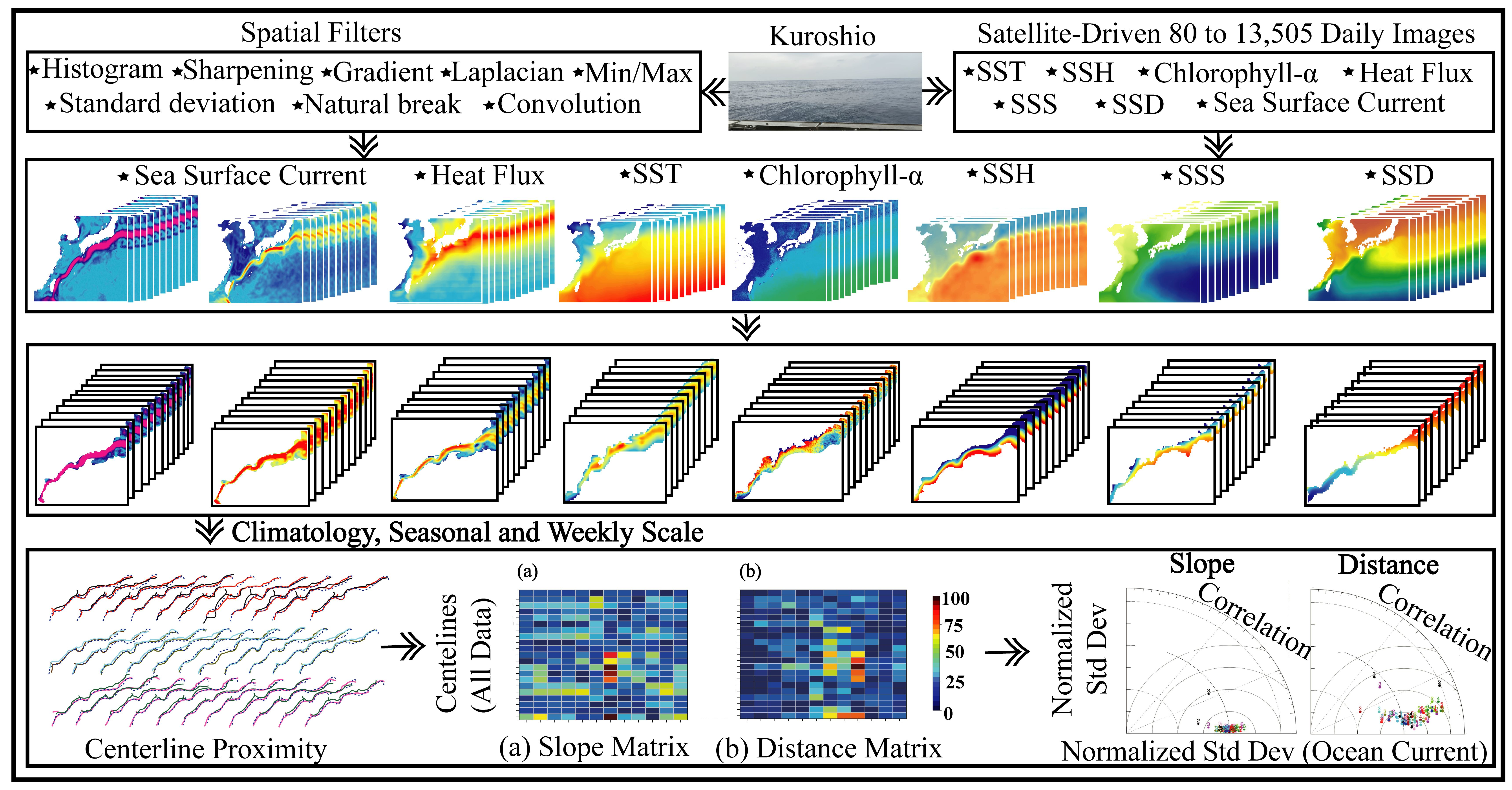
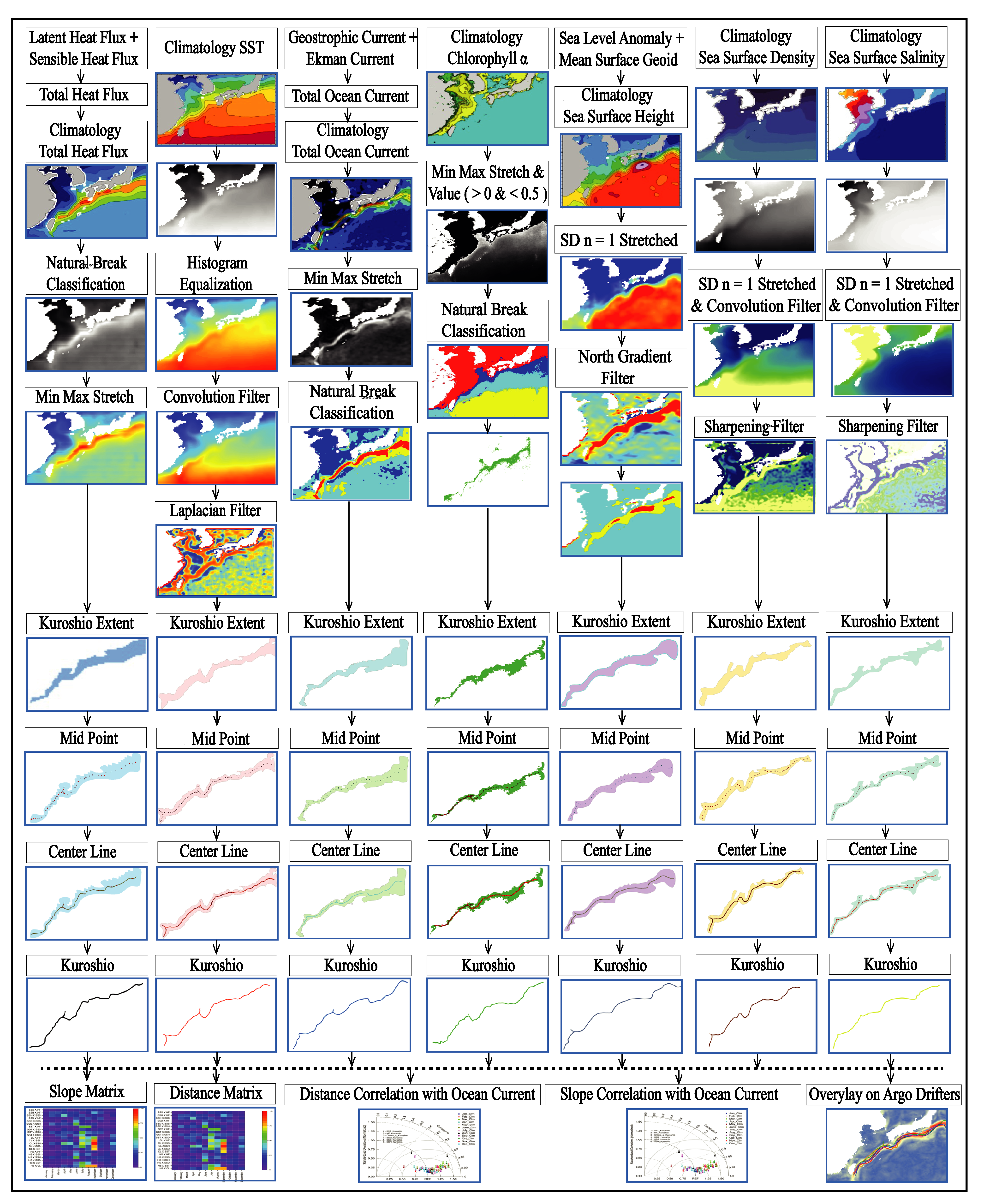
A Combination of Spatial Domain Filters to Detect Surface Ocean Current from Multi-Sensor Remote Sensing Data


Abstract
:
1. Introduction
2. Data and Methods
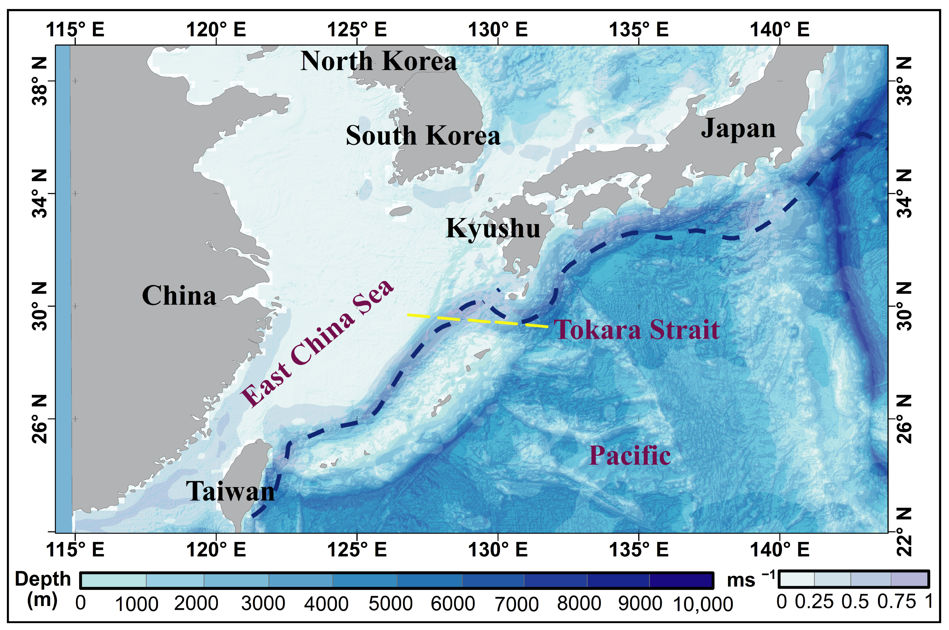
2.1. Study Area
2.2. Data
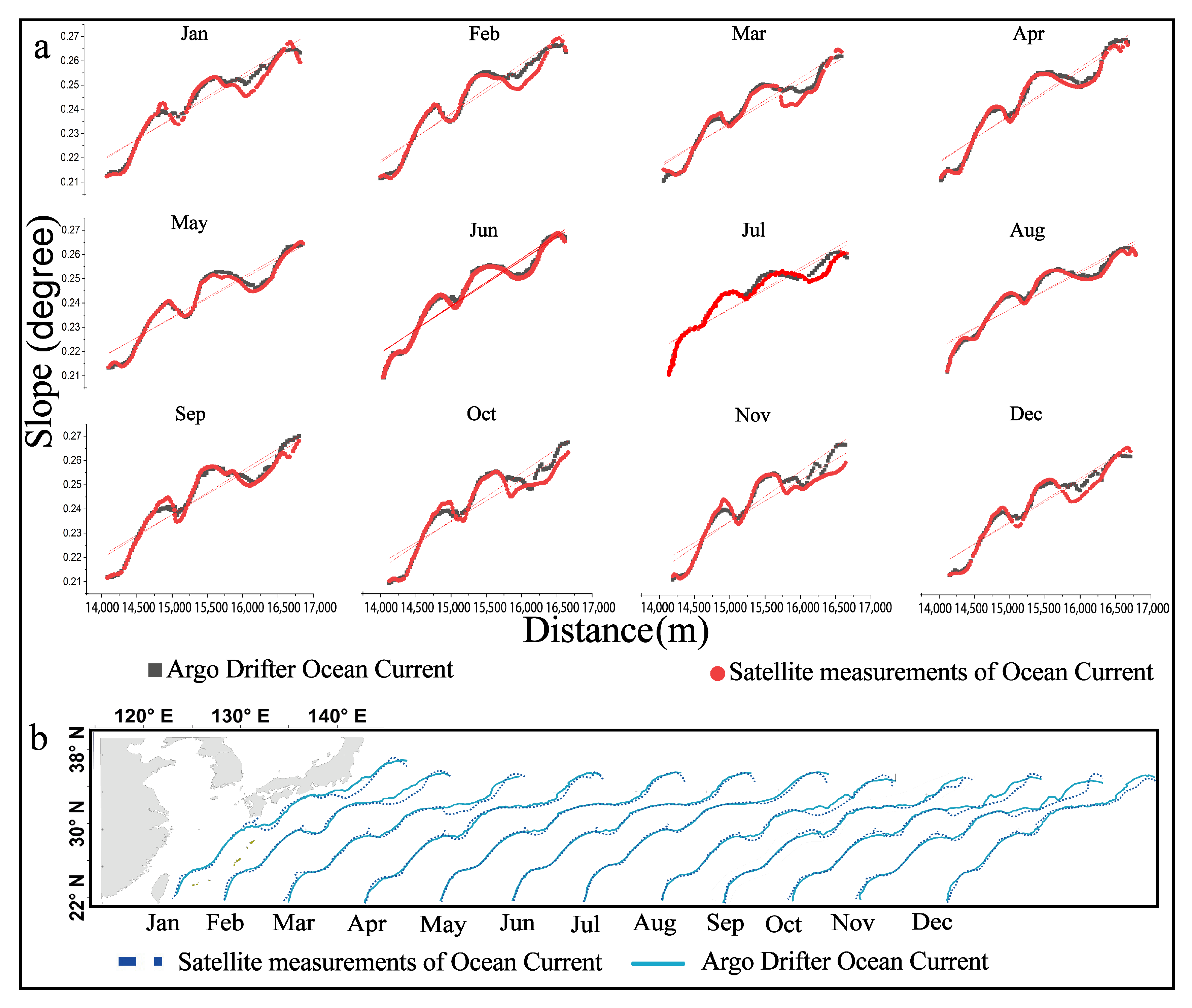
2.2.1. Lagrangian Argo Drifter Data
2.2.2. Sea Surface Currents
2.2.3. SST
- In-Situ and drifter data transformed to traditional alphanumeric codes combined with the universal binary data format.
- Obtaining SST also from Argo floats.
- The satellite input is modernized to operational meteorological satellites A and B.
- Revised ship-based buoy SST rectification method and sea-ice-concentration to SST.
2.2.4. Heat Flux
- A comprehensive data set from research vessels and drifters for validation.
- Satellite and in-situ data are collected over a region of 200 km approximately around each point of situ.
- Issued involving diurnal cycles are resolved using skin SST from refined high-resolution data.
- Betterment of models to calculate bulk turbulent flux.
- Surface air temperature and humidity retrieval from satellites.
- Sea flux products are calibrated by applying the end products to physical phenomena, for instance, heat transport in the atmosphere and ocean.
2.2.5. Chlorophyll-
2.2.6. SSH
2.2.7. SSS and SSD
2.3. Methods
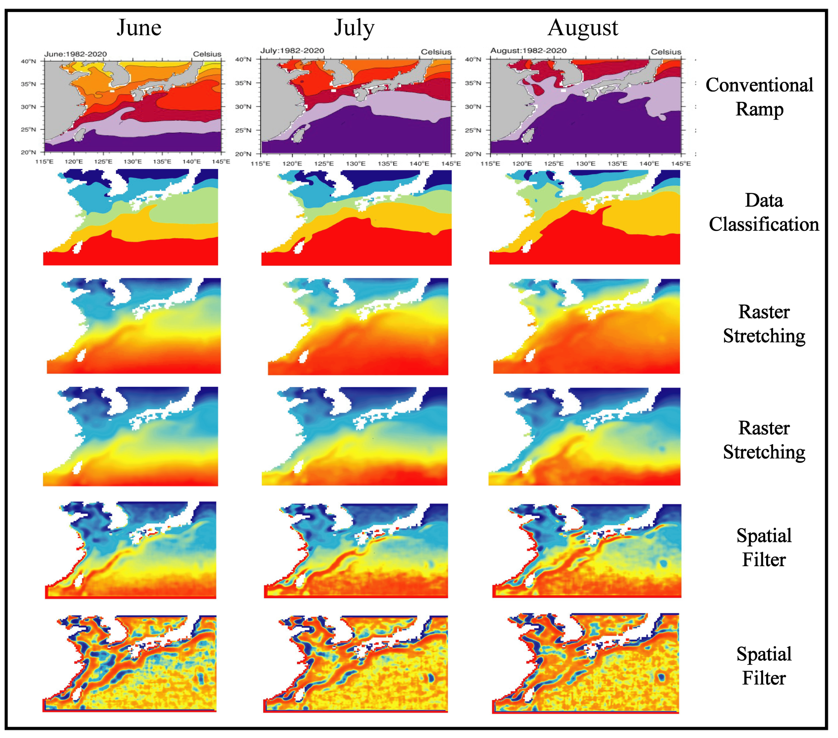
2.3.1. Raster Filters
Convolution Filter
Laplacian Filter
Sharpening Filter
2.3.2. Gradient Computation
2.3.3. Conditional Filtering
- = Enhanced output image.
- = Input images after applying improvised range of chlorophyll-.
- , = Minimum and maximum intensity values of input image.
- N = Total number of intensity values assigned to a pixel.
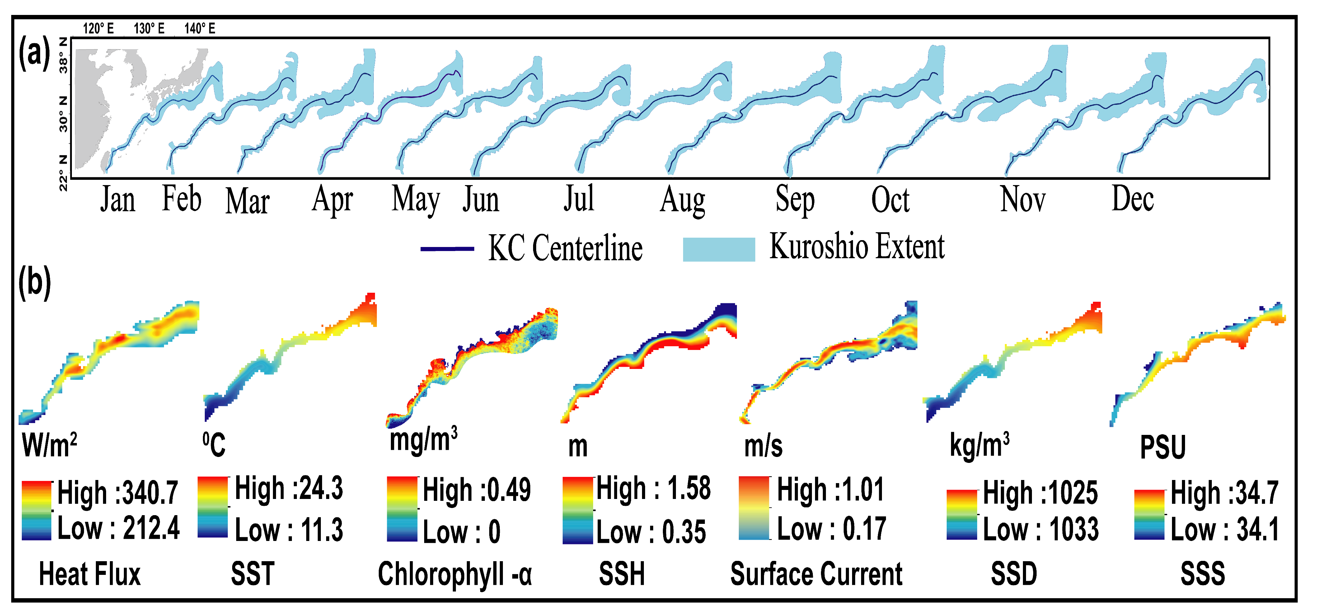
2.3.4. Classification Method to Represent Kuroshio
2.3.5. Feature Extraction
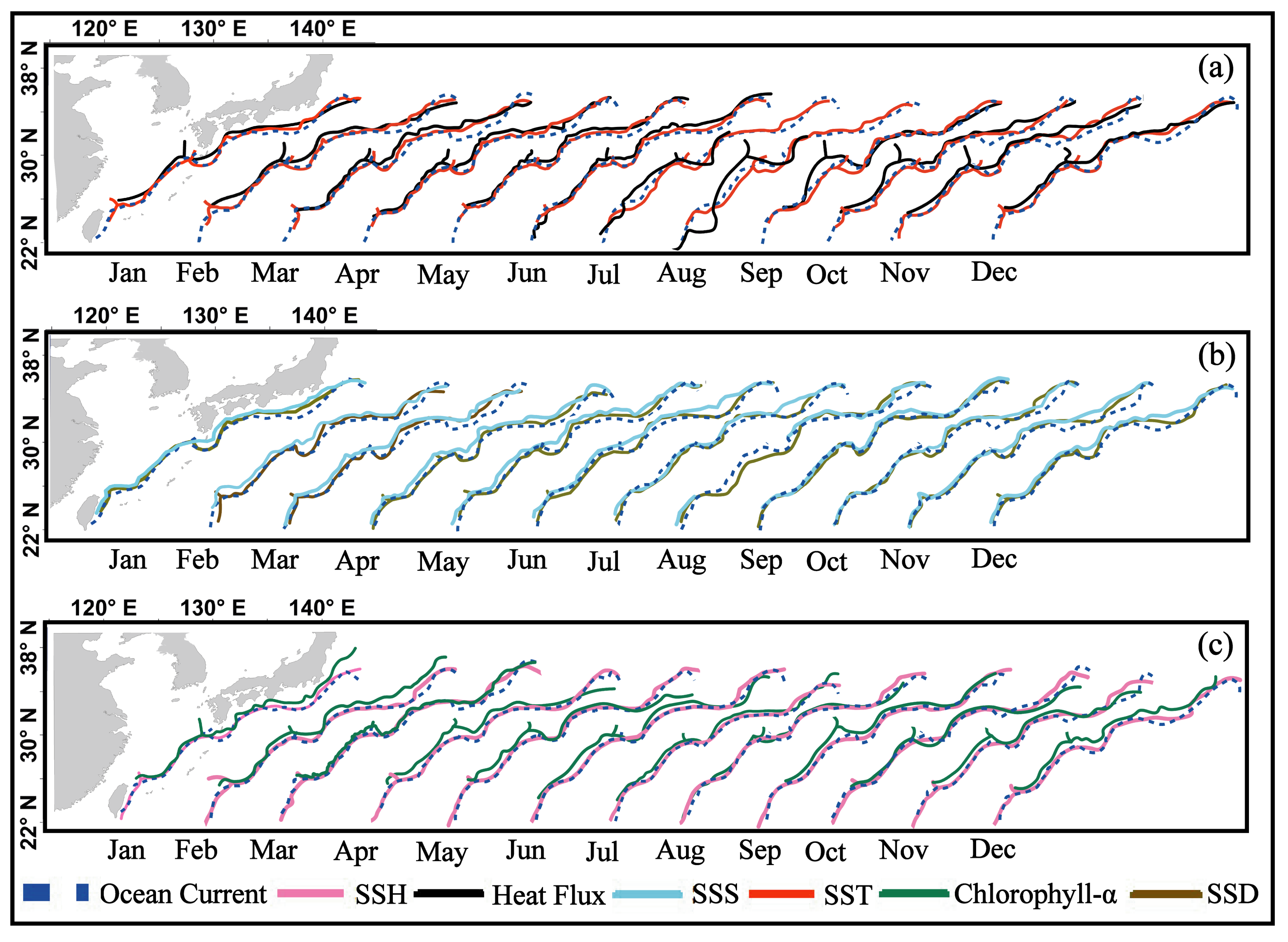
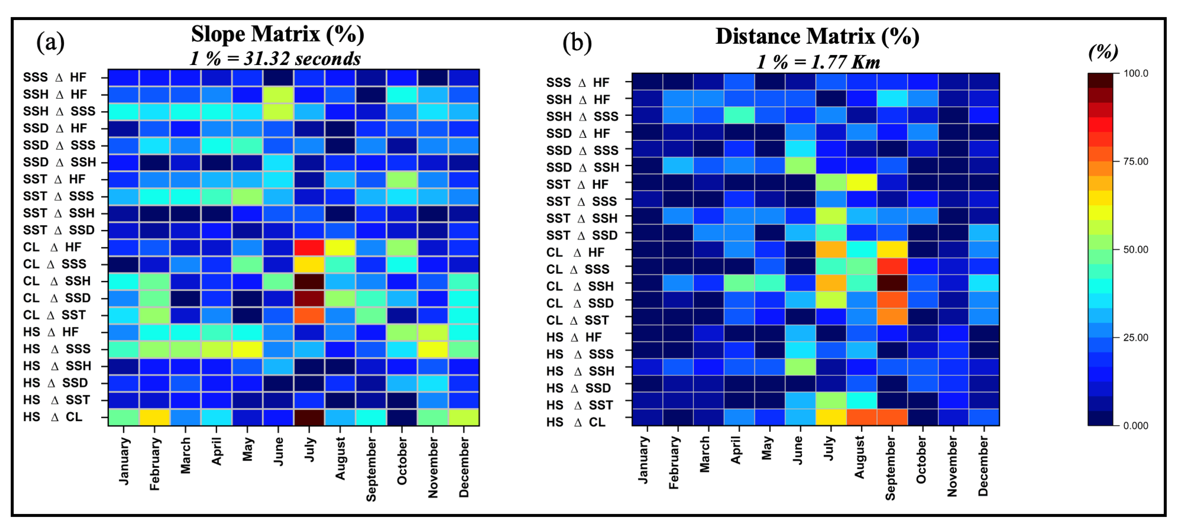
2.3.6. Correlation and Proximity Analysis
3. Results
3.1. Mapping Kuroshio Ocean Front by Utilizing Methodology from Previous Related Studies
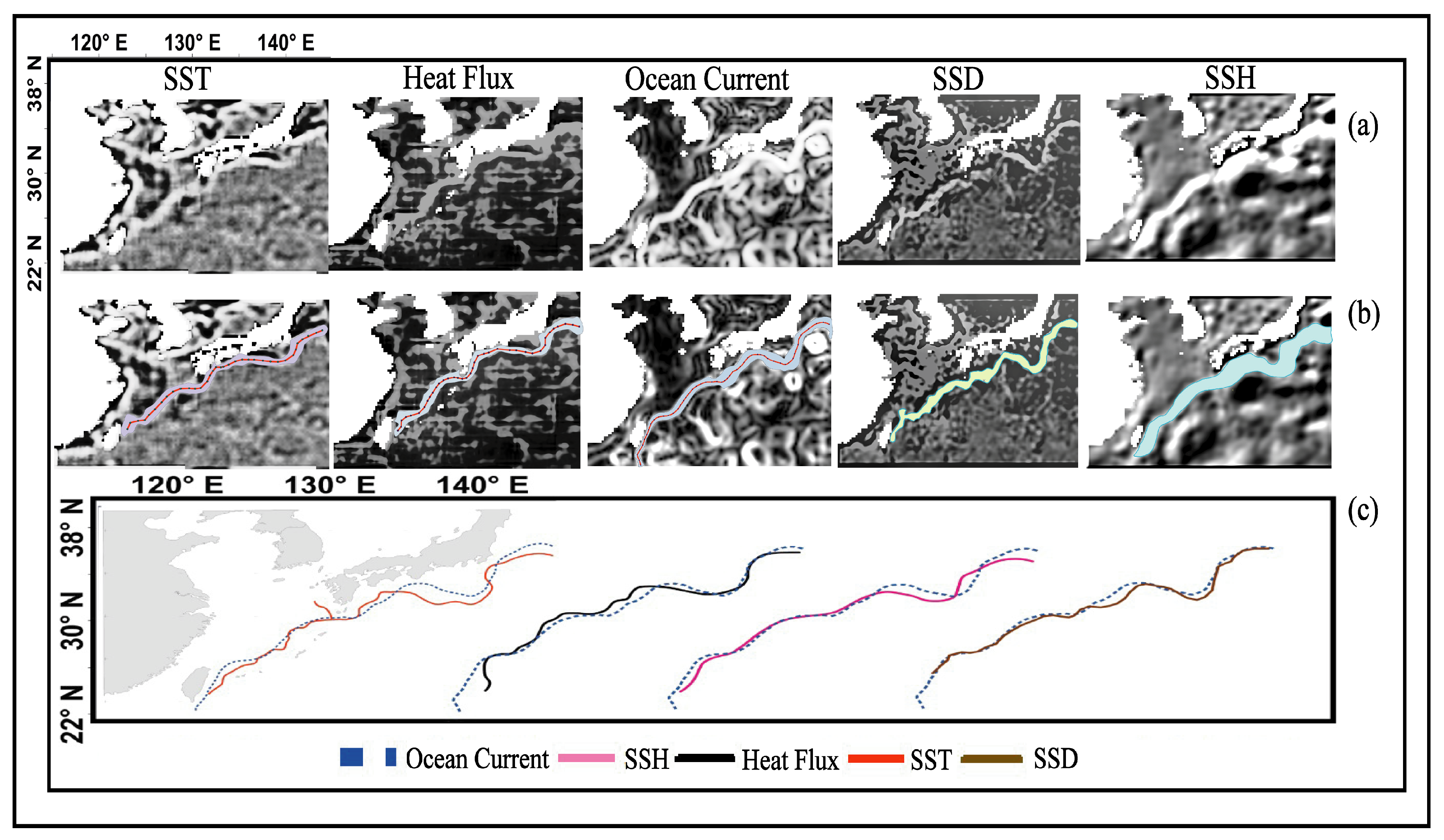
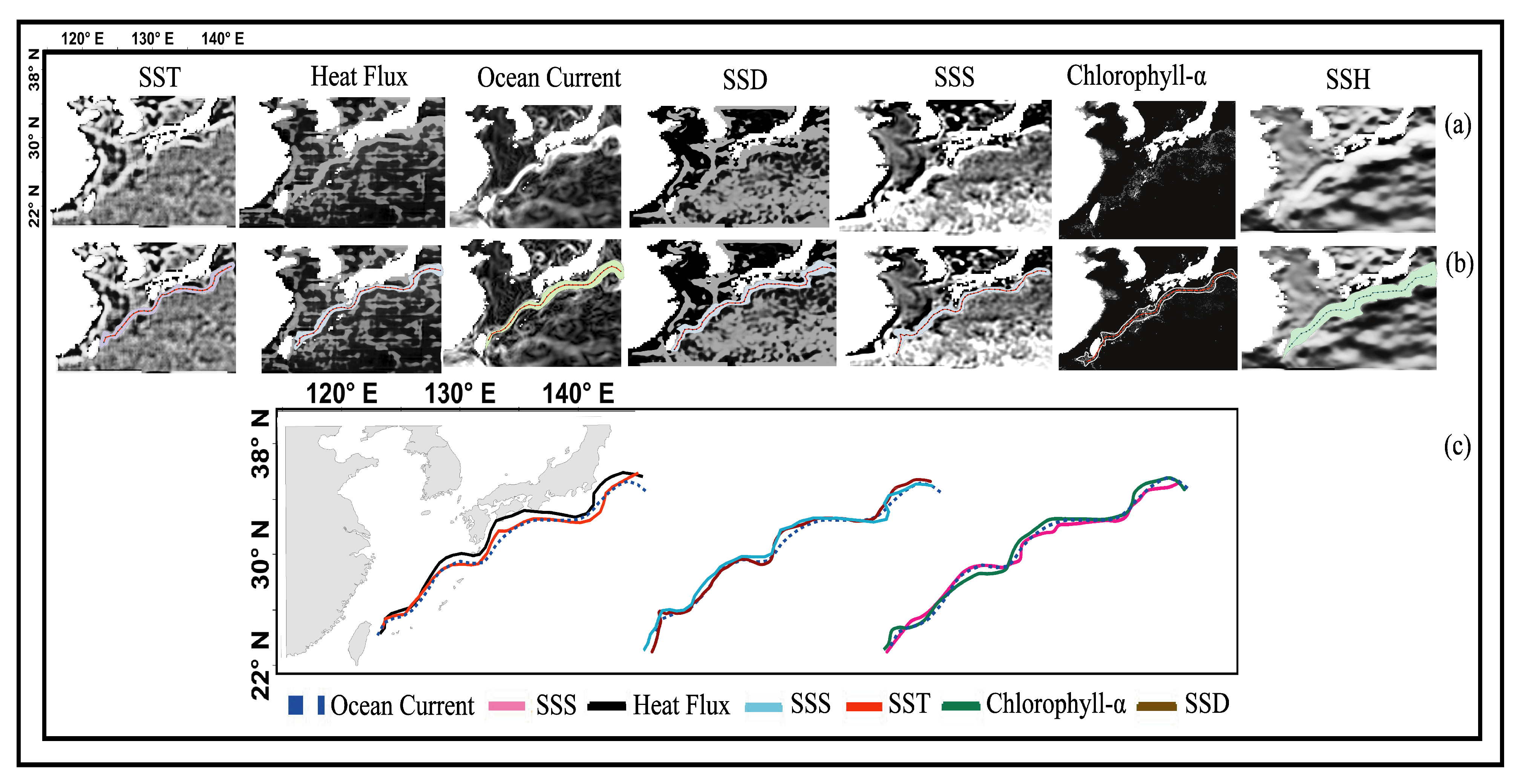
3.2. Detection of Kuroshio from Satellite Data
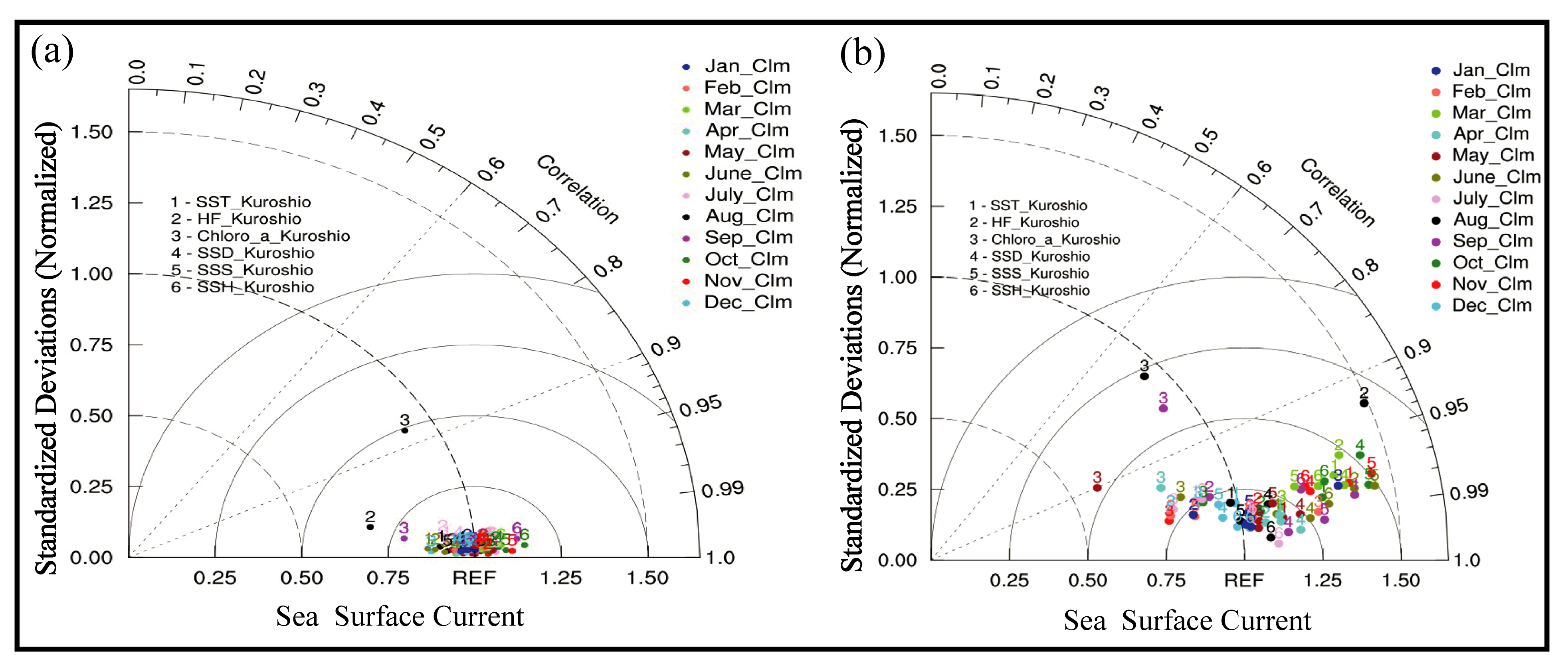
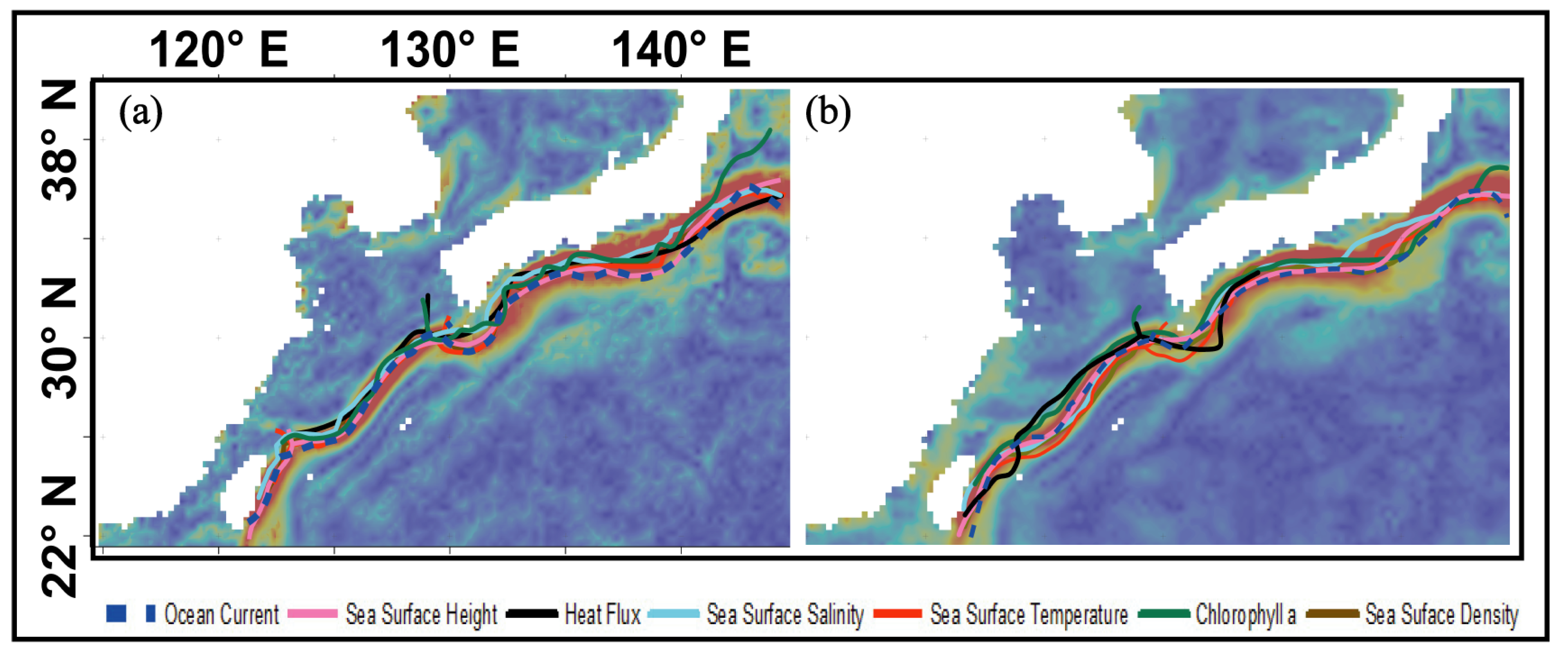
3.3. Inter-Comparison of Kuroshio Centerline from Climatology
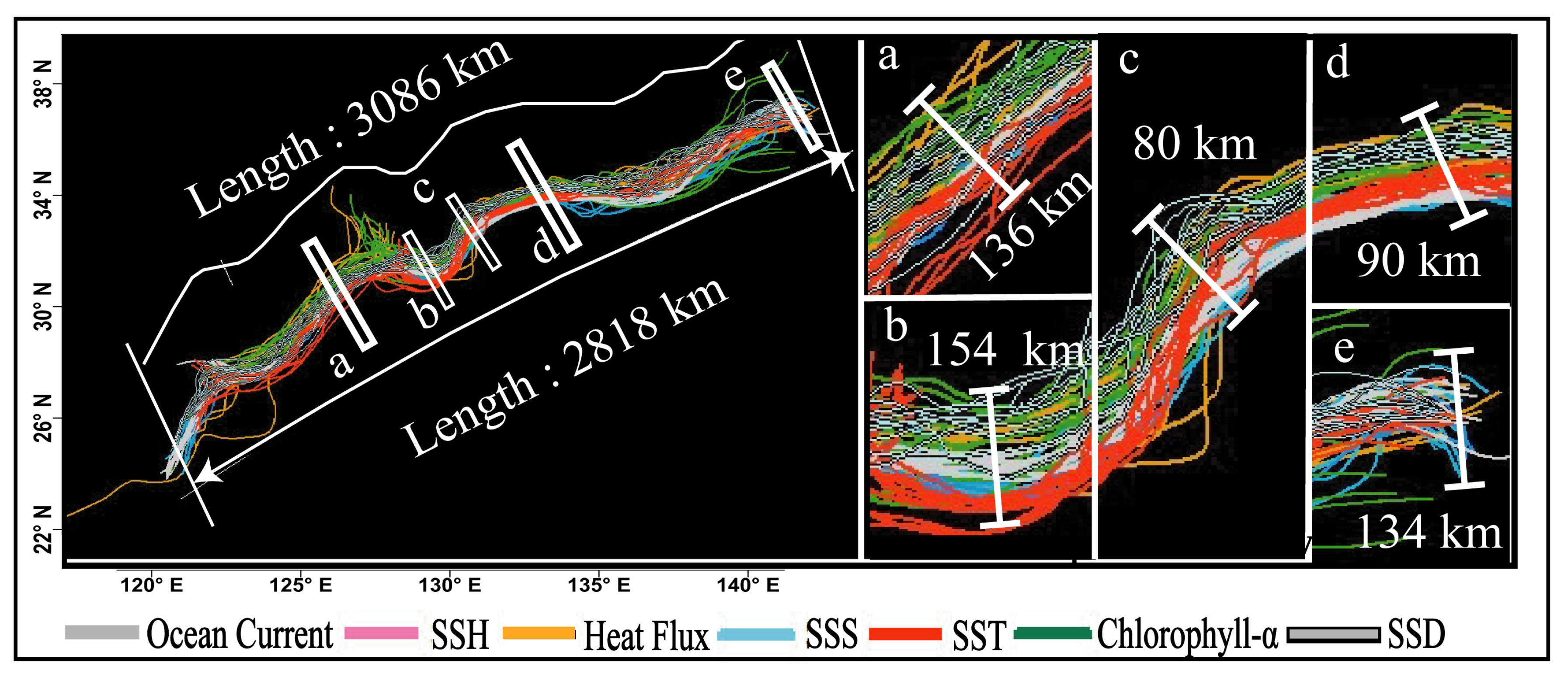
3.4. Kuroshio from Weekly and Seasonal Data
4. Discussion
5. Conclusions
Author Contributions
Funding
Institutional Review Board Statement
Informed Consent Statement
Data Availability Statement
Acknowledgments
Conflicts of Interest
References
- Caiyun, Z.; Ge, C. SST variations of the Kuroshio from AVHRR observation. Chin. J. Oceanol. Limnol. 2006, 24, 345–351. [Google Scholar] [CrossRef]
- Nayak, R.; Mishra, S.; Satyesh Ghetiya, N.P.; Choudhury, S.; Seshasai, M. Remote Sensing Application in Satellite Oceanography. Remote Sens. 2018, 93, 156–165. [Google Scholar]
- Takano, I.; Imawaki, S.; Kunishi, H. TS dynamic height calculation in the Kuroshio region. La Mer 1981, 19, 75–84. [Google Scholar]
- Yamamoto, T.; Nishizawa, S.; Taniguchi, A. Formation and retention mechanisms of phytoplankton peak abundance in the Kuroshio front. J. Plankton Res. 1988, 10, 1113–1130. [Google Scholar] [CrossRef]
- Saito, H. The Kuroshio: Its recognition, scientific activities and emerging issues. In Kuroshio Current: Physical, Biogeochemical, and Ecosystem Dynamics; Geophysical Monograph Series 243; American Geophysical Union: Washington, DA, USA, 2019; pp. 1–11. [Google Scholar]
- Kawamura, H.; Mizuno, K.; Toba, Y. Formation process of a warm-core ring in the Kuroshio-Oyashio frontal zone—December 1981–October 1982. Deep. Sea Res. Part A Oceanogr. Res. Pap. 1986, 33, 1617–1640. [Google Scholar] [CrossRef]
- Toda, T. Movement of the surface front induced by Kuroshio frontal eddy. J. Geophys. Res. Ocean. 1993, 98, 16331–16339. [Google Scholar] [CrossRef]
- Yuan, D.; Han, W.; Hu, D. Surface Kuroshio path in the Luzon Strait area derived from satellite remote sensing data. J. Geophys. Res. Ocean. 2006, 111. [Google Scholar] [CrossRef] [Green Version]
- Ji, C.; Zhang, Y. Investigation of the Chlorophyll-A Concentration Response to Sea Surface Temperature (SST) in the East China Sea. In Proceedings of the IGARSS 2019–2019 IEEE International Geoscience and Remote Sensing Symposium, Yokohama, Japan, 28 July–2 August 2019; pp. 8003–8006. [Google Scholar]
- Hickox, R.; Belkin, I.; Cornillon, P.; Shan, Z. Climatology and seasonal variability of ocean fronts in the East China, Yellow and Bohai Seas from satellite SST data. Geophys. Res. Lett. 2000, 27, 2945–2948. [Google Scholar] [CrossRef] [Green Version]
- Ullman, D.S.; Cornillon, P.C. Satellite-derived sea surface temperature fronts on the continental shelf off the northeast US coast. J. Geophys. Res. Ocean. 1999, 104, 23459–23478. [Google Scholar] [CrossRef]
- Legeckis, R.; Brown, C.W.; Chang, P.S. Geostationary satellites reveal motions of ocean surface fronts. J. Mar. Syst. 2002, 37, 3–15. [Google Scholar] [CrossRef]
- Marumo, R. Diatom plankton in the south of Cape Shionomisaki in 1953. Oceanogr. Mag. 1954, 6, 145. [Google Scholar]
- Kawarada, Y. Diatoms in the Kuroshio waters neighboring Japan. Inform. Bull. Planktol. Jpn. 1965, 12, 8–16. [Google Scholar]
- Kuroda, K. Chlorophyll distribution in the Kuroshio region, south of Japan. Kousuiken Note. Sora Umi 1987, 9, 19–29. [Google Scholar]
- Imai, M. Seasonal variation of chlorophyll-a in the seas around Japan. Oceanogr. Mag. 1988, 38, 23–32. [Google Scholar]
- Hanzawa, M. Studies on the mechanism of formation of cold water in the Okhotsk Sea. In Report of Joint-Research on the Okhotsk Sea; Research Coordination Bureau, Science and Technology Agency Tokyo: Kawaguchi, Japan, 1981; pp. 66–131. [Google Scholar]
- Liu, Z.; Hou, Y. Kuroshio Front in the East China sea from satellite SST and remote sensing data. IEEE Geosci. Remote Sens. Lett. 2011, 9, 517–520. [Google Scholar] [CrossRef]
- Nagai, T.; Otsuka, K.; Nakano, H. The Research Advancements and Historical Episodes brought by the Kuroshio Flowing across Generations. In Kuroshio Current: Physical, Biogeochemical, and Ecosystem Dynamics; American Geophysical Union (AGU): Washington, DC, USA, 2019; pp. 13–22. [Google Scholar] [CrossRef]
- Garcia-Eidell, C.; Comiso, J.C.; Dinnat, E.; Brucker, L. Sea surface salinity distribution in the Southern Ocean as observed from space. J. Geophys. Res. Ocean. 2019, 124, 3186–3205. [Google Scholar] [CrossRef]
- Su, F.C.; Tseng, R.S.; Ho, C.R.; Lee, Y.H.; Zheng, Q. Detecting surface Kuroshio front in the Luzon strait from multichannel satellite data using neural networks. IEEE Geosci. Remote Sens. Lett. 2010, 7, 718–722. [Google Scholar] [CrossRef]
- Douglas, B.; McAdoo, D.; Cheney, R. Oceanographic and geophysical applications of satellite altimetry. Rev. Geophys. 1987, 25, 875–880. [Google Scholar] [CrossRef]
- Fu, L.L.; Cheney, R.E. Application of satellite altimetry to ocean circulation studies: 1987–1994. Rev. Geophys. 1995, 33, 213–223. [Google Scholar] [CrossRef]
- Fu, L.L.; Christensen, E.J.; Yamarone, C.A., Jr.; Lefebvre, M.; Menard, Y.; Dorrer, M.; Escudier, P. TOPEX/POSEIDON mission overview. J. Geophys. Res. Ocean. 1994, 99, 24369–24381. [Google Scholar] [CrossRef]
- Lagerloef, G.S.; Mitchum, G.T.; Lukas, R.B.; Niiler, P.P. Tropical Pacific near-surface currents estimated from altimeter, wind, and drifter data. J. Geophys. Res. Ocean. 1999, 104, 23313–23326. [Google Scholar] [CrossRef]
- Imawaki, S.; Uchida, H.; Ichikawa, H.; Fukasawa, M.; Umatani, S.i.; Group, A. Satellite altimeter monitoring the Kuroshio transport south of Japan. Geophys. Res. Lett. 2001, 28, 17–20. [Google Scholar] [CrossRef]
- Ma, C.; Wu, D.; Lin, X. Variability of surface velocity in the Kuroshio Current and adjacent waters derived from Argos drifter buoys and satellite altimeter data. Chin. J. Oceanol. Limnol. 2009, 27, 208–217. [Google Scholar] [CrossRef]
- Liu, Z.; Wu, L. Atmospheric Response to North Pacific SST: The Role ofOcean–Atmosphere Coupling. J. Clim. 2004, 17, 1859–1882. [Google Scholar] [CrossRef] [Green Version]
- Konda, M.; Imasato, N.; Shibata, A. A new method to determine near-sea surface air temperature by using satellite data. J. Geophys. Res. Ocean. 1996, 101, 14349–14360. [Google Scholar] [CrossRef]
- Murakami, H.; Kawamura, H. Relations between sea surface temperature and air-sea heat flux at periods from 1 day to 1 year observed at ocean buoy stations around Japan. J. Oceanogr. 2001, 57, 565–580. [Google Scholar] [CrossRef]
- Kubota, M.; Kano, A.; Muramatsu, H.; Tomita, H. Intercomparison of various surface latent heat flux fields. J. Clim. 2003, 16, 670–678. [Google Scholar] [CrossRef]
- Qiu, B.; Chen, S.; Hacker, P. Synoptic-scale air–sea flux forcing in the western North Pacific: Observations and their impact on SST and the mixed layer. J. Phys. Oceanogr. 2004, 34, 2148–2159. [Google Scholar] [CrossRef]
- Frankignoul, C.; Sennéchael, N. Observed influence of North Pacific SST anomalies on the atmospheric circulation. J. Clim. 2007, 20, 592–606. [Google Scholar] [CrossRef]
- Bond, N.A.; Cronin, M.F. Regional weather patterns during anomalous air–sea fluxes at the Kuroshio Extension Observatory (KEO). J. Clim. 2008, 21, 1680–1697. [Google Scholar] [CrossRef] [Green Version]
- Konda, M.; Ichikawa, H.; Tomita, H.; Cronin, M.F. Surface heat flux variations across the Kuroshio Extension as observed by surface flux buoys. J. Clim. 2010, 23, 5206–5221. [Google Scholar] [CrossRef] [Green Version]
- Cancet, M.; Griffin, D.; Cahill, M.; Chapron, B.; Johannessen, J.; Donlon, C. Evaluation of GlobCurrent surface ocean current products: A case study in Australia. Remote Sens. Environ. 2019, 220, 71–93. [Google Scholar] [CrossRef] [Green Version]
- Rio, M.H.; Mulet, S.; Picot, N. Beyond GOCE for the ocean circulation estimate: Synergetic use of altimetry, gravimetry, and in situ data provides new insight into geostrophic and Ekman currents. Geophys. Res. Lett. 2014, 41, 8918–8925. [Google Scholar] [CrossRef]
- Ablain, M.; Cazenave, A.; Larnicol, G.; Balmaseda, M.; Cipollini, P.; Faugère, Y.; Fernandes, M.; Henry, O.; Johannessen, J.; Knudsen, P.; et al. Improved sea level record over the satellite altimetry era (1993–2010) from the Climate Change Initiative project. Ocean. Sci. 2015, 11, 67–82. [Google Scholar] [CrossRef] [Green Version]
- Nkwinkwa Njouodo, A.S.; Koseki, S.; Keenlyside, N.; Rouault, M. Atmospheric signature of the Agulhas Current. Geophys. Res. Lett. 2018, 45, 5185–5193. [Google Scholar] [CrossRef]
- Sun, X. Analysis of the surface path of the Kuroshio in the East China Sea. In Essays on Investigation of Kuroshio; Ocean Press: Beijing, China, 1987; pp. 1–14. [Google Scholar]
- Kawabe, M. Spectral properties of sea level and time scales of Kuroshio path variations. J. Oceanogr. Soc. Jpn. 1987, 43, 111–123. [Google Scholar] [CrossRef]
- Kawabe, M. Variations of current path, velocity, and volume transport of the Kuroshio in relation with the large meander. J. Phys. Oceanogr. 1995, 25, 3103–3117. [Google Scholar] [CrossRef] [Green Version]
- Akitomo, K.; Masuda, S.; Awaji, T. Kuroshio path variation south of Japan: Stability of the paths in a multiple equilibrium regime. Oceanogr. Lit. Rev. 1997, 44, 1226–1227. [Google Scholar]
- Yamashiro, T.; Kawabe, M. Variations of the Kuroshio axis south of Kyushu in relation to the large meander of the Kuroshio. J. Oceanogr. 2002, 58, 487–503. [Google Scholar] [CrossRef]
- Maximenko, N. Index and composites of the Kuroshio meander south of Japan. J. Oceanogr. 2002, 58, 639–649. [Google Scholar] [CrossRef]
- Ebuchi, N.; Hanawa, K. Influence of mesoscale eddies on variations of the Kuroshio path south of Japan. J. Oceanogr. 2003, 59, 25–36. [Google Scholar] [CrossRef]
- Nagano, A.; Kawabe, M. Monitoring of generation and propagation of the Kuroshio small meander using sea level data along the southern coast of Japan. J. Oceanogr. 2004, 60, 879–892. [Google Scholar] [CrossRef]
- Usui, N.; Tsujino, H.; Fujii, Y.; Kamachi, M. Short-range prediction experiments of the Kuroshio path variabilities south of Japan. Ocean. Dyn. 2006, 56, 607–623. [Google Scholar] [CrossRef]
- Takahashi, W.; Kawamura, H. Detection method of the Kuroshio front using the satellite-derived chlorophyll—A images. Remote Sens. Environ. 2005, 97, 83–91. [Google Scholar] [CrossRef]
- Savchenko, V.K.; Bychkov, A.S.; Ilyichev, V.I. Kuroshio meandering and eddy formation to the East of Taiwan and their reflection in Potassium fields. Terr. Atmos. Ocean. Sci. 1995, 6, 1–11. [Google Scholar] [CrossRef]
- Nishimura, T.; Kobayashi, T.; Tanaka, S.; Sugimura, T. Satellite monitoring of oceanic turbulence around Japan Islands. Adv. Space Res. 1995, 16, 137–140. [Google Scholar] [CrossRef]
- Tang, T.; Tai, J.; Yang, Y. The flow pattern north of Taiwan and the migration of the Kuroshio. Cont. Shelf Res. 2000, 20, 349–371. [Google Scholar] [CrossRef]
- Liang, W.D.; Tang, T.; Yang, Y.; Ko, M.; Chuang, W.S. Upper-ocean currents around Taiwan. Deep. Sea Res. Part II Top. Stud. Oceanogr. 2003, 50, 1085–1105. [Google Scholar] [CrossRef]
- Tomita, H.; Kubota, M. Increase in turbulent heat flux during the 1990s over the Kuroshio/Oyashio extension region. Geophys. Res. Lett. 2005, 32. [Google Scholar] [CrossRef]
- Mariano, A.J.; Griffa, A.; Özgökmen, T.M.; Zambianchi, E. Lagrangian analysis and predictability of coastal and ocean dynamics 2000. J. Atmos. Ocean. Technol. 2002, 19, 1114–1126. [Google Scholar] [CrossRef] [Green Version]
- Beardsley, R.C.; Limeburner, R.; Owens, W.B. Drifter measurements of surface currents near Marguerite Bay on the western Antarctic Peninsula shelf during austral summer and fall, 2001 and 2002. Deep. Sea Res. Part II Top. Stud. Oceanogr. 2004, 51, 1947–1964. [Google Scholar] [CrossRef]
- Tseng, C.T.; Sun, C.L.; Yeh, S.Z.; Chen, S.C.; Liu, D.C.; Su, W.C. The Kuroshio variations from satellite-derived sea surface temperature and Argos satellite-tracking Lagrangian drifters. Int. J. Remote Sens. 2011, 32, 8725–8746. [Google Scholar] [CrossRef]
- Poulain, P.M.; Zambianchi, E. Surface circulation in the central Mediterranean Sea as deduced from Lagrangian drifters in the 1990s. Cont. Shelf Res. 2007, 27, 981–1001. [Google Scholar] [CrossRef]
- Hsin, Y.C.; Wu, C.R.; Shaw, P.T. Spatial and temporal variations of the Kuroshio east of Taiwan, 1982–2005: A numerical study. J. Geophys. Res. Ocean. 2008, 113. [Google Scholar] [CrossRef] [Green Version]
- Oka, E.; Kawabe, M. Dynamic structure of the Kuroshio south of Kyushu in relation to the Kuroshio path variations. J. Oceanogr. 2003, 59, 595–608. [Google Scholar] [CrossRef]
- Canny, J. A computational approach to edge detection. IEEE Trans. Pattern Anal. Mach. Intell. 1986, PAMI-8, 679–698. [Google Scholar] [CrossRef]
- Holyer, R.J.; Peckinpaugh, S.H. Edge detection applied to satellite imagery of the oceans. IEEE Trans. Geosci. Remote Sens. 1989, 27, 46–56. [Google Scholar] [CrossRef] [Green Version]
- Cayula, J.F.; Cornillon, P.; Holyer, R.; Peckinpaugh, S. Comparative study of two recent edge-detection algorithms designed to process sea-surface temperature fields. IEEE Trans. Geosci. Remote Sens. 1991, 29, 175–177. [Google Scholar] [CrossRef] [Green Version]
- Cayula, J.F.; Cornillon, P. Edge detection algorithm for SST images. J. Atmos. Ocean. Technol. 1992, 9, 67–80. [Google Scholar] [CrossRef]
- Cayula, J.F.; Cornillon, P. Multi-image edge detection for SST images. J. Atmos. Ocean. Technol. 1995, 12, 821–829. [Google Scholar] [CrossRef]
- Cayula, J.F.; Cornillon, P. Cloud detection from a sequence of SST images. Remote Sens. Environ. 1996, 55, 80–88. [Google Scholar] [CrossRef] [Green Version]
- Vázquez, D.P.; Atae-Allah, C.; Escamilla, P.L.L. Entropic approach to edge detection for SST images. J. Atmos. Ocean. Technol. 1999, 16, 970–979. [Google Scholar] [CrossRef]
- Ullman, D.S.; Cornillon, P.C. Evaluation of front detection methods for satellite-derived SST data using in situ observations. J. Atmos. Ocean. Technol. 2000, 17, 1667–1675. [Google Scholar] [CrossRef]
- Ullman, D.S.; Cornillon, P.C. Continental shelf surface thermal fronts in winter off the northeast US coast. Cont. Shelf Res. 2001, 21, 1139–1156. [Google Scholar] [CrossRef]
- Belkin, I.M.; Cornillon, P.; Ullman, D. Ocean fronts around Alaska from satellite SST data. In Proceedings of the American Meteorological Society’s 7th Conference on the Polar Meteorology and Oceanography and Joint Symposium on High-Latitude Climate Variations, Hyannis, MA, USA, 12–16 May 2003; Volume 12. [Google Scholar]
- Belkin, I.; Cornillon, P. Surface thermal fronts of the Okhotsk Sea. Pac. Oceanogr. 2004, 2, 6–19. [Google Scholar]
- Belkin, I.; Cornillon, P. Bering Sea thermal fronts from Pathfinder data: Seasonal and interannual variability. Pac. Oceanogr. 2005, 3, 6–20. [Google Scholar]
- Belkin, I.; Shan, Z.; Cornillon, P. Global survey of oceanic fronts from Pathfinder SST and in-situ data. In: Abstracts of the AGU 1998 Fall Meeting. Eos Trans. AGU 1998, 79 (Suppl. 45), F475. [Google Scholar]
- Belkin, I.; Cornillon, P.; Shan, Z. Global survey of ocean fronts from Pathfinder SST data. In Proceedings of the Oceanography Society Meeting, Miami Beach, FL, USA, 2–5 April 2001; p. 10. [Google Scholar]
- Belkin, I.M.; O’Reilly, J.E. An algorithm for oceanic front detection in chlorophyll and SST satellite imagery. J. Mar. Syst. 2009, 78, 319–326. [Google Scholar] [CrossRef]
- Kahru, M.; Håkansson, B.; Rud, O. Distributions of the sea-surface temperature fronts in the Baltic Sea as derived from satellite imagery. Cont. Shelf Res. 1995, 15, 663–679. [Google Scholar] [CrossRef]
- Mavor, T.P.; Bisagni, J.J. Seasonal variability of sea-surface temperature fronts on Georges Bank. Deep Sea Res. Part II Top. Stud. Oceanogr. 2001, 48, 215–243. [Google Scholar] [CrossRef]
- Nieto, K.; Demarcq, H. Multi-image edge detection on SST and chlorophyll satellite images in northern Chile. In Report of the Workshop on Indices of Mesoscale Structures (WKIMS); 2006; pp. 22–24. [Google Scholar]
- Breaker, L.C.; Mavor, T.P.; Broenkow, W.W. Mapping and Monitoring Large-Scale Ocean Fronts off the California Coast Using Imagery from the GOES-10 Geostationary Satellite; The Regents of the University of California: Oakland, CA, USA, 2005. [Google Scholar]
- Kostianoy, A.G.; Ginzburg, A.I.; Frankignoulle, M.; Delille, B. Fronts in the Southern Indian Ocean as inferred from satellite sea surface temperature data. J. Mar. Syst. 2004, 45, 55–73. [Google Scholar] [CrossRef] [Green Version]
- Moore, J.K.; Abbott, M.R.; Richman, J.G. Variability in the location of the Antarctic Polar Front (90–20 W) from satellite sea surface temperature data. J. Geophys. Res. Ocean. 1997, 102, 27825–27833. [Google Scholar] [CrossRef] [Green Version]
- Moore, J.K.; Abbott, M.R.; Richman, J.G. Location and dynamics of the Antarctic Polar Front from satellite sea surface temperature data. J. Geophys. Res. Ocean. 1999, 104, 3059–3073. [Google Scholar] [CrossRef]
- Kazmin, A.S.; Rienecker, M.M. Variability and frontogenesis in the large-scale oceanic frontal zones. J. Geophys. Res. Ocean. 1996, 101, 907–921. [Google Scholar] [CrossRef]
- Shimada, T.; Sakaida, F.; Kawamura, H.; Okumura, T. Application of an edge detection method to satellite images for distinguishing sea surface temperature fronts near the Japanese coast. Remote Sens. Environ. 2005, 98, 21–34. [Google Scholar] [CrossRef]
- Castelao, R.M.; Mavor, T.P.; Barth, J.A.; Breaker, L.C. Sea surface temperature fronts in the California Current System from geostationary satellite observations. J. Geophys. Res. Ocean. 2006, 111. [Google Scholar] [CrossRef] [Green Version]
- Civco, D.L. Artificial neural networks for land-cover classification and mapping. Int. J. Geogr. Inf. Sci. 1993, 7, 173–186. [Google Scholar] [CrossRef]
- Erol, H.; Akdeniz, F. A new supervised classification method for quantitative analysis of remotely-sensed multi-spectral data. Int. J. Remote Sens. 1998, 19, 775–782. [Google Scholar] [CrossRef]
- Flygare, A.M. A comparison of contextual classification methods using Landsat TM. Int. J. Remote Sens. 1997, 18, 3835–3842. [Google Scholar] [CrossRef]
- Jenks, G.F. The data model concept in statistical mapping. Int. Yearb. Cartogr. 1967, 7, 186–190. [Google Scholar]
- Goodchild, M.; Haining, R.; Wise, S. Integrating GIS and spatial data analysis: Problems and possibilities. Int. J. Geogr. Inf. Syst. 1992, 6, 407–423. [Google Scholar] [CrossRef]
- Osaragi, T. Classification Methods for Spatial Data Representation; Centre for Advanced Spatial Analysis (UCL): London, UK, 2002. [Google Scholar]
- Poulain, P.M. Adriatic Sea surface circulation as derived from drifter data between 1990 and 1999. J. Mar. Syst. 2001, 29, 3–32. [Google Scholar] [CrossRef]
- Barkley, R. The Kuroshio current. Sci. J. 1970, 6, 54–60. [Google Scholar]
- Macdonald, A.M.; Wunsch, C. An estimate of global ocean circulation and heat fluxes. Nature 1996, 382, 436–439. [Google Scholar] [CrossRef]
- Nitani, H. Beginning of the Kuroshio. In Kuroshio, Physical Aspect of the Japan Current; University of Washington Press: Seattle, WA, USA, 1972. [Google Scholar]
- Feng, M.; Mitsudera, H.; Yoshikawa, Y. Structure and variability of the Kuroshio Current in Tokara Strait. J. Phys. Oceanogr. 2000, 30, 2257–2276. [Google Scholar] [CrossRef] [Green Version]
- Nakamura, H.; Ichikawa, H.; Nishina, A.; Lie, H.J. Kuroshio path meander between the continental slope and the Tokara Strait in the East China Sea. J. Geophys. Res. Ocean. 2003, 108. [Google Scholar] [CrossRef]
- Nitani, H. On the phase velocity of the large meander of the Kuroshio off Kyushu and Enshu-Nada: Large meander of the Kuroshio in 1975–1980 (III). Rep. Hydrogr. Res. 1982, 17, 229–239. [Google Scholar]
- Andres, M.; Jan, S.; Sanford, T.B.; Mensah, V.; Centurioni, L.R.; Book, J.W. Mean structure and variability of the Kuroshio from northeastern Taiwan to southwestern Japan. Oceanography 2015, 28, 84–95. [Google Scholar] [CrossRef] [Green Version]
- Rio, M.; Mulet, S.; Picot, N. New global Mean Dynamic Topography from a GOCE geoid model, altimeter measurements and oceanographic in-situ data. In Proceedings of the ESA living Planet Symposium, Edinburgh, UK, 9–13 September 2013. [Google Scholar]
- Ubelmann, C.; Klein, P.; Fu, L.L. Dynamic interpolation of sea surface height and potential applications for future high-resolution altimetry mapping. J. Atmos. Ocean. Technol. 2015, 32, 177–184. [Google Scholar] [CrossRef] [Green Version]
- Reynolds, R.W.; Rayner, N.A.; Smith, T.M.; Stokes, D.C.; Wang, W. An improved in situ and satellite SST analysis for climate. J. Clim. 2002, 15, 1609–1625. [Google Scholar] [CrossRef]
- Reynolds, R.W.; Smith, T.M.; Liu, C.; Chelton, D.B.; Casey, K.S.; Schlax, M.G. Daily high-resolution-blended analyses for sea surface temperature. J. Clim. 2007, 20, 5473–5496. [Google Scholar] [CrossRef]
- Huang, B.; Banzon, V.F.; Freeman, E.; Lawrimore, J.; Liu, W.; Peterson, T.C.; Smith, T.M.; Thorne, P.W.; Woodruff, S.D.; Zhang, H.M. Extended reconstructed sea surface temperature version 4 (ERSST. v4). Part I: Upgrades and intercomparisons. J. Clim. 2015, 28, 911–930. [Google Scholar] [CrossRef] [Green Version]
- Huang, B.; L’Heureux, M.; Hu, Z.Z.; Zhang, H.M. Ranking the strongest ENSO events while incorporating SST uncertainty. Geophys. Res. Lett. 2016, 43, 9165–9172. [Google Scholar] [CrossRef]
- Yu, L.; Weller, R.A. Objectively analyzed air–sea heat fluxes for the global ice-free oceans (1981–2005). Bull. Am. Meteorol. Soc. 2007, 88, 527–540. [Google Scholar] [CrossRef] [Green Version]
- Yu, C.; Hu, D.; Wang, S.; Chen, S.; Wang, Y. Estimation of anthropogenic heat flux and its coupling analysis with urban building characteristics—A case study of typical cities in the Yangtze River Delta, China. Sci. Total Environ. 2021, 774, 145805. [Google Scholar] [CrossRef]
- Song, X.; Yu, L. High-latitude contribution to global variability of air–sea sensible heat flux. J. Clim. 2012, 25, 3515–3531. [Google Scholar] [CrossRef] [Green Version]
- Rousseaux, C.S.; Gregg, W.W. Recent decadal trends in global phytoplankton composition. Glob. Biogeochem. Cycles 2015, 29, 1674–1688. [Google Scholar] [CrossRef] [Green Version]
- Ford, D.; Barciela, R. Global marine biogeochemical reanalyses assimilating two different sets of merged ocean colour products. Remote Sens. Environ. 2017, 203, 40–54. [Google Scholar] [CrossRef]
- Platt, T.; Sathyendranath, S.; Forget, M.H.; White III, G.N.; Caverhill, C.; Bouman, H.; Devred, E.; Son, S. Operational estimation of primary production at large geographical scales. Remote Sens. Environ. 2008, 112, 3437–3448. [Google Scholar] [CrossRef]
- Ciavatta, S.; Kay, S.; Saux-Picart, S.; Butenschön, M.; Allen, J. Decadal reanalysis of biogeochemical indicators and fluxes in the North West European shelf-sea ecosystem. J. Geophys. Res. Ocean. 2016, 121, 1824–1845. [Google Scholar] [CrossRef] [Green Version]
- Sathyendranath, S.; Brewin, R.J.; Brockmann, C.; Brotas, V.; Calton, B.; Chuprin, A.; Cipollini, P.; Couto, A.B.; Dingle, J.; Doerffer, R.; et al. An ocean-colour time series for use in climate studies: The experience of the ocean-colour climate change initiative (OC-CCI). Sensors 2019, 19, 4285. [Google Scholar] [CrossRef] [Green Version]
- Pujol, M.I.; Faugère, Y.; Taburet, G.; Dupuy, S.; Pelloquin, C.; Ablain, M.; Picot, N. DUACS DT2014: The new multi-mission altimeter data set reprocessed over 20 years. Ocean. Sci. 2016, 12, 1067–1090. [Google Scholar] [CrossRef] [Green Version]
- SChmitt, R.W. Salinity and the global water cycle. Oceanography 2008, 21, 12–19. [Google Scholar] [CrossRef]
- Frankignoul, C.; Deshayes, J.; Curry, R. The role of salinity in the decadal variability of the North Atlantic meridional overturning circulation. Clim. Dyn. 2009, 33, 777–793. [Google Scholar] [CrossRef] [Green Version]
- Umbert, M.; Hoareau, N.; Turiel, A.; Ballabrera-Poy, J. New blending algorithm to synergize ocean variables: The case of SMOS sea surface salinity maps. Remote Sens. Environ. 2014, 146, 172–187. [Google Scholar] [CrossRef]
- Droghei, R.; Nardelli, B.B.; Santoleri, R. Combining in situ and satellite observations to retrieve salinity and density at the ocean surface. J. Atmos. Ocean. Technol. 2016, 33, 1211–1223. [Google Scholar] [CrossRef]
- Droghei, R.; Buongiorno Nardelli, B.; Santoleri, R. A new global sea surface salinity and density dataset from multivariate observations (1993–2016). Front. Mar. Sci. 2018, 5, 84. [Google Scholar] [CrossRef] [Green Version]
- Athick, A.M.A.; Naqvi, H.R. A method for compositing MODIS images to remove cloud cover over Himalayas for snow cover mapping. In Proceedings of the 2016 IEEE International Geoscience and Remote Sensing Symposium (IGARSS), Beijing, China, 10–15 July 2016; pp. 4901–4904. [Google Scholar]
- Mohammed, A.A.A.; Naqvi, H.R.; Firdouse, Z. An assessment and identification of avalanche hazard sites in Uri sector and its surroundings on Himalayan mountain. J. Mt. Sci. 2015, 12, 1499. [Google Scholar] [CrossRef]
- Belkin, I.; Mikhailichenko, Y.G. Thermohaline Structure of the Frontal Zone of the Northwest Pacific-Ocean at 160∘-E. Okeanologiya 1986, 26, 70–72. [Google Scholar]
- Paris, S.; Hasinoff, S.W.; Kautz, J. Local Laplacian filters: Edge-aware image processing with a Laplacian pyramid. ACM Trans. Graph. 2011, 30, 68. [Google Scholar] [CrossRef]
- Alcaras, E.; Parente, C.; Vallario, A. Automation of Pan-Sharpening Methods for Pléiades Images Using GIS Basic Functions. Remote Sens. 2021, 13, 1550. [Google Scholar] [CrossRef]
- Al-Amri, S.S.; Kalyankar, N.; Khamitkar, S. Image segmentation by using edge detection. Int. J. Comput. Sci. Eng. 2010, 2, 804–807. [Google Scholar]
- Senthilkumaran, N.; Rajesh, R. Image segmentation-a survey of soft computing approaches. In Proceedings of the 2009 International Conference on Advances in Recent Technologies in Communication and Computing, Kottayam, India, 27–28 October 2009; pp. 844–846. [Google Scholar]
- Al-Amri, S.S.; Kalyankar, N.; Khamitkar, S. Contrast stretching enhancement in remote sensing image. BIOINFO Sens. Netw. 2011, 1, 6–9. [Google Scholar]
- Mokhtar, N.; Harun, N.H.; Mashor, M.Y.; Mustafa, N.; Adollah, R.; Mohd Nasir, N.F. Image Enhancement Techniques Using Local, Global, Bright, Dark and Partial Contrast Stretching for Acute Leukemia Images; Perpustakaan Tuanku Syed Faizuddin Putra: Arau, Malaysia, 2009. [Google Scholar]
- Köhl, M.; Lister, A.; Scott, C.T.; Baldauf, T.; Plugge, D. Implications of sampling design and sample size for national carbon accounting systems. Carbon Balance Manag. 2011, 6, 1–20. [Google Scholar] [CrossRef] [PubMed] [Green Version]
- Wang, J.; Chen, A.; Yu, H. Sea Surface Temperature variations over Kuroshio in the East China Sea. E3S Web Conf. 2019, 131, 01048. [Google Scholar] [CrossRef]
- Lacorata, G.; Corrado, R.; Falcini, F.; Santoleri, R. FSLE analysis and validation of Lagrangian simulations based on satellite-derived GlobCurrent velocity data. Remote Sens. Environ. 2019, 221, 136–143. [Google Scholar] [CrossRef]
- He, Y.; Wang, X.; Li, D.; Xie, Z.; Chai, C. Typhoon disaster damage assessment and disaster situation web visu-alization based on NPP-VIIRS nighttime light remote sensing. In Proceedings of the AIIPCC 2021; The Second International Conference on Artificial Intelligence, Information Processing and Cloud Computing, Hangzhou, China, 26–28 June 2021; pp. 1–8. [Google Scholar]
- Kawai, H.; Saitoh, S.i. Secondary fronts, warm tongues and warm streamers of the Kuroshio Extension system. Deep. Sea Res. Part A Oceanogr. Res. Pap. 1986, 33, 1487–1507. [Google Scholar] [CrossRef]
- Guo, X.; Miyazawa, Y.; Yamagata, T. The Kuroshio onshore intrusion along the shelf break of the East China Sea: The origin of the Tsushima Warm Current. J. Phys. Oceanogr. 2006, 36, 2205–2231. [Google Scholar] [CrossRef]
- Xue, H.; Chai, F.; Pettigrew, N.; Xu, D.; Shi, M.; Xu, J. Kuroshio intrusion and the circulation in the South China Sea. J. Geophys. Res. Ocean. 2004, 109. [Google Scholar] [CrossRef] [Green Version]
- Donohue, K.A.; Watts, D.R.; Tracey, K.L.; Greene, A.D.; Kennelly, M. Mapping circulation in the Kuroshio Extension with an array of current and pressure recording inverted echo sounders. J. Atmos. Ocean. Technol. 2010, 27, 507–527. [Google Scholar] [CrossRef] [Green Version]
- Mizuno, K.; White, W.B. Annual and interannual variability in the Kuroshio current system. J. Phys. Oceanogr. 1983, 13, 1847–1867. [Google Scholar] [CrossRef]
- Belkin, I.; Cornillon, P. SST fronts of the Pacific coastal and marginal seas. Pac. Oceanogr. 2003, 1, 90–113. [Google Scholar]


| Candidates | Heat Flux | SST | Sea Surfac Current | Chlorophyll- | SSH | SSD | SSS |
|---|---|---|---|---|---|---|---|
| Natural Break Classification | ✓ | ✓ | ✓ | ||||
| Min-Max Stretch | ✓ | ✓ | ✓ | ||||
| Histogram Equalization | ✓ | ||||||
| Convolution Filter | ✓ | ✓ | ✓ | ||||
| Laplacian Filter | ✓ | ||||||
| Conditional Filter | ✓ | ||||||
| Standard Deviation Stretch_{n = 1} | ✓ | ✓ | ✓ | ||||
| Sharpening Filter | ✓ | ✓ | |||||
| North Gradient Filter | ✓ |
| Parameters | El-Nino(Seasonal) km | Maria(Weekly) km |
|---|---|---|
| HS Δ chlorophyll- | 47.5 | No Data |
| HS Δ SST | 29 | 9 |
| HS Δ SSD | 71 | 100 |
| HS Δ SSH | 50 | 0.3 |
| HS Δ SSS | 63 | No Data |
| HS Δ HF | 20.5 | 25 |
| chlorophyll- Δ SST | 76 | No Data |
| chlorophyll- Δ SSD | 23 | No Data |
| chlorophyll- Δ SSH | 2 | No Data |
| chlorophyll- Δ SSS | 15 | No Data |
| chlorophyll- Δ HF | 26 | No Data |
| SST Δ SSD | 100.1 | 91 |
| SST Δ SSH | 79 | 9 |
| SST Δ SSS | 91 | No Data |
| SST Δ HF | 50 | 18 |
| SSD Δ SSH | 20 | 100 |
| SSD Δ SSS | 8 | No Data |
| SSD Δ HF | 50 | 73 |
| SSH Δ SSS | 12 | No Data |
| SSH Δ HF | 29 | 27 |
| SSS Δ HF | 42 | No Data |
Publisher’s Note: MDPI stays neutral with regard to jurisdictional claims in published maps and institutional affiliations. |
© 2022 by the authors. Licensee MDPI, Basel, Switzerland. This article is an open access article distributed under the terms and conditions of the Creative Commons Attribution (CC BY) license (https://creativecommons.org/licenses/by/4.0/).
Share and Cite
AS, M.A.A.; Lee, S.-Y. A Combination of Spatial Domain Filters to Detect Surface Ocean Current from Multi-Sensor Remote Sensing Data. Remote Sens. 2022, 14, 332. https://doi.org/10.3390/rs14020332
AS MAA, Lee S-Y. A Combination of Spatial Domain Filters to Detect Surface Ocean Current from Multi-Sensor Remote Sensing Data. Remote Sensing. 2022; 14(2):332. https://doi.org/10.3390/rs14020332
Chicago/Turabian StyleAS, Mohammed Abdul Athick, and Shih-Yu Lee. 2022. "A Combination of Spatial Domain Filters to Detect Surface Ocean Current from Multi-Sensor Remote Sensing Data" Remote Sensing 14, no. 2: 332. https://doi.org/10.3390/rs14020332