An Efficient Algorithm for Ocean-Front Evolution Trend Recognition

Abstract

Marine hydrological elements are of vital importance in marine surveys. The evolution of these elements can have a profound effect on the relationship between human activities and marine hydrology. Therefore, the detection and explanation of the evolution laws of marine hydrological elements are urgently needed. In this paper, a novel method, named Evolution Trend Recognition (ETR), is proposed to recognize the trend of ocean fronts, being the most important information in the ocean dynamic process. Therefore, in this paper, we focus on the task of ocean-front trend classification. A novel classification algorithm is first proposed for recognizing the ocean-front trend, in terms of the ocean-front scale and strength. Then, the GoogLeNet Inception network is trained to classify the ocean-front trend, i.e., enhancing or attenuating. The ocean-front trend is classified using the deep neural network, as well as a physics-informed classification algorithm. The two classification results are combined to make the final decision on the trend classification. Furthermore, two novel databases were created for this research, and their generation method is described, to foster research in this direction. These two databases are called the Ocean-Front Tracking Dataset (OFTraD) and the Ocean-Front Trend Dataset (OFTreD). Moreover, experiment results show that our proposed method on OFTreD achieves a higher classification accuracy, which is 97.5%, than state-of-the-art networks. This demonstrates that the proposed ETR algorithm is highly promising for trend classification.

1. Introduction

The ocean dynamic process contains essential factors that characterize and reflect the ocean hydrological status and phenomena. Detection, localization, and classification of their formation and interaction processes are essential in various ocean-related fields, such as fisheries and global warming. Several ocean-related variables have been identified for the ocean dynamic process, such as ocean currents, ocean tides, inner waves, ocean fronts, mesoscale vortices [1], etc. The oceanfront is an important branch of the ocean dynamic process [2,3,4]. Specifically, ocean fronts are located at the boundary between water masses with different properties [5,6], such as density, temperature, salinity, etc. Changes in the strength and scale of ocean fronts are some of the most vital subjects being studied, because they play an important role in the coupling of winds and the ocean processes [7,8]. For example, water masses in the ocean-front system have a great effect on air-sea exchange [9,10,11], activate the biological activity of the region [12], and absorb atmospheric carbon dioxide [13,14].

For marine fishing and marine environmental protection, it is vitally important to characterize the trend of the ocean front [15,16,17,18,19]. In fact, identifying the trend of an oceanfront is a difficult task, because simply working on short snippets cannot provide sufficient information to recognize it. The key to achieving high trend-recognition accuracy is to extract features from the consecutive frames, i.e., a video clip. The video sequence should include the whole process of an ocean-front trend. Usually, the length of a sequence is no more than 200 frames. In our dataset, we choose videos containing 5 to 200 frames. To a certain extent, action recognition is similar to ocean-front trend recognition. Recognizing the actions in a video, e.g., walking, jumping, etc., requires observing the entire motion process. Similarly, we have to consider a certain number of consecutive frames for recognizing the trend of an oceanfront, which is in either an enhancement or attenuation state.

In our previous work [20,21,22,23,24,25], both traditional machine-learning methods and deep neural networks were introduced to detect, recognize and predict ocean fronts and eddies. However, to the best of our knowledge, there is little previous work trying to recognize ocean-front trends based on oceanfront video sequences, but there are plenty of works trying to recognize or classify actions based on surveillance video sequences. Action classification [26,27,28] is an active field of research attracting increasing attention, due to its numerous potential applications in surveillance, video analysis, etc. The long-standing research on this classification task can be roughly divided into two categories. The first category relies on statistical feature extraction, followed by classifiers [29,30], while the second category is based on convolutional neural networks (CNNs). Examples of methods based on statistical features include [31,32,33]. However, these methods have limited generalization ability compared with CNNs. CNNs, which replace handcrafted features with “learned-from-data” features, have been successfully used for image classification [34,35]. Specifically, deep-learning-based methods [36,37,38,39,40] have achieved remarkable progress in video analysis.

According to our previous work, deep learning models are promising methods for ocean-front recognition and prediction. Thus, in this paper, we propose to use deep learning methods to classify ocean-front evolution trends. However, if deep learning models, such as CNNs, are directly applied to a video sequence, Karpathy et al. [41] found that the recognition performance achieved was inferior, compared with the state-of-the-art statistical features. Besides, inspired by the success of the region-proposal methods for object detection [42,43], some methods have attempted to extract temporal information from short snippets [28,44,45], by sparsely sampling from a long video sequence.

To improve the classification accuracy, a two-stream deep model [46], consisting of a spatial and a temporal CNN, was proposed, which achieved comparable performance with the most representative statistical features. One major limitation of the two-stream CNNs is that the method pays too much attention to the features extracted from a single RGB frame and the short-term motions, rather than the entire temporal information. Those frames, which are not within the selected short snippets of the video, may contain important temporal information, which can help improve the classification accuracy. Therefore, the deep model dismisses some useful temporal information. On the contrary, statistical features have an advantage in extracting the temporal information by using a specifically designed feature extraction algorithm based on prior knowledge. Therefore, in this paper, we propose a new fusion method for recognizing the ocean-front trend. We propose new statistical algorithms, which can extract temporal information from a video sequence, and we also apply a deep learning model to learn the deep feature from the video sequence, we then use weighted fusion to incorporate temporal information to improve classification accuracy. In our experiments, we prove that the proposed method can achieve high classification accuracy, better than using state-of-the-art deep-learning-based methods.

The novelty of this paper is twofold. (1) We introduce an Evolution Trend Recognition (ETR) method, which is based on classifiers with prior physical knowledge. The method not only gets rid of the complex operations required for selecting the frames with ocean fronts from a video sequence but can also aggregate the information extracted from different classification methods. (2) We have created a new database for ocean-front trend recognition, to encourage other researchers to evaluate their methods for ocean-front trend classification and facilitate them in using data-driven methods, especially deep-learning-based methods, to deal with this challenging task.

More specifically, our ETR method uses an effective mechanism to combine results from classification algorithms based on strength and scale, and employs deep-learning-based classification methods, based on the GoogLeNet Inception network [47], to recognize the ocean-front trend. Our experiment results show that the proposed ETR method achieves superior recognition performance over state-of-the-art methods on the Ocean-front Trend Dataset (OFTreD).

The remainder of this paper is organized as follows. The ETR framework and the process of building the OFTreD and Ocean-front Tracking Dataset (OFTraD), used in our experiments, are presented in detail in Section 2. Experimental results are presented in Section 3 and discussed in Section 4, and finally, Section 5 concludes this paper.

2. Materials and Methods

2.1. The Proposed Method

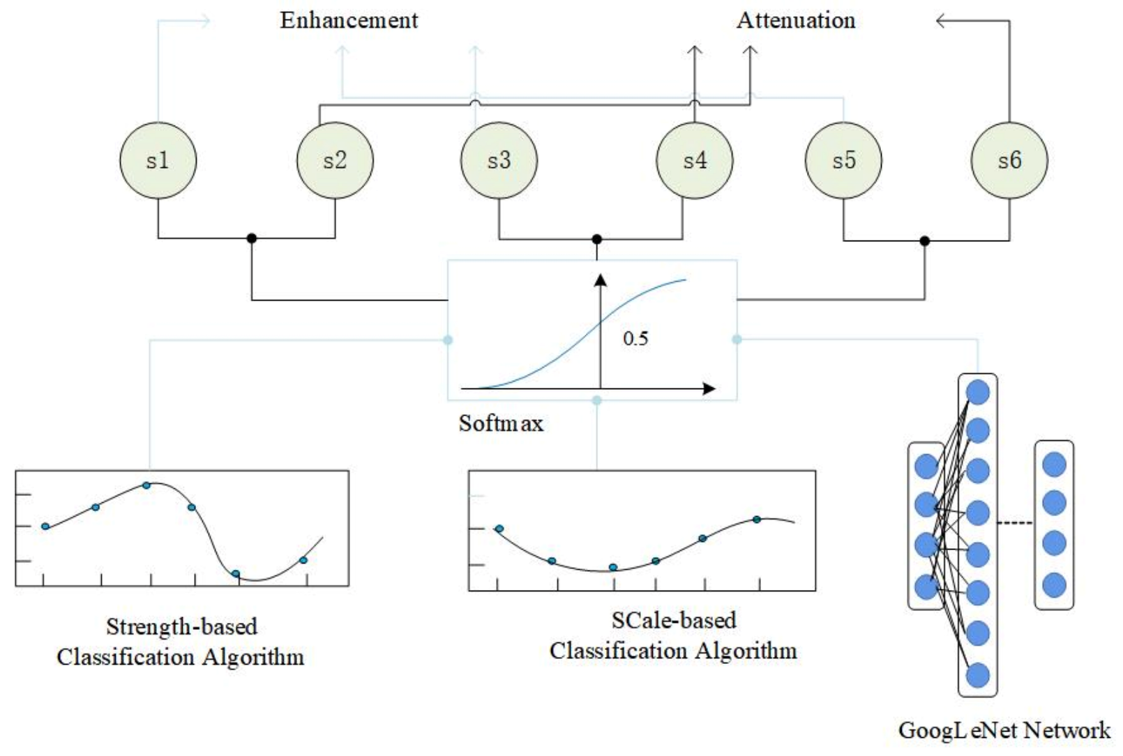
Extracting representative features from a video sequence is of prime importance for the task of ocean-front trend recognition. In this section, we will describe a novel idea for extracting discriminative features for recognizing the ocean-front trend, based on the analysis of a whole video. The key idea of the proposed method is shown in Figure 1, the proposed trend recognition method relies on the combination of the statistical algorithms and deep learning models. Softmax classifier is then applied for trend recognition of enhancement and attenuation. The proposed method avoids the complex operations required for selecting recommended frames, because the proposed method can extract representative temporal and deep features from the video sequence, and hence, it is efficient and effective.

In this section, we first described the network structure of the proposed recognition method in Section 2.1.1. Then, we described the ocean-front classification algorithm based on strength and scale feature in Section 2.1.2 and Section 2.1.3, respectively. In Section 2.1.4, we explained the feature matrices generation method. Then, we described the ocean-front trend classification algorithm based on the GoogLeNet Inception network in Section 2.1.5. Finally, we described the ocean-front tracking algorithm in Section 2.1.6.

2.1.1. Network Structure

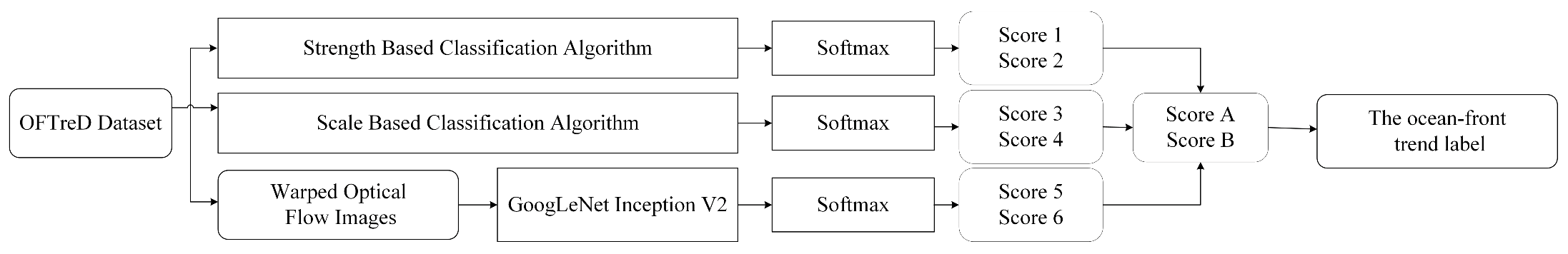
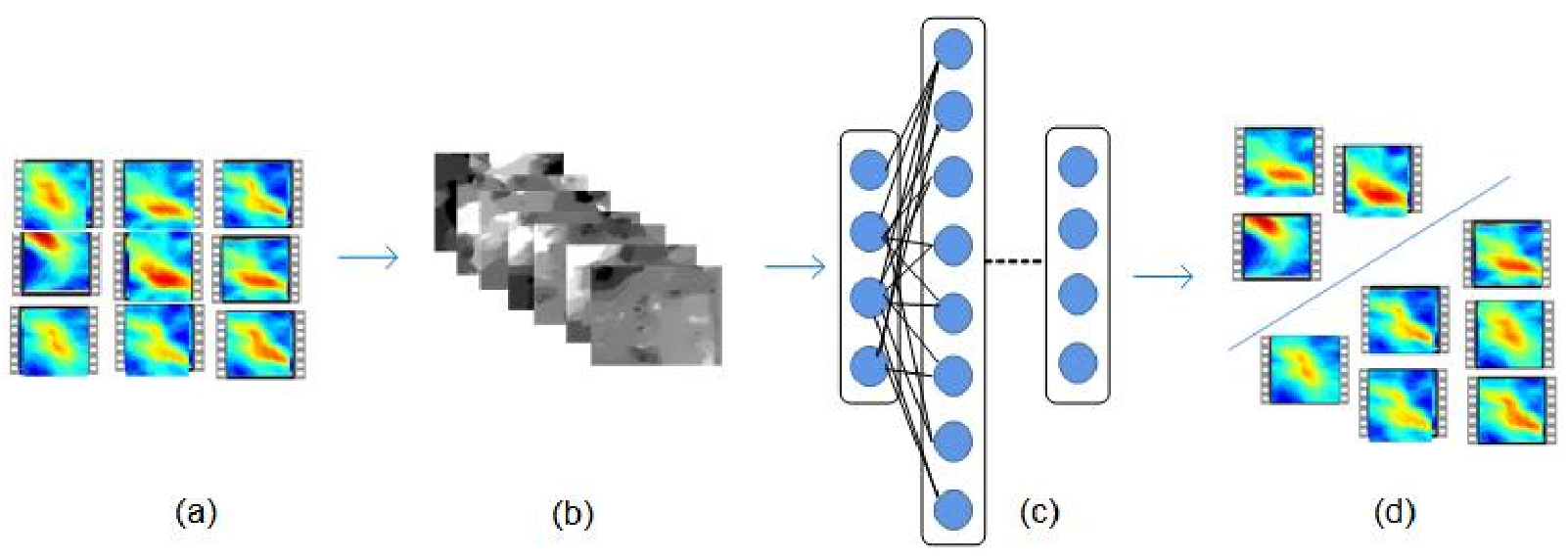
The proposed recognition framework, which is composed of three parallel networks, is depicted in Figure 2. The first and second networks are designed for trend classification, based on prior physical knowledge, which will be explained in Section 2.1.2 and Section 2.1.3. Their inputs are the video sequences from OFTreD. The OFTreD database is proposed for the ocean-front trend recognition task. The third network is also designed for ocean-front trend classification, based on GoogLeNet Inception, whose input is the optical flow images extracted from the video sequences in OFTreD. The first, second and third networks are integrated to classify the ocean-front trends. In this paper, two kinds of ocean-front trends are defined, namely, the enhancement trend and attenuation trend. In Figure 2, Score A and Score B are used to classify the ocean-front trend. The value of Score A denoted as $s_A$, represents the probability that an oceanfront enhancement trend, and that of Score B, denoted as $s_B$, represents the probability that an oceanfront has an attenuation trend. The scores $s_A$ and $s_B$ are computed as follows:

$$s_A=w_1\times s_1+w_2\times s_3+w_3\times s_5$$

(1)

$$s_B=w_1\times s_2+w_2\times s_4+w_3\times s_6$$

(2)

where $w_i,i=1,2,3$, are the weights, whose values will be discussed in Section 4. $s_j,$$j=1,...,6$, represents the value of Score j in Figure 2. The larger score of $s_A$ and $s_B$ will be used to determine the ocean-front trend category.

Each of the three proposed networks ends with a softmax layer, which outputs two scores to represent the probabilities of the input video sequence belonging to the enhancement or the attenuation trend. In total, six classification scores are generated. The six scores, i.e., Score 1 to Score 6, are used to classify whether the oceanfront is enhancing or attenuating. In our experiments, Scores 1, 3, and 5 are used to represent the probabilities of belonging to the enhancement trend, while the Scores 2, 4, and 6 are used to represent the attenuation trend. An ocean front in a video sequence belongs to either the “enhancement” class or the “attenuation” class. Finally, we integrate these six weighted scores to make the final decision on the trend class.

As shown in Figure 3, we also propose an oceanfront tracking algorithm to check whether the current input video sequence contains an oceanfront and where the ocean-front trend is in the video sequence. For this task, we train a GoogLeNet network on the OFTraD dataset.

The input of this network is the RGB images from OFTraD. The network is used to determine whether the input belongs to the background or the foreground. Those images that contain a tracking target, i.e., an oceanfront, belong to the foreground class, otherwise, they belong to the background class. Based on the location information carried by the input images, the output labeled images can be reconstructed into ocean-front video sequences, and then the ocean-front trend in the video sequences can be tracked.

2.1.2. Ocean-Front Classification Algorithm Based on Strength

The ocean-front trend classification algorithms based on strength and scale are trained on OFTreD. As shown in Figure 4, we calculate the mean intensity of the oceanfront to represent the oceanfront strength information of a frame. For the scale, we count the number of pixels of the oceanfront in each frame and use it to represent the scale information for the frame.

To improve the classification accuracy, we focus on the classification of ocean-front trends in a video sequence, rather than the snippets of a video. We analyze the overall ocean-front trend in a video sequence, based on the ocean-front strength and scale. The ocean-front strength can be represented by the numerical intensity of an oceanfront, while the ocean-front scale can be represented by the area of the existing oceanfront. Since the scale and strength of an oceanfront are highly correlated with the ocean-front trends, they can be used to effectively infer the trend of an oceanfront in a video sequence. Based on this prior knowledge, the scale and strength information of an ocean-front video sequence is used as an important reference for formulating the corresponding feature matrices $B_1$ and $B_2$$\in R^{(H-1)\times W}$, where W is the number of representative points extracted from a feature curve, and H represents the number of frames in the video. The details of computing the strength and scale feature matrices for an ocean-front video are shown in Algorithms 1 and 2, respectively. The method of generating a feature curve and extracting representative points from the feature curve will be described later in Section 2.1.4.

Algorithm 1 Classification Algorithm Based on Strength

1: Input: A video $v_i(x,y),i=1,...,H$, where H is the number of frames, and $(x,y)$ are the pixel coordinates 2: for$i=1$ to H do  Calculate the mean intensity of the ocean front in the frame i, denoted as $m_s\left(i\right)$, which is computed as follows: $$m_s\left(i\right)=\frac{1}{n_r\times n_c}\sum _{x=1}^{n_c}\sum _{y=1}^{n_r}{v}_i(x,y),$$ (3)  where $n_r$ and $n_c$ are the number of rows and columns, respectively, in a frame. 3: end for  Generate the mean intensity vector $a_1={[m_s\left(1\right)...m_s\left(H\right)]}^T$ for the video.  Apply a curve fitting technique to $a_1$ to form the feature curve $V_1$, and sample the curve $V_1$ with $(H-1)\times W$ points, where W is the number of representative points of each frame. In our experiments, W is set at 10. The sampled points then formulate a matrix $B_1\in R^{(H-1)\times W}$.  Then, use an average pooling filter to process the matrix $B_1$ to generate the resulting vector $c_1$. The resulting elements are denoted as $m_f$, and hence the vector $c_1={[m_f\left(1\right)...m_f\left(40\right)]}^T$, whose dimension is set at $40\times 1$ in our implementation. $c_1$ is the feature vector with unified dimension for trend classification.  Use the trained softmax to classify the vector $c_1$ 4: Output Classification scores $s_1,s_2$

Algorithm 2 Classification Algorithm Based on Scale

1: Input: A video containing H frames 2: for$i=1$ to H do  Count the number of ocean-front points in the frame i, denoted as $n_s\left(i\right)$, which are detected using the oceanfront detection method [22]. 3: end for  Count the number of ocean-front points for each of the H frames, to form the vector $a_2={[n_s\left(1\right)...n_s\left(H\right)]}^T$ for the video.  Apply a curve fitting technique to $a_2$ to form the curve $V_2$, and sample the curve $V_2$ with $(H-1)\times W$ points, where W is the number of representative points of each frame. In our experiments, W is set at 10. The sampled points then formulate a matrix $B_2\in R^{(H-1)\times W}$.  Then, use an average pooling filter to process the matrix $B_2$, get the resulting vector $c_2$. The resulting elements are denoted as $n_f$, and hence the vector $c_2={[n_f\left(1\right)...n_f\left(40\right)]}^T$, whose dimension is set at $40\times 1$ in our implementation. $c_2$ is the feature vector with unified dimension for trend classification.  Use the trained softmax to classify the vector $c_2$ 4: Output Classification scores $s_3,s_4$

2.1.3. Ocean-Front Classification Algorithm Based on Scale

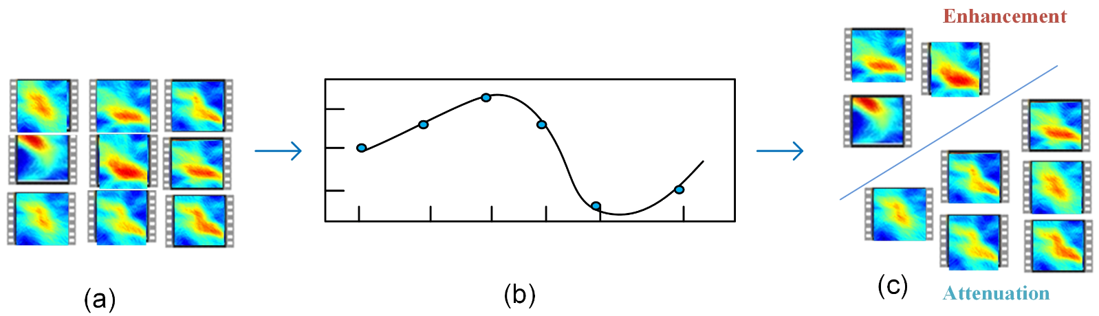
With the proposed algorithms, we will illustrate how to extract the strength and scale information about the oceanfront in a video sequence and the databases used for training and testing. Algorithm 1 is designed for recognizing ocean-front trends based on the strength of an oceanfront. To classify the trend, we need to compute the variations of the ocean-front strength. Since the strength of an oceanfront varies from point to point, we propose to use the mean intensity of an oceanfront in a frame to represent its strength. Similarly, Algorithm 2 is designed to classify the ocean-front trend based on its scale. The scale of an oceanfront is calculated based on the number of oceanfront points in a frame. The greater the number of ocean-front points, the larger the ocean-front scale is.

Here, the vectors $a_1$ and $a_2$ represent the strength and scale information, respectively, and the matrices $B_1$ and $B_2$ represent the points extracted from the corresponding curves, and the feature vectors $c_1$ and $c_2$ represent the filtered output from the corresponding matrices $B_1$ and $B_2$. Thus, the feature vectors $c_1$ and $c_2$ represent the processed strength and scale information, respectively. We use the feature vectors $c_1$ and $c_2$ to classify the ocean-front trend. Then, these feature vectors are sent to softmax for classification and generate the output $s_i,i=1,2,3,4$.

2.1.4. Feature Matrices Generation Method

In the ocean-front trend algorithms, the number of frames of different videos may be different, so the dimensions of the strength vector $a_1$ and the scale vector $a_2$ of different videos, as described in Algorithms 1 and 2, respectively, are different. To make the two vectors always have the same length, Algorithms 1 and 2 apply curve fitting to the vectors $a_1$ and $a_2$, then resamples the two curves with a fixed number of points. Specifically, as shown in Figure 5, we use the cubic polynomial interpolation method to fit the curves. With a fixed number of points on the curve, two matrices, $B_1$ and $B_2$$\in R^{(H-1)\times W}$, are generated. The matrices generation process is shown in Figure 6, starting from the point representing the strength/scale of the first frame, we sample points on the curve at regular intervals until the point that represents the last frame. We set $W=10$ in our experiments, because we need to extract more than 40 points from the curve. As analyzed in Section 4, the best vector dimension is $40\times 1$, too small will not meet the requirement, too large is unnecessary. After that, the matrices $B_1$ and $B_2$ are processed by three pooling filters to obtain fixed-dimensional vectors $c_1$ and $c_2$.

Given matrices $B_1$ and $B_2$$\in R^{(H-1)\times W}$, we vectorize the matrices $B_1$ and $B_2$ to acquire the feature vectors $b_1$ and $b_2$. The elements of the matrices $B_1$ and $B_2$ are denoted as $m_p$ and $n_p$, and hence the vector $b_1={[m_p\left(1\right)...m_p((H-1)\times W)]}^T$, $b_2={[n_p\left(1\right)...n_p((H-1)\times W)]}^T$, whose dimension is $\left[\right(H-1)\times W,1]$. As shown in Algorithm 3, according to the dimension of the matrices $B_1$ and $B_2$, we use different pooling filters. If the dimension of the feature vectors $b_1$ and $b_2$ is greater than $200\times 1$, average pooling is performed every 5 elements from the first and the last 50 elements in the feature vectors, that is $b_1[1:50,1]$, $b_1[(H-1)\times W-49:(H-1)\times W,1]$, $b_2[1:50,1]$, and $b_2[(H-1)\times W-49:(H-1)\times W,1]$, the filter size is $[5,1]$. Then, We assign $c_1[1:10,1]$, $c_1[31:40,1]$, $c_2[1:10,1]$, and $c_2[31:40,1]$ the value of the processed data. Then, the number of the remaining elements in the feature vectors $b_1$ and $b_2$ is $(H-1)\times W-100$. The pooling size is set at $\left(\right(H-1)\times W-100)/20\times 1$, the stride is set at $\left(\right(H-1)\times W-100)/20$. Average pooling is performed every $\left(\right(H-1)\times W-100)/20$ elements from $b_1[51:(H-1)\times W-50,1]$ and $b_2[51:(H-1)\times W-50,1]$. And then we assign $c_1[11:30,1]$ and $c_2[11:30,1]$ the value of the processed data.

Algorithm 3 The matrix processing method

1: Input: Matrices $B_1$ and $B_2$  Given matrices $B_1$ and $B_2$$\in R^{(H-1)\times W}$, we vectorize them to acquire its feature vectors $b_1$ and $b_2$. 2: if the dimension of the feature vectors $b_1$ and $b_2>[200,1]$ do  Average pooling is performed every 5 elements from the first 50 elements and the last 50 elements of the matrices, the filter size is $[5,1]$, the stride is 5. The processed data is assigned to $c_1$ and $c_2$. Average pooling is applied to the remaining elements in the feature vectors $b_1$ and $b_2$, the filter size is set according to the number of the remaining elements. 3: else if the dimension of the feature vectors $b_1$ and $b_2>[100,1]$ do  Average pooling is performed every 2 elements from the first and the last 30 elements, the filter size is $[2,1]$, the stride is 2. The processed data is assigned to $c_1$ and $c_2$. Average pooling is applied to the remaining elements in the feature vectors $b_1$ and $b_2$, the filter size is set according to the number of the remaining elements. 4: else do  The first and the last 15 elements of the vectorized matrices $B_1$ and $B_2$ are assigned to $c_1$ and $c_2$. Average pooling is applied to the remaining elements in the feature vectors $b_1$ and $b_2$, the filter size is set according to the number of the remaining elements. 5: Output Feature vectors $c_1$ and $c_2$

Otherwise, if the the dimension of the feature vectors $b_1$ and $b_2>[100,1]$, average pooling is performed every 2 elements from the first and the last 30 elements in the feature vectors, that is $b_1[1:30,1]$, $b_1[(H-1)\times W-29:(H-1)\times W,1]$, $b_2[1:30,1]$, and $b_2[(H-1)\times W-29:(H-1)\times W,1]$, the filter size is $[2,1]$. We assign $c_1[1:15,1]$, $c_1[26:40,1]$, $c_2[1:15,1]$, and $c_2[26:40,1]$ the value of the processed data. Then, the number of the remaining elements in the feature vectors $b_1$ and $b_2$ is $(H-1)\times W-60$. The pooling size is set at $\left(\right(H-1)\times W-60)/10\times 1$, the stride is set at $\left(\right(H-1)\times W-60)/10$. Average pooling is performed every $\left(\right(H-1)\times W-60)/10$ elements from $b_1[31:(H-1)\times W-30]$ and $b_2[31:(H-1)\times W-30]$. We assign $c_1[16:25,1]$ and $c_2[16:25,1]$ the value of the processed data, assign $c_1[11:30,1]$ and $c_2[11:30,1]$ the value of the processed data.

If the dimension of the feature vectors $b_1$ and $b_2<[100,1]$, we assign $c_1[1:15,1]$, $c_1[26:40,1]$, $c_2[1:15,1]$, and $c_2[26:40,1]$ the value of the first and the last 15 elements in the feature vectors, that is $b_1[1:15,1]$, $b_1[(H-1)\times W-14:(H-1)\times W,1]$, $b_2[1:15,1]$, and $b_2[(H-1)\times W-14:(H-1)\times W,1]$. Then, the number of the remaining elements in the feature vectors $b_1$ and $b_2$ is $(H-1)\times W-30$. The pooling size is set at $\left(\right(H-1)\times W-30)/10\times 1$, the stride is set at $\left(\right(H-1)\times W-30)/10$. Average pooling is performed every $\left(\right(H-1)\times W-30)/10$ elements of $b_1[16:(H-1)\times W-15,1]$ and $b_2[16:(H-1)\times W-15,1]$. Then we assign $c_1[16:25,1]$ and $c_2[16:25,1]$ the value of the processed data. In this way, feature vectors $c_1$ and $c_2$ can be constructed.

2.1.5. Ocean-Front Trend Classification Algorithm Based on GoogLeNet

The structure of the GoogLeNet is shown in Figure 7, the Inception block helps to handle the high-dimensional features and balance the width and depth of the network. It also enables the network to perform spatial aggregation in low-dimensional features without worrying about losing too much information. So, we apply this network to recognize the ocean-front trend and track the ocean-front location.

Figure 8 shows the process of the ocean-front trend recognition, GoogLeNet Inception network is employed to classify enhancement and attenuation of an oceanfront. The video input is warped by using the optical flow method. The GoogLeNet Inception network is trained and tested on the OFTreD dataset. The video sequence is first processed into warped optical flow images. Then, these images are sent to the GoogLeNet Inception network for classification. The softmax layer of the network generates the scores $s_i,i=5,6$, which are used to label the video sequence as an enhancement or attenuation trend.

2.1.6. Ocean-Front Tracking Algorithm Based on GoogLeNet

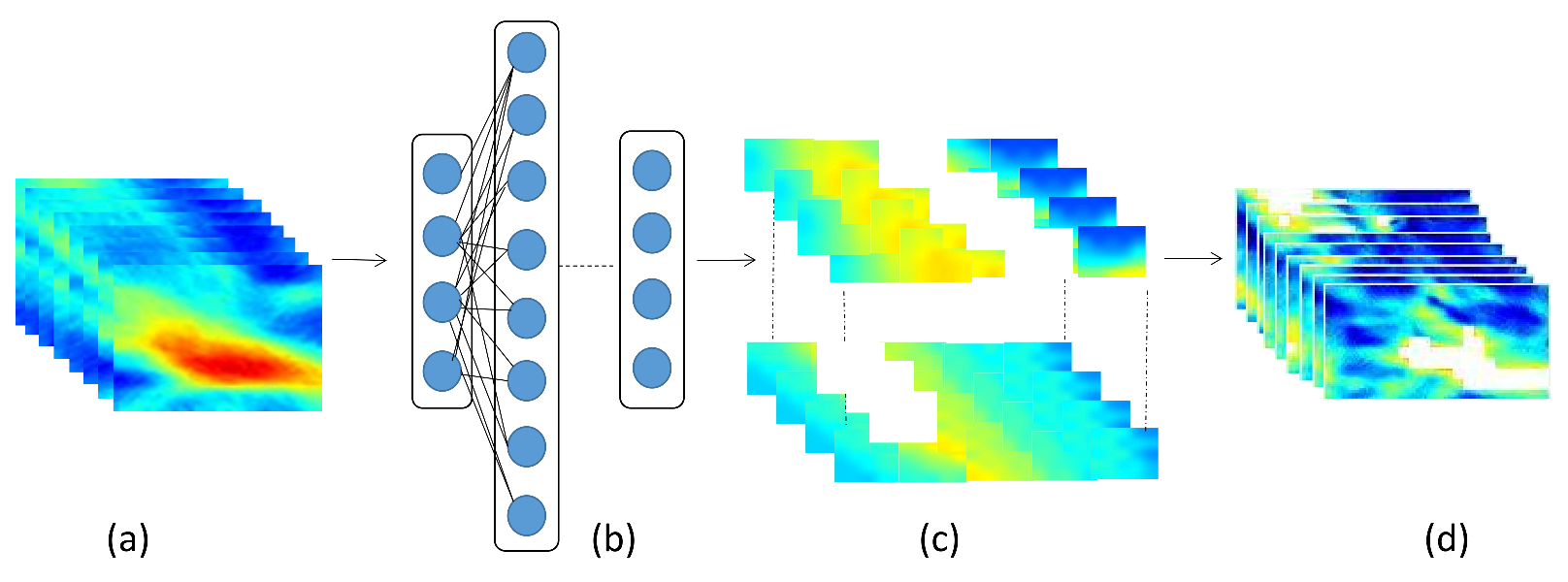
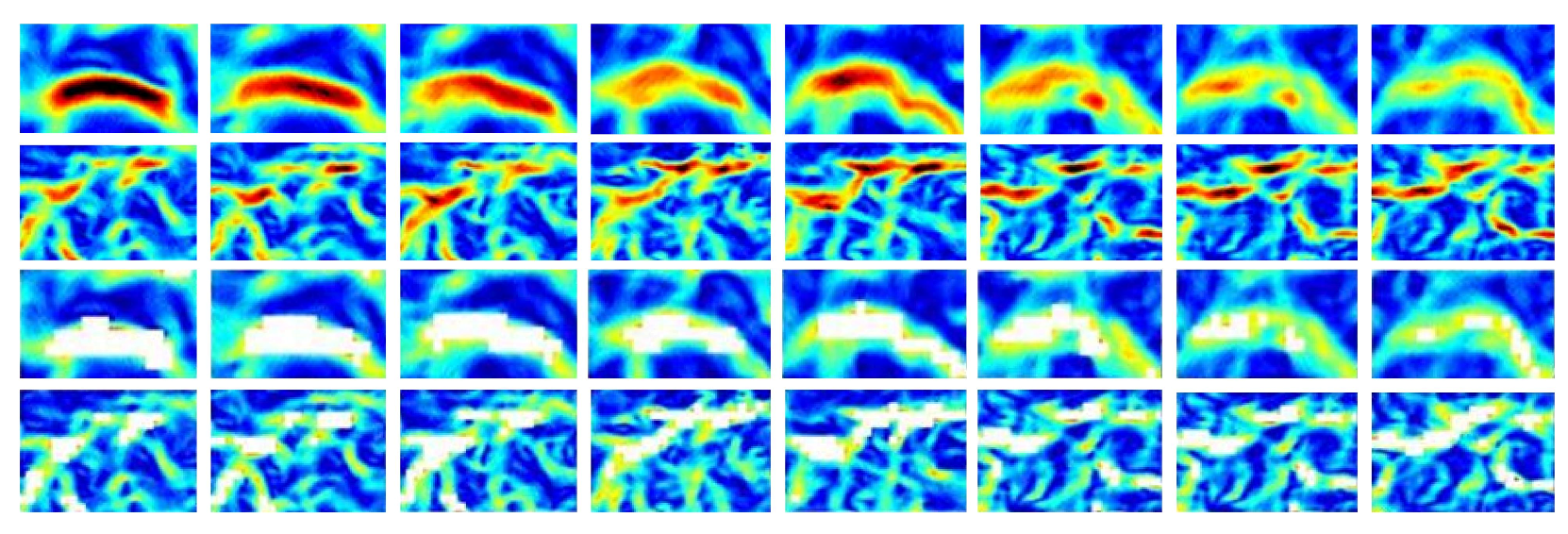
As shown in Figure 9, the ocean-front tracking algorithm is also based on the GoogLeNet Inception network. The network is used to classify image blocks into two classes: the oceanfront and the background. We first colored the oceanfront image blocks in white, and then, we further use the location information and place them back to the same position in the original frame. In this way, we can track the ocean-front location in a video sequence. It is worth noting that this network is trained on OFTraD, with 8000 and 2000 image blocks from the database used for training and testing, respectively.

The input of our algorithm is the image blocks and their time-position information. Firstly, we extract the RGB image blocks from each video sequence, and feed them into the GoogLeNet Inception network for classification. The color of the image blocks is set to white, if the image block is classified as the oceanfront. In our experiments, the block size is set to $5\times 5$, because this size can cover mesoscale ocean fronts. If the size of the blocks is too large, it will be hard to find the exact location of the background. If the block is too small, the classification accuracy will be reduced. Then, according to the corresponding time-position information, the blocks are put together to form a video sequence. When dividing an ocean-front frame into image blocks, we label their names with the time-position information, so that when getting their classification labels, we can put them back to their original time-position location. Therefore, the location of the oceanfront in a video sequence can be located.

2.2. Construction of the Dataset

To the best of our knowledge, there is no public database available for ocean-front trend classification. This may be one of the reasons why ocean-front trend classification is a difficult task. In this paper, one of our contributions is the creation of the two training databases: OFTreD and OFTraD. The OFTreD contains 1000 video sequences, and the number of image blocks of OFTraD reaches 10,000. 90% of the video sequences are used for training, and 10% are used for testing. 80% of the image blocks are used for training, and 20% are used for testing. We believe that our work will inspire more researchers to research trend classification and will be used as a benchmark for this new research area. The microcanonical multiscale formalism (MMF) will first be described in detail, and then used to detect the ocean front.

2.2.1. Microcanonical Multiscale Formalism

In this paper, we aim to recognize an oceanfront and classify it into either the enhancement or the attenuation type. To recognize an ocean-front trend, we need to detect and locate the oceanfront from remote sensing images. Currently, ocean-front detection methods can be roughly divided into three categories. The methods in the first category are those based on the computation of the vertical and horizontal gradients [49,50]. In the second category, the methods make use of the ocean-water characteristics for ocean-front detection, since ocean fronts are often located at the boundary of two or more ocean waters with different characteristics. These methods include those based on histogram representations [51] and those based on the MMF [22,52]. The third category includes those based on data-driven methods, such as deep neural networks [20]. Each of these categories has its own advantages. In this paper, we use MMF, because it is efficient, accurate, stable, and has been one of the best automatic ocean-front detection approaches.

To extract an oceanfront from a video sequence, we use the mathematical formalism, which is computed based on the strength variations between adjacent pixels. By using MMF [22], physical processes, like ocean fronts and eddies, can be easily recognized, and then a deep neural network [20] can be used to classify them.

The key point of MMF is the accurate computation of the Singular Exponent (SE) value $h(\overrightarrow{x})$ at pixel position x. In this context, the method proposed in [53] provides numerically stable computation of the SE value at each pixel, as follows:

$$h(\overrightarrow{x})=\frac{\frac{log\left({\tau }_{\psi }\mu (\overrightarrow{x},r_0)\right)}{<{\tau }_{\psi }\mu (.,r_0)>}}{log{r}_0}+o(\frac{1}{log{r}_0})$$

(4)

where $r_0$ is used for image normalization. Given an image with the size of $N\times M$, $r_0=\frac{1}{N\times M}$. $<{\tau }_{\psi }\mu (.,r_0)>$ is the average value of the wavelet coefficients of the whole signal, and ${\tau }_{\psi }\mu (x,r_0)$ is the wavelet projection at point x. The smallest SE, namely the Most Singular Manifold (MSM), corresponds to the strongest temperature variations in the SST image, i.e., the oceanfront. The MSM is defined as follows:

$$F_{\infty }=\overrightarrow{x}:h\left(\overrightarrow{x}\right)=h_{\infty }=min\left(h\left(\overrightarrow{x}\right)\right)$$

(5)

To simplify the detection task, we use the inverse of SE. This is because it is more desirable to recognize and track the more obvious parts of an image.

2.2.2. Ocean-Front Trend Database (OFTreD)

The OFTreD takes the time-space variations of ocean fronts into account. The video sequences were taken from the Advanced Very High-Resolution Radiometer (AVHRR) satellite, which has a high-resolution imaging system and can collect images with a resolution of 5 km. Our databases focus on the videos captured in the Atlantic Ocean and the Pacific Ocean, from 2010 to 2015. We created a total of 1000 ocean-front video sequences. Then, we divided these video sequences into ocean-front enhancement and attenuation classes, according to the trend of the ocean fronts in the video sequences. In the process of creating the databases, an ocean front is classified to have an enhancement trend, if its tendency is becoming larger and stronger. However, a part of the oceanfront with the enhancement trend may become weaker and smaller in a short snippet of a video sequence. In the same way, an ocean front with the attenuation trend tends to become smaller and weaker. It is also possible that a part of the oceanfront with the attenuation trend becomes larger and stronger in short snippets. The existence of this phenomenon is determined by the variability and irregularity characteristics of the ocean fronts. In OFTreD, the number of frames in the ocean-front video sequences ranges from 5 to 200, and the size of each frame is always larger than $20\times 40$. These characteristics can ensure the robustness of the database. If the frame number is too short or too long, it is difficult to classify its trend. If the size is too small, it may not be able to cover an ocean front.

This database was created based on the efforts of six graduate students, with expertise in oceanography. Each student labeled about 200 video sequences, and then, checked the correctness of the video sequences labeled by the other five students. On average, it took about 20 min to label one video sequence. In total, the students took two weeks to complete the labeling and checking tasks for this database.

In addition, in order to facilitate calibration, we start by randomly selecting an area of the selected ocean and randomly selecting a frame. Then, we display the ocean-front images of the same area 20 days before and after. Thus, we need to check whether the area contains an oceanfront. If an ocean front exists, we change the time-span and choose the suitable start and end frames of the video sequence. Otherwise, another frame will be chosen randomly. The space-time information of the selected frames is also recorded automatically.

We invited a number of oceanographic experts to check the classification results of the 1200 video sequences created, and eliminated 200 of them, which are hard to classify. The difficult sequences contain many ocean fronts, each ocean-front has its own trend. The variation of the speed of the ocean-front trends is another factor that increases the classification difficulty. However, this is a problem we should solve. Therefore, in this research, we locate the ocean fronts in a video sequence, followed by identifying which parts of the ocean fronts are enhancing and which parts are attenuating.

2.2.3. Ocean-Front Tracking Dataset (OFTraD)

The construction procedures of the ocean-front tracking database can be summarized as the following steps. First, we split each frame in an oceanfront video sequence into multiple fixed-size image blocks. The time-space-position information of each image block is also recorded. Then, each image block is sequentially, from left to right and from top to bottom, sent to the GoogLeNet Inception network for classification. The image blocks are rearranged into frames so that we can locate the position of the oceanfront from frame to frame.

3. Results

The environment configuration used in our experiments is Ubuntu16.04 + GeForce GTX 1080 GPU card + Caffe deep learning framework [54]. The algorithm proposed in this paper is partly based on the GoogLeNet Inception network. Fine-tuning is performed to the pre-trained GoogLeNet Inception network [48] to reduce the negative impact of using a small dataset and to improve the classification accuracy. Furthermore, we apply the TVL1 method [55] to extract optical-flow images. Every two consecutive frames can generate one warped optical-flow image, and these optical-flow images can be used to capture the tendency of the oceanfront between two consecutive frames. Experiment results show that our algorithm is robust, efficient and effective.

As shown in Figure 10, we use the ocean-front tracking algorithm to obtain the position of the ocean fronts in a video sequence. Sixteen representative frames were selected as examples. Figure 10 displays the frames of an ocean-front sequence with the enhancement trend on the top row, the frames with the attenuation trend on the second row, and their tracking label in the third and the bottom rows, respectively.

To verify the effectiveness of the ocean-front tracking method, a comparison experiment is carried out. The comparison methods include the traditional method, machine learning method, artificial neural network, and deep learning method. A traditional method, such as BoVW (Bag of Visual Words), learns to classify the foreground and background images by extracting dense sift features from the training data [56]. Different from BoVW, SVM (Support Vector Machine) can simplify the classification task to a minimization problem of loss function [57]. In recent years, CNN (Convolutional Neural Network) has become a classical method in the field of image classification. CNN also relies on extracting features from the training data, but different from BoVW, CNN can extract robust features which are invariant to various degrees of distortions and illumination, the effectiveness of the CNN model has been proved in various recognition and classification tasks. Deep learning is large neural networks. As the development of machine learning, deep learning model, such as GoogLeNet Inception network, has been proposed and gradually become the most widely used machine learning method. It has the advantage of learning from massive amounts of data and has outperformed state-of-the-art machine learning methods, such as SVM and CNN in many domains [58].

As shown in

Table 1. Tracking accuracy using different methods.

Algorithm	Accuracy	Dataset
BOVW	64.5%	OFTraD
SVM  [58]	90%	OFTraD
CNN	94.9%	OFTraD
GoogLeNet Inception	96.1%	OFTraD

, we trained the GoogLeNet Inception network on OFTraD. Sufficient training data allows us to train the network to track the position of ocean fronts, with an accuracy of 96%. Compared with BoVW, SVM, and CNN, the GoogLeNet Inception network achieves the highest prediction accuracy. Therefore, we use this network to classify image blocks into the background and foreground classes, and to track the ocean-front location.

4. Discussion

We analyzed the effect of different dimensions of the feature vectors $c_1$ and $c_2$ on classification accuracy. Specifically, we use different pooling operations to produce the feature vectors $c_1$ and $c_2$, whose dimensions are hence different. The experimental results are shown in

Table 2. Classification results using different feature vector dimensions.

Dimension	40	60	80	100
Accuracy	90.96%	87.63%	87.16%	87.75%

. We set the vector dimensions of $c_1$ and $c_2$ to $40\times 1$, $60\times 1$, $80\times 1$ and $100\times 1$. As the vector dimension is limited by the number of frames in a video sequence, the largest vector dimension is $100\times 1$. The experiment results show that the best vector dimension is $40\times 1$, reaching the highest classification accuracy of 90.96%. This is probably because 40 pixels are enough to represent the strength information of a video sequence. Thus, we set the vector dimension at $40\times 1$.

Then, we compare the classification accuracy and maximum runtime of the classification algorithms based on strength (N1), scale (N2), the GoogLeNet Inception network (N3). As shown in

Table 3. Classification accuracy using different networks of the proposed algorithms.

Algorithm	Accuracy	Test Time
N1	91.32%	0.375 s
N2	87.50%	0.375 s
N3	69.90%	0.7 s

, the classification algorithm based on strength (N1) achieves the highest accuracy among N1, N2, and N3. Besides, the accuracy of the classification algorithms based on strength (N1) and scale (N2) are both higher than that of the GoogLeNet Inception network (N3). When comparing the runtimes, as shown in Table 3, we found that the training time is only 283 min totally and the testing time of the classification algorithms based on strength and scale is only 0.375 s, twice faster than that of the GoogLeNet Inception network, which is 0.7 s. Therefore, our algorithm is computationally efficient.

As shown in

Table 4. Classification results using different integration weights.

Algorithm	Integration Weights			Accuracy
	w1	w2	w3
ETR	1	0	0	91.3%
	0	1	0	87.5%
	0	0	1	69.9%
	1	1	0	90%
	1	1	1	87.5%
	−1	1	1	60%
	1	−1	1	65%
	1	1	−1	95%
	2	1	−1	97.5%

, we tabulate the classification scores of the classification algorithms for strength (N1) and scale (N2), with that of the output of the softmax layer of the GoogLeNet Inception network (N3), which is called the ETR algorithm. Moreover, we conducted comparative experiments to integrate the three classification results, using different weights for the strength, scale, and actual output, i.e., w1, w2, and w3, used to implement the weighted fusion.

The scenarios in this experiment can be divided into the following categories: (1) we use the strength-based classification algorithm only. (2) we use the scale-based classification algorithm only. (3) we use the GoogLeNet network only. (4) we combine the strength-based and scale-based algorithms, and the weight of the two algorithms is 1:1. (5) we use the three algorithms together, and the weight of the strength-based, scale-based algorithms, and GoogLeNet network is 1:1:1. (6) we set the strength-based algorithm weight at −1, and the weight of the strength-based, scale-based algorithms, and GoogLeNet network is −1:1:1. (7) we set the strength-based algorithm weight at −1, and the weight of the strength-based, scale-based algorithms, and GoogLeNet network is 1:−1:1. As the recognition accuracy achieved by the strength-based algorithm is the best, and that of the GoogLeNet network is the worst. We employed two more sets of experiments. (8) we use the three algorithms together, but the weight is 1:1:−1. (9) we use the three algorithms together, but the weight is 2:1:−1.

As shown in Table 4, the accuracy of each network in our algorithm can reach, or even exceed, 70%. This indicates that these networks are effective. Furthermore, when we integrate these networks together, we can obtain much better classification accuracy. This proves that the different networks in our algorithm are complementary to each other. Although the classification accuracy of the GoogLeNet Inception network is only about 70%, the final classification accuracy can be improved by integrating with the other two networks.

What’s more, the experimental results show that the classification accuracy is the highest, when the weights are in the proportion of 2:1:−1. From Table 4, we have the following interesting results. (1) The classification accuracy is higher when the weight of the GoogLeNet Inception network is negative, lower when the weight of the GoogLeNet Inception network is 0, proving that the classification results given by the GoogLeNet network are relevant. The reason for this might be that there is a negative correlation between the GoogLeNet Inception network and the classification algorithms based on strength and scale. (2) The classification accuracy is higher when the classification algorithm uses a larger weight for strength. This is probably because the strength information can better represent the ocean-front trend. Therefore, increasing the weight for strength, relative to that for scale, can achieve higher accuracy. (3) When the weights for strength and scale are negative, the classification accuracy is the worst. This indicates that the strength and scale information is closely correlated to ocean-front trends.

As shown in

Table 5. Classification accuracy compared with other networks.

Algorithm	Accuracy	Dataset
SVM	41%	OFTreD
STN  [48]	52%	OFTreD
GoogLeNet Inception	69.90%	OFTreD
ETR	97.50%	OFTreD

, we compare the classification accuracy of different learning models on OFTreD. It can be seen that our algorithm can achieve higher classification accuracy than that of SVM, Structured Segment Networks (STN), and GoogLeNet Inception network. This proves that our algorithm is effective, in terms of classification accuracy.

5. Conclusions

In this paper, we proposed a novel and effective algorithm for ocean-front trend recognition, namely Evolution Trend Recognition (ETR), which combines the GoogLeNet Inception network and classification algorithms based on the strength and scale of ocean fronts. For this research, we have also created two novel databases for ocean-front trend recognition and ocean-front tracking. Firstly, we use the Microcanonical Multiscale Formalism (MMF) method to detect the oceanfront in an ocean-front image. Then, we classify the evolution trend in ocean-front video sequences. In our method, we classify the evolution trend of an oceanfront based on its strength, scale, and optical-flow information. The trend classification algorithms are based on strength and scale, and use a curve fitting method to generate feature matrices, which are converted to a specific dimension by using average pooling. Then, based on the feature matrices, the trend category of an oceanfront is determined by the softmax classifier. The trend classification method based on warped optical flow images uses the GoogLeNet Inception network to directly classify the evolution trend of an oceanfront. All of the three trend classification methods have their own advantages. Finally, a weighted fusion method is used to combine the three trend classification methods to achieve the highest classification accuracy.

Although our proposed method applies to any video classification task, there are still some constraints, which can be reflected in two aspects. First, for complex scenarios, creating and labeling a database with a large number of samples is very labor-intensive. Second, feature extraction requires prior knowledge, which may be hard to obtain. These constraints are the shortcomings of our proposed algorithm. Besides, the ocean-front enhancement and attenuation trend recognition is only a simple scenario for the ocean-front evolution process, and the proposed fusion method for trend recognition still needs to be improved. In our future research, we will try to analyze more complex scenarios in the oceanfront evolution process, and try to propose a novel end-to-end deep learning network to improve the classification accuracy.

References

1. Wang, T.; He, H.; Fan, D.; Fu, B.; Dong, S. Global ocean mesoscale vortex recognition based on DeeplabV3plus model. In Proceedings of the IOP Conference Series: Earth and Environmental Science, Chengdu, China, 7–11 September 2021; p. 012001. [Google Scholar]
2. Priftis, G.; Lang, T.; Garg, P.; Nesbitt, S.; Lindsley, R.; Chronis, T. Evaluating the Detection of Mesoscale Outflow Boundaries Using Scatterometer Winds at Different Spatial Resolutions. Remote Sens. 2021, 13, 1334. [Google Scholar] [CrossRef]
3. Azevedo, M.; Rudorff, N.; Aravéquia, J. Evaluation of the ABI/GOES-16 SST Product in the Tropical and Southwestern Atlantic Ocean. Remote Sens. 2021, 13, 192. [Google Scholar] [CrossRef]
4. Saldías, G.; Hernández, W.; Lara, C.; Muñoz, R.; Rojas, C.; Vásquez, S.; Pérez-Santos, I.; Soto-Mardones, L. Seasonal Variability of SST Fronts in the Inner Sea of Chiloé and Its Adjacent Coastal Ocean, Northern Patagonia. Remote Sens. 2021, 13, 181. [Google Scholar] [CrossRef]
5. Kishcha, P.; Starobinets, B. Spatial Heterogeneity in Dead Sea Surface Temperature Associated with Inhomogeneity in Evaporation. Remote Sens. 2021, 13, 93. [Google Scholar] [CrossRef]
6. Wang, Z.; Chen, G.; Han, Y.; Ma, C.; Lv, M. Southwestern Atlantic Ocean Fronts Detected from Satellite-Derived SST and Chlorophyll. Remote Sens. 2021, 13, 4402. [Google Scholar] [CrossRef]
7. O’Neill, L.; Chelton, D.; Esbensen, S. Observations of sst-induced perturbations of the wind stress field over the southern ocean on seasonal timescales. J. Clim. 2002, 16, 2340–2354. [Google Scholar] [CrossRef] [Green Version]
8. Yu, X.; Naveira, A.; Martin, A.; Evans, D.; Su, Z. Wind-forced symmetric instability at a transient mid-ocean front. Geophys. Res. Lett. 2019, 46, 11281–11291. [Google Scholar] [CrossRef] [Green Version]
9. Garabato, A.; Leach, H.; Allen, J.; Pollard, R.; Strass, V. Mesoscale subduction at the antarctic polar front driven by baroclinic. J. Phys. Oceanogr. 2001, 31, 2087–2107. [Google Scholar] [CrossRef]
10. D’Asaro, E.; Lee, C.; Rainville, L.; Harcourt, R.; Thomas, L. Enhanced turbulence and energy dissipation at ocean-fronts. Science 2011, 332, 318. [Google Scholar] [CrossRef] [Green Version]
11. Ferrari, R. A frontal challenge for climate models. Science 2011, 332, 316–317. [Google Scholar] [CrossRef]
12. Ruiz, S.; Claret, M.; Pascual, A.; Olita, A.; Troupin, C.; Capet, A. Effects of oceanic mesoscale and submesoscale frontal processes on the vertical transport of phytoplankton. J. Geophys. Res. 2019, 124, 5999–6014. [Google Scholar] [CrossRef] [Green Version]
13. Murphy, P.; Feely, R.; Gammon, R.; Harrison, D.; Kelly, K.; Waterman, L. Assessment of the air-sea exchange of co_2 in the south pacific during austral autumn. J. Geophys. Res. 1991, 96, 455–465. [Google Scholar]
14. Currie, K.; Hunter, K. Surface water carbon dioxide in the waters associated with the subtropical convergence, east of new zealand. Deep-Sea Res. Part I 1998, 45, 1765–1777. [Google Scholar] [CrossRef]
15. Pan, Y.; Ding, D.; Li, G.; Liu, X.; Liang, J.; Wang, X.; Liu, S.; Shi, J. Potential Temporal and Spatial Trends of Oceanographic Conditions with the Bloom of Ulva Prolifera in the West of the Southern Yellow Sea. Remote Sens. 2021, 13, 4406. [Google Scholar] [CrossRef]
16. Liu, S.; Yang, Y.; Tang, D.; Yan, H.; Ning, G. Association between the Biophysical Environment in Coastal South China Sea and Large-Scale Synoptic Circulation Patterns: The Role of the Northwest Pacific Subtropical High and Typhoons. Remote Sens. 2021, 13, 3250. [Google Scholar] [CrossRef]
17. Ding, W.; Zhang, C.; Hu, J.; Shang, S. Unusual Fish Assemblages Associated with Environmental Changes in the East China Sea in February and March 2017. Remote Sens. 2021, 13, 1768. [Google Scholar] [CrossRef]
18. Belkin, I. Remote Sensing of Ocean Fronts in Marine Ecology and Fisheries. Remote Sens. 2021, 13, 883. [Google Scholar] [CrossRef]
19. Hsu, T.; Chang, Y.; Lee, M.; Wu, R.; Hsiao, S. Predicting Skipjack Tuna Fishing Grounds in the Western and Central Pacific Ocean Based on High-Spatial-Temporal-Resolution Satellite Data. Remote Sens. 2021, 13, 861. [Google Scholar] [CrossRef]
20. Lima, E.; Sun, X.; Dong, J.; Wang, H.; Yang, Y.; Liu, L. Learning and transferring convolutional neural network knowledge to ocean-front recognition. IEEE Geosci. Remote Sens. Lett. 2017, 14, 354–358. [Google Scholar] [CrossRef]
21. Lima, E.; Sun, X.; Yang, Y.; Dong, J. Application of deep convolutional neural networks for ocean-front recognition. J. Appl. Remote Sens. 2017, 11, 042610. [Google Scholar] [CrossRef]
22. Yang, Y.; Dong, J.; Sun, X.; Lguensat, R.; Jian, M.; Wang, X. ocean-front detection from instant remote sensing sst images. IEEE Geosci. Remote Sens. Lett. 2017, 13, 1960–1964. [Google Scholar] [CrossRef]
23. Yang, Y.; Dong, J.; Sun, X.; Lima, E.; Mu, Q.; Wang, X. A CFCC-LSTM Model for Sea Surface Temperature Prediction. IEEE Geosci. Remote Sens. Lett. 2018, 15, 207–211. [Google Scholar] [CrossRef]
24. Sun, X.; Zhang, M.; Dong, J.; Lguensat, R.; Yang, Y.; Lu, X. A Deep Framework for Eddy Detection and Tracking From Satellite Sea Surface Height Data. IEEE Trans. Geosci. Remote Sens. 2021, 59, 7224–7234. [Google Scholar] [CrossRef]
25. Sun, X.; Wang, C.; Dong, J.; Lima, E.; Yang, Y. A Multiscale Deep Framework for Ocean Fronts Detection and Fine-Grained Location. IEEE Geosci. Remote Sens. Lett. 2018, 16, 178–182. [Google Scholar] [CrossRef]
26. Mettes, P.; Gemert, J.; Cappallo, S.; Mensink, T.; Snoek, C. Bag-of-fragments: Selecting and encoding video fragments for event detection and recounting. In Proceedings of the ACM on International Conference on Multimedia Retrieval, Shanghai, China, 23–26 June 2015; pp. 427–434. [Google Scholar]
27. Baba, M.; Gui, V.; Cernazanu, C.; Pescaru, D. A sensor network approach for violence detection in smart cities using deep learning. Sensors 2019, 19, 1676. [Google Scholar] [CrossRef] [Green Version]
28. Zhi, R.; Zhou, C.; Li, T.; Liu, S.; Jin, Y. Action unit analysis enhanced facial expression recognition by deep neural network evolution. Neurocomputing 2021, 425, 135–148. [Google Scholar] [CrossRef]
29. Xie, G.; Zhang, Z.; Liu, L.; Zhu, F.; Zhang, X.; Shao, L.; Li, X. Srsc: Selective, robust, and supervised constrained feature representation for image classification. IEEE Trans. Neural Netw. Learn. Syst. 2019, 31, 4290–4302. [Google Scholar] [CrossRef]
30. Xie, G.; Zhang, X.; Yan, S.; Liu, C. Sde: A novel selective, discriminative and equalizing feature representation for visual recognition. Int. J. Comput. Vis. 2017, 124, 145–168. [Google Scholar] [CrossRef]
31. Chen, W.; Xiao, G.; Lin, X.; Qiu, K. On a human behaviors classification model based on attribute-bayesian network. J. Southwest China Norm. Univ. 2014, 39, 7–11. [Google Scholar]
32. Oneata, D.; Verbeek, J.; Schmid, C. Action and event recognition with fisher vectors on a compact feature set. In Proceedings of the IEEE Conference on Computer Vision, Portland, OR, USA, 23–28 June 2013; pp. 1817–1824. [Google Scholar]
33. Ruber, H.; Edel, G.; Julián, R.; Nicolás, G. Human action classification using n-grams visual vocabulary. In Proceedings of the Iberoamerican Congress on Pattern Recognition, Puerto Vallarta, Mexico, 2–5 November 2014; pp. 319–326. [Google Scholar]
34. Lu, X.; Dong, L.; Yuan, Y. Subspace Clustering Constrained Sparse NMF for Hyperspectral Unmixing. IEEE Trans. Geosci. Remote Sens. 2020, 58, 3007–3019. [Google Scholar] [CrossRef]
35. Lu, X.; Gong, T.; Zheng, X. Multisource Compensation Network for Remote Sensing Cross-Domain Scene Classification. IEEE Trans. Geosci. Remote Sens. 2021, 58, 2504–2515. [Google Scholar] [CrossRef]
36. Qiu, Z.; Sun, J.; Guo, M.; Wang, M.; Zhang, D. Survey on deep learning for human action recognition. In Proceedings of the International Conference of Pioneering Computer Scientists, Engineers and Educators, Guilin, China, 20–23 September 2019; pp. 3–21. [Google Scholar]
37. Wang, W.; Huang, Z.; Tian, R. Deep Learning Networks Based Action Videos Classification and Search. Int. J. Pattern Recognit. Artif. Intell. 2021, 35, 2152007. [Google Scholar] [CrossRef]
38. Le, Q.; Zou, W.; Yeung, S.; Ng, A. Learning hierarchical invariant spatio-temporal features for action recognition with independent subspace analysis. In Proceedings of the Computer Vision and Pattern Recognition, Colorado Springs, CO, USA, 20–25 June 2011; pp. 3361–3368. [Google Scholar]
39. Li, C.; Chen, H.; Lu, J.; Huang, Y.; Liu, Y. Time and Frequency Network for Human Action Detection in Videos. arXiv 2021, arXiv:2103.04680. [Google Scholar]
40. Sattar, N.S.; Arifuzzaman, S. Community Detection using Semi-supervised Learning with Graph Convolutional Network on GPUs. In Proceedings of the IEEE International Conference on Big Data (Big Data), Online, 10–13 December 2020; pp. 5237–5246. [Google Scholar]
41. Karpathy, A.; Toderici, G.; Shetty, S.; Leung, T.; Sukthankar, R.; Li, F. Large-scale video classification with convolutional neural networks. In Proceedings of the IEEE Conference on Computer Vision and Pattern Recognition, Columbus, OH, USA, 24–27 June 2014; pp. 1725–1732. [Google Scholar]
42. Lee, J.; Lee, S.; Back, S.; Shin, S.; Lee, K. Object Detection for Understanding Assembly Instruction Using Context-aware Data Augmentation and Cascade Mask R-CNN. arXiv 2021, arXiv:2101.02509. [Google Scholar]
43. Gautam, A.; Singh, S. Deep Learning Based Object Detection Combined with Internet of Things for Remote Surveillance. Wirel. Pers. Commun. 2021, 118, 2121–2140. [Google Scholar] [CrossRef]
44. Escorcia, V.; Heilbron, F.C.; Niebles, J.C.; Ghanem, B. Daps: Deep action proposals for action understanding. In Proceedings of the European Conference on Computer Vision, Amsterdam, The Netherlands, 8–16 October 2016; pp. 768–784. [Google Scholar]
45. Heilbron, F.C.; Niebles, J.C.; Ghanem, B. Fast temporal activity proposals for efficient detection of human actions in untrimmed videos. In Proceedings of the Computer Vision and Pattern Recognition, Las Vegas, NE, USA, 27–30 June 2016; pp. 1914–1923. [Google Scholar]
46. Simonyan, K.; Zisserman, A. Two-stream convolutional networks for action recognition in videos. In Proceedings of the International Conference on Neural Information Processing Systems, Montreal, QC, Canada, 8–13 December 2014; pp. 568–576. [Google Scholar]
47. Christian, S.; Vincent, V.; Sergey, I.; Jon, S.; Zbigniew, W. Rethinking the inception architecture for computer vision. In Proceedings of the IEEE Conference on Computer Vision and Pattern Recognition, Las Vegas, NE, USA, 27–30 June 2016; pp. 2818–2826. [Google Scholar]
48. Zhao, Y.; Xiong, Y.; Wang, L.; Wu, Z.; Tang, X.; Lin, D. Temporal action detection with structured segment networks. In Proceedings of the IEEE International Conference on Computer Vision, Venice, Italy, 24–27 October 2017; pp. 2914–2923. [Google Scholar]
49. Belkin, I.M.; O’Reilly, J.E. An algorithm for oceanic front detection in chlorophyll and sst satellite imagery. J. Mar. Syst. 2009, 78, 319–326. [Google Scholar] [CrossRef]
50. Oram, J.J.; McWilliams, J.C.; Stolzenbach, K.D. Gradient-based edge detection and feature classification of sea-surface images of the southern california bight. Remote Sens. Environ. 2008, 112, 2397–2415. [Google Scholar] [CrossRef]
51. Nieto, K.; Demarcq, H.; McClatchie, S. Mesoscale frontal structures in the canary upwelling system: New front and filament detection algorithms applied to spatial and temporal patterns. Remote Sens. Environ. 2012, 123, 339–346. [Google Scholar] [CrossRef]
52. Tamim, A.; Yahia, H.; Daoudi, K.; Minaoui, K.; Atillah, A.; Aboutajdine, D.; Smiej, M.F. Detection of moroccan coastal upwelling fronts in sst images using the microcanonical multiscale formalism. Pattern Recognit. Lett. 2015, 55, 28–33. [Google Scholar] [CrossRef] [Green Version]
53. Pont, O.; Turiel, A.; Yahia, H. Singularity analysis of digital signals through the evaluation of their unpredictable point manifold. Int. J. Comput. Math. 2013, 90, 1693–1707. [Google Scholar] [CrossRef] [Green Version]
54. Jia, Y.; Shelhamer, E.; Donahue, J.; Karayev, S.; Long, J.; Girshick, R.; Guadarrama, S.; Darrell, T. Caffe: Convolutional architecture for fast feature embedding. In Proceedings of the 22nd ACM International Conference on Multimedia, Orlando, FL, USA, 3–7 November 2014; pp. 675–678. [Google Scholar]
55. Pock, T.; Urschler, M.; Zach, C.; Beichel, R.; Bischof, H. A duality based approach for realtime tv-l 1 optical flow. In Proceedings of the 10th International Conference on Medical Image Computing and Computer-Assisted Intervention, Brisbane, Australia, 29 October–2 November 2007; pp. 214–223. [Google Scholar]
56. Karim, A.; Sameer, A. Image classification using bag of visual words (bovw). Al-Nahrain J. Sci. 2018, 21, 76–82. [Google Scholar] [CrossRef] [Green Version]
57. Kumar, D.; Babaie, M.; Zhu, S.; Kalra, S.; Tizhoosh, R. A comparative study of CNN, BoVW and LBP for classification of histopathological images. In Proceedings of the 2017 IEEE Symposium Series on Computational Intelligence, Honolulu, HI, USA, 27 November–1 December 2017; pp. 1–7. [Google Scholar]
58. Liu, P.; Choo, K.; Wang, L.; Huang, F. SVM or deep learning? A comparative study on remote sensing image classification. Soft Comput. 2017, 21, 7053–7065. [Google Scholar] [CrossRef]
Figure 1. The proposed trend recognition method is composed of the strength-based algorithm, the scale-based algorithm, and the GoogLeNet network. Each of these three parts will be processed by the softmax classifier and give 2 scores. The scores then are used to recognize the enhancement and attenuation oceanfront.
Remotesensing 14 00259 g001
Figure 2. The overall network architecture. The input video sequences are fed to three parallel networks. The input frames of the Ocean-Front Trend Database (OFTreD) are fed to the strength and scale-based classification algorithms directly without pre-processing. However, the input frames of the OFTreD dataset are pre-processed to form warped optical flow images, before feeding to a GoogLeNet Inception network. Besides, for the three parallel networks, Scores 1 to 6 are produced. Scores 1, 3, and 5 are combined to obtain the Score A, and scores 2, 4, and 6 are combined to obtain the Score B according to Equations (1) and (2). These two scores are used to determine if the oceanfront is under enhancement or attenuation, Score A is for enhancement and Score B for attenuation.
Remotesensing 14 00259 g002
Figure 3. The procedure of the proposed ocean-front tracking algorithm. The input RGB images are fed to a GoogLeNet Inception network. Then, the softmax gives the probabilities of the input image belonging to the foreground or the background. The foreground images are used to track the ocean-front location in a video sequence.
Remotesensing 14 00259 g003
Figure 4. The ocean-front classification algorithms are based on strength and scale. These algorithms are very similar. First, the feature values are calculated from the video sequences (a). Then, these values are used to fit a curve (b). After that, we can extract points from the curve to form a matrix. Then, this matrix is processed and fed to softmax for classification. The scores hence can be acquired and used to label the enhancement and attenuation classes (c).
Remotesensing 14 00259 g004
Figure 5. The curve fitting technique. The strength and scale features extracted from each frame are represented by a point in (a,b). Therefore, the number of the points is equal to the frame number. Then, using the cubic polynomial interpolation method to fit the curves, we get feature curve (c,d).
Remotesensing 14 00259 g005
Figure 6. The construction of the matrices B. 10 points are sampled from every two adjacent frames, there are totally ( H 1 ) × W points sampled from the curve. The sampled points are sorted into a matrix B R ( H 1 ) × W .
Remotesensing 14 00259 g006
Figure 7. The architecture of GoogLeNet Inception V2 network [48]. Its basic convolutional block is named Inception. There are three kinds of Inception blocks in the network, Inception A, Inception B, and Inception C, respectively.
Remotesensing 14 00259 g007
Figure 8. The oceanfront classification network is based on the GoogLeNet Inception network, including the following steps. First, the video sequence (a) is processed into warped optical flow images (b). Then, these images are sent to the GoogLeNet Inception network (c) for classification. The softmax layer (d) of the network produces the final scores, which are used to label the video sequence as an enhancement or attenuation trend. The ocean-front tracking algorithm. Firstly, the images are sent to the GoogLeNet Inception network to perform classification. The foreground images are changed to white, and the background image blocks remain unchanged. Finally, the images are used to reconstruct the video sequence.
Remotesensing 14 00259 g008
Figure 9. The ocean-front tracking algorithm. Firstly, the images (a) are sent to the GoogLeNet Inception network (b) to perform classification. The foreground images are changed to white, and the background image blocks remain unchanged (c). Finally, the images are used to reconstruct the video sequence (d).
Remotesensing 14 00259 g009
Figure 10. The ocean-front trend example. From the top to bottom is an ocean-front attenuation video sequence, an ocean-front enhancement video sequence, an ocean-front attenuation video sequence tracking label, and an ocean-front enhancement video sequence tracking label.
Remotesensing 14 00259 g010