Article

Habitat Prediction of Northwest Pacific Saury Based on Multi-Source Heterogeneous Remote Sensing Data Fusion

College of Information Technology, Shanghai Ocean University, Shanghai 201306, China
*
Author to whom correspondence should be addressed.
Remote Sens. 2022, 14(19), 5061; https://doi.org/10.3390/rs14195061
Submission received: 15 August 2022 / Revised: 29 September 2022 / Accepted: 5 October 2022 / Published: 10 October 2022
(This article belongs to the Special Issue Remote Sensing in Intelligent Maritime Research)

Abstract

:
Accurate habitat prediction is important to improve fishing efficiency. Most of the current habitat-prediction studies use the single-source datasets and the sequence model based on single-source datasets, which, to a certain extent, limits the further improvement of prediction accuracy. In this paper, we propose a habitat-prediction method based on the multi-source heterogeneous remote-sensing data fusion, using product-level remote-sensing data and L1B-level original remote-sensing data. We designed a heterogeneous data feature extraction model based on a Convolution Neural Network (CNN) and Long and Short-Term Memory network (LSTM), and we designed a decision-fusion model based on multi-source heterogeneous data feature extraction. In the habitat prediction for the Northwest Pacific Saury, the mean R2 of the model reaches 0.9901 and the RMSE decreases to 0.01588 in the model validation experiment. It is significantly better than the results of other models, with the single datasets as input. Moreover, the model performs well in the generalization experiment because we limited the prediction error to less than 8%. Compared with the single-source sequence network model in the existing literature, the proposed method in this paper solves the problem of ineffective fusion caused by the differences in the structure and size of heterogeneous data through multilevel feature fusion and decision fusion, and it deeply explores the features of remote-sensing fishery data with different data structures and sizes. It can effectively improve the accuracy of fishery prediction, proving the feasibility and advancement of using multi-source remote-sensing data for habitat prediction. It also provides new methods and ideas for future research in the field of habitat prediction.

1. Introduction

The Pacific Saury is a pelagic cold-water migratory fish of the order Beloniformes and the family Scomberesocidae. It is found mainly in the Pacific subtropical and temperate 19–8°N waters off the coasts of Asia and the Americas [1,2]. It is one of the most important oceanic economic species in our country and one of the North Pacific Fisheries Commission’s priority species [3]. Because of its high economic value and abundant resources, the Pacific Saury has great potential for exploitation. At present, our country pays more attention to the resources of the Pacific Saury in the high seas of the Northwest Pacific and invests more manpower and material resources in the exploitation of the Pacific Saury. However, due to the highly migratory nature of the Pacific Saury, fishing vessels need to change the production area every day to find its habitat. Therefore, how to improve the habitat-prediction accuracy of the Northwest Pacific Saury has become one of the hot research directions.
The catches are highly variable according to environment factors because of the short life cycle and sensitivity to environmental change of the Pacific Saury [4,5,6]. Therefore, how to exploit the potential relationship between ocean environment factors and habitat is very important in the establishment of a habitat-prediction model [7,8,9]. In previous studies, Liu et al. [10] used GAM to fit an SI model between the Northwest Pacific Saury CPUE Suitability index and the sea-surface-temperature gradient, sea-surface temperature, and mixing layer depth. Then it combined with BRT to build a months-cycle HSI model for Saury habitat suitability index with an overall accuracy of 73.2%. Chen et al. [11] predicted the fishing ground of Thunnus alalunga in the Indian Ocean based on random forest and data of SST, Chlα, SSHA, etc.; the accuracy was above 74%. Mugo et al. [12] compared the relationship between skipjack tuna habitats and SST, SSC, and SSHA in the Western North Pacific. This research used multiple machine-learning models, including SVM, BRT, RF, and MAXEN. It concluded that researchers should evaluate the characteristics and parametric features of each algorithm based on differences in data size and time conditions in order to select the best one. Wang et al. [13] used ANN and environment factors to analyze and predict different spatial and temporal scales in the central fishing ground of Illex argentinus in the Southwest Atlantic; the overall mean accuracy was more than 85%. Ricardo Alberto Cavieses Núñez et al. [14] used BP neural networks and LSTM models to predict small- and medium-scale fisheries’ yields in coastal areas. They obtained models that were suitable for data-poor conditions and performed well.
By summarizing the existing literature, it is easy to find that with the development and popularization of satellite remote-sensing technology and geographic information system, the application of large-scale marine environment data has shifted the habitat prediction from small-scale and short-term fisheries’ data to large-scale fisheries’ data [15]. Traditional linear models and machine-learning models have been unable to adapt to complex environmental data at a large scale and high dimension, and neural networks have gradually become a popular choice for current habitat-prediction models. Its advantage is that it can extract important semantic features in complex dynamic scenarios and has a good fit in large-scale data prediction [16]. The development and wide application of remote-sensing technology has provided rich data sources for fishery prediction. However, most of the previous studies have stayed at the stage of using product-level marine remote-sensing data and sequential network models with single-source data as input, and this, to a certain extent, limits the further improvement of prediction accuracy. Meanwhile, the fusion of multi-source remote-sensing data can fully utilize the characteristics of different data and provide new ideas for habitat prediction through complementary advantages.
Based on the above conclusions, this experiment innovatively tried to use product-level remote-sensing data and L1B-level original remote-sensing data and proposed a fusion network model based on multi-source heterogeneous data to fully exploit and deeply fuse the data features of different structures and sizes for effective use in habitat prediction. This study aimed to investigate the feasibility of using multi-source remote-sensing data fusion for habitat prediction and expand the application of multi-source remote-sensing data in the field of fishery prediction, so as to further improve the accuracy of fishery prediction.

2. Materials and Methods

2.1. Data Sources

The fisheries’ data used in this experiment were derived from the production-statistics data of the Northwest Pacific Saury of Technical Group of Shanghai Ocean University. It includes the operation dates (year and month), operation locations, number of operating days and total catches, and total of 1292 entries. The sea areas cover a range of 34°N~50°N and 144°E~177°E and have a spatial resolution of 1° × 1°. The time span is 2013~2020, and the temporal resolution is monthly, distributed unevenly between May and December.
Previous studies [17] have shown that ocean environment factors have different degrees of impact on activities such as the foraging and cruising of the Northwest Pacific Saury. Considering the biological characteristics of the Pacific Saury, which is a pelagic cold-water migrating fish, we selected five instantaneous, readily available, inversion technology mature ocean environment factor product-level data at the depth of 0~250 m for this experiment: sea-surface temperature (SST), chlorophyll-α concentration (Chlα), sea surface height (SSH), sea-surface salinity (SSS), and dissolved oxygen (DO). These are from the Copernicus Marine Service (https://marine.copernicus.eu/) (accessed on 16 April 2022); the time span is from May 2013 to December 2020 in months, with a spatial resolution of 0.25° × 0.25°.
The product-level environment factor remote-sensing data used in the previous habitat prediction may lose some potential habitat features in the inversion process. In order to better understand the impact of ocean remote-sensing data on habitat, 8–16 and 31–32 bands related to ocean environment factors in L1B remote-sensing data from MODIS-Aqua satellite were selected as experiment data. The data come from a data download web provided by NASA (https://ladsweb.modaps.eosdis.nasa.gov/) (accessed on 16 April 2022). The time span is from May 2013 to December 2020 in days, with a spatial resolution of 5 × 5 km.

2.2. Data Processing

2.2.1. Fisheries’ Data Processing

(1)
calculate CPUE
Catch Per Unit Effort (CPUE) can be used as an indicator of fishery resource density. The fisheries’ datasets used in this paper are the monthly datasets with a spatial resolution of 1° × 1°. The number of operating days and the total catches of the month can be used to calculate CPUE values for each 1° × 1° area, as shown below:
CPUE i , j = C i , j D i , j
where CPUE(i,j) represents CPUE values in habitat at longitude, i and latitude, j; and C(i,j) and D(i,j) represent the total catch and number of operating days of the month at longitude, i, and latitude, j.
(2)
process outlier
In this paper, we use the fisheries’ datasets of 1292 entries; the distribution of CPUE values is shown in Figure 1a. As can be seen from the figure, the CPUE distribution is mainly concentrated in the range of 0.1 to 50. By observing the fisheries’ datasets, we find that the number of operating days, D(i,j), in the month for some fishing areas in the calculation of CPUE is less than two days, which cannot effectively represent the level of fishery resource density in that fishing area in that month. Meanwhile, it also produces some extreme values of CPUE. Therefore, to ensure that the fishery datasets can accurately reflect the fishery resource density in the fishing area, the data points with D(i,j) ≤ 2 were removed as outliers in this experiment. The distribution of CPUE values in the fisheries’ datasets after the deletion of outliers is shown in Figure 1b, with a total of 891 entries.
(3)
expand data
In order to solve the problem of the small size of fisheries’ datasets, Inverse Distance Weight (IDW) [18] is used to expand the fisheries datasets. IDW is one of the common gridding methods which can change non-regular distribution points into regular distribution points.
The basic idea is that the closer a point is to the estimated grid point, the greater effect it has on the grid point. When estimating the value of a grid point, if the nearest n points have effects on the grid point, the effects of the n points on the grid point is inversely proportional to the distance between them, as follows:
D = i = 1 n   D i ω i
where D represents the interpolation result obtained by using IDW; n represents the number of points that have effects on the results; D i represents the value of the point i; and ω i represents the weight of point i, as shown in the formula below:
ω i = f d i j = 1 n f d j
where d i represents Euclidean distance between the point i and the grid point:
f d i = 1 d i
We interpolate a data point into a 5 × 5 data matrix centered on it by using IDW, with n = 10. As illustrated by the example in Figure 2, black data points are data points with a spatial resolution of 1° × 1° in the original datasets. Using the data point at 159.5°E and 43.5°N as an example, one data point is extended to a 5 × 5 data matrix at intervals of 0.25°. It increases the spatial resolution of the fisheries’ datasets from 1° × 1° to 0.25° × 0.25°. Each white extended point in the matrix is affected by 10 recent primary data points, including the two black data points shown in Figure 2. Similarly, the data point centered on 160.5°E and 43.5°N is extended to a 5 × 5 data matrix. Overlapping extended points are affected by the same size as the two original data points (black points) shown in Figure 2.
The fisheries’ datasets are expanded to 17,659 entries by IDW. It not only reduces the impact of accidental errors but also makes fisheries’ datasets have the same spatial resolution as ocean environment factor product-level datasets.

2.2.2. Remote-Sensing-Data Processing

The remote-sensing data used in this paper are classified into ocean environment factor product-level data and MODIS L1B original remote-sensing data, hereinafter referred to as Env data and L1B data. Due to different data structures and resolutions, two types of data are processed separately and then matched with fisheries’ data.
(1)
Fill in missing Env data
The Env data download file is in NetCDF format and contains four-dimensional data on five ocean environment factors, namely time, depth, longitude, and latitude. As shown in Figure 3, the product-level images of Chlα and SST environmental factors in a month in the study area are shown, respectively. As can be seen from this figure, in the Env data generation process, a small and continuous amount of environment data is missing from the product images due to unavoidable factors such as missing original data.
Considering the large size of Env data and small and continuous number of missing values, we chose the random forest algorithm to fill in the missing values. We used matrix rows and columns without missing values as feature matrices to train a random forest regression model. Firstly, we filled them from small to large in the number of missing feature values in each column by the model prediction results. Then we updated the feature matrix, cycling back and forth until all missing values were filled.
Several data points were randomly selected in the Env data as test datasets for the filling in of missing values’ comparison experiment. We used the random forest algorithm and other methods shown in Table 1 to carry out this experiment. The filling effects and analysis are shown in Table 1. It can be seen that the random forest algorithm used in this experiment is the most suitable and effective.
(2)
Screen valid L1B data
The L1B data download file is in HDF format and contains reflectivity information data for 36 bands of MODIS. According to relevant information, bands 8–16 are used for MOIDS ocean products, and bands 31 and 32 are used for surface-temperature inversion and cloud-temperature inversion. This is consistent with the content of our study, so these 11 bands were selected as L1B data. Because the L1B data do not process cloud cover, cloud interference can occur in remote-sensing images, affecting the correct judgment of information about ocean regions, as illustrated by the example in Figure 4a.
In order to screen valid ocean surface reflectivity information in the required band, the Normalized Detection Index is used. It can identify areas not obscured by clouds and eliminate noise interference from clouds, lands, and other factors. The main idea is to extract the ocean detection index, using the multi-spectral features of MODIS. The ocean surface has a low reflectivity in the visible band (0.66 μm) and a high reflectivity in the thermal infrared band (11 μm). Since the spectral features of the ocean and others are in marked contrast between bands of 0.66 μm and 11 μm, they are normalized and make the difference to effectively highlight ocean information, as shown in the formula below:
P = f ρ 0.66 um f ρ 11 um + 2 4 × 100 %
where P represents the probability that a pixel is an ocean; ρ 0.66   μ m and ρ 11   μ m represent the reflectivity values of the 0.66 μm band and the 11 μm band, reflectively; and f(x) represents the normalization of x with a normalization interval of [−1, 1]. In this paper, when the pixel P is greater than 80%, the pixel P can be considered as the ocean. The ocean region of Figure 4a is shown in the black part of Figure 4b after being identified by the Normalized Detection Index.
Since the spatial and temporal resolution of L1B data is much higher than that of the fisheries’ datasets, the valid L1B data screened using this method can satisfy the matching needs of fisheries’ datasets. There is no need to deal with the missing data obscured by clouds.
(3)
Match data
The Env data structure contains a four-dimensional matrix of time, depth, longitude, and latitude with the same spatial and temporal resolution as fisheries’ data. Thus, data matching can be completed based on time, longitude, and latitude. Considering that ocean environment factors surrounding the fisheries’ data points also affect the CPUE values [19,20], we matched the fisheries’ data points to a 5 × 5 Env data matrix centered on the points and obtained experiment data abbreviated as Env_Fishery data. The Env_Fishery data’s structure is shown in Figure 5.
As shown in Figure 4b, the L1B data contain a large area of missing data due to cloud occlusion, and their proportion is even higher than the valid values. Thus, we cannot use the same method as processing Env data missing values to fill them. If we directly match the L1B data in different dimensions, the result is a high-dimensional sparse matrix containing a large number of invalid values. It is not conducive to the training of the model. Therefore, considering that the spatial and temporal resolution of L1B data is much higher than that of fishery data, and in order to uniform spatial resolution, the mean values are used to adapt to the spatial resolution of the fisheries’ data. It also avoids the matching problem caused by the absence of L1B data points. Then we interpolate monthly fisheries’ data into daily L1B data to compensate for the loss of spatial resolution. This L1B data sharing of fisheries’ data for the month result in the experiment data known as L1B_Fishery data. The L1B_Fishery data are further expanded to 355,379 entries, as shown in Figure 6. (Figure 6 shows multiple L1B_Fishery data structures for one habitat area during one month).

2.2.3. Standardization and Normalization of Experiment Data

Due to the difference in order of magnitude of each part of the heterogeneous data, we standardized all types of feature data with mean values of 0 and a variance of 1. The standardization formula is as follows:
x * = x μ σ
where x * represents standardized values of feature data; x represents values prior to the standardization of feature data; and μ and σ represent the mean and standard deviation of feature data, respectively.
Because the calculation of CPUE values is inappropriate for the content of fisheries’ data, we normalized the CPUE to the interval [0,1] to improve the reliability of the lateral comparison of the prediction error. The normalization formula is as follows:
y * = y y m i n y m i n m a x
where y * represents the normalized value of CPUE; y represents the value prior to normalization of CPUE; and y m i n and y m a x represent the minimum and maximum of CPUE in the fisheries datasets, respectively.

2.3. Habitat Prediction Methods

Because of the difference between Env_Fishery data and L1B_Fishery data in terms of internal data structure size, the feature-extraction fusion network model is more effective than the ordinary feature-extraction network model. In this paper, we propose a habitat-prediction method based on multi-source heterogeneous remote-sensing data and multilevel fusion. This proposed model fully mines remote-sensing fishery data features of different data structures and sizes and obtains more accurate and effective habitat prediction results.

2.3.1. Heterogeneous Data Feature-Extraction Model

The heterogeneous data feature-extraction model structure with Env_Fishery data as the input is shown in Figure 7. According to the difference of data structures between spatial and temporal factors in fisheries’ data and high-dimensional ocean environment factors in Env data, the Env_Fishery data are divided into two parts: spatial and temporal factors and ocean environment factors.
The spatial and temporal factors are one-dimensional data structures and contain time-series information. For this characteristic, we first used the 1D Convolution Neural Network (1D-CNN) to map the model input of 4 spatial and temporal factors into a multilayer feature dataset containing more feature information by setting the number of filters. Then LSTM was used to fully extract time-series features. The ocean environment factor is a high-dimensional data structure with strong spatial correlation. Thus, we used a 3D Convolution Neural Network (3D-CNN) to deeply mine features on the 3D space of longitude, latitude, and depth. Because the 3D convolution kernel structure of the 3D-CNN has a powerful spatial-feature-extraction capability, the 3D-CNN is more suitable for the data features of high-dimensional ocean environment factors, effectively improving the depth extraction of the ocean environment feature.
After performing separate adequate feature extractions, the two parts of the feature information extracted are spliced together. Then the prediction results of CPUE value are obtained by using the feature-fusion module based on a three-layer full-connection network.
The heterogeneous data feature-extraction model’s structure with the L1B_Fishery data as input is shown in Figure 8. Similarly, according to the difference of data structure between spatial and temporal factors in fisheries’ data and multi-spectral bands factors in L1B data, L1B_Fishery data are divided into two parts: spatial and temporal factors and multi-spectral bands factors.
The design idea of the spatial and temporal factors’ feature extraction part of this model is consistent with the idea of the same part of the heterogeneous data feature-extraction model with Env_Fishery data as input. Although the bands factor is a simple one-dimensional data structure, that data size is more than twenty times that of Env_Fishery datasets. In order to fully extract the data’s feature information, we first used 1D-CNN to map the multi-spectral bands’ factor features into a high-dimensional feature datasets containing more features’ information. Then we fully extracted the feature information by the multilayer BP neural network (Dense) with residual structure. Meanwhile, the residual structure can eliminate the gradient disappearance and gradient explosion problems caused by the parameter optimization of the multilayer BP network structure.
Similarly, the two parts of the feature information extracted are spliced together after performing separate adequate feature-extraction processes. Then the prediction results of the CPUE value are obtained by using the feature-fusion module based on a three-layer full-connection network.

2.3.2. Decision Fusion Model Based on Multi-Source Heterogeneous Data Feature Extraction

The decision fusion is based on the feature-fusion results with small computational cost and obvious effect improvement. It is used to solve the problem that multi-source heterogeneous experiment data cannot be effectively feature fused because of the difference of data size. In addition, it can avoid the problem that feature details are easily lost in the process of complex feature fusion, effectively improving the accuracy of habitat prediction. The structure of the decision fusion model based on multi-source heterogeneous data feature extraction with L1B_Fishery and Env_Fishery datasets as input proposed in this paper is shown in Figure 9.
We compressed the prediction results of L1B_Fishery datasets to the same data size as the prediction results of Env_Fishery datasets. Specifically, it merged the prediction-results data of different days in the same month. Then we matched the two prediction results according to the real value of monthly CPUE. Finally, we obtained the prediction results by weighted average algorithm. The weighted average algorithm formula is as follows:
Y ˆ = ω L 1 B _ Fishery Y ˆ L 1 B _ Fishery + ω Env _ Fishery Y ˆ Env _ Fishery
where Y ˆ represents the datasets of final prediction results; Y ˆ L 1 B _ Fishery and Y ˆ Env _ Fishery represent the predicted-result datasets of the feature-extraction fusion model of the two datasets, respectively; and ω L 1 B _ Fishery and ω Env _ Fishery represent the weight of the predicted-results datasets of the two datasets in the final prediction, which need to be determined through an experiment.

3. Experiment Process and Results Analysis

3.1. Experiment Process

3.1.1. Experiment Environment

This experiment used a workstation with Windows 10 operating system, Intel Core i7-11700 CPU, and NVIDIA GeForce RTX 3060 GPU. Based on this configuration, this experiment built a TensorFlow 2.1.0 framework based on Python 3.6 on Anaconda3 platform. This experiment was conducted using the built-in Keras library, and the version of Keras was 2.3.1.

3.1.2. Experiment Design

The L1B_Fishery datasets and Env_Fishery datasets were used to carry out experiments in the above experiment environment. The L1B_Fishery datasets contain 302,828 entries from approximately 2013 to 2019, divided into training and validation datasets on the 2:8 scale. A total of 52,551 entries from 2020 were used as test datasets; the Env_Fishery datasets contain 15,039 entries from approximately 2013 to 2019, divided into training and validation datasets on a 5:5 scale because of the small data size, with totals of 2961 entries from 2020 as test datasets. Then the training datasets and validation datasets were used to complete the model validation experiment and to compare with other traditional models and basic networks. The training datasets and test datasets were used to complete the generalization experiment and analyze the experiment results.
In order to ensure that the training model achieved the best state, this experiment set the model hyperparameters as follows: the maximum number of model iterations was set to 500 by observing the loss decline curve; the Adam optimization algorithm was used in the model iteration process, providing an independent adaptive learning rate; and the value of dropout function during model training was set to 0.5 to avoid the overfitting problem.

3.1.3. Model Performance Evaluation Index

This paper uses the Root Mean Square Error (RMSE) to calculate the error in the regression model, which gives a higher penalty weight to larger errors. A smaller RMSE indicates a better prediction result of the regression model on the same prediction result datasets. Furthermore, this paper uses the coefficient of determination (R2) to determine the fitness of regression models with a range of [0,1]. The closer R2 is to 1, the better the model fit. The formulas of RMSE and R2 are as follows:
R M S E = 1 n i = 1 n   y i y ^ i 2
R 2 = 1 i = 1 n y i y ^ i 2 i = 1 n y i y ¯ i 2
where n represents the number of samples; y ¯ represents the samples mean; and y i and y ˆ represent true value and predicted value of the sample, i, respectively.

3.2. Parameter Sensitivity Analysis

3.2.1. Feature-Extraction Fusion Module

The experiment parameter sensitivity of the feature-extraction fusion module was analyzed by training and validation datasets of the Env_Fishery datasets and the heterogeneous data feature-extraction model as an example.
The experiments show that the model performance is not sensitive to the size of convolution kernels of CNN blocks, but it is sensitive to the number of convolution kernels. It is sensitive to the number of LSTM block neurons, but not to the number of Dense block neurons. The experiment results comparing the number of different CNN convolution kernels and LSTM block neurons are shown in Table 2. As the number of CNN block convolution kernels and LSTM block neurons gradually increases, the model of the RMSE decreases and the model of R2 increases to above 0.95.
However, increasing the number of convolution kernels and neurons leads to a geometric increase in the number of model nodes and network parameters. It makes the time cost increase and is easily prone to overfitting. Observing Table 2, it is found that when using the CNN block with 256 convolution kernels and the LSTM block with 150 neurons, the model achieves a good balance in the accuracy of the results and the time cost. Then the improvement of the experiment results by continuing to increase the number of convolution kernels and neurons is not significant.
Therefore, we selected CNN blocks with 256 convolution kernels and LSTM blocks with 150 neurons on the feature-extraction module to carry out the experiment.

3.2.2. Decision Fusion Module

In the decision fusion module mentioned in Section 2.3.2, weight values of the weighted average algorithm need to be determined by the experiment results. As shown in Table 3, in order to eliminate the influence of chance on the experimental results, the model validation experiment and generalization experiment results of two heterogeneous data feature-extraction models with L1B_Fishery and Env_Fishery datasets as input are recorded by three experiments with the same parameters, respectively. Moreover, the mean values of the model-performance-evaluation index are calculated.
Comparing the experiment results in Table 3, it is found that there are differences in the performance of the two heterogeneous data feature-extraction models in the model validation experiment and the generalization experiment. In the model validation experiment, the mean prediction error of the heterogeneous data feature-extraction model with L1B_Fishery datasets as input is 0.01801. This result is 17.88% lower than that of the model with Env_Fishery datasets as input of 0.02193. It indicates that the L1B_Fishery datasets perform better in the model validation experiment. In the generalization experiment, the mean prediction error of the heterogeneous data feature-extraction model with Env_Fishery datasets as input is 0.08161. This result is 4.5% lower than that of the model with L1B_Fishery datasets as input of 0.08548. It indicates that the Env_Fishery datasets perform slightly better in the generalization experiment. Looking at the overall perspective, there is still a gap in the prediction results of the generalization experiment compared to the high fitness (R2 > 0.98) of the model validation experiment. A detailed analysis of the reasons is presented in Section 3.3.2.
Considering the different performance of the two datasets in the model validation experiment and the generalization experiment, we need to determine the optimal weight ratios separately in the model validation experiment and the generalization experiment. Specifically, by adjusting the ratio of ω L 1 B _ Fishery and ω Env _ Fishery , we separately one-to-one match the three prediction results of the two feature-extraction fusion models from the validation experiment and the generalization experiment according to the preset weight values. Then we obtain nine (one-to-one matching from three experiments) decision-level fusion results. As shown in Table 4, the average performance of the nine-times decision fusion results of each weight ratio is recorded.
Combined with the experiment results in Table 3, we draw an interesting conclusion. If we regard the mean experiment results of the two heterogeneous data feature-extraction models without decision fusion as the experiment results of decision-level fusion with weight ratios of 0:10 and 10:0, then with the increasing weight occupied by the L1B_Fishery datasets, the prediction error of the decision fusion will experience a gradual transition. It is from the Env_Fishery heterogeneous data feature-extraction model experiment results (the weight ratio is 0:10) to the L1B_Fishery heterogeneous data feature-extraction model experiment results (the weight ratio is 10:0). As shown in Figure 10, this process goes down and then up. Therefore, we consider that the decision fusion experiment result can be optimized under a certain weight ratio and the optimized result is significantly better than the two heterogeneous data feature-extraction experiment’s results.
Because of the different performance of the two datasets in the model validation experiment and the generalization experiment, it is clear from the analysis of Table 3 that the L1B_Fishery datasets perform better in the model validation experiment. Thus, it should have a larger weight value of the weighted average algorithm. Comparing the results in Table 4, we can see that, when ω L 1 B _ Fishery   : ω Env _ Fishery = 6 : 4 , the mean prediction error RMSE is reduced to 0.01588, and R2 reaches 0.9901, which is indeed better than other weight ratios. In the generalization experiment, Env_Fishery datasets perform slightly better than the L1B_Fishery datasets, so the weight values of the weighted average algorithm should be similar. Comparing the results in Table 3, we can see that, when ω L 1 B _ Fishery   : ω Env _ Fishery = 5 : 5 , the mean prediction error RMSE is decreased to 0.07849 and, R2 reaches 0.4237, which is the optimal weight ratio for the results. It is consistent with the analysis.
Therefore, we selected two different weight ratios, ω L 1 B _ Fishery   : ω Env _ Fishery = 6 : 4 and ω L 1 B _ Fishery   : ω Env _ Fishery = 5 : 5 , for the decision fusion module to carry out the model validation experiment and the generalization experiment, respectively.

3.3. Analysis of Experiment Results

3.3.1. Results’ Comparative Analysis of Model Validation Experiment

In order to verify the validity and advancement of the proposed model in the model validation experiment, we used traditional models [10,11,12,13,21,22,23,24,25] and basic network models to carry out comparison experiments on same datasets. The comparison experiment models include Linear Regression Model (LR), Bayesian Regression Model (BR), Support Vector Regression Model (SVR), Regression Tree Model (RT), Random Forest Model (RF), Back Propagation Neural Network (BPNN), Convolution Neural Network (CNN), Long Short-Term Memory Network (LSTM), and a sequence model (CNN–LSTM–BPNN).
Due to the large size of L1B_Fishery datasets, the traditional models’ fitness has poor performance, so we only used Env_Fishery datasets to carry out the experiments of traditional models. For the comparison experiments of basic network models, we used L1B_Fishery datasets and Env_Fishery datasets to carry out experiments, respectively. Notably, since some models do not support high-dimensional feature datasets, we needed to reduce the dimensions for the Env_Fishery datasets.
The experiment results of different models are shown in Table 5. The feature-extraction fusion model and decision fusion model in Table 5 represent the heterogeneous data feature-extraction model and the decision fusion model based on the multi-source heterogeneous data feature extraction proposed, respectively.
Our analysis of Table 5 shows that the traditional mathematical models, such as LR and BR, perform poorly in regard to habitat prediction. The prediction error reaches 0.13802, which makes it difficult to fit the correlation between ocean environment factors and CPUE. However, the prediction error of SVR decreases to 0.0846, and the R2 improves to 0.7152, which basically fits the strong correlation between the ocean environment factors and habitat. Compared with traditional mathematical models, the improvement is very large. It proves that machine-learning models have significant advantages regarding habitat prediction.
The performance of the SVR is not excellent, due to the kernel functions. The RT model, which is also a machine-learning algorithm, reduces prediction error to 4.59%, with an R2 of 0.9161, by adjusting the number of leaf nodes and the maximum depth. Then the RF, which integrates multiple decision trees, further reduces the prediction error to 3.573%, with an R2 of 0.9492, and it obtains an excellent result. However, the disadvantages of RT and RF are that artificially setting model parameters leads to overfitting and weakens the model’s generalization ability.
Experiments show that the dropout layer and batch normalization (BN) layer in the BPNN, CNN, and LSTM can effectively prevent model overfitting. Thus, we can significantly improve the model’s generalization ability with low prediction error. As shown in Table 3 and Table 4, the R2 of BPNN, CNN, and LSTM can reach 0.9248 or higher on both datasets. Among them, the BPNN and LSTM perform equally well, with the prediction error of 0.04 and R2 of above 0.93 on the Env_Fishery datasets, and the prediction error of 0.032 and R2 of above 0.96 on the L1B_Fishery datasets. These results are better than those of the CNN on the same datasets. The reason is that Env_Fishery datasets have the same dimensions as L1B_Fishery datasets after dimension reduction, which belongs to one-dimensional feature data, but the CNN model performs better in the face of high-dimensional feature data. In addition, the two experiment datasets have a large number of features and contain spatial and temporal factors, enabling BPNN and LSTM to perform better.
In the case of a single neural network with its own advantages and disadvantages, we tried to use the sequence model. Although the RF model performed better than the BPNN and CNN models in Table 5, it performed poorly in the generalization experiments. Therefore, we chose a sequence model consisting of three neural network models, namely CNN, LSTM, and BPNN, which perform well in both model validation experiments and generalization experiments, and this experiment obtained a prediction error of less than 3%, and the R
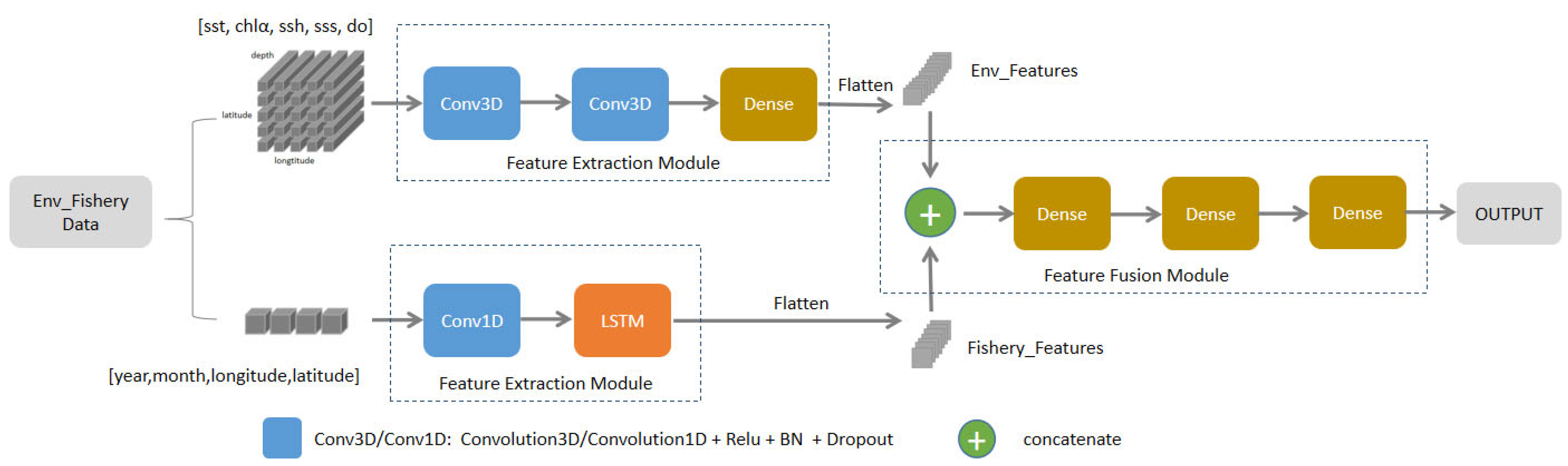
2 improved to more than 0.965. Although the result is better than that of the single neural network, the combined sequence model cannot use specific network models to extract features for different data structures. For example, the LSTM module in the sequence model is good at feature extraction for spatial and temporal factors, but the feature-extraction ability of ocean environment factors is very poor. Therefore, the LSTM module should not be used to extract ocean environment factors.
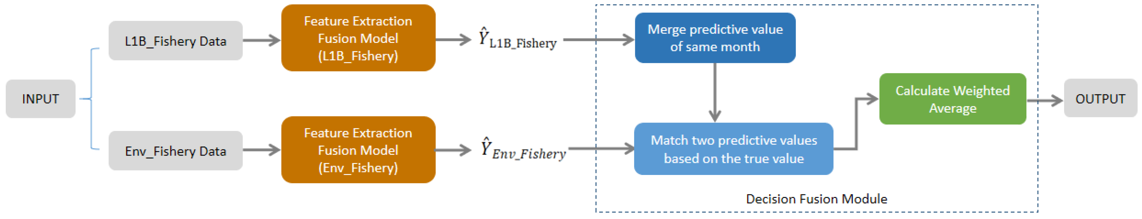
In this paper, for the different structural features of each part of the heterogeneous data, we use the strategy of separate feature extraction and then feature fusion, and we propose the heterogeneous data-feature-extraction model. This model can select the suitable feature-extraction model to fully exploit features for each part of heterogeneous data. The prediction error reduces to 0.02193 and 0.01801 on both datasets, respectively. Then the decision fusion model based on multi-source heterogeneous data feature extraction proposed fuse two datasets of different size and structure, further improving the experiment performance. The mean R2 reaches 0.9901, and the prediction error decreases to 0.01588, while avoiding overfitting, which is significantly better than the experiment results of any single dataset.
Combining the above analysis, the decision fusion model based on multi-source heterogeneous data feature extraction proposed performed outstandingly in the model validation experiment. It has a high fitness to the validation datasets, which is better than other models.

3.3.2. Results Analysis of Generalization Experiments

In order to verify the validity and advancement of the model proposed in the generalization experiment, the CNN–LSTM–BPNN, which performed well (R2 > 0.96) on the model validation experiment of both datasets, is selected for comparison experiments. The results of the comparison experiments are shown in Table 6.
Table 6 shows that the proposed heterogeneous data feature-extraction model performed better in the generalization experiment than in the sequence network CNN–LSTM–BPNN model. On the Env_Fishery datasets, the Feature Extraction Fusion Model reduces the prediction error by 0.6% and improves the R2 by 0.06 compared with the CNN–LSTM–BPNN; on the L1B_Fishery datasets, the feature-extraction fusion model reduces the prediction error by 1% and improves the R2 by 0.07. Then the decision fusion model further reduces the prediction error to 0.07849 and improves the R2 to 0.4237 after the decision fusion of the prediction results of two heterogeneous data feature-extraction models. It shows the best prediction performance in the generalization experiment and significantly better than in any single dataset.
The prediction error of the generalization experiment is only 0.07849, but R2 is equal to 0.4237. It shows that the model has much room for improvement in the fitness of the test datasets. As mentioned in Section 3.2.2, there is still a gap between the generalization experiment prediction results and the high fitness-model-validation-experiment prediction results. Next, we classify the test datasets and their prediction results by month and prediction error to analyze the reasons that affect the further improvement of the generalization experiment performance.
The test datasets used in the generalization experiment is the Northwest Pacific Saury fisheries datasets from 2020. Through the experiments of the proposed models, we can obtain the datasets of CPUE prediction results containing 2603 entries for 8 months (May to December). Referring to the mean prediction error (RMSE = 0.07849), we use a prediction error of 8 ± 2% as the classification criterion to divide the samples of prediction results’ datasets into three classes. Samples with less than a 6% prediction error are high-quality prediction samples (High); samples with a prediction error greater than or equal to 6% but less than or equal to 10% are middle-quality prediction samples (Middle); and samples with prediction errors greater than 10% are low-quality prediction samples (Low).
As shown in Table 7, the total number of samples is listed; the number and proportion of high-, middle-, and low-prediction-quality samples for each month of the test datasets are recorded; and the RMSE of the CPUE value for that month is calculated at the end.
The analysis of Table 7 shows that the high-quality prediction samples account for 55.05% of the overall samples, while the low-quality prediction samples account for only 16.64%. It proves that the proposed model can accurately predict nearly 84% CPUE values of the samples in the test datasets, keeping the errors within 10%. For the low-quality prediction samples, we analyze the reasons of excessive prediction error monthly. Observing Table 7, we can see that there is a high proportion of low-quality prediction samples in May and October, respectively reaching 71.43% and 32.78%, resulting in an above-mean RMSE (0.12256 and 0.009823) for that month. In addition, although the proportion of low-quality prediction samples is low in December, that RMSE is above 0.1, which is also less than ideal.
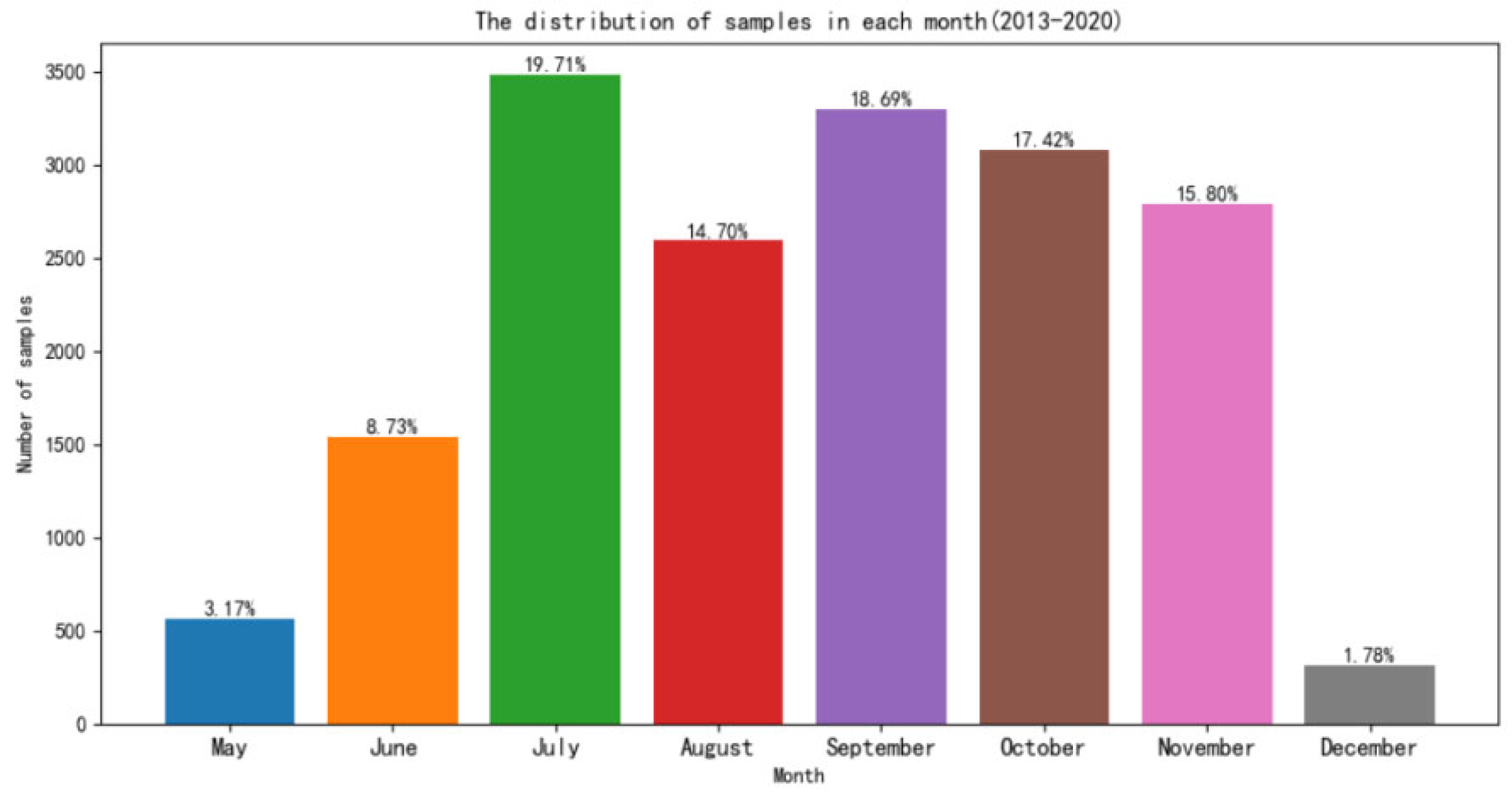
Considering that the peak season of fishing operations is summer and autumn, the number of samples in the fisheries’ datasets is not evenly distributed over the months. The distribution of samples in each month is shown in Figure 11. Because May and December are at the beginning and end of fishing operations each year, the number of samples obtained is very small, accounting for only 3.17% and 1.78%. The December fisheries’ datasets contain only 315 entries in total, while the test datasets contain 115 entries, accounting for more than 1/3 of the total, making December datasets for training and validation even more scarce. Therefore, the uneven distribution of fisheries’ datasets leads to insufficient training in some months. It affects the prediction accuracy of the generalization experiment.
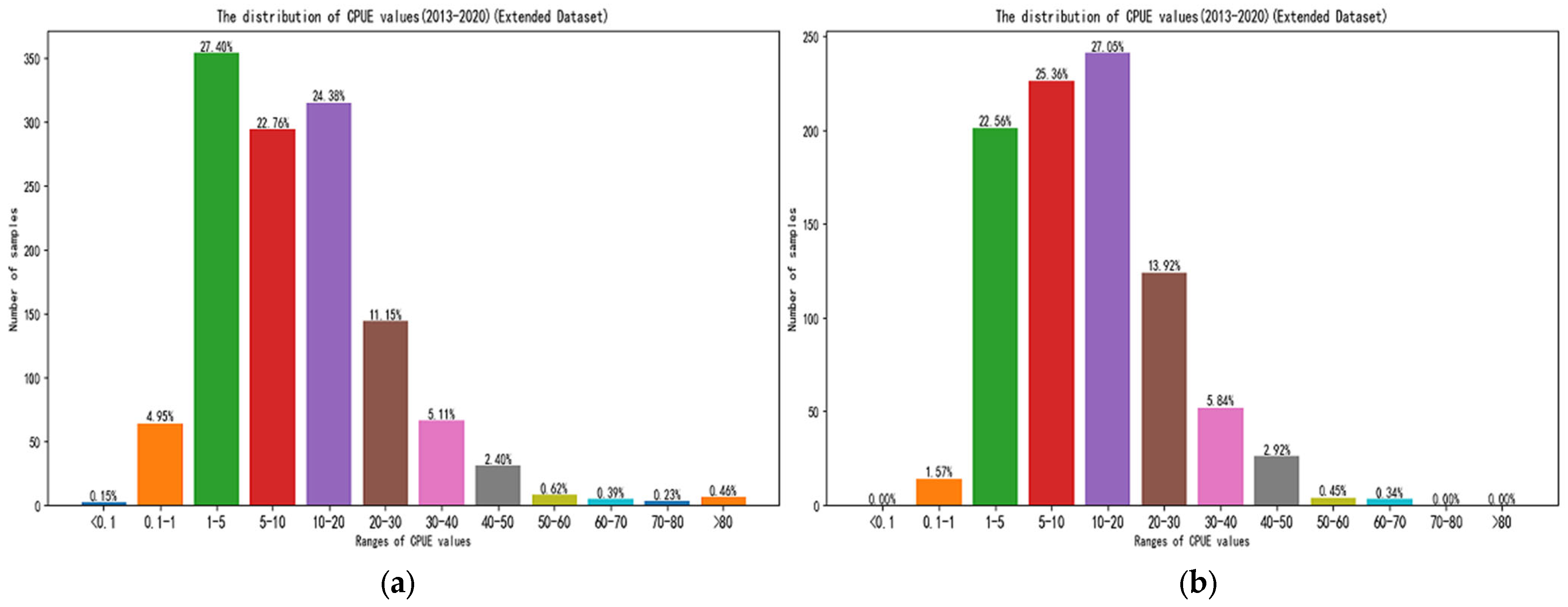
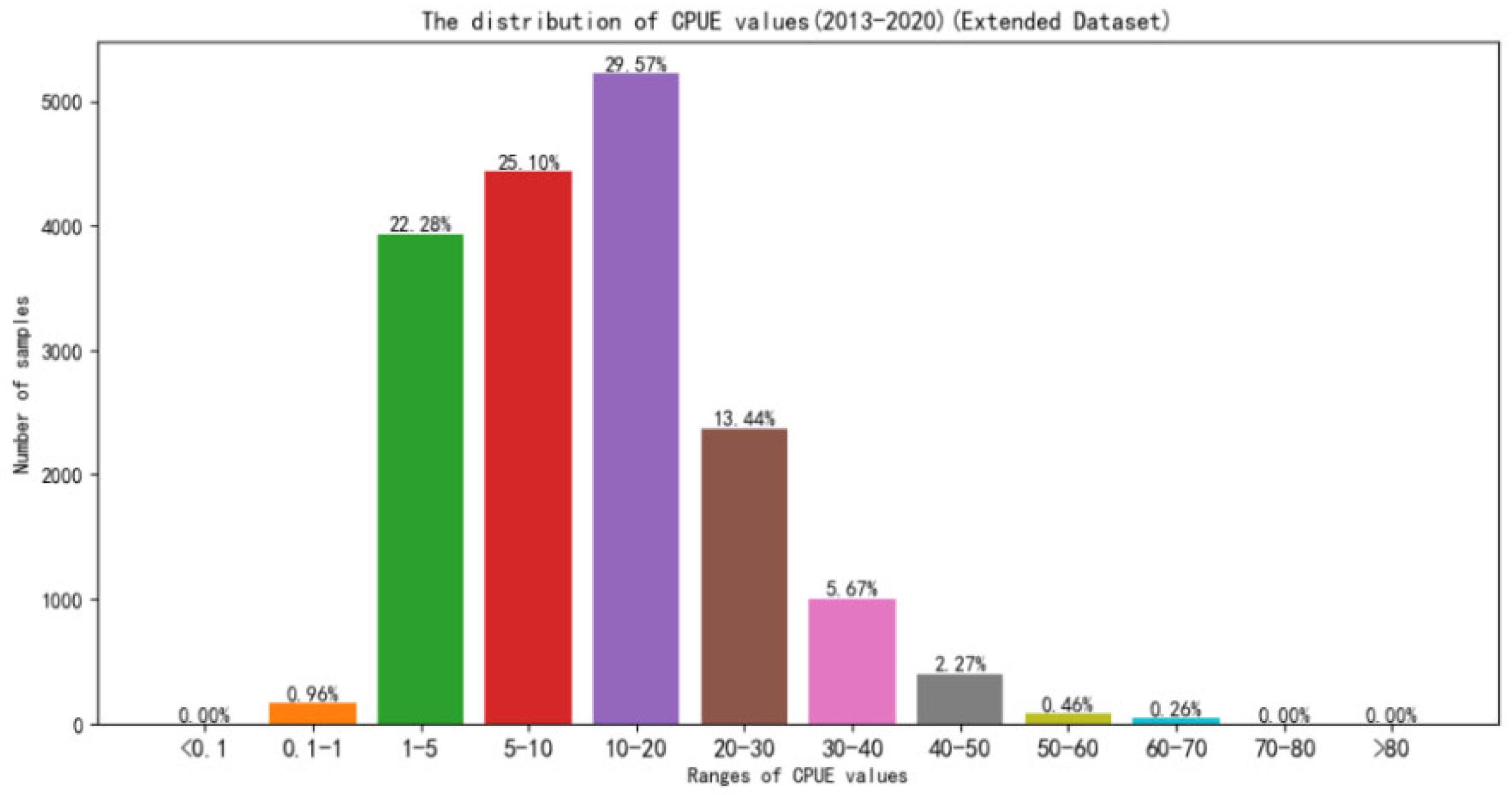
In addition, the uneven distribution of CPUE values also becomes an important reason to affect the prediction accuracy. The distribution of CPUE values after the datasets’ expansion is shown in Figure 12. It can be seen that nearly 80% of the samples of CPUE values are in the low-to-middle level (0.1~20). Only 13.44% of the samples of CPUE values are 20 to 30, and 8.66% of the samples of high CPUE values are above 30.
As shown in 
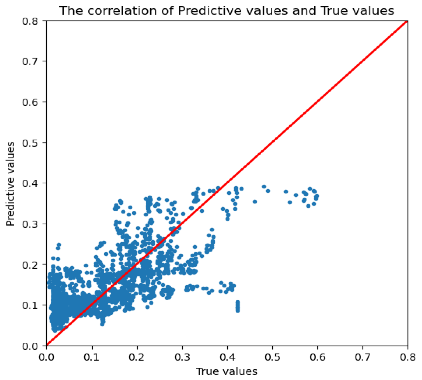
Figure 13, we obtained the correlation of the prediction results of CPUE values and true values of an experiment by using a decision fusion model based on multi-source heterogeneous data feature extraction for generalization experiment. The x-axis in the figure represents the true value of this experiment result, and the y-axis represents the predicted value of this experiment result. If the sample point lies on the y = x function line (red line), it indicates that this predicted value is consistent with its true value, and a sample point below the red line illustrates that the predictive value is lower than the true value. Conversely, it means that the predictive value is higher than the true value. Obviously, for the samples with middle-to-high CPUE values, most of the sample points are below the red line. It illustrates that the uneven distribution of CPUE values affects the training of the model for the samples with medium and high CPUE values. It leads to the poor fitting of the model for the samples of middle and high CPUE values, and its prediction results are low.
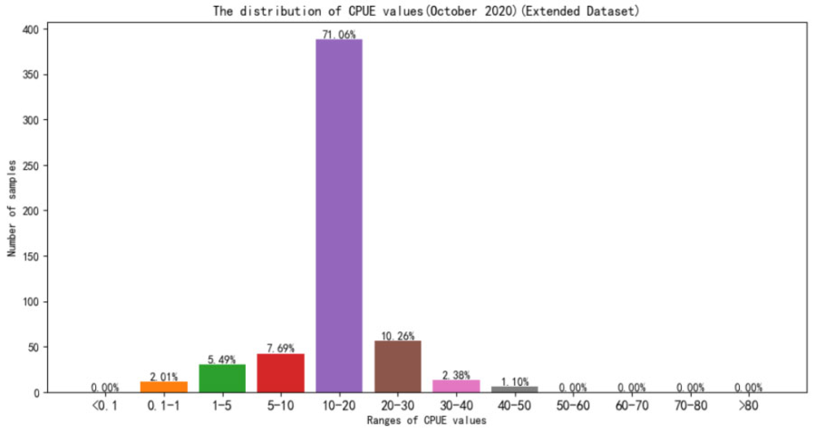
The distribution of CPUE values in October and December on the test datasets are respectively shown in Figure 14 and Figure 15. From the Figure 14, it can be seen that the samples of middle-to-high CPUE values (CPUE > 20) in the October is 13.74%. Although it does not account for a large proportion of the overall, it contains 3.48% samples with high CPUE values (CPUE > 30), accounting for 100% of the samples with high CPUE values in the test datasets. It means that all samples of the high CPUE values in the test datasets are found in October. The reason for the concentration of high CPUE values is related to the peak fishing season in October, when there is a large amount of work, and the quality of the Northwest Pacific Saury is higher than in previous months. Combined with the higher penalty weight given by RMSE to larger prediction error, RMSE is excessively high, nearly 0.1. In addition, 
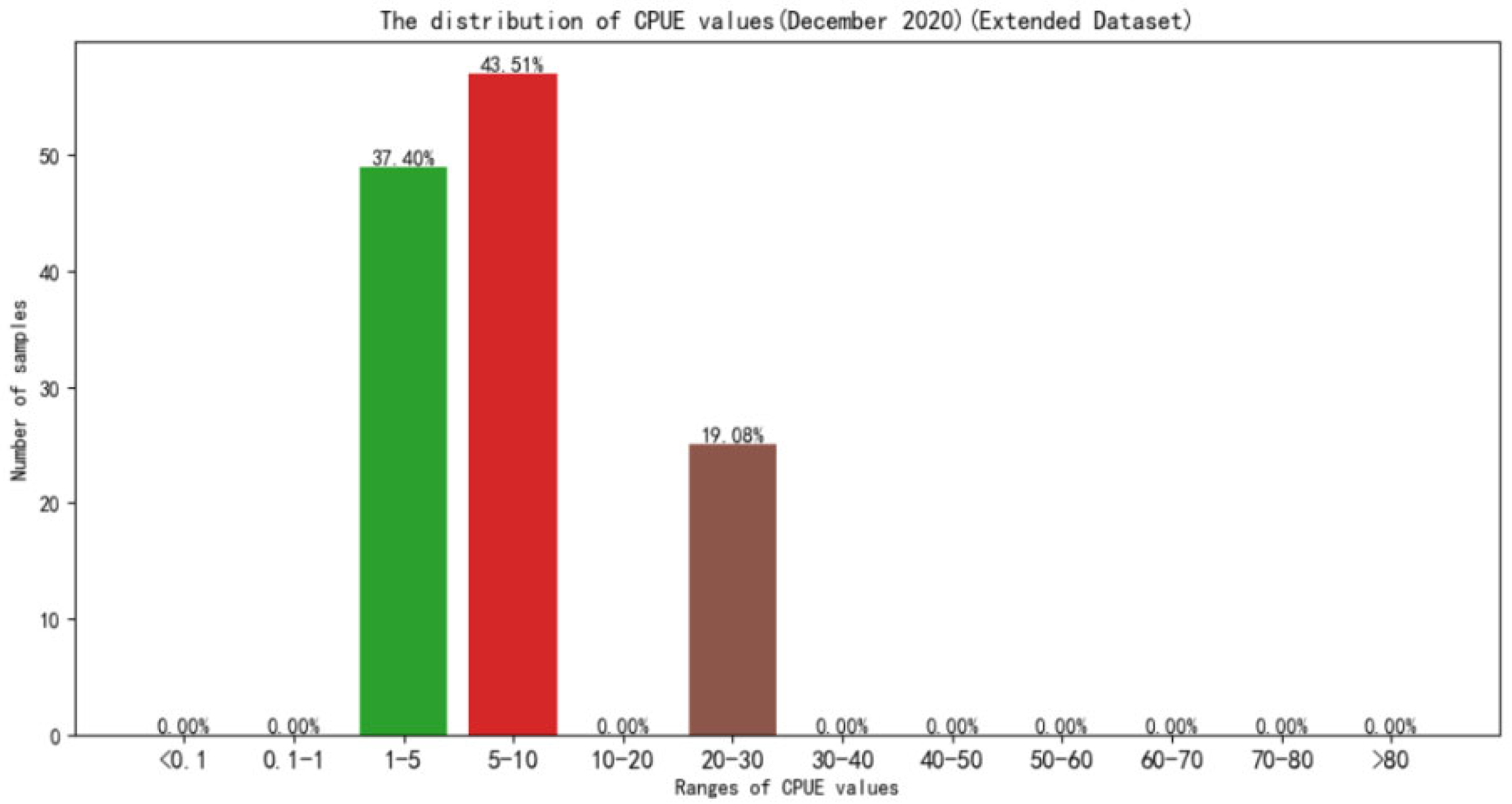
Figure 15 shows that, although the December does not have the effect of high CPUE values, nearly 20% of the samples of the CPUE values are in the 20–30 range. This proportion exceeds the average of the fisheries datasets. Coupled with too little data of December fisheries datasets used to train the model, the training model is under-fitting, resulting in an RMSE of more than 0.1.
In summary, the proposed decision fusion model based on multi-source heterogeneous data feature extraction performed excellently in the generalization experiment. It fit most of the data well and kept the overall prediction error at less than 8%, which is better than other models. However, due to the unevenness of fisheries’ data in the distribution of month and CPUE value, the prediction accuracy is not ideal for samples from months with less data and samples of middle-to-high CPUE values. It limits the further improvement of the model prediction accuracy in the generalization experiment.

4. Discussion

Overall, the decision fusion model based on the feature extraction of multi-source heterogeneous data proposed in this paper consists of three parts: feature extraction, feature-level fusion, and decision-level fusion. Firstly, it selects a suitable feature-extraction model to extract features separately according to the structural features of each part of the heterogeneous data: 1D-CNN and LSTM are used to deeply explore spatial and temporal factors’ features in fisheries’ data; the powerful spatial feature-extraction capability of the 3D-CNN is used to extract high-dimensional ocean environment factor features containing the surrounding environment information; and a 1D-CNN and BP neural network with residual structure is used to fully extract features of larger-scale multi-spectral bands’ factor data. Then the model fully fuses the features through a three-layer full-connection network. Finally, the feature-fusion results of the two datasets are fused by the optimal weighted average algorithm of the decision fusion module to obtain the prediction results.
To illustrate the effectiveness of the proposed method in this paper, a series of experiments were conducted. In Section 3.3.1, we covered comparison experiments that we conducted between the existing typical habitat-prediction methods [10,11,12,13,21,22,23,24,25] and the feature-fusion model proposed in this paper, using single-source data, respectively. The RMSE of the feature-fusion model proposed in this paper is 0.02193 and 0.01801 for the two single-source inputs, and the R2 is above 0.98. It is better than the models in the existing literature, proving the effectiveness of the proposed feature fusion-model in this paper. On this basis, we used multi-source heterogeneous data sources to build a decision fusion model and obtain optimal results, with a mean R2 of 0.9901 and the error reduced to 0.01588, while avoiding overfitting. It further demonstrates the effectiveness and advancement of the proposed decision fusion model of habitat prediction with multi-source heterogeneous data in this paper compared to the single-source data model used in the previous literature.
By examining the previous literature, we find that research in the field of habitat prediction is gradually shifting from traditional mathematical models to machine-learning models, which can be adapted to larger-scale remote-sensing data processing and prediction [14]. Most of the current research methods in this field that achieve good prediction results use single-source sequential networks, which are generally better than traditional machine-learning models such as SVM and RF. For example, Yuan [26] used a sequence fusion deep network model to predict the albacore tuna habitat in the South Pacific Ocean and obtained the prediction result with an average error of 0.028. Based on this, we propose a multilevel fusion network model based on multi-source heterogeneous data that can deeply explore the spatial and temporal factors features in fisheries’ data by using the powerful spatial feature-extraction ability of the improved CNN and combining with the LSTM. The comparative analysis of the habitat-prediction methods shows that the method proposed in this paper obtains the better performance, with the prediction error reduced to 0.016, proving the advancement and effectiveness of the proposed model in this paper.
In addition, in a previous generalization experiment in the literature, Wei [27] obtained prediction results with an average error of 0.105 by using single-source product-level data and the BP network model in the Pacific Northwest squid habitat, and this result is better than most previous results in the literature. In Section 3.3.2, the multilevel fusion network model based on multi-source heterogeneous inputs proposed in this paper reduces the prediction error to 0.079, which significantly reduces the prediction error in generalization experiments. It further proves the effectiveness of the method proposed in this paper in generalization experiments.
Therefore, based on the limitations of single-source data, this paper innovatively proposes to take advantage of the multi-source heterogeneous data of product-level remote-sensing data and L1B original multi-spectral remote-sensing data to build a fusion network. It can fully exploit and deeply fuse the data features of different structures and sizes, solving the problem of the ineffective fusion of multi-source heterogeneous data, and it achieves better prediction of habitat. The experiment results demonstrate that the proposed method can effectively improve the accuracy of habitat prediction compared with the single-source sequence network model in the existing literature, thus proving the feasibility of using multi-source remote-sensing data for fishery prediction and innovatively expanding the range of data selection for research in this field. It can be said that the method proposed in this paper provides new ideas for future research in the field of habitat prediction.

5. Conclusions

Considering the problem that the product-level environment-factor remote-sensing data used in the previous habitat prediction may lose some potential habitat features in the inversion process, eleven original MODIS L1B bands related to ocean environment factors were used to enrich the environment-factor-feature datasets. Moreover, we obtained two datasets with different structures and sizes by matching with the fisheries’ datasets. For the multi-source heterogeneous datasets, this experiment innovatively proposes a decision fusion model based on the feature extraction of multi-source heterogeneous data, as such a model solves the problem of ineffective fusion of multi-source heterogeneous data and fully exploits and utilizes the features of remote-sensing fishery data with different data structures and sizes. Finally, weed obtain more accurate and effective habitat-prediction results.
However, the unevenness of fisheries’ data in the distribution of month and CPUE value makes the prediction accuracy of the datasets with less data in months and the datasets with higher CPUE values in months less satisfactory, thus limiting the further improvement of the model prediction effect in the generalization experiment. In addition, the selection criteria of the product-level ocean-environment-factor data are based on previous habitat-prediction research. Five common environment factors with convenient access and mature technology are selected. However, these selection criteria lack a targeted analysis of the correlation between the Pacific Saury habits and different ocean environment factors; MODIS L1B bands’ factor data are obtained by directly selecting multi-spectral bands related to ocean environment factors. This method lacks the analysis and comparison of information in other bands. Because of the richness and relevance of the information carried by different bands, it is also possible for feature information related to habitat prediction in the remaining bands to exist.
Therefore, based on this experimental study, the next step should be to conduct more analyses and comparison experiments on the rationality of the selection of environment factors to ensure the strong correlation between environment factors and the formation of habitat. In addition, the targeted processing of the fisheries’ datasets should be strengthened to reduce the effect of the uneven distribution of month and CPUE values. Finally, the model should be optimized to further improve the model’s prediction accuracy in the generalization experiment by using an attention mechanism, because it can enhance training and feature extraction of some data.

Author Contributions

Conceptualization, Y.H.; methodology, Y.H. and J.G.; software, Y.H. and J.G.; validation, Y.H., J.G. and Z.M.; formal analysis, Y.H. and J.G.; investigation, J.W.; resources, Y.H., J.G. and R.Z.; data curation, J.G; writing—original draft preparation, Y.H. and J.G.; writing—review and editing, Y.H., J.G., Z.M. and Y.Z.; visualization, Y.H. and J.G.; supervision, Y.H., Z.M. and Z.H.; project administration, H.P. All authors have read and agreed to the published version of the manuscript.

Funding

This work was supported by the National Key R&D Program of China, Grant Number 2019YFD0900805, and National Natural Science Foundation of China (Grant No. 42176175).

Data Availability Statement

The fisheries data used in this study were provided by the Northwest Pacific Saury of Technical Group of Shanghai Ocean University. The data are not publicly available due to restrictions of privacy and law. The product-level environment-factor remote-sensing data presented in this study are available in the Copernicus Marine Service Web (https://marine.copernicus.eu/) (accessed on 16 April 2022). The MODIS L1B original remote-sensing data presented in this study are available in the data-download web provided by NASA (https://ladsweb.modaps.eosdis.nasa.gov/).

Acknowledgments

We would like to thank Chuanxiang Hua’s research group of the Northwest Pacific Saury at Shanghai Ocean University for providing fisheries datasets for this experiment so that our study could be successfully completed.

Conflicts of Interest

The authors declare no conflict of interest.

References

  1. Shan, J.H.; Han, S.X.; Fan, W.; Zhou, S.F. Saury Resource and Fishing Grounds in the Northwest Pacific. Mar. Fish. 2004, 26, 61–65. [Google Scholar]
  2. Sun, M.C.; Ye, X.C.; Zhang, J.; Qian, W.G. Exploration of Saury in the Northwest Pacific. Mar. Fish. 2003, 25, 112–115. [Google Scholar]
  3. Zavolokin, A. Priority Species [EB/OL]. [2018-06-09]. Available online: https://www.npfc.int/priority-species (accessed on 6 February 2022).
  4. Meng, L.W. Study on Fishery Forecast Research of Cololabis Saira in North Pacific Ocean Based on Habitat Model. Master’s Thesis, Shanghai Ocean University, Shanghai, China, 2017. [Google Scholar]
  5. Hua, C.; Zhu, Q.; Shi, Y.; Liu, Y. Comparative analysis of CPUE standardization of Chinese Pacific saury (Cololabis saira) fishery based on GLM and GAM. Acta Oceanol. Sinica 2019, 38, 100–110. [Google Scholar] [CrossRef]
  6. Choudhury, S.B.; Jena, B.; Rao, M.V.; Rao, K.H.; Somvanshi, V.S.; Gulati, D.K.; Sahu, S.K. Validation of integrated potential fishing zone (IPFZ) forecast using satellite based chlorophyll and sea surface temperature along the east coast of India. Int. J. Remote Sens. 2007, 28, 2683–2693. [Google Scholar] [CrossRef]
  7. Yan, L.; Zhu, Q.C.; Zhang, Y.; Shang, L.L. Fishing ground distribution of saury and its correlation with SST in the Northern Pacific high sea in 2010. J. Shanghai Ocean. Univ. 2012, 21, 609–615. [Google Scholar]
  8. Hua, C.X.; Zhu, Q.C.; Xu, W.; Song, L.M. Review of the life history, resources and fishing grounds of the Pacific saury in the North Pacific Ocean. J. Fish. Sci. China 2019, 26, 811–821. [Google Scholar]
  9. Tian, Y.J.; Akamine, T.; Suda, M. Modeling the influence of oceanic-climatic changes on the dynamics of Pacific saury in the northwestern Pacific using a life cycle model. Fish. Oceanogr. 2004, 13, 125–137. [Google Scholar] [CrossRef]
  10. Liu, Y.; Hua, C.X. Forecasting Pacific saury (Cololabis saira) fisheries based on GAM and weighted analysis in the northwest Pacific. J. Fish. Sci. China 2021, 28, 888–895. [Google Scholar]
  11. Chen, X.Z.; Fan, W.; Cui, X.S.; Zhou, W.; Tang, F. Fishing ground forecasting of Thunnus alalunga in Indian Ocean based on random forest. Acta Oceanol. Sinica 2013, 35, 158–164. [Google Scholar]
  12. Mugo, R.; Saitoh, S.-I. Ensemble Modelling of Skipjack Tuna (Katsuwonus pelamis) Habitats in the Western North Pacific Using Satellite Remotely Sensed Data; a Comparative Analysis Using Machine-Learning Models. Remote Sens. 2020, 12, 2591. [Google Scholar] [CrossRef]
  13. Wang, J.T.; Gao, F.; Lei, L.; Guan, W.J.; Chen, X.J. Impacts of temporal and spatial scale as well as environmental data on fishery forecasting models for Illex argentinus in the southwest Atlantic. J. Fish. Sci. China 2015, 22, 1007–1014. [Google Scholar]
  14. Cavieses Núñez, R.A.; Ojeda Ruiz de la Peña, M.Á.; Flores Irigollen, A.; Rodríguez Rodríguez, M. Deep learning models for the prediction of small-scale fisheries catches: Finfish fishery in the region of “Bahía Magadalena-Almejas”. ICES J. Mar. Sci. 2018, 75, 2088–2096. [Google Scholar] [CrossRef]
  15. Yuan, H.C.; Zhang, S.; Chen, G.Q.; Liu, H. Fishing ground forecast model of albacore tuna based on fully convolutional networks in the South Pacific. Jiangsu J. Agr. Sci. 2020, 36, 423–429. [Google Scholar]
  16. Yuan, H.C.; Zhang, S.; Chen, G.Q.; Liu, H. Fishery forecasting in the fishing ground based on dual-modal deep learning model. Jiangsu J. Agr. Sci. 2021, 37, 435–442. [Google Scholar]
  17. Zhang, X.M.; Zhu, C.Q.; Hua, C.X. Fishing ground distribution of saury and its correlation with marine environment factors in the Northern Parcific high sea in 2013. J. Shanghai Ocean. Univ. 2015, 24, 773–781. [Google Scholar]
  18. Zhu, H.P. Construction of Fishing Ground Forecast Model of Ommastrephes bartramii in Northwest Pacific Based on Convolutional Neural Network. Master’s Thesis, Shanghai Ocean University, Shanghai, China, 2021. [Google Scholar]
  19. Mammel, M.; Naimullah, M.; Vayghan, A.H.; Hsu, J.; Lee, M.A.; Wu, J.H.; Wang, Y.C.; Lan, K.W. Variability in the Spatiotemporal Distribution Patterns of Greater Amberjack in Response to Environmental Factors in the Taiwan Strait Using Remote Sensing Data. Remote Sens. 2022, 14, 2932. [Google Scholar] [CrossRef]
  20. Yu, W.; Chen, X.J.; Yi, Q.; Chen, Y. Spatio-temporal distributions and habitat hot spots of the winter-spring cohort of neon flying squid Ommastrephes bartramii in relation to oceanographic conditions in the Northwest Pacific Ocean. Fish. Res. 2016, 175, 103–115. [Google Scholar] [CrossRef]
  21. Walsh, W.A.; Kleiber, P. Generalized additive model and regression tree analyses of blue shark (Prionace glauca) catch rates by the Hawaii-based commercial longline fishery. Fish. Res. 2001, 53, 115–131. [Google Scholar] [CrossRef]
  22. Giri, S.; Purkayastha, S.; Hazra, S.; Chanda, A.; Das, I.; Das, S. Prediction of monthly Hilsa (Tenualosa ilisha) catch in the Northern Bay of Bengal using Bayesian structural time series model. Reg. Stud. Mar. Sci. 2020, 39, 101456. [Google Scholar] [CrossRef]
  23. Wang, J.; Chen, X.; Staples, K.W.; Chen, Y. The skipjack tuna fishery in the west-central Pacific Ocean: Applying neural networks to detect habitat preferences. Fish. Sci. 2018, 84, 309–321. [Google Scholar] [CrossRef]
  24. Wang, J.; Yu, W.; Chen, X.; Lei, L.; Chen, Y. Detection of potential fishing zones for neon flying squid based on remote-sensing data in the Northwest Pacific Ocean using an artificial neural network. Int. J. Remote Sens. 2015, 36, 3317–3330. [Google Scholar] [CrossRef]
  25. Kim, M.; Yang, H.; Kim, J. Sea Surface Temperature and High Water Temperature Occurrence Prediction Using a Long Short-Term Memory Model. Remote Sens. 2020, 12, 3654. [Google Scholar] [CrossRef]
  26. Yuan, H.C.; Chen, C.H. Prediction of Thunnus alalunga fishery based on fusion deep learning model. Fish. Mod. 2019, 46, 74–81. [Google Scholar]
  27. Wei, L.; Chen, X.J.; Lei, L.; Wang, J.T. Comparative study on the forecasting models of squid fishing ground in the northwest Pacific Ocean based on BP artificial neural network. J. Shanghai Ocean. Univ. 2017, 26, 450–457. [Google Scholar]
Figure 1. (a) The distribution of CPUE values of the fisheries’ datasets. (b) The distribution of CPUE values of the fisheries’ datasets after deletion of outliers.
Remotesensing 14 05061 g001
Figure 2. Example of data expansion in fisheries’ datasets.
Remotesensing 14 05061 g002
Figure 3. Distribution of Chlα and SST data for a month in the study area.
Remotesensing 14 05061 g003
Figure 4. (a) A region of visible-light band image. (b) The image after Normalized Detection Index processed.
Remotesensing 14 05061 g004
Figure 5. Env_Fishery data structure.
Remotesensing 14 05061 g005
Figure 6. L1B_Fishery data structure.
Remotesensing 14 05061 g006
Figure 7. The heterogeneous data feature-extraction model structure with Env_Fishery data as input.
Remotesensing 14 05061 g007
Figure 8. The heterogeneous data feature-extraction model’s structure with L1B_Fishery data as input.
Remotesensing 14 05061 g008
Figure 9. The structure of the decision fusion model based on multi-source heterogeneous data feature extraction with L1B_Fishery and Env_Fishery datasets as input.
Remotesensing 14 05061 g009
Figure 10. RMSE change curves under different weight ratios in model validation experiment and generalization experiment.
Remotesensing 14 05061 g010
Figure 11. The distribution of samples of fisheries’ datasets in each month in 2013~2020.
Remotesensing 14 05061 g011
Figure 12. The distribution of CPUE values of fisheries datasets after the dataset’s expansion from approximately 2013 to 2020.
Remotesensing 14 05061 g012
Figure 13. The correlation of the prediction results of CPUE values and true values.
Remotesensing 14 05061 g013
Figure 14. The distribution of CPUE values of samples in test datasets in October 2020.
Remotesensing 14 05061 g014
Figure 15. The distribution of CPUE values of samples in test datasets in December 2020.
Remotesensing 14 05061 g015
Table 1. Comparison and analysis of experiment results of the filling in of missing values.
MethodsMSEMAER2Advantages and Disadvantages
Space–Time Factor Mean Algorithm0.04730.12070.9978It is a simple method but poor effect in the face of continuous missing values
K-Nearest-Neighbors Algorithm0.07650.18640.9965Suitable, but with large errors
Random Forest Algorithm0.02610.11240.9988Effective in the face of continuous missing value, but the algorithm takes too much time
Table 2. Experiment results comparing the number of different CNN convolution kernels and LSTM block neurons.
The Number of CNN Convolution KernelsThe Number of LSTM Block NeuronsRMSE (Val)R2 (Val)
641000.035240.9506
1281000.031630.9589
1281200.027440.9700
2561500.021980.9808
5121500.021240.9832
5122000.020910.9847
Table 3. The model-validation-experiment and generalization-experiment results of two heterogeneous data feature-extraction models with L1B_Fishery and Env_Fishery datasets as input.
Input DatasetsModel Validation ExperimentGeneralization Experiment
RMSE (Val)R2 (Val)RMSE (Test)R2 (Test)
L1B_Fishery0.019440.98560.086190.3382
L1B_Fishery0.018100.98750.085680.3460
L1B_Fishery0.016490.98960.084560.3631
Average (L1B_Fishery)0.018010.98760.085480.3491
Env_Fishery0.022080.98060.081860.3733
Env_Fishery0.021980.98080.081710.3755
Env_Fishery0.021740.98120.081250.3827
Average (Env_Fishery)0.021930.98090.081610.3772
Table 4. The average performance of the nine-times decision fusion results of same kind of experiments with different weight ratios.
ω L 1 B _ F i s h e r y   : ω E n v _ F i s h e r y Model Validation ExperimentGeneralization Experiment
RMSE (Val)R2 (Val)RMSE (Test)R2 (Test)
1:90.020370.98350.080470.3944
2:80.018970.98570.079590.4076
3:70.017780.98740.078960.4169
4:60.016840.98870.078590.4223
5:50.016200.98960.078490.4237
6:40.015880.99010.078660.4212
7:30.015920.98990.079100.4148
8:20.016300.98940.079800.4043
9:10.017000.98850.080760.3900
Table 5. Comparison of the results of different models in the model validation experiment.
Experiment ModelExperiment DatasetsRMSE (Val)R2 (Val)
LREnv_Fishery0.138020.2422
BREnv_Fishery0.138020.2422
SVREnv_Fishery0.084600.7152
RTEnv_Fishery0.045900.9161
RFEnv_Fishery0.035730.9492
BPNNEnv_Fishery0.040980.9332
BPNNL1B_Fishery0.031550.9639
CNNEnv_Fishery0.043470.9248
CNNL1B_Fishery0.041790.9359
LSTMEnv_Fishery0.040110.9360
LSTML1B_Fishery0.032870.9604
CNN–LSTM–BPNNEnv_Fishery0.029630.9651
CNN–LSTM–BPNNL1B_Fishery0.023610.9795
Feature-Extraction Fusion ModelEnv_Fishery0.021930.9809
Feature-Extraction Fusion ModelL1B_Fishery0.018010.9876
Decision Fusion ModelEnv_Fishery + L1B_Fishery0.015880.9901
Table 6. Results of comparison between different models in the generalization experiment.
Experiment ModelExperiment DatasetsRMSE (Val)R2 (Val)
CNN–LSTM–BPNNEnv_Fishery0.087380.3184
CNN–LSTM–BPNNL1B_Fishery0.095610.2756
Feature-Extraction Fusion ModelEnv_Fishery0.081610.3772
Feature-Extraction Fusion ModelL1B_Fishery0.085480.3491
Decision Fusion ModelEnv_Fishery + L1B_Fishery0.078490.4237
Table 7. Total number of samples; number and proportion of high-, middle-, and low-prediction-quality samples; and RMSE for each month of the test datasets are recorded in this table.
MonthAllHighMiddleLowH_PercentM_PercentL_PercentRMSE
5708125011.43%17.14%71.43%0.12256
6205130433263.42%20.97%15.61%0.06795
7550 3342001660.73%36.36%2.91%0.05740
81919596049.74%50.26%00.06085
95012731725654.49%34.33%11.18%0.06999
1054625611117946.89%20.33%32.78%0.09823
11425267788062.83%18.35%18.82%0.07001
1211570252060.87%21.74%17.39%0.10715
Sum2603143373743355.05%28.31%16.64%0.07849
Publisher’s Note: MDPI stays neutral with regard to jurisdictional claims in published maps and institutional affiliations.

