Article

CNN-Enhanced Heterogeneous Graph Convolutional Network: Inferring Land Use from Land Cover with a Case Study of Park Segmentation

1
Aerospace Information Research Institute (AIR), Chinese Academy of Sciences (CAS), Beijing 100094, China
2
University of Chinese Academy of Sciences (UCAS), Beijing 100049, China
*
Author to whom correspondence should be addressed.
Remote Sens. 2022, 14(19), 5027; https://doi.org/10.3390/rs14195027
Submission received: 26 August 2022 / Revised: 29 September 2022 / Accepted: 3 October 2022 / Published: 9 October 2022
(This article belongs to the Topic Advances in Environmental Remote Sensing)

Abstract

:
Land use segmentation is a fundamental yet challenging task in remote sensing. Most current methods mainly take images as input and sometimes cannot achieve satisfactory results due to limited information. Inspired by the inherent relations between land cover and land use, we investigate land use segmentation using additional land cover data. The topological relations among land cover objects are beneficial for bridging the semantic gap between land cover and land use. Specifically, these relations are usually depicted by a geo-object-based graph structure. Deep convolutional neural networks (CNNs) are capable of extracting local patterns but fail to efficiently explore topological relations. In contrast, contextual relations among objects can be easily captured by graph convolutional networks (GCNs). In this study, we integrated CNNs and GCNs and proposed the CNN-enhanced HEterogeneous Graph Convolutional Network (CHeGCN) to incorporate local spectral-spatial features and long-range dependencies. We represent topological relations by heterogeneous graphs which are constructed with images and land cover data. Afterwards, we employed GCNs to build topological relations by graph reasoning. Finally, we fused CNN and GCN features to accomplish the inference from land cover to land use. Compared with other homogeneous graph-based models, the land cover data provide more sufficient information for graph reasoning. The proposed method can achieve the transformation from land cover to land use. Extensive experiments showed the competitive performance of CHeGCN and demonstrated the positive effects of land cover data. On the IoU metric over two datasets, CHeGCN outperforms CNNs and GCNs by nearly 3.5% and 5%, respectively. In contrast to homogeneous graphs, heterogeneous graphs have an IoU improvement of approximately 2.5% in the ablation experiments. Furthermore, the generated visualizations help explore the underlying mechanism of CHeGCN. It is worth noting that CHeGCN can be easily degenerated to scenarios where no land cover information is available and achieves satisfactory performance.

1. Introduction

Land use information is critical for understanding complex human–environment relationships and promoting human socioeconomic development, such as environmental change [1], ecosystem deterioration [2], and urban planning [3]. There is a tremendous demand for land use mapping for sustainable urban development in this era of rapid urbanization and population growth. However, land use, in contrast to land cover, is more difficult to distinguish. Land cover can be directly identified from images as it relates to the physical characteristics of the ground surface [4], while land use reflects the socio-economic activities that take place on that surface. A land use unit may comprise a variety of diverse land cover types, resulting in dramatic differences in spatial arrangement and spectral characteristics, even in a homogeneous land use region [5]. Thus, it is challenging to obtain reliable land use segmentation using low-level image features, such as spectral and textural features. Meanwhile, information about land use is implicitly provided as patterns or high-level semantic functions in very fine spatial resolution (VFSR) satellite images [6]. Hence, it is essential to extract high-level semantic features from detailed images for accurate land use segmentation.
The topological relations among land cover elements are beneficial for narrowing the semantic gap between land cover and land use [7,8,9]. Topological relations can describe the complicated spatial configuration of land cover objects, which are beneficial for land use identification. This assumption is built on the fact that land use parcels with similar structures tend to possess similar functional attributes [5]. From another perspective, accurate land use segmentation necessitates a thorough understanding of complex urban structures. This structure is a global perception of urban areas, which is built on the long-range dependencies of land cover units. According to the perceptual organization theory, humans group visual objects together to recognize the visual as a whole, where topological relations play an important role in the grouping process.
The positive effects of topological relations can be illustrated by the application of urban park segmentation. Urban parks (hereinafter referred to as parks) are designated areas of natural, semi-natural, or planted space inside cities for human recreation. There are usually multiple land cover types inside a park unit, such as water, buildings, and forest. Thus, the spectral feature distribution of park pixels is irregular and difficult to distinguish. For instance, a building area in a park is easily recognized as non-park because most buildings do not appear in parks. Land cover data are advantageous for solving this problem, as topological relations can be better depicted. For example, a building surrounded by forests is more likely to belong to a park than one surrounded by buildings. As a result, land use segmentation can be further improved by the topological relation inference using land cover data. Meanwhile, land cover classification is one of the most fundamental tasks in remote sensing [10]. There are many well-known public land cover products available, such as GlobeLand30 [11], Finer Resolution Observation and Monitoring of Global Land Cover (FROM-GLC) [12], and ESA’s Land Cover Climate Change Initiative (LC-CCI). Therefore, an appealing idea is to use land cover to support land use segmentation, and models capable of effectively extracting topological relationships are required.
In recent decades, many investigations have been conducted to improve the accuracy of land use segmentation. These approaches can be generally divided into two categories regarding the use of spatial information: grid-based and object-based. Grid-based algorithms learn image representation from regular regions, and the most basic strategy is to use only spectral characteristics for pixel-wise segmentation. Researchers have tried to increase the size of grids to get spatial context features since pixel-wise methods fail to describe the spatial structure of land use. The most successful design among them are deep CNNs, as CNNs provide a powerful framework for local pattern modeling by end-to-end and hierarchical learning. Many attempts have been made to better exploit spatial information. Dilated convolutions are exploited to enlarge receptive fields [13]. Local features are enhanced with a global context vector obtained by global pooling [14]. A pyramid pooling module was employed to collect semantic features [15,16], and on this basis, the atrous special pyramid pooling (ASPP) further incorporates the atrous algorithm [17,18,19,20]. It is worth mentioning that the use of spatial context boosts models’ performance and robustness. Thus, CNNs, such as fully convolutional network (FCN) [21], U-net [22], pyramid scene parsing network (PSPNet) [15], and DeepLabv3 [19] have achieved outstanding results in semantic segmentation. However, these models are highly inefficient in describing long-distance relationships because they are composed of the local operations of convolution and pooling [23,24].
It is preferable to depict relationships between objects rather than regular grids (the comparison can be seen in Figure 1). On the one hand, interregional dependencies are of significantly longer range than those represented by local convolutions [23]. On the other hand, objects and regions are of arbitrary shape in the real world, and object-based methods are more capable of describing the “reality” of human perception than pixel-level approaches [25]. Furthermore, object-based techniques are more ideal for expressing topological relations among land cover objects inside a land use parcel, which, as mentioned before, is extremely beneficial for bridging the semantic gap between land cover and land use. As previous deep learning models are prepared for Euclidean data, complex topological relations among land cover objects are frequently neglected.
It is natural to consider graphs to explore relationships, because images can be easily converted into graphs with vertices and edges indicating image regions and their similarities. Graphs are a widely used data structure as well as a universal language for describing complex systems, and Euclidean data such as images (2D grids) can be regarded as instances of graphs. Graphs, which focus on relationships among objects rather than the attributes of individual objects [26], have shown great expressive power in various domains, including social science [27], protein–protein interaction networks [28], and network biology [29]. Subsequently, context modeling is typically postulated as an inference issue on graphs [30]. In practice, the process of relation reasoning, i.e., context modeling, is realized by the aggregation of node information. The aggregation process depends on the graph structure, which is dominated by the topological relationships of geo-objects. Finally, a land use segmentation problem is converted into a node classification problem.
However, most current models are built on homogeneous graphs and fail to fully employ the rich semantic information of heterogeneous data. Recently, GCNs [31] have received increasing attention for their ability to aggregate information by generalizing convolutions to graph-structure data. By employing GCNs on graphs transformed from images, relations among objects can be explicitly inferred along graph edges, and spatial structures can be better portrayed. For example, GCNs are used to model contextual structures in hyperspectral image classification problems [32,33,34,35]. In detail, GCNs are employed through graph reprojection [23], in which vertex features are projected back to grid space based on region assignments. Then, the projected features are integrated (using operations such as addition) into the CNN feature maps. As mentioned above, it is suggested to accomplish land use segmentation with land cover data. However, these homogeneous graph-based approaches are severely limited in their ability to merge additional data. For instance, a co-occurrence matrix of node classes [36] is employed in an implicit and inefficient way, and the use of coarse prediction maps [37] ignores inter-class relationships and treats nodes of different classes equally.
Heterogeneous graphs [38] are introduced to solve the aforementioned issues, which can appropriately infer land use from land cover. In a heterogeneous graph, the total number of node types and edge types is greater than two, whereas there is only one node type and one edge type in a homogeneous graph (see Figure 1 for the difference).This work [38] fully exploits the heterogeneity and rich semantic information embedded in the multiple node and edge types by using hierarchical attention, which consists of node-level and semantic-level attention. Specifically, the node and edge types are taken into consideration when aggregating features. Heterogeneous graphs are experts in portraying complex relationships among various classes of nodes. Thus, heterogeneous graph-based methods can better mine topological relations among different land cover nodes.
Our model is proposed based on heterogeneous graphs to bridge the semantic gap between land cover and land use. Specifically, in the case of park segmentation, there are m node types and m ( m + 1 ) 2 edge types, where m denotes the number of land cover types. Thus, we can build heterogeneous graphs with land cover data. It makes sense to define different edge calculation functions among the nodes of different land cover classes. For instance, reducing weights between road and forest objects is beneficial given that roads frequently appear outside parks. Moreover, the parameters of class-specific edge calculation functions are automatically learned, making the relation inference more adaptive. Similarly to the feature fusion framework [32,39], we integrate CNNs and our heterogeneous graph-based model to derive long-distance relationships among objects while preserving spatial details, since the shallow features of CNNs retain more spatial information. To this end, we propose the CNN-enhanced HEterogeneous Graph Convolutional Network(CHeGCN) for land use segmentation. The main distinction between CHeGCN and the existing models [32,39] is that CHeGCN is constructed on heterogeneous graphs, whereas these existing models are intended for homogeneous graphs and are thus unable to make use of extra data, such as land cover data. Furthermore, CHeGCN can also be easily degraded to situations without additional land cover data, which is detailed in ablation experiments.
Experiments have been conducted to show the capability of CHeGCN in land use segmentation, and visualization results reveal that land cover information can significantly improve the graph inference. It can be observed that the contributions of objects with various land cover labels are different by visualizing the weights of graph edges, which is consistent with our knowledge. The main contributions of our work are summarized as follows:
  • We propose a novel CHeGCN that fully explores the relations between land cover and land use. CHeGCN is able to infer and extract high-level semantic features based on the heterogeneous graphs, which can significantly improve land use segmentation. Furthermore, our model provides a general framework that can be applied not only to land cover and land use segmentation, but also to land use segmentation with additional land cover data;
  • CHeGCN is an early attempt to investigate heterogeneous graph neural networks in the field of remote sensing. CHeGCN is a good example of successfully exploiting heterogeneous data, which further strengthened the inference ability of graphs with additional data. This work may encourage the integration of other Earth observation products;
  • CHeGCN outperforms CNNs and homogeneous graph-based models in our park segmentation datasets, mainly owing to the incorporation of local spectral-spatial features and long-distance topological relationships. In particular, class-specific calculation functions of edge weight boost the representation of the topology of land cover objects within land use parcels.

2. Materials and Methods

In this section, we describe our proposed CHeGCN model. As shown in Figure 2, it is an encoder–decoder network, where the encoder is composed of two modules. The CNN module mainly focuses on local features, and the GCN module concentrates more on global relations among objects. The latter module is actually to apply GCN on heterogeneous graphs. Thus, it is necessary to construct heterogeneous graphs first. After that, convolution operations are employed on these graphs. Features extracted from graph-structure data are fused with CNN features to accomplish the final segmentation task. The decoder is actually a pixel-wise classifier, which determines the label of each pixel. Then, we detail our CHeGCN, which is mainly composed of four parts: (1) the CNN module; (2) the heterogeneous graph construction; (3) the GCN model; and (4) the feature fusion and the classifier.

2.1. CNN Module

CNNs are generally selected as the backbone network for semantic segmentation because of their strong ability to describe local patterns. However, it is problematic to employ CNNs on a small dataset, which can easily lead to overfitting [40]. In order to reduce the risk of overfitting, we adopt ResNet [41] pretrained with ImageNet [42] as the CNN module. ResNet uses stacked residual blocks with skip connections between each one to solve the optimization problem posed by the network’s growing depth. As a result, this structure makes it quite successful across various segmentation datasets. Specifically, we select the pretrained ResNet-18 and remove the last four convolutional layers, the average pooling layer, and the fully connected layer. The last four layers in ResNet-18 contain 256, 256, 512, and 512 convolution kernels, respectively. These four layers consist of too many parameters for our datasets. By removing them, the number of parameters declines from 11.18 M to 0.69 M. The robustness to overfitting can be increased due to the considerably decreased size of the pretrained module. Furthermore, we upsample the output feature maps of the CNN module to obtain pixel-level features using bilinear interpolation. The upsampled output is then fed into a 1 × 1 convolutional layer to reduce dimensions. Finally, the output is entered into the heterogeneous graph construction part and the feature fusion part.

2.2. Heterogeneous Graph Construction

It is necessary to convert images from grid-structure into graph-structure data before applying graph convolution. We take the feature maps of the CNN module as the input for heterogeneous graph construction, as the spectral band number of VFSR images is limited. The extended features provide more discriminating features to enhance our model. Although a pixel can be regarded as a node in a graph [35,43], this would result in a large graph with intractable computation. Meanwhile, topological relations among land cover objects inside land use units are advantageous for land use segmentation. Therefore, we transformed the feature maps to an undirected graph G = ( V , E ) using land cover data, where V and E denote the vertices and edges of the graph, respectively. The vertex set V is composed of land cover superpixels obtained by the simple linear iterative clustering (SLIC) algorithm [44]. The link set E is determined by the topological relations of nodes, where the nodes of each edge in E are spatially adjacent. In detail, land cover superpixels are obtained in two steps. First, we obtain the masks of each land cover class from land cover data. Then, we apply SLIC to images with land cover masks to obtain land cover superpixels. Because directly applying SLIC to land cover data is actually random clustering in local regions, the values inside a land cover region are the same. This class-wise SLIC method makes use of an image texture to achieve clustering and guarantees that all pixels in a superpixel belong to the same land cover category. It is worth noting that directly adopting land cover masks as land cover nodes is not recommended because node features will be over-smoothed.
In practice, the V and E are presented by a vertex feature matrix X R | V | × d and an adjacency matrix A R | V | × | V | , where | V | and d indicate the number and the dimensions of nodes, respectively. The ith row of X indicates the feature vector x i R d of node v i . Node features are obtained by graph projection, which assigns the pixels located in the same superpixel to the related node. Then, the features of this node are the average signatures of the pixels involved. A i j denotes the edge weight between node v i and node v j . The higher the value of A i j , the closer the nodes v i and v j are connected. The adjacency matrix of the undirected graph is symmetric and thus A i j equals A j i . The symmetric adjacency matrix A is calculated with the attention mechanism [45] as:
A i j = softmax i ( x i T x j ) , if v i N ( v j ) 0 , otherwise .
where x i , x j indicate the features of nodes v i and v j , and N ( v j ) represents the set composed of the neighboring nodes of v j . In addition, the adjacency matrix is normalized in row direction by the softmax function to make coefficients comparable across nodes.
As previously stated, topological relations among land cover elements are of importance to land use segmentation. However, homogeneous graphs fail to fully take advantage of land cover information in graph construction processes, treating nodes of different land cover classes equally in Equation (1). Thus, they are insufficient for modeling dependencies among heterogeneous regions (regions with different land cover labels). We propose to adaptively model the relations based on land cover categories through heterogeneous graphs. As seen in Figure 1, the graph projection operation transforms raster data into graph-structure data, where pixel-level feature maps are projected to the node level. At the same time, each node is assigned a land cover label that it is colored against. The node label is selected by the mode value of the land cover category the involved pixels. The meta-path P is taken into consideration in the adjacency matrix calculation. Relations among nodes with different labels are better explored since relations among land cover objects are closely related to their land cover types. In the case of park segmentation, it makes sense to modify the edge weight based on the land cover type of the corresponding node pair. For instance, reducing the weight between road and forest objects is beneficial, given that roads frequently appear outside parks. Meta-path P = v i R v j describes relation R between node v i and v j , where R is determined by the land cover labels of node pair ( i , j ) . In fact, the meta-path can be regarded as an edge type, where the edge e i j in Figure 1 is rendered by the gradient color of node v i to node v j . The meta-path of node pair ( i , j ) is the same as the meta-path of node pair ( j , i ) because graphs are undirected. As a result, the total number of meta-path types is ( m ( m + 1 ) ) 2 , where m denotes the number of land cover classes. Given a vertex pair ( i , j ) that is connected though meta-path P, the edge calculation function in heterogeneous graphs is
A i j = softmax i ( a P ( x i T x j ) + b P ) , if v i N ( v j ) 0 , otherwise .
where a P and b P are scalar parameters to adjust the importance of meta-path P. In contrast to [38], we use a simpler yet effective method to compute node embedding. The node-level attention calculation formula is the same for nodes with different land cover labels since all nodes are located in the same feature space. The semantic-level attention is a linear function whose parameters a P and b P vary with respect to the meta-path P.

2.3. Graph Convolutional Network

Motivated by CNN, GCN is proposed to generalize convolutions from Euclidean data to non-Euclidean data. Euclidean data, such as images, speech, and videos, has an underlying Euclidean structure. In contrast, non-Euclidean data, such as graphs and manifolds, are data whose underlying domain does not obey Euclidean distance as a metric between points in the domain. Consequently, basic operations such as convolution cannot be directly applied to non-Euclidean data since non-Euclidean data lack shift invariance [46]. GCN successfully translates the deep learning methods designed for Euclidean data, such as CNN, to non-Euclidean data. Specifically, GCN inherits the key elements of CNNs: (1) a locally connected structure; (2) shared weights to reduce the computational cost; and (3) the use of multiple layers to exploit hierarchical information. The architecture of GCN is built on the basis of a localized first-order approximation of spectral graph convolutions [31], which updates the node embedding by aggregating information from 1 to hop neighboring nodes. To be specific, the single graph convolutional layer is a combination of graph convolution, with a trainable weight matrix, and a non-linear function. The forward propagation process of a GCN layer can be formulated as:
X l + 1 = σ ( A ˜ X l W l )
where X l R | V | × d l and X ( l + 1 ) R | V | × d l + 1 are the input and output node feature matrix of lth layer, respectively. Both of them have | V | rows, but the column number of X l + 1 is determined by W l . W l R d l × d l + 1 is a learnable matrix, which linearly maps the input feature space to the output feature space. The A ˜ = D ^ 1 2 A ^ D ^ 1 2 is a symmetric normalized adjacency matrix (with self-loops) which is used to fuse the features of neighboring nodes. A ^ = A + I , where A denotes the adjacency matrix and I indicates the identical matrix. The identical matrix is used to add self-loop connections, which ensures that the previous node embedding is engaged in the node feature update process. D ^ is the diagonal degree matrix of A ^ and is employed to normalize A ^ . It is necessary to keep the magnitude of node features consistent because aggregation operations can be extremely sensitive to node degrees. The normalized adjacency matrix is useful to overcome numerical instabilities and optimization difficulties [26]. σ ( · ) is a non-linear activation function, and rectified linear units (ReLU) [47] were selected in this paper.
Afterwards, we can build a powerful model by stacking multiple graph convolutional layers in the form of Equation (3), where different layers of the same graph share the same adjacency matrix. By doing this, GCN is able to implicitly operate beyond the first-order polynomials of the adjacency matrix, and then extract global context information. In fact, the insight of graph convolution is a weighted sum of all adjacent nodes, including the node itself. Thus, the graph convolution is equivalent to a local node-level filter, whose receptive field is defined as the neighboring nodes. As the size of neighboring nodes can be arbitrary, the filter is adaptively determined by the local neighborhood structure. This is the key difference between GCN and CNN, where the filters in CNN are identical in all positions of grids.
As a result, the determination of the adjacency matrix is critical because the weight matrix A ˜ is calculated by A. The simplest solution is to set A i j to one if node v i and v j are adjacent, otherwise set A i j to zero. This method is equivalent to take a simple average of neighborhoods, which restricts the complexity of GCN. Considering the importance of different nodes varies, weighted adjacency matrix emerges, such as RBF kernel [33,34], semidefinite kernel [48], and self-attention mechanism [45]. However, these methods are disabled to leverage additional information. In our heterogeneous graph, we take land cover labels into consideration to calculate A, which further strengthen the relations expression of GCN. Meanwhile, the parameters of this function are learnable, which is adaptively adjusted in the training process.

2.4. Feature Fusion and Classifier

The VFSR image representations obtained by different network architectures vary greatly. CNNs focus on spectral-spatial features, and GCNs pay more attention to topological relations among objects. Typically, features provided by a single architecture are limited, which makes it hard to obtain optimal results. Therefore, we enhance the GCN module with CNN features to attain better performance. Before feature fusion, we have to map the node-level outputs of the GCN module to pixels, which is an inverse process of graph projection, called graph reprojection. The graph reprojection assigns the features of a node to pixels located in that node. Then, element-wise addition is performed on the reprojected GCN feature maps and the upsampled CNN feature maps. Finally, pixel-level segmentation results are obtained after feeding fused feature maps into the classifier, which comprises a 1 × 1 convolutional layer, a softmax function, and an arg max operation on the feature dimension, as shown in Equation (4).
Output = arg max d ( softmax ( Conv ( X C N N + X G C N ) ) )

3. Results

In the experiments, our proposed CHeGCN model is evaluated on our two park segmentation datasets. Six state-of-the-art deep learning approaches are compared with our method: FCN [21], U-net [22], PSPNet [15], DeepLabv3 [19], CNN-enhanced graph convolutional network (CEGCN) [32], and global reasoning unit (GloRe unit) [24]. Three metrics, overall accuracy (OA), kappa coefficient (Kappa), and intersection over union (IoU), are adopted to measure the performance of models. Since the Kappa and IoU can better describe the segmentation results, we will focus on them more in the following analysis. The mean and standard deviation of these three indicators are presented after each experiment is repeated five times. Finally, ablation experiments and visualization results are conducted to demonstrate the benefits brought by heterogeneous graphs, which are constructed with land cover data.

3.1. Dataset

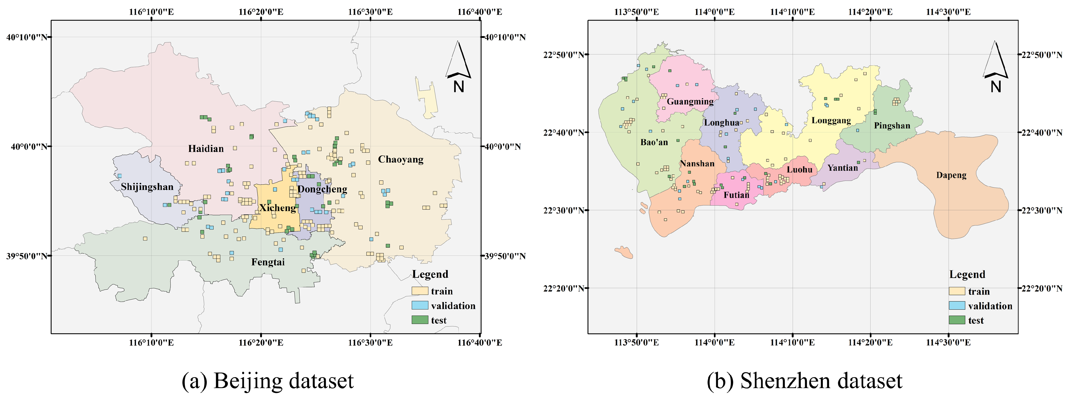
We created two new land use segmentation datasets with two categories: park and non-park. Parks that are too large or too small are excluded, because topological relationships among land cover objects in a park area cannot be well expressed by fixed-size image blocks at the current resolution. For a large park, an image block cannot reflect the overall spatial structure of it. For a small park, land cover data are not sufficiently refined to support the segmentation of tiny regions. In the Beijing dataset, we selected 157 parks of appropriate size in Beijing, China. In the Shenzhen dataset, we selected 99 parks in Shenzhen, Guangdong province, China. Due to the different shapes of these parks, we cropped them into image blocks of size 256 × 256 to facilitate the subsequent process. These samples are then randomly split into training, validation, and test sets in a 4:1:1 ratio using parks as units, which prevents data leakage. Samples in these sets are evenly distributed across districts (see Figure 3). Each sample has three components obtained in 2015: a VFSR image, a park label, and a land cover label.
The VFSR images with RGB bands come from Google Earth imagery. These images are at a zoom level of 16, with a resolution of 1.8 m for the Beijing dataset and 2.2 m for the Shenzhen dataset. They are cloud free after careful selection, and most of them were taken between July and September of 2015. To expand the dataset, we realized dataset augmentation through adaptively sliding windows with the premise of preserving the park’s integrity as much as possible. The augmented training dataset is abbreviated as “training-aug”. The distribution of samples in these two datasets can be seen in Table 1 and Table 2.
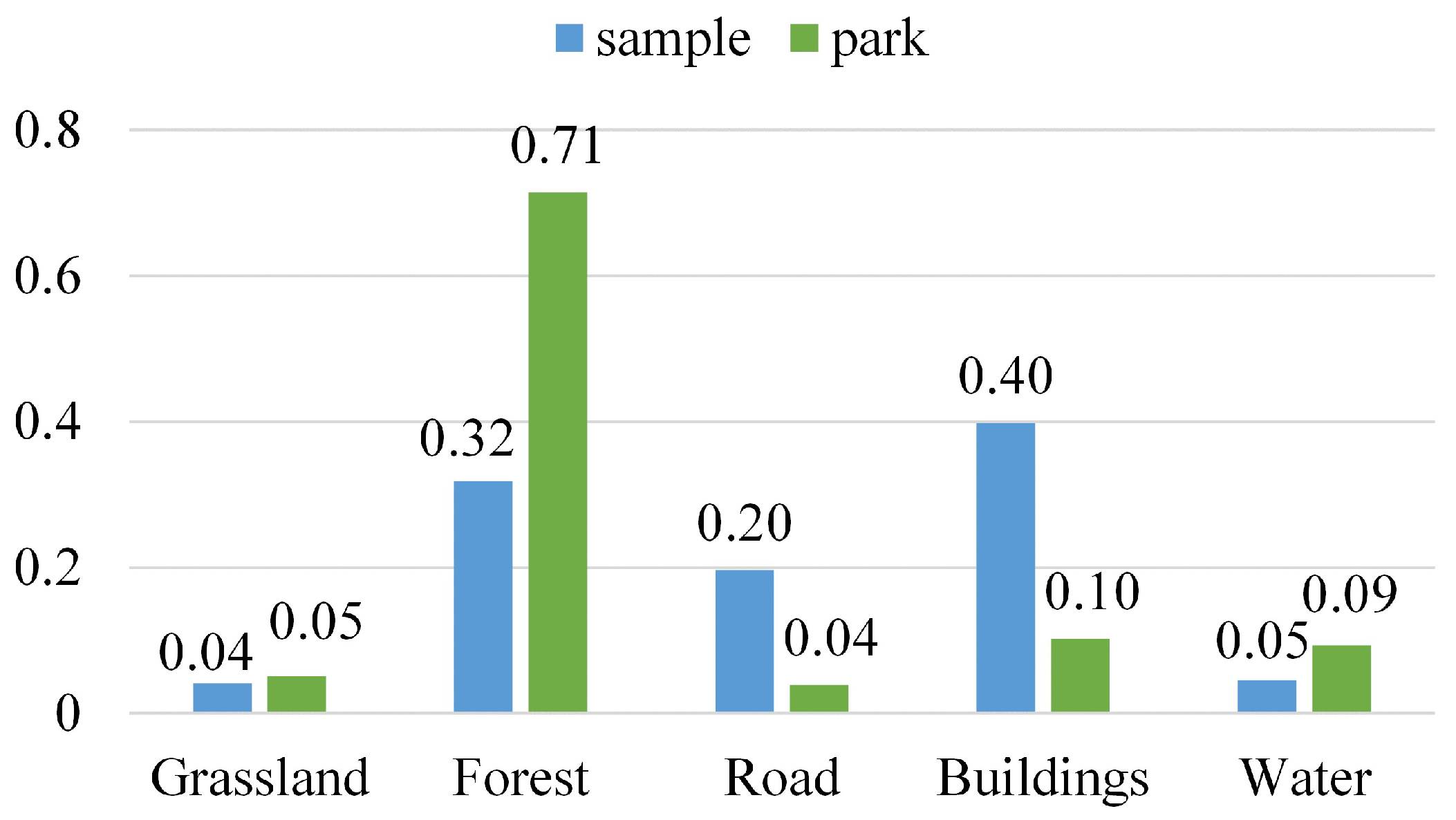
Park labels are made by manual correction on the basis of the OpenStreetMap (OSM) project and area of interest (AOI) data collected from Baidu Map. After reprojection and rasterization, the corrected park vector data are then transformed into raster labels. The land cover product, with a spatial resolution of 2 m, is generated from GF-1 data and contains 13 categories. By visual interpretation, we label unknown regions with the other 12 categories. Afterwards, these 12 categories (except the unknown class) are merged into five classes: grass, forest, buildings, road, and water. The class distribution of the processed land cover data is shown in Figure 4. Blue bars indicate the distribution of samples in all areas, while green bars denote the distribution of park regions. It is worth noting that land cover labels are reprojected and resampled as the coordinate system and resolution of this product do not match images.

3.2. Hyperparameters Configuration

CHeGCN has four components: the CNN module, the heterogeneous graphs construction, the GCN module, and the classifier. The output dimensions of the CNN module are 32. The segment number n and compactness c of SLIC are set to 50 and 10, respectively. Parameter n is the approximate number of segments, and c balances the color proximity and space proximity. There are 3 layers each with 32 units in the GCN module. Each GCN layer is followed by a batch normalization [49] layer and a ReLU activation layer. The fused feature maps are followed by a 1 × 1 convolutional layer, a softmax function, and the cross-entropy loss. We use the Adam optimizer [50] to train CHeGCN for 130 epochs, with four examples per mini-batch. All hyperparameters are determined by the performance in the validation dataset, and the same hyperparameter configuration is used for both qualitative and quantitative results. Our code (Code is available at: https://github.com/Liuzhizhiooo/CHeGCN-CNN_enhanced_Heterogeneous_Graph) is implemented with Python-3.6 and PyTorch-1.10.2 and is accessed on 6 October 2022.
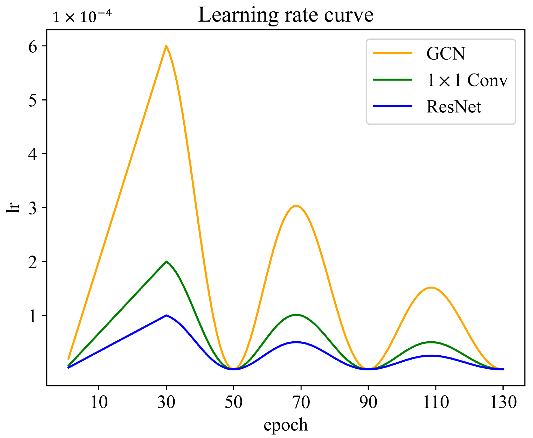
The learning rate (lr) parameters of modules should be different because the architectures of the CNN module and the GCN module are different. Meanwhile, the ResNet backbone is pretrained, thus the lr of it is set lower than convolutional layers that are used in dimension deduction and the classifier. Specifically, the maximum lr of the GCN module, the ResNet-18 backbone, and the 1 × 1 convolutional layers are 6 × 10 4 , 1 × 10 4 , and 2 × 10 4 , respectively. Furthermore, we adopt the warm-up strategy [41], the cosine annealing warm restarts schedule [51], and periodically decay the amplitude. The lr curves are shown in Figure 5, and the lr schedule is formulated as Equation (5):
l r t = 1 2 β t l r m a x ( 1 + cos ( t π ) )
where:
  • l r t is the learning rate at current epoch t;
  • β is the periodic decay factor and is set to 1 / 2 ;
  • l r m a x is the maximum learning rate of modules,
  • t is a temporary variable and t = t T 0 T ;
  • T 0 is the number of epochs for warm-up and is set to 30;
  • T is the number of epochs between two warm restarts and is set to 20.
Figure 5. Learning rate schedule, which combines the warm-up strategy, cosine annealing warm restarts schedule, and periodic decay. The maximum learning rates of different components in CHeGCN are different.
Remotesensing 14 05027 g005
Moreover, the training details of these state-of-the-art models for comparison are as follows. The pretrained ResNet-18, with the last two down-sampling layers removed, serves as the backbone for FCN, PSPNet, DeepLabv3, and GloRe. All compared models adopt the learning rate schedule in Equation (5) with l r m a x = 1 × 10 4 . We employ a heuristic strategy rather than grid search to determine the model structure and the hyperparameters because there are a lot of parameters in our model. Specifically, we first determine the model’s configuration, then the learning rate hyperparameters, and finally other parameters such as batch size and segmentation scale. All of these parameters are determined by the performance in the validation dataset. For some key parameters, such as model depth and segmentation scale, we conducted detailed experiments in the discussion section. It is worth noting that all quantitative metrics are obtained by the model with the maximum OA index on the validation dataset.

3.3. Comparison of Classification Performance

Table 3 and 
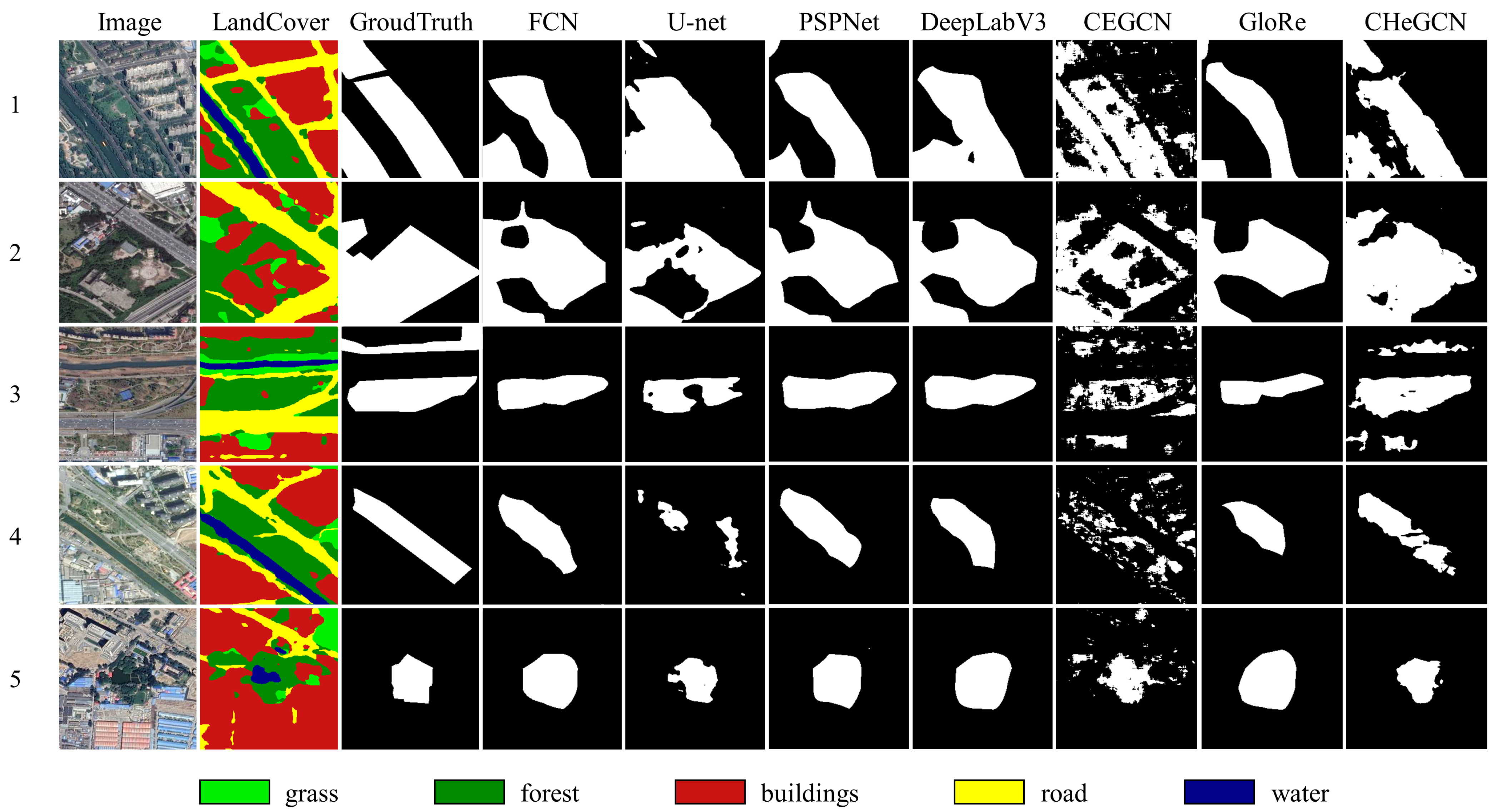
Table 4 exhibit the segmentation scores (%) of CHeGCN and six state-of-the-art models in terms of OA, Kappa, and IoU in two datasets. Meanwhile, we show the qualitative segmentation results of all methods in Figure 6.
In the Beijing dataset, our model performs the best and outperforms the second one by nearly 3.5% on the IoU metric. All CNNs achieve a similar performance, except U-net. Under the condition of limited samples, U-net behaves worse than other CNNs because it is trained from scratch. Meanwhile, we observe that the performance of the graph-based model CEGCN is unsatisfactory. This could be due to insufficient local spatial feature extraction. CEGCN is developed for hyperspectral images with abundant spectral information, which extracts pixel-level features. GloRe has a marginal improvement over CNNs, which benefits from the constructed long-distance relationships. However, GloRe builds graphs by applying convolutions to images, resulting in mismatches between nodes in interaction space and land cover units. Therefore, the improvement is not significant. Compared to GloRe, CHeGCN builds graphs based on land cover elements and achieves better performance.
Similarly to the previous dataset, the Shenzhen dataset demonstrates CHeGCN’s advantages over other models. CHeGCN outperforms CNNs (e.g., DeepLabv3) and homogeneous GCNs (e.g., GloRe) by approximately 5% on the Kappa and IoU indices. GloRe, on the other hand, performs worse than PSPNet and U-net, demonstrating its instability. The topological relationships among land cover units cannot be properly established since GloRe builds graphs on virtual nodes. In contrast, CHeGCN achieves stable improvement over CNNs.
We further display the qualitative segmentation results of several test samples in Figure 6. CNNs and CEGCN tend to classify all forest and water pixels as parks (see sample 1), regardless of the topological positions of these pixels. Meanwhile, CNNs, CEGCN, and GloRe fail to treat park regions as a whole. They classify buildings in the marked area of sample 2 as non-park. CNNs ignore the narrow park area in sample 3 as pooling operations of deep CNN severely destroy the spatial structure. In contrast, CHeGCN removes the last four convolutional layers of ResNet-18 to extract shallow CNN features, which are beneficial for small object recognition. The same goes for samples 4 and 5, where the predictions of CNNs tend to be over-smoothed and blurred. The noisy results of CEGCN indicate its lack of spatial features. Comparatively, CHeGCN yields more accurate results.

3.4. Ablation Experiments

The improvement in the performance of CHeGCN model can be attributed to two factors: the heterogeneous graph-based reasoning and the pretrained CNN module. We designed the following experiments on the Beijing dataset to demonstrate the effectiveness of these factors. It is worth noting that hyperparameters in ablation experiments remain unchanged unless otherwise specified.
First, we conduct experiments to demonstrate the effectiveness of graph reasoning. We build a CNN model with the same structure as CHeGCN, except that the CNN model substitutes the GCN module with three convolutional layers. These layers have the same hidden units as the GCN layers. As a result, rows 3 and 5 in Table 5 show that the GCN module plays an important role, improving the accuracy by nearly 3.5%, 8.5%, and 8.5% in terms of OA, Kappa, and IoU, respectively.
Furthermore, considering the situation in which there are no land cover data available, CHeGCN cannot use meta-path parameters to refine edge weights and degenerates to the CNN-enhanced HOmogeneous Graph Convolutional Network (CHoGCN). The sole difference from CHeGCN is that nodes in CHoGCN do not have land cover labels. Therefore, CHoGCN calculates the edge weights by (1). Compared with CHeGCN, there is a performance drop (nearly 2.5% in Kappa and IoU) in CHoGCN. This suggests that heterogeneous graphs have a stronger inference capability than homogeneous graphs. Meanwhile, CHoGCN outperforms the CNN model, demonstrating the effectiveness of graph reasoning once again.
Moreover, CNN features boost the performance of graph-based models. We report the accuracy metrics of the HOmogeneous Graph Convolutional Network (HoGCN) and HEterogeneous Graph Convolutional Network (HeGCN), neither of which employs a CNN module. The differences between HeGCN and CHeGCN are the initialization of node features and feature fusion. Node features in HeGCN are the average spectral features in superpixels of the input image, whereas CHeGCN takes the mean value of the CNN module’s feature maps as node features. Moreover, HeGCN only employs the GCN output to classify without using CNN feature maps. The same goes for the differences between HoGCN and CHoGCN. The CNN module significantly improves the Kappa of HoGCN and HeGCN, as shown in Table 5. Meanwhile, HeGCN outperforms HoGCN, which is consistent with the previous conclusion that land cover data are beneficial.

3.5. Visualization Analysis

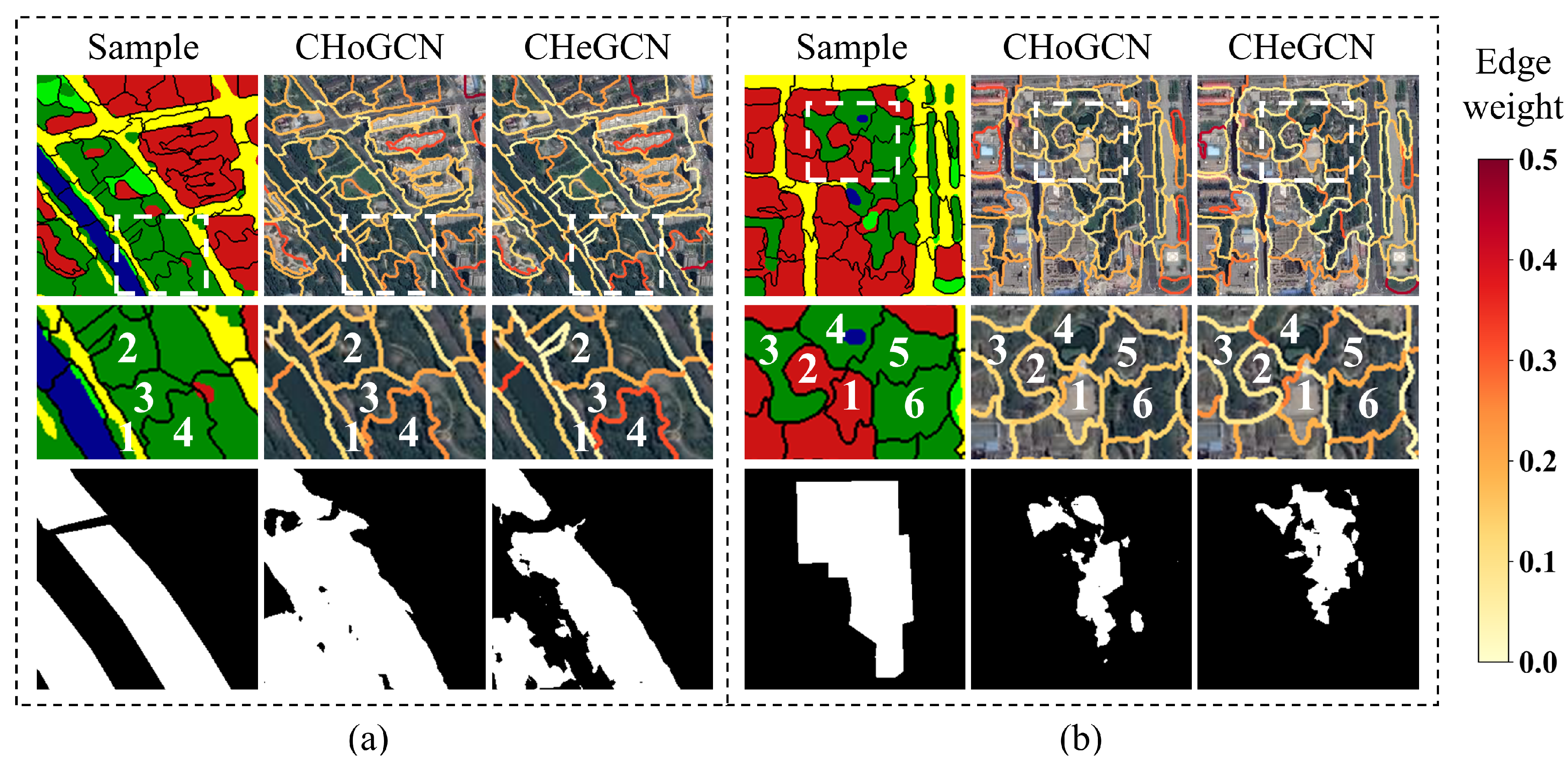
In this section, we analyze the underlying mechanism of CHeGCN. We visualize edge weights among adjacent land cover objects to observe topological relations among land cover objects in parks. CHoGCN is compared with the proposed CHeGCN to illustrate the advantages of heterogeneous graphs. Furthermore, we interpret segmentation results with meta-path parameters. We select two samples to show the edge weights and segmentation results of CHoGCN and CHeGCN in Figure 7. The top row contains land cover data overlaid with superpixel boundaries, and the edge weights of models. The second row includes the zoomed-in views of the highlight boxes in the first row. The third row consists of the ground truth label, and the predictions of models.
As shown in Figure 7a, CHoGCN misclassifies the road and water regions in the lower left of the image. Due to the improper selection of edge weights, the topological relationships are insufficiently constructed. As mentioned previously, roads generally form the boundaries of parks. This is consistent with land cover distribution statistics in Figure 4, where the number of road pixels in parks is much less than that in all regions. However, the edge weight of CHoGCN between a road object and a forest object is high. Specifically, the edges between a road node (1) and forest nodes (2, 3, 4) in CHoGCN are high, which are orange-colored. This will reduce the interclass variance in the feature aggregation, leading to the false positive classification. CHeGCN decreases the edge weights (rendered in yellow) between road and forest objects, making these nodes further apart in the feature space.
Figure 7b shows another example. Because of inadequate use of neighboring information, CHoGCN incorrectly labels the building area in the park as non-park. CHeGCN reduces intraclass variance during feature aggregation to smooth local variations, which finally achieves global perception. In detail, the forest superpixels (nodes 3, 4, 5, 6) surrounding the building are more closely connected than those of CHoGCN, and the corresponding edges in CHeGCN tend to be red. As a result, the features of the building regions (nodes 1, 2) tend to be similar to those of their neighbors, making them easier to recognize as parks.
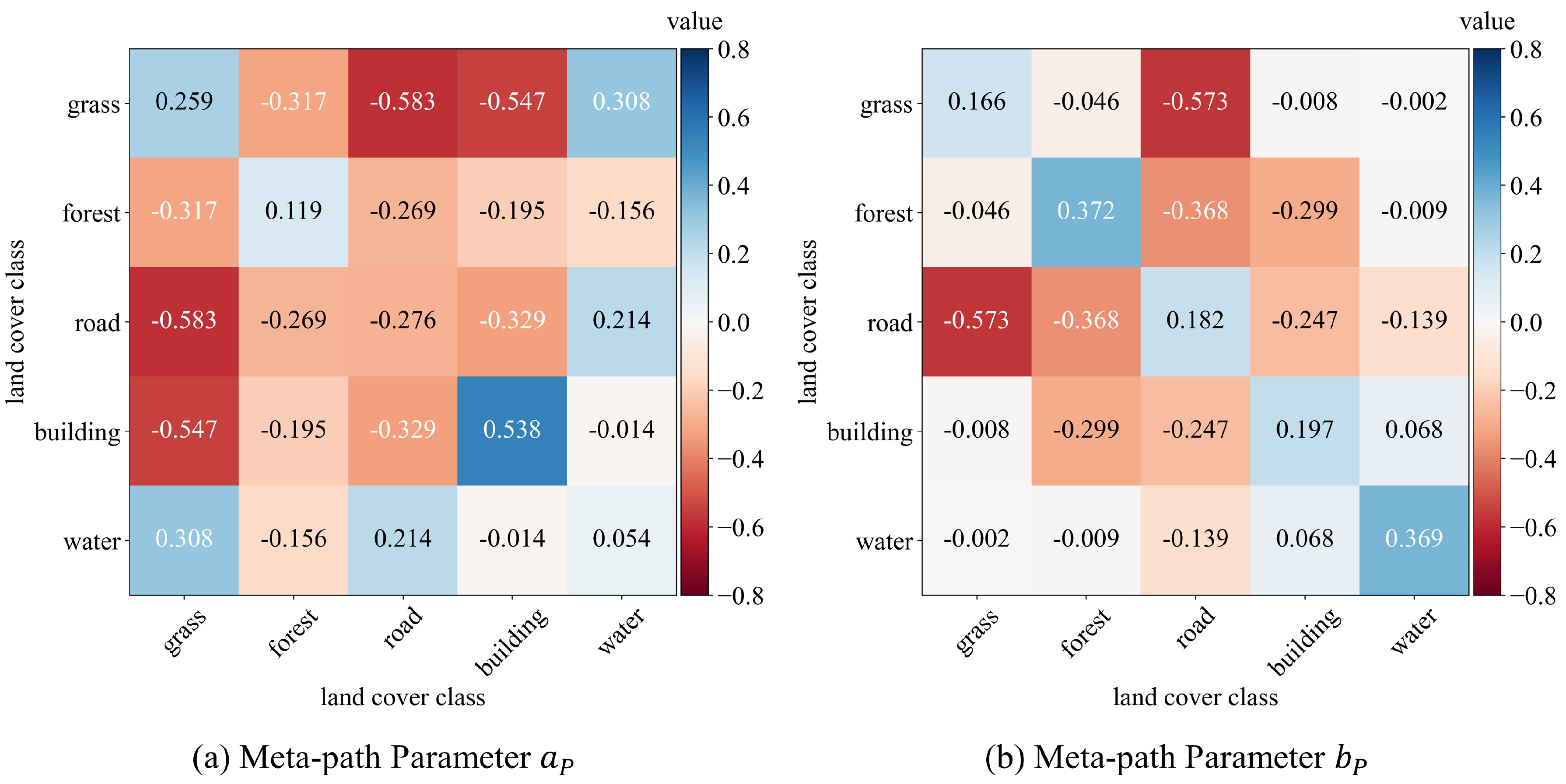
We visualize meta-path parameters a P , b P in Figure 8 because they play a critical role in heterogeneous graph construction (the calculation equation is seen in Equation (2)). Combined with the above cases, we find these parameters interpretable. Almost all parameters of the self-connection meta-path are positive, which is profitable for decreasing the intraclass variance. Most of the values related to roads are negative, especially the parameters of meta-path “road-grass” and “road-forest”. As such, meta-path parameters are advantageous for the segmentation of the scene in Figure 7a. Meanwhile, despite being negative, the absolute values of the parameters of the meta-path “buildings-forest” are relatively small. These behaviors make it possible to realize global recognition for segmentation, such as the case in Figure 7b. From the above analysis, we find that meta-path-based adjacency matrix calculation in Equation (2) greatly enhances graph reasoning capability.
To summarize, the mechanism of the heterogeneous graph-based model is to adaptively adjust interclass and intraclass variance based on topological relations. We take the sample in Figure 7a to show the difference in feature distribution before and after the GCN module, where the feature dimension is reduced to two by principal component analysis (PCA) [52]. As shown in Figure 9a, the CNN features of water nodes are close to those of park nodes since the water regions are located in the middle of two parks. After the GCN module, the interclass variance between the forest and water nodes are increased (see Figure 9b), which is consistent with the analysis of the edge weights in Figure 7a. Moreover, the intraclass variance of buildings is increased after the node feature aggregation. This makes it possible to distinguish building nodes inside parks from those outside parks. The building nodes outside parks are gathered together and move away from the park cluster because the a P of the meta-path “buildings-buildings” is high. Finally, park nodes form a pure cluster.

4. Discussion

In this section, we further investigated some critical hyperparameters on the Beijing dataset. Meanwhile, we analyze the reasons behind these phenomena in combination with previous findings.

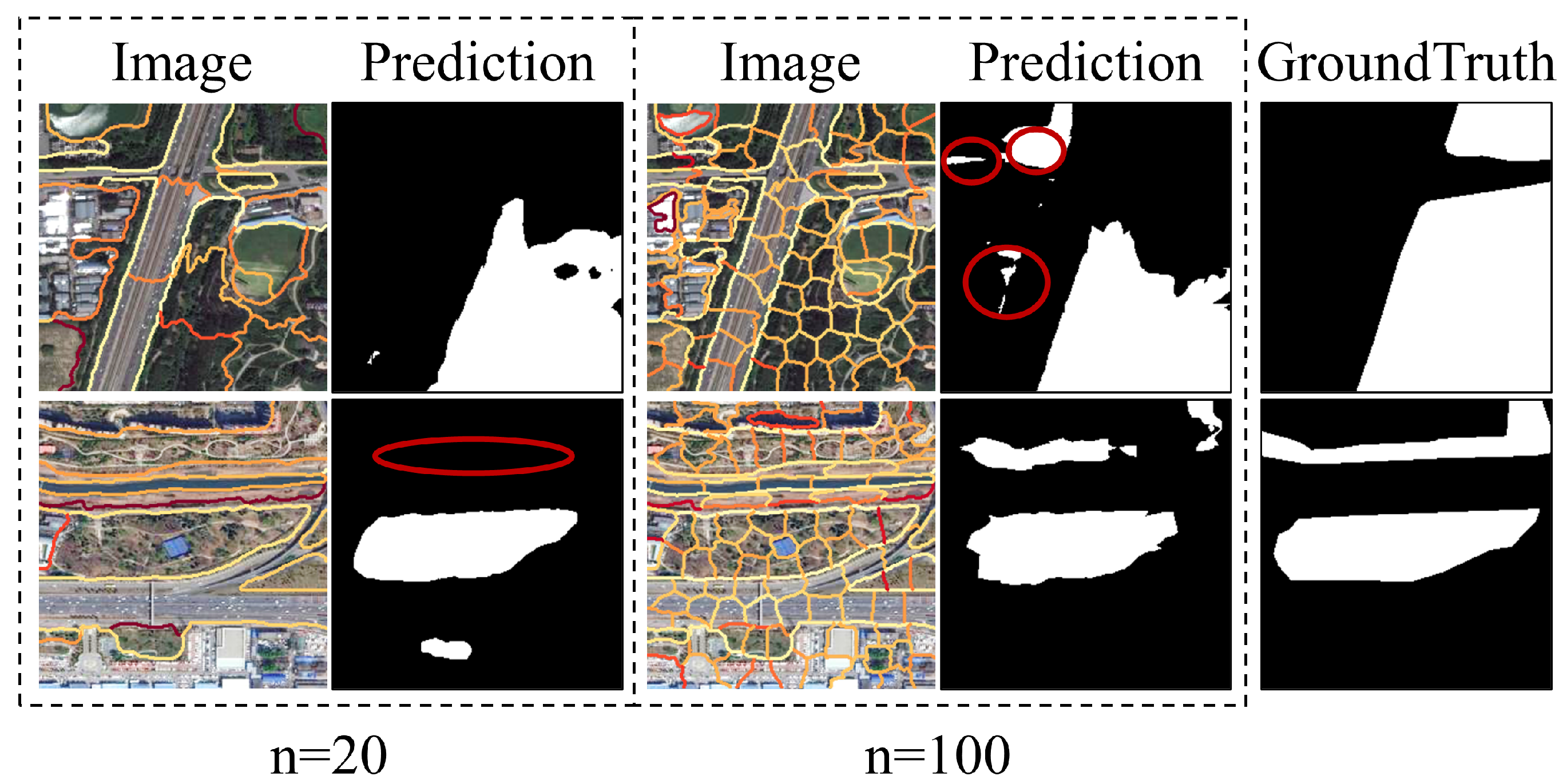
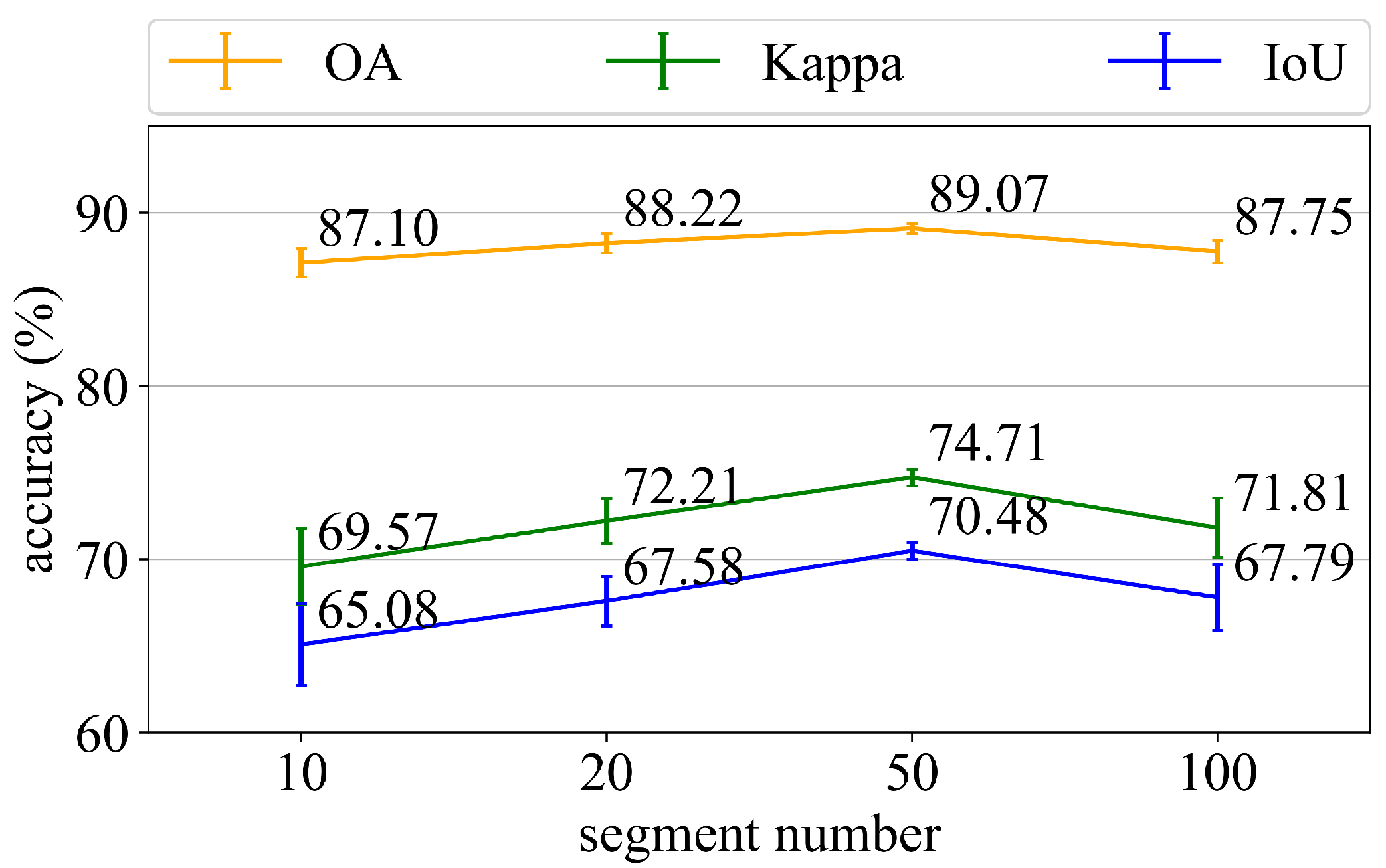
4.1. Influence of Segmentation Scale

Graph size is determined by the segmentation scale. The larger n is, the more nodes there are in the graph. Large objects are easily over-smoothed, whereas small objects are noisy. Figure 10 shows that, on the first sample, the model performs better with a smaller n = 20, which filters out the noisy regions. When n = 100, however, the long and narrow park can be better identified.
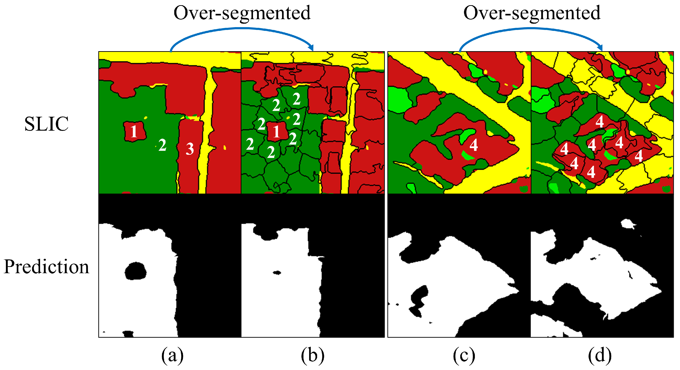
Generally, we prefer appropriate over-segmentation, which ensures that the segmented regions are homogeneous and preserves more spatial details. Furthermore, we believe that proper over-segmentation can better establish topological relationships. When relations are described by large objects in Figure 11a, the “surrounded” relation is the same as the “adjacent” relation because there is only a single edge between node 2 and node 1, and the same thing between node 2 and node 3. By contrast, there are more edges between node 1 and its surrounding nodes in Figure 11b if over-segmented. Thus, node 1 is more likely to be identified as a park node. However, when there is a large building in a park, such as node 4 in Figure 11c, the prediction result will be unsatisfactory if over-segmented. As aforementioned, CHeGCN can reduce intraclass variation, causing node 4 in Figure 11d to move away from the park cluster after over-segmentation. As a result, the accuracy of CHeGCN rises at first, and then falls as n increases in Figure 12. Meanwhile, the standard deviation is high when n is too high or too low, indicating that using an appropriate segmentation scale can produce more stable results. The determination of the segment number is data-dependent and heuristic.

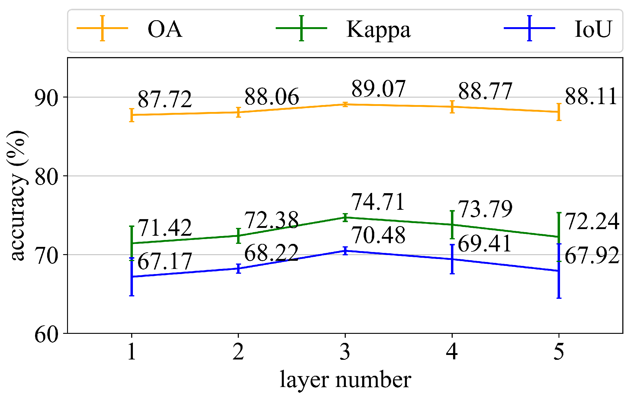
4.2. Influence of Network Depth

Although GCNs have shown promise, their architectures are much shallower than those of CNNs. Because of the vanishing gradient problem, most current GCNs generally contain 2–4 layers. The variation of model depth will greatly influence the performance of the model as the layer number is limited. We investigate the impact of CHeGCN depth in the following experiments. In more detail, we evaluate the performance of CHeGCN with 1–5 layers, where the number of hidden units in each layer is 32. Other hyperparameters are unchanged from previously.
As seen in Figure 13, the best choice of model depth is three. Excessively shallow or excessively deep networks have larger deviation values. The model with fewer layers captures an insufficient global context, resulting in a large variation in the extracted features. The model with more layers, on the other hand, is prone to over-smoothing, which ultimately makes nodes of different types indistinguishable in the feature space. 
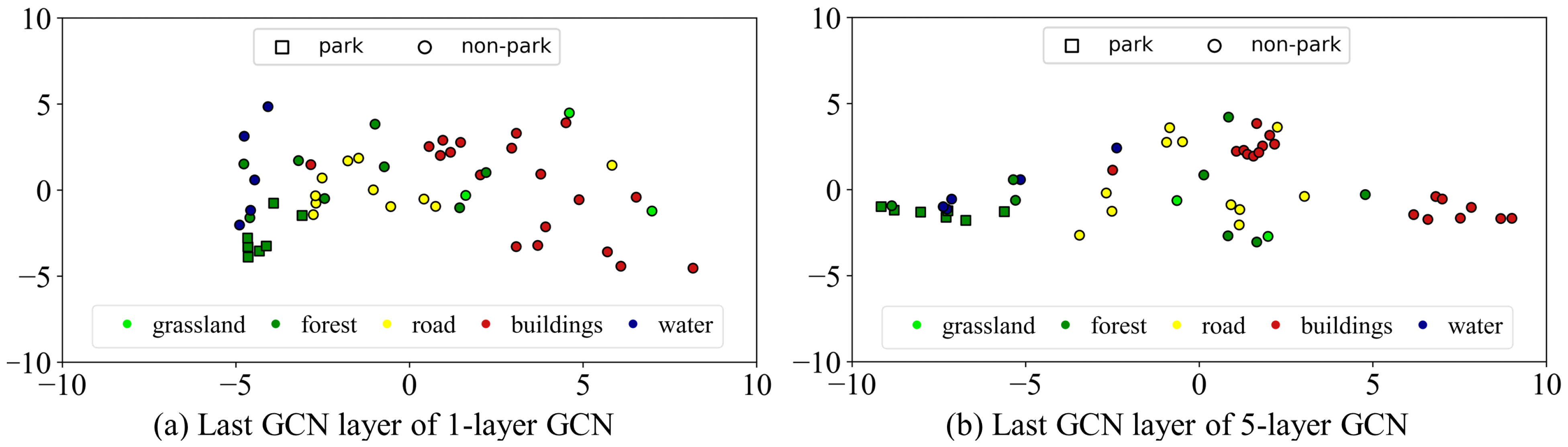
Figure 14 depicts the feature distributions of the last GCN layer in the single-layer CHeGCN and the five-layer CHeGCN. The intraclass variance of the shallow GCN is high, where the building nodes are discretely distributed. Meanwhile, the interclass variance of the deeper GCN is minor. The water and forest nodes are mixed together, and it is difficult to distinguish. As a result, building an extremely shallow or deep GCN is not recommended. In all of the other experiments, the layer number is fixed to three.

4.3. Spatially Adjacent vs. Global Adjacent

As mentioned above, land use segmentation requires global context information. CHeGCN stacks k GCN layers to aggregate features from k-hop neighborhoods based on topological relations. Another solution is to connect a pixel to all pixels [43,53]. Inspired by it, we propose a non-local CHoGCN and a non-local CHeGCN, which calculate the response at a given superpixel as a weighted sum of all superpixels. We compare the results between non-local models and the local connected models. Each experiment is repeated five times, with the average of the indices (OA, Kappa, and IoU) recorded in Table 6.
We observe that both non-local CHoGCN and non-local CHeGCN models perform worse than CHoGCN and CHeGCN, respectively, as model depth is three. Considering that fully connected non-local models are prone to overfitting, we compare these models in a single-layer structure. However, these single-layer non-local networks still fail to compete with the single-layer local connected models. On the one hand, it is difficult to train a fully connected network with limited samples. On the other hand, park segmentation relies heavily on topological relations, where non-local models fail to extract dependencies among heterogeneous regions and cannot capture local spatial structures. Furthermore, we discover that a non-local structure has far more negative effects on CHeGCN than on CHoGCN. When adopting the non-local strategy, IoU drops (ΔIoU) by 4.55% and 6.89% for 3-layer CHoGCN and 3-layer CHeGCN, respectively. This demonstrates that the performance of heterogeneous graph-based models will suffer greatly when meta-path parameters are not appropriately selected.

4.4. Other Types of Land Use

Based on the aforementioned experiments and analysis, we demonstrated the great improvements in park segmentation with land cover data. Furthermore, we believe that, in addition to parks, there are other types of land use that can benefit from the land cover information. Some land use categories are combinations of multiple land cover components, and different land use categories have distinct combination patterns. For example, wetlands typically consist of water and grass regions while urban parks may also contain buildings. In addition, the location of land use units is closely tied to the land cover distribution. For instance, commercial areas regularly emerge in the center of building areas, and fields are rarely seen among buildings. However, several land use categories, such as forest, grass, and water, may obtain slight improvements given that they share similar definitions with land cover.

4.5. Imagery with Multiple Spectral Bands

In this article, the images in our datasets only contain RGB bands, while most of VFSR images contain four spectral bands (RGB + near-infrared). The simple method to generalize our model to VFSR images with four bands is to take the RGB bands. On the one hand, the primary information for land use segmentation is included in RGB bands. On the other hand, as the short-wave infrared spectrum predominantly provides relevant information for vegetation recognition, the additional land cover information provides supplemental information for vegetation. In addition, we could modify the CNN module to better exploit the multi-spectral data. For example, we can substitute the ResNet-18 backbone with U-net, which does not restrict the band number at 3. Meanwhile, the U-net trained from scratch may require more data to obtain comparable results.

5. Conclusions

In this paper, we propose a heterogeneous graph-based model, CHeGCN, to infer land use from land cover. Unlike prior work that builds graphs solely on images, we introduce land cover data to better estimate the topological relations among geo-objects. With the assistance of land cover information, CHeGCN achieves approximately 2.5% IoU improvements over CHoGCN in two datasets. The mechanism behind this is that the ability of graph reasoning is enhanced by adaptively adjusting the edge weights of labeled nodes. In addition, our CHeGCN produces more accurate segmentation results. CHeGCN performs nearly 3.5% and 5% better than current methods, namely CNNs and GCNs, respectively. Meanwhile, we comprehensively analyze the underlying mechanisms. In conclusion, CHeGCN is capable of processing heterogeneous data, which greatly improves land use segmentation results. Inspired by the image pyramid, we believe the multi-scale architecture of graphs will be beneficial for building topological relationships. In future work, the multi-scale structure will be explored to better exploit pretrained deep CNN features and GCN features at different segmentation scales.

Author Contributions

Conceptualization, Z.-Q.L. and Z.Z.; methodology, Z.-Q.L. and P.T.; software, Z.-Q.L. and W.Z.; data curation, Z.-Q.L.; writing—original draft, Z.-Q.L.; writing—review and editing, Z.-Q.L. and Z.Z.; visualization, Z.-Q.L.; supervision, Z.Z. All authors have read and agreed to the published version of the manuscript.

Funding

This research was funded by the National Key R&D Program of China (Grant No. 2021YFB3900503), the Youth Innovation Promotion Association, CAS (No. 2022127), and “Future Star” Talent Plan of Aerospace Information Research Institute, Chinese Academy of Sciences (No. 2020KTYWLZX03 and No. 2021KTYWLZX07).

Acknowledgments

We gratefully acknowledge the free access to land cover data (https://data.casearth.cn/sdo/detail/60e55fca819aec59a2af708d and https://data.casearth.cn/sdo/detail/60e55fca819aec59a2af708f, accessed on 7 July 2021) provided by the Big Earth Data Science Engineering Project (CASEarth) launched by the Chinese Academy of Sciences (CAS) and the International Research Center of Big Data for Sustainable Development Goals (CBAS).

Conflicts of Interest

The authors declare no conflict of interest.

References

  1. Patino, J.E.; Duque, J.C. A review of regional science applications of satellite remote sensing in urban settings. Comput. Environ. Urban Syst. 2013, 37, 1–17. [Google Scholar] [CrossRef]
  2. Vitousek, P.M.; Mooney, H.A.; Lubchenco, J.; Melillo, J.M. Human domination of Earth’s ecosystems. Science 1997, 277, 494–499. [Google Scholar] [CrossRef] [Green Version]
  3. Zhu, Z.; Zhou, Y.; Seto, K.C.; Stokes, E.C.; Deng, C.; Pickett, S.T.; Taubenböck, H. Understanding an urbanizing planet: Strategic directions for remote sensing. Remote Sens. Environ. 2019, 228, 164–182. [Google Scholar] [CrossRef]
  4. Comber, A.J.; Brunsdon, C.F.; Farmer, C.J. Community detection in spatial networks: Inferring land use from a planar graph of land cover objects. Int. J. Appl. Earth Obs. Geoinf. 2012, 18, 274–282. [Google Scholar] [CrossRef] [Green Version]
  5. Li, M.; Stein, A. Mapping land use from high resolution satellite images by exploiting the spatial arrangement of land cover objects. Remote Sens. 2020, 12, 4158. [Google Scholar] [CrossRef]
  6. Zhang, C.; Sargent, I.; Pan, X.; Li, H.; Gardiner, A.; Hare, J.; Atkinson, P.M. An object-based convolutional neural network (OCNN) for urban land use classification. Remote Sens. Environ. 2018, 216, 57–70. [Google Scholar] [CrossRef] [Green Version]
  7. Cihlar, J.; Jansen, L.J. From land cover to land use: A methodology for efficient land use mapping over large areas. Prof. Geogr. 2001, 53, 275–289. [Google Scholar] [CrossRef]
  8. Walde, I.; Hese, S.; Berger, C.; Schmullius, C. From land cover-graphs to urban structure types. Int. J. Geogr. Inf. Sci. 2014, 28, 584–609. [Google Scholar] [CrossRef]
  9. Barnsley, M.J.; Barr, S.L. Distinguishing urban land-use categories in fine spatial resolution land-cover data using a graph-based, structural pattern recognition system. Comput. Environ. Urban Syst. 1997, 21, 209–225. [Google Scholar] [CrossRef]
  10. Zhang, W.; Tang, P.; Corpetti, T.; Zhao, L. WTS: A Weakly towards strongly supervised learning framework for remote sensing land cover classification using segmentation models. Remote Sens. 2021, 13, 394. [Google Scholar] [CrossRef]
  11. Chen, J.; Chen, J. GlobeLand30: Operational global land cover mapping and big-data analysis. Sci. China Earth Sci. 2018, 61, 1533–1534. [Google Scholar] [CrossRef]
  12. Gong, P.; Wang, J.; Yu, L.; Zhao, Y.; Zhao, Y.; Liang, L.; Niu, Z.; Huang, X.; Fu, H.; Liu, S.; et al. Finer resolution observation and monitoring of global land cover: First mapping results with Landsat TM and ETM+ data. Int. J. Remote Sens. 2013, 34, 2607–2654. [Google Scholar] [CrossRef] [Green Version]
  13. Yu, F.; Koltun, V. Multi-scale context aggregation by dilated convolutions. arXiv 2015, arXiv:1511.07122. [Google Scholar]
  14. Liu, W.; Rabinovich, A.; Berg, A.C. Parsenet: Looking wider to see better. arXiv 2015, arXiv:1506.04579. [Google Scholar]
  15. Zhao, H.; Shi, J.; Qi, X.; Wang, X.; Jia, J. Pyramid scene parsing network. In Proceedings of the IEEE Conference on Computer Vision and Pattern Recognition, Honolulu, HI, USA, 21–26 July 2017; pp. 2881–2890. [Google Scholar]
  16. Li, H.; Xiong, P.; An, J.; Wang, L. Pyramid attention network for semantic segmentation. arXiv 2018, arXiv:1805.10180. [Google Scholar]
  17. Chen, L.C.; Papandreou, G.; Kokkinos, I.; Murphy, K.; Yuille, A.L. Semantic image segmentation with deep convolutional nets and fully connected crfs. arXiv 2014, arXiv:1412.7062. [Google Scholar]
  18. Chen, L.C.; Papandreou, G.; Kokkinos, I.; Murphy, K.; Yuille, A.L. Deeplab: Semantic image segmentation with deep convolutional nets, atrous convolution, and fully connected crfs. IEEE Trans. Pattern Anal. Mach. Intell. 2017, 40, 834–848. [Google Scholar] [CrossRef] [Green Version]
  19. Chen, L.C.; Papandreou, G.; Schroff, F.; Adam, H. Rethinking atrous convolution for semantic image segmentation. arXiv 2017, arXiv:1706.05587. [Google Scholar]
  20. Chen, L.C.; Zhu, Y.; Papandreou, G.; Schroff, F.; Adam, H. Encoder-decoder with atrous separable convolution for semantic image segmentation. In Proceedings of the European Conference on Computer Vision (ECCV), Munich, Germany, 8–14 September 2018; pp. 801–818. [Google Scholar]
  21. Long, J.; Shelhamer, E.; Darrell, T. Fully convolutional networks for semantic segmentation. In Proceedings of the IEEE Conference on Computer Vision and Pattern Recognition, Boston, MA, USA, 7–12 June 2015; pp. 3431–3440. [Google Scholar]
  22. Ronneberger, O.; Fischer, P.; Brox, T. U-net: Convolutional networks for biomedical image segmentation. In Proceedings of the International Conference on Medical Image Computing and Computer-Assisted Intervention, Munich, Germany, 5–9 October 2015; Springer: Berlin/Heidelberg, Germany, 2015; pp. 234–241. [Google Scholar]
  23. Li, Y.; Gupta, A. Beyond grids: Learning graph representations for visual recognition. Adv. Neural Inf. Process. Syst. 2018, 31, 9225–9235. [Google Scholar]
  24. Chen, Y.; Rohrbach, M.; Yan, Z.; Shuicheng, Y.; Feng, J.; Kalantidis, Y. Graph-based global reasoning networks. In Proceedings of the IEEE/CVF Conference on Computer Vision and Pattern Recognition, Long Beach, CA, USA, 16–20 June 2019; pp. 433–442. [Google Scholar]
  25. Lucas, R.; Rowlands, A.; Brown, A.; Keyworth, S.; Bunting, P. Rule-based classification of multi-temporal satellite imagery for habitat and agricultural land cover mapping. ISPRS J. Photogramm. Remote Sens. 2007, 62, 165–185. [Google Scholar] [CrossRef]
  26. Hamilton, W.L. Graph representation learning. Synth. Lect. Artifical Intell. Mach. Learn. 2020, 14, 1–159. [Google Scholar]
  27. Hamilton, W.; Ying, Z.; Leskovec, J. Inductive representation learning on large graphs. Adv. Neural Inf. Process. Syst. 2017, 30, 1025–1035. [Google Scholar]
  28. Fout, A.; Byrd, J.; Shariat, B.; Ben-Hur, A. Protein interface prediction using graph convolutional networks. Adv. Neural Inf. Process. Syst. 2017, 30, 6533–6542. [Google Scholar]
  29. Rhee, S.; Seo, S.; Kim, S. Hybrid approach of relation network and localized graph convolutional filtering for breast cancer subtype classification. arXiv 2017, arXiv:1711.05859. [Google Scholar]
  30. Malisiewicz, T.; Efros, A. Beyond categories: The visual memex model for reasoning about object relationships. Adv. Neural Inf. Process. Syst. 2009, 22, 1222–1230. [Google Scholar]
  31. Kipf, T.N.; Welling, M. Semi-supervised classification with graph convolutional networks. arXiv 2016, arXiv:1609.02907. [Google Scholar]
  32. Liu, Q.; Xiao, L.; Yang, J.; Wei, Z. CNN-enhanced graph convolutional network with pixel-and superpixel-level feature fusion for hyperspectral image classification. IEEE Trans. Geosci. Remote Sens. 2020, 59, 8657–8671. [Google Scholar] [CrossRef]
  33. Wan, S.; Gong, C.; Zhong, P.; Pan, S.; Li, G.; Yang, J. Hyperspectral image classification with context-aware dynamic graph convolutional network. IEEE Trans. Geosci. Remote Sens. 2020, 59, 597–612. [Google Scholar] [CrossRef]
  34. Wan, S.; Gong, C.; Zhong, P.; Du, B.; Zhang, L.; Yang, J. Multiscale dynamic graph convolutional network for hyperspectral image classification. IEEE Trans. Geosci. Remote Sens. 2019, 58, 3162–3177. [Google Scholar] [CrossRef] [Green Version]
  35. Hong, D.; Gao, L.; Yao, J.; Zhang, B.; Plaza, A.; Chanussot, J. Graph convolutional networks for hyperspectral image classification. IEEE Trans. Geosci. Remote Sens. 2020, 59, 5966–5978. [Google Scholar] [CrossRef]
  36. Cui, W.; Yao, M.; Hao, Y.; Wang, Z.; He, X.; Wu, W.; Li, J.; Zhao, H.; Xia, C.; Wang, J. Knowledge and Geo-Object Based Graph Convolutional Network for Remote Sensing Semantic Segmentation. Sensors 2021, 21, 3848. [Google Scholar] [CrossRef] [PubMed]
  37. Hu, H.; Ji, D.; Gan, W.; Bai, S.; Wu, W.; Yan, J. Class-wise dynamic graph convolution for semantic segmentation. In Proceedings of the European Conference on Computer Vision, Glasgow, UK, 23–28 August 2020; Springer: Berlin/Heidelberg, Germany, 2020; pp. 1–17. [Google Scholar]
  38. Wang, X.; Ji, H.; Shi, C.; Wang, B.; Ye, Y.; Cui, P.; Yu, P.S. Heterogeneous graph attention network. In Proceedings of the World Wide Web Conference, San Francisco, CA, USA, 13–17 May 2019; pp. 2022–2032. [Google Scholar]
  39. Ouyang, S.; Li, Y. Combining deep semantic segmentation network and graph convolutional neural network for semantic segmentation of remote sensing imagery. Remote Sens. 2020, 13, 119. [Google Scholar] [CrossRef]
  40. Marmanis, D.; Datcu, M.; Esch, T.; Stilla, U. Deep learning earth observation classification using ImageNet pretrained networks. IEEE Geosci. Remote Sens. Lett. 2015, 13, 105–109. [Google Scholar] [CrossRef] [Green Version]
  41. He, K.; Zhang, X.; Ren, S.; Sun, J. Deep residual learning for image recognition. In Proceedings of the IEEE Conference on Computer Vision and Pattern Recognition, Las Vegas, NV, USA, 26 June–1 July 2016; pp. 770–778. [Google Scholar]
  42. Krizhevsky, A.; Sutskever, I.; Hinton, G.E. Imagenet classification with deep convolutional neural networks. Adv. Neural Inf. Process. Syst. 2012, 25, 84–90. [Google Scholar] [CrossRef] [Green Version]
  43. Mou, L.; Lu, X.; Li, X.; Zhu, X.X. Nonlocal graph convolutional networks for hyperspectral image classification. IEEE Trans. Geosci. Remote Sens. 2020, 58, 8246–8257. [Google Scholar] [CrossRef]
  44. Achanta, R.; Shaji, A.; Smith, K.; Lucchi, A.; Fua, P.; Süsstrunk, S. SLIC superpixels compared to state-of-the-art superpixel methods. IEEE Trans. Pattern Anal. Mach. Intell. 2012, 34, 2274–2282. [Google Scholar] [CrossRef] [PubMed] [Green Version]
  45. Velickovic, P.; Cucurull, G.; Casanova, A.; Romero, A.; Lio, P.; Bengio, Y. Graph attention networks. Stat 2017, 1050, 20. [Google Scholar]
  46. Bronstein, M.M.; Bruna, J.; LeCun, Y.; Szlam, A.; Vandergheynst, P. Geometric deep learning: Going beyond euclidean data. IEEE Signal Process. Mag. 2017, 34, 18–42. [Google Scholar] [CrossRef] [Green Version]
  47. Nair, V.; Hinton, G.E. Rectified linear units improve restricted boltzmann machines. In Proceedings of the ICML, Haifa, Israel, 21–24 June 2010; pp. 807–814. [Google Scholar]
  48. Camps-Valls, G.; Marsheva, T.V.B.; Zhou, D. Semi-supervised graph-based hyperspectral image classification. IEEE Trans. Geosci. Remote Sens. 2007, 45, 3044–3054. [Google Scholar] [CrossRef]
  49. Ioffe, S.; Szegedy, C. Batch normalization: Accelerating deep network training by reducing internal covariate shift. In Proceedings of the International Conference on Machine Learning, PMLR, Lille, France, 6–11 July 2015; pp. 448–456. [Google Scholar]
  50. Kingma, D.P.; Ba, J. Adam: A method for stochastic optimization. arXiv 2014, arXiv:1412.6980. [Google Scholar]
  51. Loshchilov, I.; Hutter, F. Sgdr: Stochastic gradient descent with warm restarts. arXiv 2016, arXiv:1608.03983. [Google Scholar]
  52. Tipping, M.E.; Bishop, C.M. Probabilistic principal component analysis. J. R. Stat. Soc. Ser. (Stat. Methodol.) 1999, 61, 611–622. [Google Scholar] [CrossRef] [Green Version]
  53. Wang, X.; Girshick, R.; Gupta, A.; He, K. Non-local neural networks. In Proceedings of the IEEE Conference on Computer Vision and Pattern Recognition, Salt Lake City, UT, USA, 18–22 June 2018; pp. 7794–7803. [Google Scholar]
Figure 1. Comparison of CNNs, homogeneous GCNs, and heterogeneous GCNs in feature extraction. The CNNs employ convolutions and pooling on regular regions to obtain feature maps and upsample them to the pixel level. Homogeneous GCNs first transform images into graphs by graph projection, and then apply GCN to obtain node-level features, and finally produce pixel-level feature maps by graph re-projection. Heterogeneous graphs differ from homogeneous graphs in the graph construction. Nodes of heterogeneous graphs are labeled with land cover classes in graph projection. Edge weights are determined by the corresponding node pair’s class. Graph projection is described in detail at the bottom, and graph reprojection is the inverse process of this.
Remotesensing 14 05027 g001
Figure 2. The architecture of CNN-enhanced HEterogeneous Graph Convolutional Network (CHeGCN) model. CHeGCN contains a CNN module and a GCN module, where the former focuses more on a local extraction pattern and the latter concentrates more on long-range dependency modeling. Before the GCN module is applied, the heterogeneous graph needs to be constructed. Nodes in the heterogeneous graph are determined by land cover superpixels and attributed by CNN feature maps. Edges are linked based on topological relations among nodes. Finally, GCN features are reprojected and fused with CNN features to accomplish park segmentation.
Remotesensing 14 05027 g002
Figure 3. Distribution of samples. These samples are divided into training, validation, and test sets in a ratio of 4:1:1. The data in each set are evenly distributed across districts.
Remotesensing 14 05027 g003
Figure 4. Land cover category distribution of all samples and park areas.
Remotesensing 14 05027 g004
Figure 6. Qualitative segmentation results of different methods. Five examples are provided for comparison of models. The first column is the images, the second one indicates the land cover data, the third one lists the corresponding ground truth, and the following columns exhibit the segmentation results of different models. The color table for land cover categories is listed at the bottom.
Remotesensing 14 05027 g006
Figure 7. Visualization of edge weights among land cover objects and the segmentation results. There are two examples shown in (a,b) and the numbers in the second row denote the index numbers of different nodes. The color bar on the right is used to render edge weights, with higher values making edges redder.
Remotesensing 14 05027 g007
Figure 8. Symmetric meta–path parameters a P , b P in edge calculation. The values are rendered with the color bar on the right, with positive values appearing in blue and negative values in red.
Remotesensing 14 05027 g008
Figure 9. Node feature distributions of the CNN module and the GCN module, where PCA reduces the feature dimension to two. The park cluster is highlighted with a blue dashed circle and nodes are rendered by their land cover categories.
Remotesensing 14 05027 g009
Figure 10. Comparison of qualitative results at different segmentation scales. Segmentation results of different segmentation scales are placed on the image. Predicted differences are marked with red circles.
Remotesensing 14 05027 g010
Figure 11. Two examples are provided to illustrate how the segmentation scale affects the construction of topological relations. In some cases, over-segmentation is beneficial for describing the topological relations of small objects. For instance, the “surrounding” relationship in (b) can be better expressed when the sample in (a) is over-segmented. However, describing the actual topological relations of large objects becomes more challenging when they are over-segmented. For example, (d) is the over-segmentation of (c). Since the topological relationship of node 4 is incorrectly expressed as being surrounded by buildings, the segmentation result of (d) is unsatisfactory.
Remotesensing 14 05027 g011
Figure 12. Quantitative comparison of CHeGCN at different segmentation scales.
Remotesensing 14 05027 g012
Figure 13. Quantitative comparison of models with different depths.
Remotesensing 14 05027 g013
Figure 14. The feature distributions of the last GCN layer in 1-layer CHeGCN and 5-layer CHeGCN.
Remotesensing 14 05027 g014
Table 1. The distribution of samples in Beijing dataset.
DatasetDongchengXichengHaidianChaoyangFengtaiShijingshanTotal
Training17143252227144
Training-aug53521661998527532
Validation449144237
Test549146240
Table 2. The distribution of samples in the Shenzhen dataset.
DatasetLuohuFutianNanshanYantianBao’anLonggangPingshanLonghuaGuangmingTotal
Training1312112231167792
Training-aug30403787346142422294
Validation13216314324
Test23416322124
Table 3. Quantitative comparison of different methods in the Beijing dataset.
ModelOAKappaIoU
FCN87.78 ± 0.6771.05 ± 1.9866.40 ± 2.22
U-net85.33 ± 0.6565.99 ± 2.0062.22 ± 2.18
PSPNet87.61 ± 0.3170.82 ± 0.9666.30 ± 1.12
DeepLabv387.86 ± 0.2071.46 ± 0.6566.97 ± 0.80
CEGCN79.67 ± 0.2651.67 ± 0.9149.42 ± 0.95
GloRe88.02 ± 0.6371.67 ± 1.9367.03 ± 2.26
CHeGCN89.07 ± 0.2974.71 ± 0.4970.48 ± 0.49
Table 4. Quantitative comparison of different methods in the Shenzhen dataset.
ModelOAKappaIoU
FCN87.46 ± 0.3965.17 ± 1.5757.85 ± 1.75
U-net87.51 ± 0.3966.07 ± 1.4259.10 ± 1.58
PSPNet87.66 ± 0.2166.37 ± 0.5359.33 ± 0.50
DeepLabv387.17 ± 0.2064.50 ± 0.9857.28 ± 1.18
CEGCN82.64 ± 0.2052.76 ± 1.0447.25 ± 1.09
GloRe87.33 ± 0.3364.83 ± 0.8957.52 ± 0.88
CHeGCN88.37 ± 0.4569.11 ± 1.7962.45 ± 2.11
Table 5. The quantitative comparison of different models in ablation experiments.
ModelOAKappaIoU
HoGCN78.60 ± 0.8350.04 ± 1.8048.77 ± 1.57
HeGCN83.12 ± 0.2761.86 ± 0.6759.25 ± 0.82
CNN85.63 ± 0.4066.10 ± 1.3561.85 ± 1.57
CHoGCN88.05 ± 0.6272.13 ± 1.3267.80 ± 1.20
CHeGCN89.07 ± 0.2974.71 ± 0.4970.48 ± 0.49
Table 6. Quantitative comparison of local and non-local CHeGCN.
LayerModelOAKappaIoUΔ IoU
1-layerCHoGCN87.4470.6966.39
Non-local CHoGCN86.9069.3064.97−1.42
CHeGCN87.7271.4267.17
Non-local CHeGCN86.8769.6765.69−1.48
3-layerCHoGCN88.0572.1367.80
Non-local CHoGCN86.0567.3963.25−4.55
CHeGCN89.0774.7170.48
Non-local CHeGCN86.3267.8763.59−6.89
Publisher’s Note: MDPI stays neutral with regard to jurisdictional claims in published maps and institutional affiliations.

