
Evaluation of Wind and Solar Insolation Influence on Ocean Near-Surface Temperature from In Situ Observations and the Geostationary Himawari-8 Satellite


1
Center for Space and Remote Sensing Research, National Central University, Taoyuan 320, Taiwan
2
Graduate Institute of Hydrological and Oceanic Sciences, National Central University, Taoyuan 320, Taiwan
Remote Sens. 2022, 14(19), 4975; https://doi.org/10.3390/rs14194975
Submission received: 15 September 2022
/
Revised: 30 September 2022
/
Accepted: 3 October 2022
/
Published: 6 October 2022
(This article belongs to the Special Issue Validation and Evaluation of Global Ocean Satellite Products)
Abstract
:The skin sea surface temperature (SST) observed by the geostationary Himawari-8 satellite and bulk SST, including four in situ observations from ships, drifters, Argo, and buoys constitute more than 90,000 SST pairs used to analyze near-surface temperature variations. From July 2015 to May 2022, an average SST bias of 0.10 °C and root mean square error of 0.99 °C were observed in the waters adjacent to Taiwan. This study effectively observed that the skin effect generated by ocean wind and solar shortwave radiation caused the occurrence of a cool skin layer and diurnal warm layer (DWL), and 90% of the SST bias was in a range of −1.55~1.71 °C. In the daytime, the skin layer received solar shortwave radiation, thus increasing temperature and causing a DWL. With the increase in insolation, the SST bias in the DWL became more obvious. During winter, strong wind, or low shortwave radiation, the DWL may disappear and turn into a cool skin layer. At night, the near-surface SST was dominated by the cool skin effect, but the DWL generated in the daytime would remain if the wind speed was weak. However, the different hydrological characteristics of the observation position and its distance from the coast could affect the results of the skin effect. Whether there is a rapid change in ocean stratification in a spatial grid of nearly four square kilometers needs to be explored in the future.
Keywords:
Himawari-8; skin SST; bulk SST; skin effect; diurnal warm layer; drifter; buoy; Argo; ship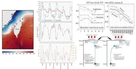
1. Introduction
The observation of sea surface temperature (SST) is necessary and important for the study of the global ocean heat budget and air-sea interaction. SST observed by satellite infrared radiometers is called skin SST, which characterized the temperature of the upper ~10 µm ocean layer, while SST observed at a certain depths in the near-surface, such as 1 m, 2 m or 5 m, is called bulk SST [1]. The main error sources of satellite measurements of SST are caused by dust, water vapor, clouds, the instrument, and skin effects [2]. In the case of low wind speed, the vertical and horizontal structures of skin and bulk SST vary greatly with time [3,4,5]. The SST bias between the skin and bulk SST is approximately 1 °C, but the bias may reach 3 °C due to different sampling depths [6]. The analysis and accurate calculation of the interaction between the skin effect and air-sea interaction is important [7], and wind can cause near-surface layer stratification [8]. At the global scale, the average cool skin effect observed by the ENVISAT satellite, drifting buoys and moorings is 0.13 °C [9]. In the waters near Australia, the average bias between skin SST and 7–9 m of bulk SST was 0.23 °C [10]. In the South China Sea, a range of 0–1 °C accounts for 95% of the SST bias, and the value most often appears in a range of 0.4–0.6 °C [11].
In addition to the cool skin layer, the bias between the skin and bulk SST could be affected by solar insolation to generate a diurnal warm layer (DWL) [5], and the formation of near-surface ocean stratification and DWL could change heat flux and transport [12], turbulence dissipation, lateral transport, shear instability, and mixing [13,14,15]. Using the bulk SST data from Argo, moorings, Seaglider, buoys, and satellite skin SST, significant DWL features have been observed all over the world ocean [16,17,18,19,20]. Using five long-term moorings, an average SST increase of 0.29 °C was observed in the open ocean, with a maximum of 3.38 °C and more than 221 days of SST increase exceeding 1 °C [17]. In the Indian Ocean, Seaglider found that the DWL appeared during solar radiation flux (>80 W/m2) and low wind speed (<6 m/s), and the temperature anomaly amplitude of the DWL was up to 0.8 °C with a daily average of 0.2 °C [18]. In the shallow waters of Australian coral reefs, buoy and satellite data observed that the average daily warming was approximately 0.4 °C at depths of 4–7 m and approximately 0.6–0.7 °C at shallow depths of 1–2 m. The maximum warming value was 2.1 °C. Diurnal heating depends on local features including water depth, location, and tide [19].
Since July 2015, the geostationary Himawari-8 satellite has provided high-resolution SST data every 10 min and every hour in the Pacific region. This not only improves the coverage of temperature at a temporal resolution but also provides a new understanding of high-frequency dynamic physical ocean processes with data at a 2 km spatial resolution, including surface upwelling [21,22,23], topographic eddies [24], island wakes [25], and pearl river plumes [26]. There are also more data samples that can be used to observe diurnal SST variations [27,28] and reconstruct SST using numerical methods [29]. Recent studies have observed that the maximum bias between skin SST and 8 m bulk SST in Australian waters can reach 2.23 °C [30]. It is very difficult to obtain skin and bulk SST at the same time and at the same location to explore the change in near-surface temperature, and a sufficient number of samples are needed to consider the feedback of solar insolation and ocean wind speed on SST. This study utilized the sea area adjacent to Taiwan as the research scope (Figure 1a); collected ship, drifter, and Argo data from the in situ SST quality monitor (iQuam); and used the 14 buoys (Figure 1b) to form more than 90,000 SST pairs of bulk and skin SST on cloud-free days, to analyze the characteristics of near-surface SST variations from July 2015 to May 2022. The observed samples cover the open ocean, nearshore and coastal areas, and the average SST ranged from 15 to 30 °C. This study examined (1) the bias between bulk and skin SST on long-term, monthly, and hourly scales; (2) whether the Himawari-8 SST could effectively observe skin effects for several hours to several days; (3) the influence of solar shortwave radiation on the skin SST, and (4) the influence of ocean surface wind intensity on near-surface SST.
2. Data
Four different types of bulk SST data obtained from two datasets were compared with the skin SST derived from the Himawari-8 satellite. The in situ SST quality monitor (iQuam) Version 2.10 dataset was developed at the National Oceanic and Atmospheric Administration Center for Satellite Application and Research (NOAA STAR), and includes data from commercial ships, drifting buoys, and Argo floats [31]. The data of high-accuracy applications with quality Level 5 from July 2015 to May 2022 were used in this study (Figure 2 & Table 1). Another in situ SST dataset from 14 buoy stations was obtained from the Central Weather Bureau (CWB). These fixed buoy stations continuously observed the SST every hour adjacent to the coast of Taiwan (Figure 2d and Table 2). The amount of data in Table 1 and Table 2 refer to the SST pair of bulk and skin SST data. The research product of skin SST was supplied by the P-Tree System, Japan Aerospace Exploration Agency (JAXA). The v2.0 Level 3 hourly normal and night mode SST data from July 2015 to May 2022 were used. For details about the SST algorithm, please refer to the following two articles [32,33].
To analyze the influence of bulk-skin SST pairs with different wind speeds and solar insolation, the hourly ocean surface wind speed data (m/s) were obtained from each buoy observation system with a 2 m measuring height. The hourly shortwave radiation data (W/m2) were obtained from the Himawari-8 satellite and calculated by the JAXA P-Tree system.
3. Results
The results of this study first presented a comparison of three in situ observations of iQuam’s bulk SST and the Himawari-8 skin SST pairs at random observation points in the adjacent waters of Taiwan. The biases of the SST pairs over monthly and hourly time scales obtained from three different in situ observational instruments were compared. Then, a comparison of SST pairs of buoys at 14 fixed points was analyzed, and the pairs were classified into three groups: open ocean, nearshore, and coastal areas, according to the characteristics of the sea area. In addition to comparing the bias of the SST pairs on monthly and hourly scales, the effects of wind speed and solar insolation variation were explored.
3.1. Comparison of Satellite Skin SST and Bulk SST of Drifter, Ship, and Argo Data in Adjacent Waters of Taiwan
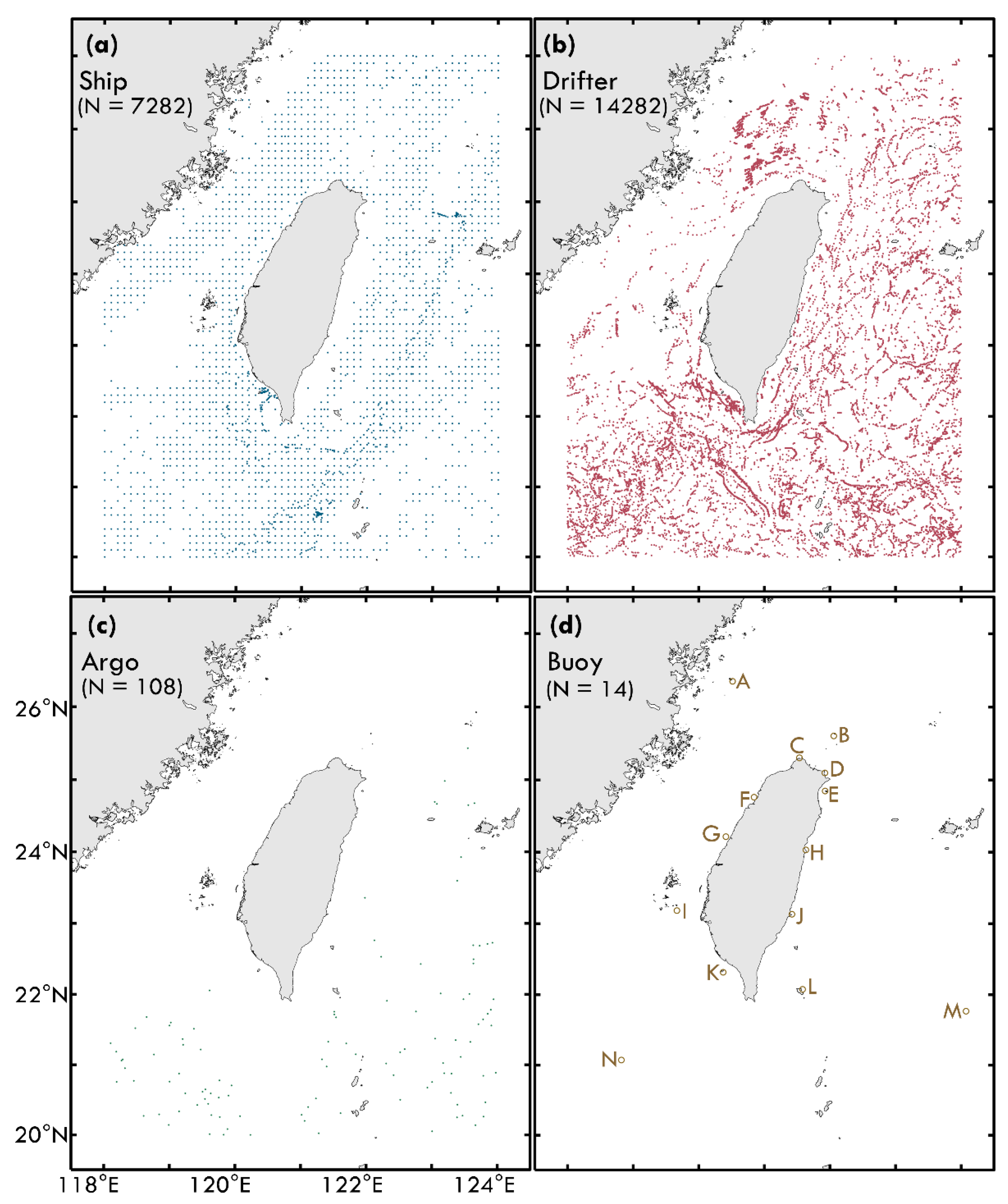
Historical in situ observation data and cloud-free Himawari-8 satellite data at the same location provide valuable comparative data to analyze the difference between bulk and skin SST. In addition to the differences in the instruments, the three in situ observations have different characteristics. Commercial ships have a fixed channel, the observation positions are mostly repeated, and the data points are widely and uniformly distributed. The drifter can move with the ocean current, and it can observe the SST variations in continuous close-up positions, with more than 10,000 comparable data. The observation time interval of Argo data is relatively long, and the instruments released into the ocean are also rare. There are only 108 samples in this study (Figure 2). Therefore, the analysis in this section focuses on ship and drifter data for comparison on the monthly and hourly time scales. The total number of data samples is presented in Table 1, and the sample numbers of individual data in each month are presented in Appendix A, Table A1.
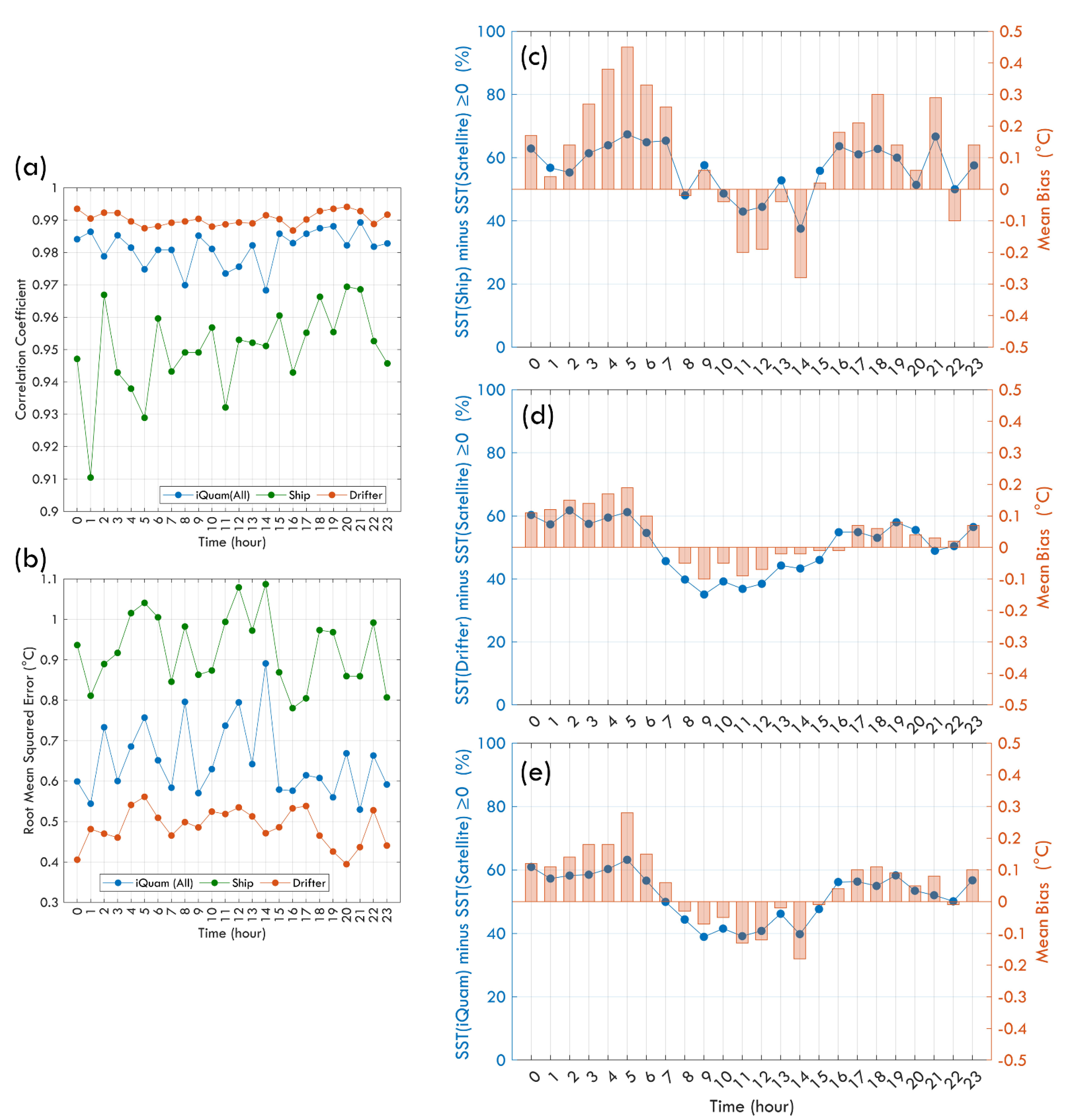
Figure 3a presents the correlation coefficient between the bulk and skin SST in each month, as well as the standard deviation (STD) of the ship and drifter data, to understand the difference in the monthly average spatial distribution scale. The monthly STD range of the ship SST was between 0.97 °C (August) and 3.40 °C (February), while the STD range of the drifter SST was between 0.84 °C (August) and 4.16 °C (February). Except for February, the STD of the ship SST was larger than the drifter SST each month, which may be due to SST measurements from commercial ships being much less accurate than those from drifters. Under the long-term scale and wide spatial range, the relation between ship bulk SST and skin SST was highly correlated with correlation coefficients, 0.9509 (ship) and 0.9901 (drifter); however, the root mean squared errors (RMSEs) of the two bulk SST dataset and skin SST dataset were quite different (ship: 0.9649 °C; drifter: 0.4924 °C). The mean bias were similar (Figure 3c–e), which were 0.03 ± 0.96 °C (ship) and 0.03 ± 0.49 °C (drifter). These results show that the difference between ship bulk SST and skin SST was much larger than that of drifter bulk SST, but the ratio of bulk SST minus skin SST greater than zero was almost the same (ship: 52%, drifter: 49%), resulting in the mean bias of the two being close. The maximum and minimum biases of ship bulk SST and skin SST were 3.64 °C and −4.95 °C, respectively, while those of drifter bulk SST were 3.15 °C and −2.92 °C, respectively.
The bias between bulk and skin SST has seasonal variation, which cannot be found if only the RMSE results are considered (Figure 3b). The correlations of bulk and skin SST were highest in spring and gradually decreased in July and August. The bias also changed from positive values in winter to negative values in summer (Figure 3c–e). Such results show that the strong solar insolation in summer leads to a significant stratification of the near-surface ocean, making the average bulk SST lower than the skin SST. In March, the wind speed in the ocean adjacent to Taiwan is weak, and the solar radiation is not as high as that in summer. Currently, the well-mixed near-surface ocean layer causes the average bulk SST to be slightly higher than the skin SST. The time series comparison of bulk and skin SST at the local time is shown in Figure 4. The high correlation represents the consistency of data within the hour (Figure 4a). As a result of the monthly timescale, the drifter SST and skin SST are closer than the ship SST and skin SST, and the daily variation is still not visible from the RMSE results (Figure 4b). However, the mean bias results show significant diurnal variation. During the daytime, especially near noon, the sea surface is affected by solar insolation and absorbs heat energy so the average bulk SST was lower than the skin SST. During the daytime, the mean bias of the ship SST was −0.13 °C and the drifter SST was −0.06 °C. The cool skin layer appears obviously at night, and the average bulk SST was higher than the skin SST. At night, the mean bias of ship SST was 0.20 °C and the drifter was 0.10 °C. The bias was greatest between four and five o’clock in the morning before the sun rose.
Additionally, according to Argo data, its correlation with skin SST was highly correlated (r = 0.9761), and the RMSE between Argo SST and skin SST was 0.46 °C, which is close to the result of the drifter SST, but the mean bias was −0.11 ± 0.45 °C, and the proportion of Argo SST minus a skin SST greater than zero was only 31.5%. The possible reason for this is that the bulk SST of Argo was the nominal surface temperature (0~5 m), which was slightly deeper than the sea temperature measured by the ship and the drifter. According to the near-surface oceanic temperature gradient vertical profile in the daytime, the sea temperature at ~5 m is lower than the skin SST and SST (~1 m), and the difference is small at night. The results show that the average bias of the Argo bulk SST and skin SST was −0.23 °C (n = 48) during the daytime and −0.01 °C (n = 60) during the nighttime.
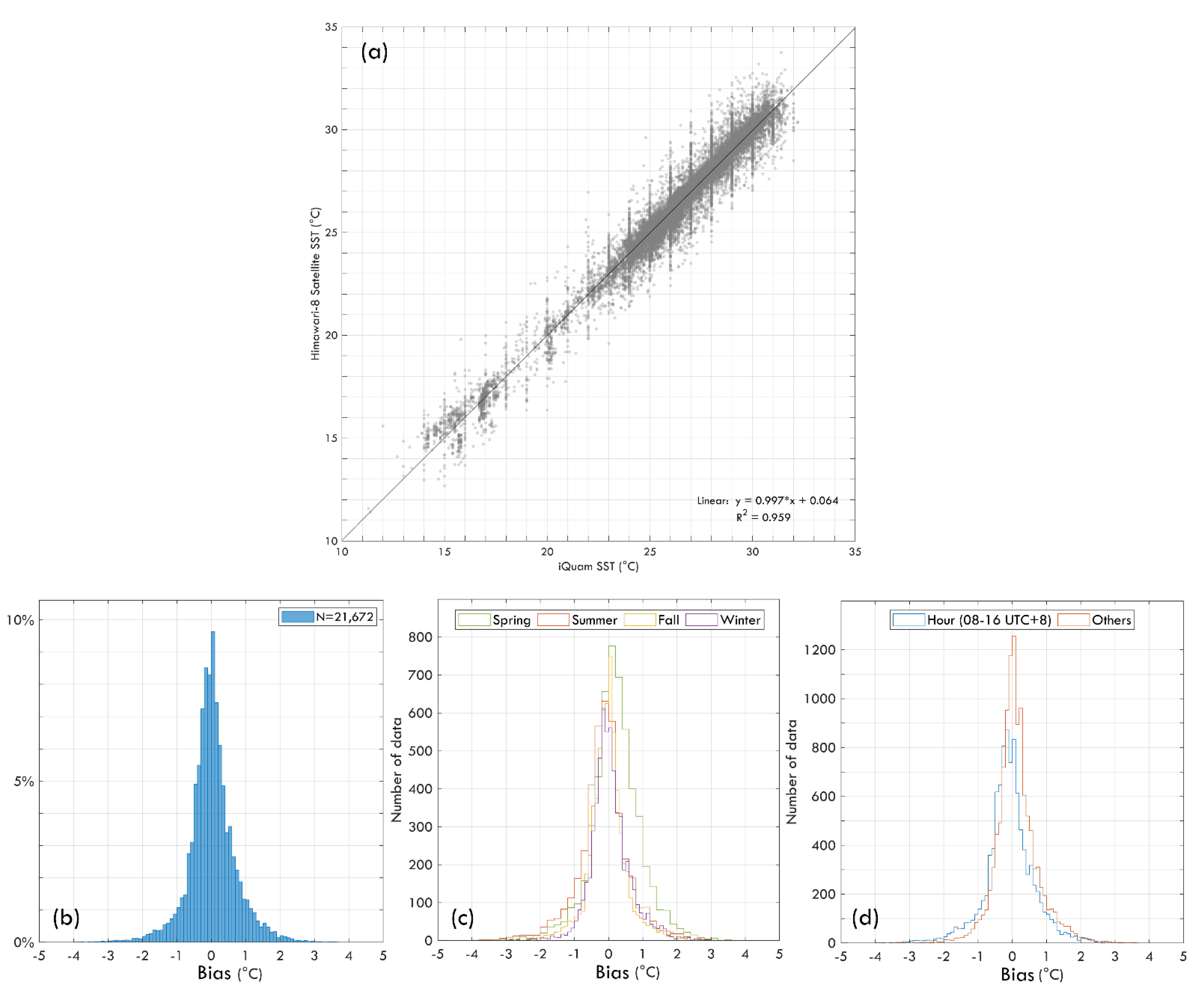
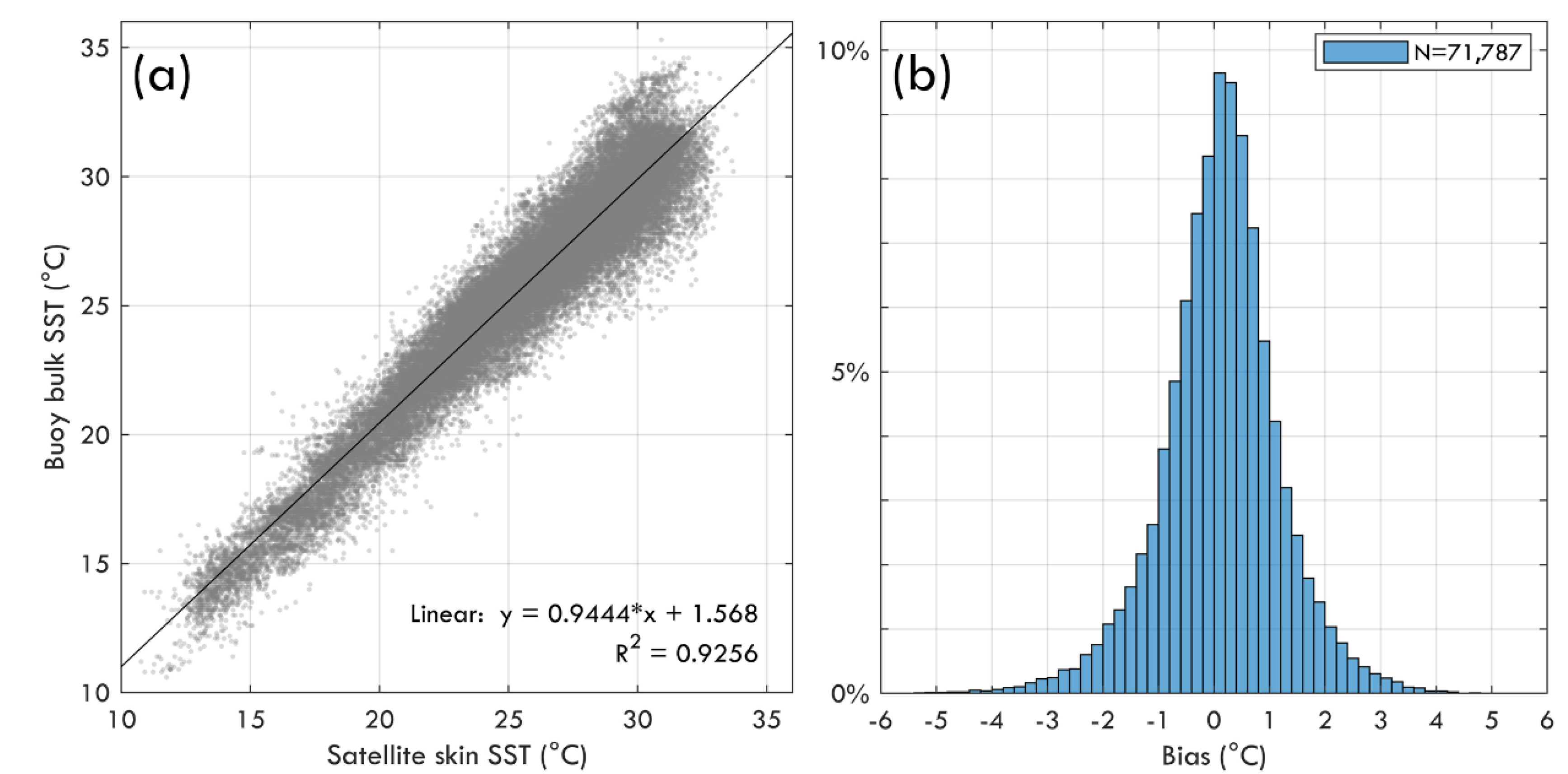
The long-term comparison between iQuam bulk SST and Himawari-8 skin SST had a high correlation, with a coefficient determination of 0.959. The average SST in this study area was 26.38 °C (bulk SST) and 26.35 °C (skin SST), and the mean bias was only 0.03 °C (Figure 5a). It is worth noting here that the comparison between bulk SST and skin SST is a concept of the probability distribution. In the total number of 21,672 samples of data, mean bias results accounted for 77.1% within one SD and 93.8% within two SD, accounting for 98.4% within three SD; therefore, the mean bias is used to illustrate whether the bias of bulk and skin SST tends to have a positive or negative value. According to the estimation of the near-surface SST vertical stratification model, solar insolation is obviously an important factor affecting the variation in bias on the diurnal and monthly scales (Figure 5c,d). However, there are no real-time wind speed data from these iQuam observation datasets. Therefore, there is no way to examine the combined effects of wind speed and insolation and the possibility of DWL generation.
3.2. Comparison of Satellite Skin SST and Buoy Bulk SST at a Fixed Position on Monthly and Diurnal Timescales
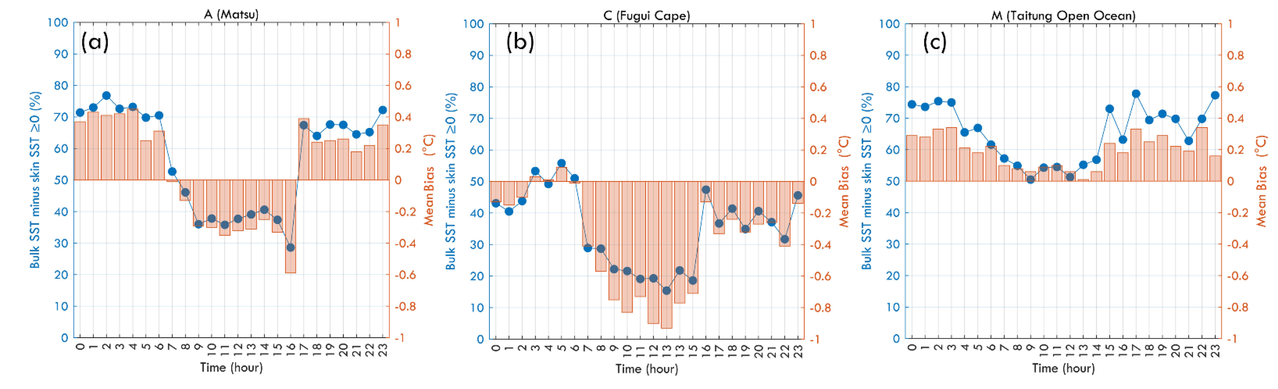
Different from the observed distributions of the random locations in the previous section, this section discusses the buoy data for 14 fixed sites (Figure 1b). Because each sea area has different ocean stratification conditions and hydrological characteristics, the variables affecting the near-surface temperature gradient can be controlled using fixed location sites. In general, RMSE results are used to evaluate the difference between the two SST sets. Figure 6a shows that the average RMSE of Groups I and II was less than 1 °C, and the RMSE of Group III was higher than 1 °C. Group III, which is close to the shore, could have been affected by river discharge, resulting in larger changes in SST. However, a difference in the near-surface temperature could not be found in the RMSE results. From the correlation between bulk and skin SST in each month (Figure 6b), it was found that the SST change at each buoy in the same month was large and inconsistent, which is the same as the results in Figure 3a. The mean bias value change of each buoy on a monthly timescale is shown in Figure A1. Figure 4 shows that the mean bias value change of the ship and the drifter on a daily scale was a typical skin effect. However, according to the 14 buoys, it seems that there was no obvious skin effect in the long-term average statistical results of some locations. Figure 7a shows the typical cool skin layer produced by the well-mixed near-surface layer at night and the DWL produced by the solar insolation during the daytime. In addition to A (Matsu), Buoys B, D, E, F, G, H, K, and L all had the same diurnal variation characteristics of mean bias. Figure 7b shows that even at nighttime, most of the bulk SST data were lower than the skin SST data, and the SST bias was even larger near noon. In addition to B (Fugui Cape), J (Cheng-Kung) also had such characteristics. Figure 7c shows that even in the daytime, the SST bias was still not quite different (Buoys M and N), and I (Chimi) even observed that the bulk SST was higher than the skin SST by more than 0.6 °C on average, no matter the time.
The above-mentioned skin effect was mainly caused by wind blowing on the sea surface and solar insolation. The time series data of the three buoys were used as examples of the possibility of the observed cool skin layer and the DWL (Figure 8). The SST time series in Figure 8a shows that skin SST was almost higher than bulk SST in three days, with a maximum bias of up to 2 °C. The Beaufort wind force scale changed from Level 4 to Level 1–2. Light winds caused the appearance of the DWL, and it would have been more significant in the case of strong shortwave radiation at noon. It is obvious from the bias diagrams of the two SSTs that such diurnal variation can be seen. Figure 8b shows the case of the impact of the rapid change in wind speed on the stratification of near-surface temperature. The wind speed changed from a Beaufort Scale 7 to 2–3 over four days. Strong winds caused seawater to mix well, making bulk SST higher than skin SST, thus producing a cool skin layer. Even at noon with strong solar insolation, bulk SST was still approximately 1 °C higher than skin SST. When the wind speed weakened, the water temperature immediately reacted. The obvious DWL caused the bulk SST to be 0.5 °C lower than the skin SST under strong shortwave radiation and created light wind conditions (2016/02/09 12:00 UTC+8). Figure 8c clearly shows the situation of the DWL on each of these five days. The strong solar insolation and the weak wind based on the Beaufort scale, 2–3 levels, caused 0.6 °C of the near-surface layer to be stratified. When there was no sunlight at night, the DWL disappeared. When the solar shortwave radiation weakened, the SST bias at noon may have also decreased; there was only a SST bias of 0.4 °C at 12:00 on 4 January 2017.
3.3. Effects of Wind and Solar Insolation on the Ocean Near-Surface Temperature Layer
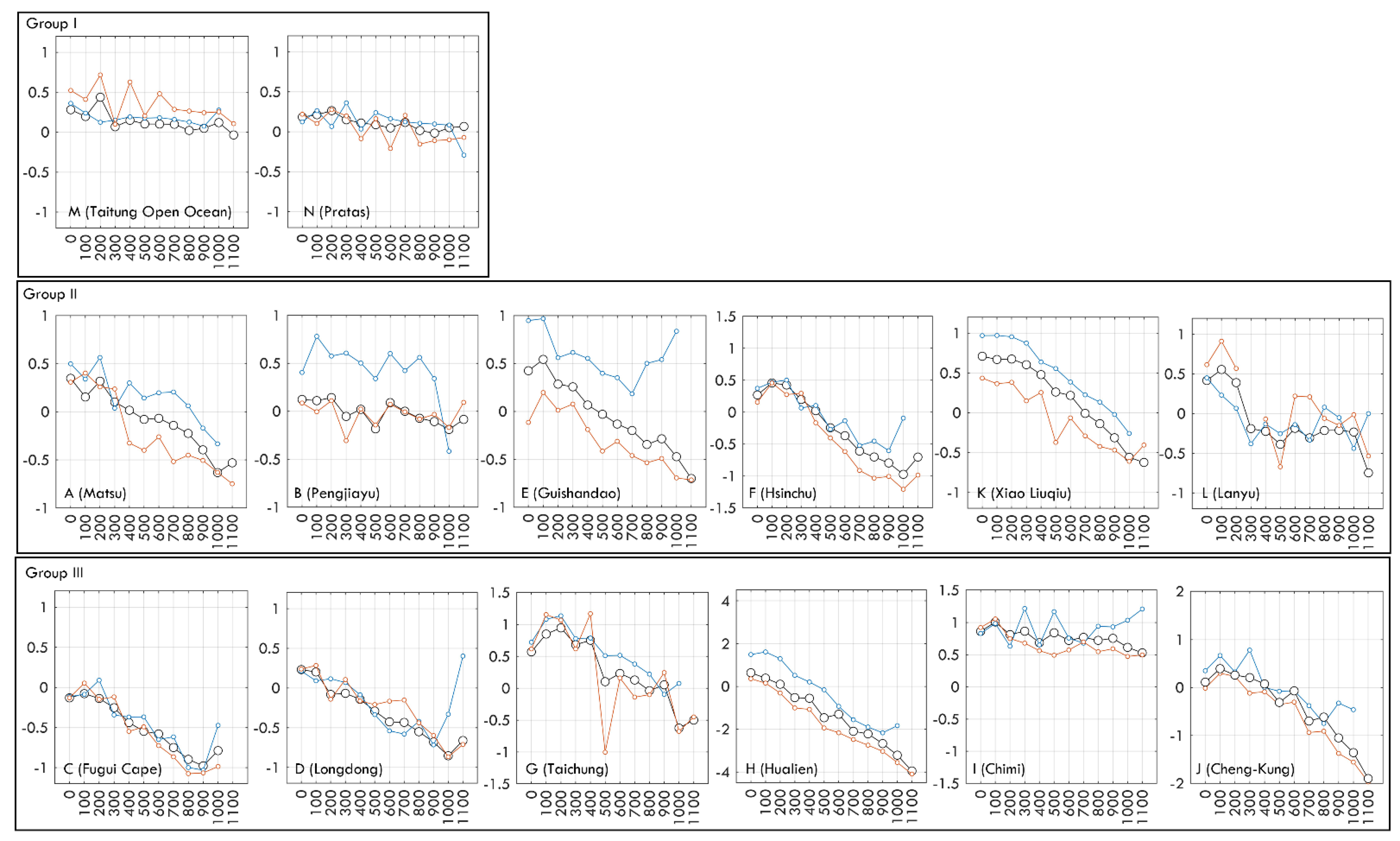
How much does the intensity of sunlight and wind speed affect the mixing and stratification of the ocean near the surface? First, the influence of solar shortwave radiation energy intensity on near-surface temperature is considered. The black dotted line in Figure 9 shows the variation in SST bias (bulk SST minus skin SST) observed by 14 buoys with the magnitude shortwave radiation at night and during the day. The results of 10 buoys show that the SST bias increased gradually with stronger shortwave radiation and could have formed a significant DWL. The SST bias feedback to the shortwave radiation at each buoy position was not the same. The shortwave radiation required for the difference between bulk and skin SST to change from a negative to a positive value was different at each position. This could have been related to the near-surface ocean structure of the water body at the location, or it may have been influenced by near-shore river runoff and other external factors. The skin SSTs of F (Hsinchu), H (Hualien), and J (Cheng-Kung) were strongly affected by shortwave radiation. Shortwave radiation exceeding 900 W/m2 caused the average SST bias to exceed 1 °C, while shortwave radiation exceeding 700 W/m2 caused the average SST bias of H (Hualien) to exceed 2 °C. However, for M (Taitung) and N (Pratas) in the open ocean and B (Pengjiayu), which was relatively far from Taiwan, the SST bias did not change significantly with shortwave radiation. At the I (Chimi) station, no matter how the solar radiation intensity changed, the bulk SST was higher than the skin SST. Will the same solar shortwave radiation intensity affect the near-surface temperature stratification in summer and winter? Usually, SST was lower and the mixed layer was thicker in the winter, whereas SST was relatively higher and the mixed layer was thinner in summer. The blue and red dotted lines in Figure 9 represent winter (December–March) and summer (June–September), respectively. The SST bias of some buoys (B, E, K, and H) had a significant seasonal variation in tiny shortwave radiation. The SST bias of some buoys (A, F, G, I, and J) caused the difference between summer and winter only after exceeding a certain threshold of shortwave radiation intensity. The SST bias of other stations (C, D, L, M, and N) had no obvious difference.
Next, the effect of ocean wind speed on the near-surface temperature was considered. Figure 10 shows the SST bias at each buoy position with the Beaufort wind force scale. The blue dotted line represents the nighttime situation; that is, the solar shortwave radiation was zero; and the orange dotted line indicates the daytime. Theoretically, at night and with strong wind, the near-surface seawater is well mixed, and the bulk SST is usually slightly higher than the skin SST, forming a cool skin layer. In the daytime and when the wind speed is weak, the near-surface water will be stratified, and the bulk SST will generally be slightly lower than the skin SST, forming a DWL. Taking the observation results of the A (Matsu) buoy as an example, when the wind speed was weak at night, the bulk and skin SSTs were almost the same. With the increase in wind speed, the cool skin layer and seawater were well mixed, resulting in the fact that when the Beaufort scale reached Level 6, the bulk SST was 0.8 °C higher than the skin SST. The A (Matsu) buoy observed a significant DWL in the daytime when the wind speed was weak. The bulk SST was 0.9 °C lower than the skin SST. With the increase in wind speed, the ocean near-surface stratification began to weaken and the vertical mixing increased. When the Beaufort scale reached Level 5, the average bulk and skin SSTs showed no difference. When the wind speed reached Level 6, the situation reversed such that the bulk SST was 0.4 °C higher than the skin SST. In the daytime, the same wind speed but different solar intensities could have changed the near-surface temperature gradient. In the case of A (Matsu) and in the low wind speed interval, the SST bias was 0.8 °C higher at higher solar insolation intensity (>500 W/m2) than at lower solar insolation intensity (<500 W/m2). Except for M (Taitung) and N (Pratas), which were located in the open ocean, and I (Chimi), the buoys observed that the near-surface temperature was affected by shortwave radiation under the same wind speed. As emphasized above, the characteristic conditions of the sea water at the location of the buoys could affect the impact of wind speed and solar insolation on the near-surface temperature structure. For example, when the Beaufort scale reached Level 5 or above in the daytime, F (Hsinchu), and G (Taichung) were observed to have significant vertical mixing that gradually replaced stratification.
4. Discussion
Four different in situ observation instruments and the Himawari-8 data were used to form an SST pair to analyze the differences in near-surface ocean temperature. Ship, drifter, and buoy represent the bulk SST at 1–2 m, while Argo’s bulk SST was close to 5 m, and satellite data represent skin SST. Different from previous studies that focused on the continuous observation of changes at a specific location over a short period or which considered the average error over a large area, this study emphasizes the examination of changes at different observation locations over a long period. The sample in this study was based on the weather in a clear sky, the observation time from an hourly scale to monthly and seasonal scales, the interval of wind speed, and the shortwave radiation intensity, distinguished to understand how the bulk SST and skin SST interacted with each other, to understand the possibility of cool skin, and the DWL caused by the vertical mixing and stratification of near-surface seawater. Table 3 summarizes the statistical results of various SST pairs. From the correlation coefficient, RMSE, and mean bias value, one may think that there was little difference between bulk and skin SST from these calculation methods, but this study noted the existence of a rapidly changing near-surface temperature gradient. Table 4 summarizes the maximum and minimum values of bias and the values of the 5th, 10th, 90th, and 95th percentiles of the SST pair in each dataset. It is speculated that these extreme values may have been caused by cloud sheet or river runoff near the shore. Figure 5 and Figure 11 show the scatter plots of these SST pairs and the distribution of the positive and negative values of SST bias, most of which are distributed between ±1.1 °C, and finally, a tiny mean bias value was calculated. However, the difference between bulk and skin SST is an important key to analyzing the depth of bulk SST, near-surface temperature stratification, and surface mixed layer. Additionally, previous studies have usually used local time to examine the impact of solar insolation on near-surface temperature. This study suggests that solar shortwave radiation data should be used instead of time as much as possible, which not only has an objective judgment standard but also ensures that the analysis and examination are conducted under the same solar energy. A significant DWL was not found in some buoy results (Figure 9 and Figure 10), and there is no clear evidence to say whether less frequent DWL events had occurred in some areas. What should be considered is the spatial difference between a buoy in a satellite grid point (2 × 2 km); whether there would be obvious changes in the hydrological characteristics within a 4 km2 of some locations still needs to be confirmed by sufficient data. Future researchers on this topic are strongly suggested to use satellite data to clarify SST changes before conducting surveys.
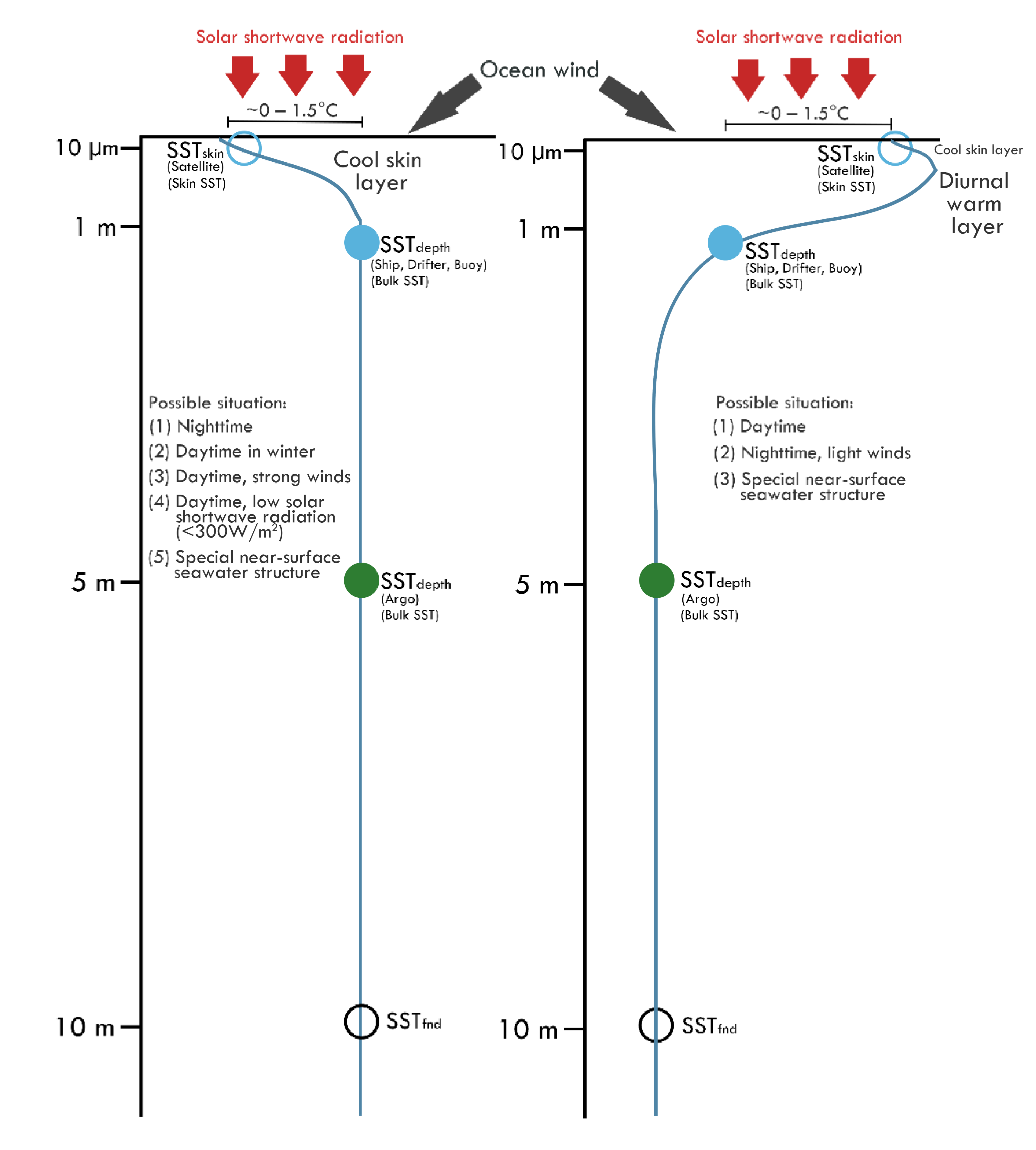
5. Summary
In this study, the bulk SST data from four different in situ observation instruments and the skin SST data from the geostationary Himawari-8 satellite were used to analyze the variation in the near-surface temperature gradient in Taiwan’s adjacent waters from July 2015 to May 2022, with a total of 93,459 SST pairs. On a long-term scale, the bulk SST was highly correlated with the skin SST, with an RMSE of 0.99 °C. The mean bias value was close to 0 °C because the wind speed and solar insolation jointly controlled the skin effect of the near-surface temperature structure, which caused the diurnal cycle of the cool skin layer and DWL to appear. On an hourly timescale, 80% of the SST pair bias was in the −1.04~1.25 °C range, and 90% of the SST pair bias was in the −1.55~1.71 °C range. Combining the SST pairs, the solar shortwave radiation data, the buoy ocean wind speed data, and the variation in the difference between bulk and skin SSTs under different air-sea conditions were successfully analyzed. The reason why bulk SST was higher than skin SST was that the near-surface seawater was well mixed (Figure 12), which mainly occurred in (1) nighttime, (2) daytime in winter, (3) daytime with strong winds, and (4) daytime but with low solar shortwave radiation (<300 W/m2). The reason why bulk SST was lower than skin SST was that the near-surface seawater was stratified significantly (Figure 12), which mainly occurred in (1) daytime and (2) nighttime with light winds. However, the special near-surface ocean structure of some sea areas may not have followed the above rules and may have been observed as a cool skin layer and DWL. In conclusion, combining geostationary Himawari-8 satellite data with in situ observation data can effectively analyze the multitemporal and spatial near-surface temperature variations, and this can be combined with a cruise to further understand other near-surface ocean dynamic issues.
Funding
This work was supported by the Ministry of Science and Technology of Taiwan through grant 110-2611-M-008-007 and 111-2611-M-008-007.
Data Availability Statement
The iQuam dataset was obtained from https://www.star.nesdis.noaa.gov/socd/sst/iquam/data.html (accessed on 13 September 2022). The CWB dataset was obtained from the Safe Ocean (https://ocean.cwb.gov.tw/V2/ (accessed on 13 September 2022)). The Himawari satellite-derived skin SST and shortwave radiation data was obtained from the JAXA p-tree system (https://www.eorc.jaxa.jp/ptree/index.html (accessed on 13 September 2022)).
Acknowledgments
The author appreciates all the data used, provided from open databases. The author thanks anonymous reviewers and academic editors for their comments.
Conflicts of Interest
The author declares no conflict of interest.
Appendix A

Table A1.
The amount of data of each observation measurements of iQuam in each month.
| Jan. | Feb. | Mar. | Apr. | May. | Jun. | Jul. | Aug. | Sep. | Oct. | Nov. | Dec. | |
|---|---|---|---|---|---|---|---|---|---|---|---|---|
| All | 1514 | 3220 | 2938 | 1419 | 960 | 995 | 1990 | 1070 | 1787 | 2336 | 2237 | 1206 |
| Ship | 387 | 550 | 756 | 713 | 544 | 455 | 737 | 601 | 638 | 1014 | 600 | 287 |
| Drifter | 1117 | 2658 | 2171 | 695 | 411 | 535 | 1249 | 462 | 1141 | 1310 | 1619 | 914 |
| Argo | 10 | 12 | 11 | 11 | 5 | 5 | 4 | 7 | 8 | 12 | 18 | 5 |
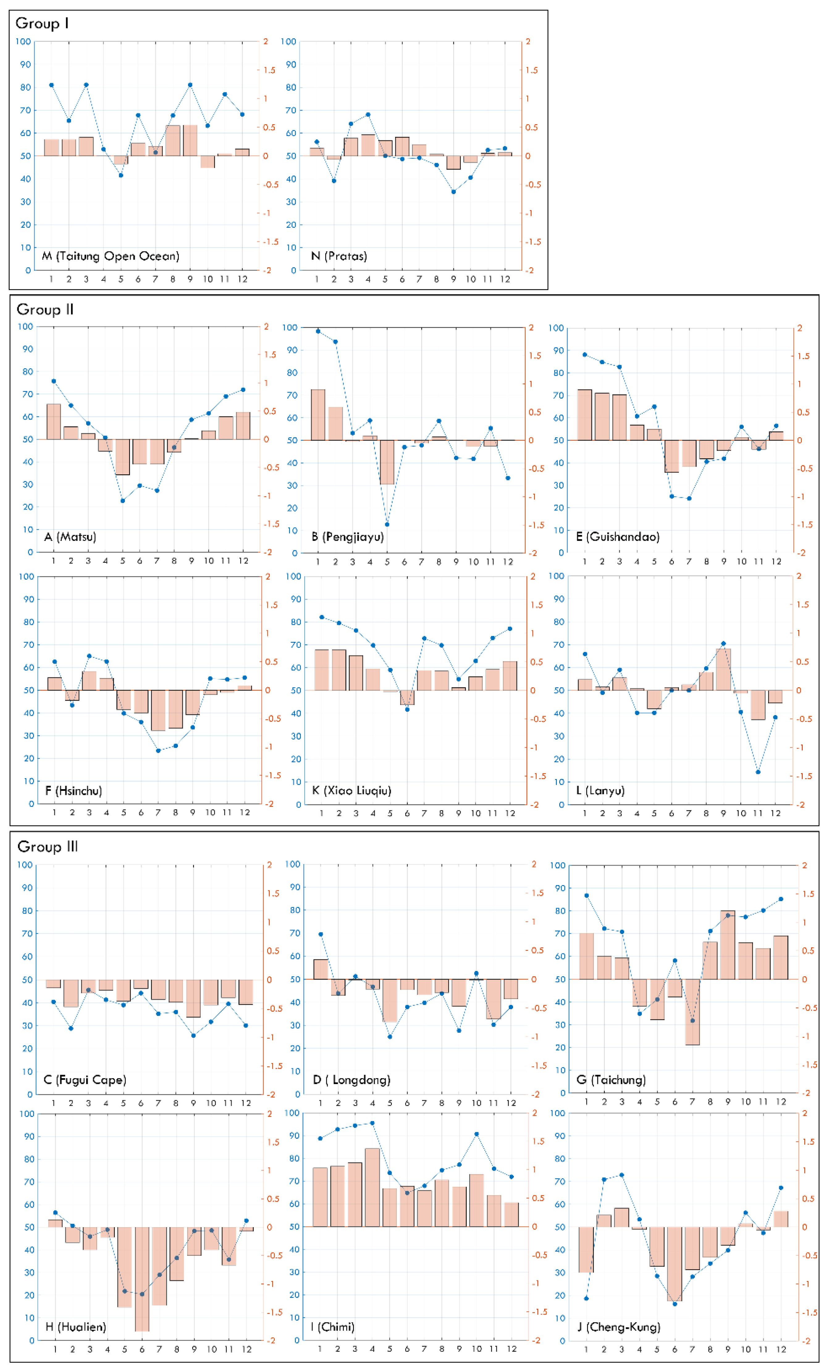
Figure A1.
The difference between each buoy bulk SST and satellite skin SST in each month. The left vertical axis represents the percentage of data that bulk SST is greater than skin SST, and the right vertical axis represents the mean bias.
Figure A1.
The difference between each buoy bulk SST and satellite skin SST in each month. The left vertical axis represents the percentage of data that bulk SST is greater than skin SST, and the right vertical axis represents the mean bias.

References
- Donlon, C.; Robinson, I.; Casey, K.S.; Vazquez-Cuervo, J.; Armstrong, E.; Arino, O.; Gentemann, C.; May, D.; LeBorgne, P.; Piollé, J.; et al. The global ocean data assimilation experiment high-resolution sea surface temperature pilot project. Bull. Am. Meteorol. Soc. 2007, 88, 1197–1214. [Google Scholar] [CrossRef]
- Barton, I.J. Interpretation of satellite-derived sea surface temperatures. Adv. Space Res. 2001, 28, 165–170. [Google Scholar] [CrossRef]
- Minnett, P.J. Radiometric measurements of the sea-surface skin temperature: The competing roles of the diurnal thermocline and the cool skin. Int. J. Remote Sens. 2003, 24, 5033–5047. [Google Scholar] [CrossRef]
- Ward, B. Near-surface ocean temperature. J. Geophys. Res. Oceans 2006, 111, C02004. [Google Scholar] [CrossRef] [Green Version]
- Gentemann, C.L.; Minnett, P.J. Radiometric measurements of ocean surface thermal variability. J. Geophys. Res. Oceans 2008, 113, C08017. [Google Scholar] [CrossRef] [Green Version]
- Murray, M.J.; Allen, M.R.; Merchant, C.J.; Harris, A.R.; Donlon, C.J. Direct observations of skin-bulk SST variability. Geophys. Res. Lett. 2000, 27, 1171–1174. [Google Scholar] [CrossRef] [Green Version]
- Alappattu, D.P.; Wang, Q.; Yamaguchi, R.; Lind, R.J.; Reynolds, M.; Christman, A.J. Warm layer and cool skin corrections for bulk water temperature measurements for air-sea interaction studies. J. Geophys. Res. Oceans 2017, 122, 6470–6481. [Google Scholar] [CrossRef]
- Ruiz-de la Torre, M.C.; Maske, H.; Ochoa, J.; Almeda-Jauregui, C.O. Maintenance of coastal surface blooms by surface temperature stratification and wind drift. PLoS ONE 2013, 8, e58958. [Google Scholar] [CrossRef]
- Zhang, H.; Babanin, A.V.; Liu, Q.; Ignatov, A. Cool skin signals observed from Advanced Along-Track Scanning Radiometer (AATSR) and in situ SST measurements. Remote Sens. Environ. 2019, 226, 38–50. [Google Scholar] [CrossRef]
- Zhang, H.; Beggs, H.; Ignatov, A.; Babanin, A.V. Nighttime cool skin effect observed from Infrared SST Autonomous Radiometer (ISAR) and depth temperatures. J. Atmos. Ocean. Technol. 2020, 37, 33–46. [Google Scholar] [CrossRef]
- Zhang, R.; Zhou, F.; Wang, X.; Wang, D.; Gulev, S.K. Cool skin effect and its impact on the computation of the latent heat flux in the South China Sea. J. Geophys. Res. Oceans 2021, 126, 2020JC016498. [Google Scholar] [CrossRef]
- Wong, E.W.; Minnett, P.J. The response of the ocean thermal skin layer to variations in incident infrared radiation. J. Geophys. Res. Oceans 2018, 123, 2475–2493. [Google Scholar] [CrossRef]
- Hughes, K.G.; Moum, J.N.; Shroyer, E.L. Evolution of the velocity structure in the diurnal warm layer. J. Phys. Oceanogr. 2020, 50, 615–631. [Google Scholar] [CrossRef]
- Hughes, K.G.; Moum, J.N.; Shroyer, E.L. Heat transport through diurnal warm layers. J. Phys. Oceanogr. 2020, 50, 2885–2905. [Google Scholar] [CrossRef]
- Hughes, K.G.; Moum, J.N.; Shroyer, E.L.; Smyth, W.D. Stratified shear instabilities in diurnal warm layers. J. Phys. Oceanogr. 2021, 51, 2583–2598. [Google Scholar] [CrossRef]
- Gille, S.T. Diurnal variability of upper ocean temperatures from microwave satellite measurements and Argo profiles. J. Geophys. Res. Oceans 2012, 117, C11027. [Google Scholar] [CrossRef] [Green Version]
- Prytherch, J.; Farrar, J.T.; Weller, R.A. Moored surface buoy observations of the diurnal warm layer. J. Geophys. Res. Oceans 2013, 118, 4553–4569. [Google Scholar] [CrossRef] [Green Version]
- Matthews, A.J.; Baranowski, D.B.; Heywood, K.J.; Flatau, P.J.; Schmidtko, S. The surface diurnal warm layer in the Indian Ocean during CINDY/DYNAMO. J. Clim. 2014, 27, 9101–9122. [Google Scholar] [CrossRef] [Green Version]
- Zhu, X.; Minnett, P.J.; Berkelmans, R.; Hendee, J.; Manfrino, C. Diurnal warming in shallow coastal seas: Observations from the Caribbean and Great Barrier Reef regions. Cont. Shelf Res. 2014, 82, 85–98. [Google Scholar] [CrossRef]
- Minnett, P.J.; Kilpatrick, K.A.; Podestá, G.P.; Evans, R.H.; Szczodrak, M.D.; Izaguirre, M.A.; Williams, E.J.; Walsh, S.; Reynolds, R.M.; Bailey, S.W.; et al. Skin sea-surface temperature from VIIRS on Suomi-NPP—NASA continuity retrievals. Remote Sens. 2020, 12, 3369. [Google Scholar] [CrossRef]
- Chung, H.W.; Liu, C.C. Spatiotemporal variation of cold eddies in the upwelling zone off northeastern Taiwan revealed by the geostationary satellite imagery of ocean color and sea surface temperature. Sustainability 2019, 11, 6979. [Google Scholar] [CrossRef] [Green Version]
- Yin, W.; Huang, D. Short-term variations in the surface upwelling off northeastern Taiwan observed via satellite data. J. Geophys. Res. Oceans 2019, 124, 939–954. [Google Scholar] [CrossRef]
- Yin, W.; Ma, Y.; Wang, D.; He, S.; Huang, D. Surface Upwelling off the Zhoushan Islands, East China Sea, from Himawari-8 AHI Data. Remote Sens. 2022, 14, 3261. [Google Scholar] [CrossRef]
- Hsu, P.C.; Lee, H.J.; Zheng, Q.; Lai, J.W.; Su, F.C.; Ho, C.R. Tide-Induced Periodic Sea Surface Temperature Drops in the Coral Reef Area of Nanwan Bay, Southern Taiwan. J. Geophys. Res. Oceans 2020, 125, e2019JC015226. [Google Scholar] [CrossRef]
- Hsu, P.C.; Ho, C.Y.; Lee, H.J.; Lu, C.Y.; Ho, C.R. Temporal variation and spatial structure of the Kuroshio-induced submesoscale island vortices observed from GCOM-C and Himawari-8 data. Remote Sens. 2020, 12, 883. [Google Scholar] [CrossRef] [Green Version]
- Hu, Z.; Xie, G.; Zhao, J.; Lei, Y.; Xie, J.; Pang, W. Mapping Diurnal Variability of the Wintertime Pearl River Plume Front from Himawari-8 Geostationary Satellite Observations. Water 2021, 14, 43. [Google Scholar] [CrossRef]
- Tu, Q.; Hao, Z. Validation of Sea Surface Temperature Derived From Himawari-8 by JAXA. IEEE J. Sel. Top. Appl. Earth Obs. Remote Sens. 2020, 13, 448–459. [Google Scholar] [CrossRef]
- Wirasatriya, A.; Hosoda, K.; Setiawan, J.D.; Susanto, R.D. Variability of diurnal sea surface temperature during short term and high SST event in the western equatorial pacific as revealed by satellite data. Remote Sens. 2020, 12, 3230. [Google Scholar] [CrossRef]
- Yang, Y.C.; Lu, C.Y.; Huang, S.J.; Yang, T.Z.; Chang, Y.C.; Ho, C.R. On the Reconstruction of Missing Sea Surface Temperature Data from Himawari-8 in Adjacent Waters of Taiwan Using DINEOF Conducted with 25-h Data. Remote Sens. 2022, 14, 2818. [Google Scholar] [CrossRef]
- Yang, M.; Guan, L.; Beggs, H.; Morgan, N.; Kurihara, Y.; Kachi, M. Comparison of Himawari-8 AHI SST with shipboard skin SST measurements in the Australian region. Remote Sens. 2020, 12, 1237. [Google Scholar] [CrossRef]
- Xu, F.; Ignatov, A. In situ SST quality monitor (iQuam). J. Atmos. Ocean. Technol. 2014, 31, 164–180. [Google Scholar] [CrossRef]
- Kurihara, Y.; Murakami, H.; Kachi, M. Sea surface temperature from the new Japanese geostationary meteorological Himawari-8 satellite. Geophys. Res. Lett. 2016, 43, 1234–1240. [Google Scholar] [CrossRef] [Green Version]
- Kurihara, Y.; Murakami, H.; Ogata, K.; Kachi, M. A quasi-physical sea surface temperature method for the split-window data from the Second-generation Global Imager (SGLI) onboard the Global Change Observation Mission-Climate (GCOM-C) satellite. Remote Sens. Environ. 2021, 257, 112347. [Google Scholar] [CrossRef]
Figure 1.
(a) The study area and the long-term average ocean geostrophic currents from July 2015 to May 2022, (b) the long-term average SST derived by the Himawari-8 satellite from August 2015 to April 2022, and (c) the climatological monthly average SST from the Himawari-8 satellite at each station in Figure 1b from August 2015 to April 2022.

Figure 2.
The spatial distribution of four kinds of in situ observation data. (a) Ship, (b) drifter, (c) Argo, and (d) buoy.
Figure 2.
The spatial distribution of four kinds of in situ observation data. (a) Ship, (b) drifter, (c) Argo, and (d) buoy.

Figure 3.
Comparison of bulk SST and skin SST on a monthly time scale: (a) comparison of satellite skin SST and bulk SST of drifter and ship for each month, (b) the RMSE between skin SST and bulk SST, and the percentage of data that bulk SST is greater than skin SST and the mean bias between (c) ship and satellite, (d) drifter and satellite, and (e) iQuam dataset and satellite.

Figure 4.
Comparison of bulk SST and skin SST on hourly timescales: (a) the correlation between skin SST and bulk SST, (b) the RMSE between skin SST and bulk SST, and the percentage of data that bulk SST is greater than skin SST and the mean bias between (c) ship and satellite, (d) drifter and satellite, and (e) iQuam dataset and satellite.

Figure 5.
(a) Comparison of SST data between the iQuam and Himawari-8 satellite, and the histogram of bias for bulk-skin SST data pairs (b) for all samples, (c) in four seasons, and (d) during daytime and nighttime. A positive value of bias indicates that bulk SST (iQuam) is greater than skin SST (satellite).

Figure 6.
The (a) RMSE and (b) correlation between each buoy bulk SST and satellite skin SST on monthly time scales. The black dots (all data) refer to all bulk-skin SST pairs at each location. In addition, all the data at each location are divided into 12 months. The red and blue dots are the highest and lowest values on the monthly time scale, respectively.

Figure 7.
Three different types of bulk and skin SST diurnal variations. (a) The near-surface SST gradient had obvious diurnal variation, (b) ocean near-surface skin SST was more likely to be warmer than bulk SST, and (c) ocean near-surface skin SST was more likely to be cooler than bulk SST.
Figure 7.
Three different types of bulk and skin SST diurnal variations. (a) The near-surface SST gradient had obvious diurnal variation, (b) ocean near-surface skin SST was more likely to be warmer than bulk SST, and (c) ocean near-surface skin SST was more likely to be cooler than bulk SST.

Figure 8.
Time series variations of bulk and skin SST in (a) Hsinchu, (b) Chimi, and (c) Xiao Liuqiu, and their corresponding solar shortwave radiation and wind speed.
Figure 8.
Time series variations of bulk and skin SST in (a) Hsinchu, (b) Chimi, and (c) Xiao Liuqiu, and their corresponding solar shortwave radiation and wind speed.

Figure 9.
The effect of solar insolation on ocean near-surface temperature. The horizontal axis is solar shortwave radiation (W/m2), 0 represents nighttime radiation, and 100 represents shortwave radiation in a range of 0 to 100. The vertical axis is the bias of bulk SST minus skin SST (°C). The black line represents all data, the blue line is winter (December–March), and the red line is summer (June–September).

Figure 10.
The effect of wind speed on ocean near-surface temperature. The horizontal axis is the Beaufort wind force scale, where one represents a wind speed of 0.3–1.5 m/s and seven represents a wind speed of 13.9–17.1 m/s; the vertical axis is the bias of the bulk SST minus the skin SST (°C). The blue line represents the nighttime, the orange line is the daytime, the green line is the shortwave radiation less than 500 W/m2, and the red line is the shortwave radiation higher than 500 W/m2.

Figure 11.
(a) Comparison of SST data between buoys and the Himawari-8 satellite and (b) the histogram of bias for bulk-skin SST data pairs (b) for all samples.
Figure 11.
(a) Comparison of SST data between buoys and the Himawari-8 satellite and (b) the histogram of bias for bulk-skin SST data pairs (b) for all samples.

Figure 12.
Schematic diagram of the ocean near-surface temperature structure.

Table 1.
Number of bulk-skin SST data pairs obtained from the iQuam database from July 2015 to May 2022.
Table 1.
Number of bulk-skin SST data pairs obtained from the iQuam database from July 2015 to May 2022.
| Total | Commercial Ships | Drifting Buoys | Argo Floats |
|---|---|---|---|
| 21,672 | 7282 | 14,282 | 108 |
Table 2.
The ID, name, location, number of bulk-skin SST data pairs, distance from shore, and classification of 14 buoys from the CWB. Buoy stations are classified into Group I (open sea area), Group II (nearshore, bay, and island), and Group III (coastal area, estuary, and water channel).
Table 2.
The ID, name, location, number of bulk-skin SST data pairs, distance from shore, and classification of 14 buoys from the CWB. Buoy stations are classified into Group I (open sea area), Group II (nearshore, bay, and island), and Group III (coastal area, estuary, and water channel).
| ID | Name | Location | Number | Distance from Shore | Group |
|---|---|---|---|---|---|
| A | Matsu | 26°21′09″N, 120°30′55″E | 6577 | 1.4 km | II |
| B | Pengjiayu | 25°36′15″N, 122°03′31″E | 2290 | 2.9 km | II |
| C | Fugui Cape | 25°18′16″N, 121°32′03″E | 2593 | 650 m | III |
| D | Longdong | 25°05′52″N, 121°55′21″E | 1795 | 300 m | III |
| E | Guishandao | 24°50′55″N, 121°55′34″E | 5495 | 900 m * | II |
| F | Hsinchu | 24°45′46″N, 120°50′34″E | 11,632 | 4.8 km | II |
| G | Taichung | 24°12′56″N, 120°24′48″E | 4412 | 4.8 km ** | III |
| H | Hualien | 24°01′52″N, 121°37′57″E | 2945 | 300 m | III |
| I | Chimi | 23°11′02″N, 119°40′00″E | 8944 | 6.7 km *** | III |
| J | Cheng-Kung | 23°07′57″N, 121°25′13″E | 2268 | 600 m | III |
| K | Xiao Liuqiu | 22°18′58″N, 120°22′18″E | 10,099 | 1.15 km | II |
| L | Lanyu | 22°04′31″N, 121°34′58″E | 1088 | 350 m | II |
| M | Taitung Open Ocean | 21°45′59″N, 124°04′27″E | 3404 | **** | I |
| N | Pratas | 21°04′24″N, 118°49′12″E | 8245 | **** | I |
* In the bay. ** At the estuary of the river. *** In the water channel. **** In the open ocean.
Table 3.
Statistical results between bulk SST and skin SST; % represents the proportion of bulk SST higher than skin SST.
Table 3.
Statistical results between bulk SST and skin SST; % represents the proportion of bulk SST higher than skin SST.
| Data | R | RMSE (°C) | Mean Bias (°C) | % |
|---|---|---|---|---|
| Random point | ||||
| Ship | 0.9509 | 0.96 | 0.03 | 52.0 |
| Drifter | 0.9901 | 0.49 | 0.03 | 48.9 |
| Argo | 0.9761 | 0.46 | −0.11 | 31.5 |
| Fixed buoy (Group I) | ||||
| M (Taitung Open Ocean) | 0.9436 | 0.70 | 0.18 | 63.3 |
| N (Pratas) | 0.9350 | 0.79 | 0.13 | 50.4 |
| Fixed buoy (Group II) | ||||
| A (Matsu) | 0.9874 | 0.90 | 0.00 | 53.5 |
| B (Pengjiayu) | 0.9696 | 0.70 | 0.03 | 52.2 |
| E (Guishandao) | 0.9479 | 0.99 | 0.02 | 51.1 |
| F (Hsinchu) | 0.9798 | 0.96 | −0.14 | 48.0 |
| K (Xiao Liuqiu) | 0.9229 | 0.97 | 0.37 | 63.3 |
| L (Lanyu) | 0.8428 | 1.01 | 0.08 | 63.3 |
| Fixed buoy (Group III) | ||||
| C (Fugui Cape) | 0.9719 | 1.03 | −0.34 | 36.4 |
| D (Longdong) | 0.9637 | 1.05 | −0.27 | 41.2 |
| G (Taichung) | 0.9505 | 1.31 | 0.40 | 69.6 |
| H (Hualien) | 0.7583 | 1.88 | −0.74 | 40.1 |
| I (Chimi) | 0.9108 | 1.33 | 0.81 | 81.2 |
| J (Cheng-Kung) | 0.8563 | 1.14 | −0.38 | 41.2 |
Table 4.
Statistics of the bias between bulk SST and skin SST.
| 5th (°C) | 10th (°C) | 90th (°C) | 95th (°C) | Min. (°C) | Max. (°C) | |
|---|---|---|---|---|---|---|
| Ship | −1.61 | −1.16 | 1.21 | 1.62 | −4.95 | 3.64 |
| Drifter | −0.66 | −0.50 | 0.63 | 0.89 | −2.92 | 3.15 |
| Argo | −0.75 | −0.54 | 0.37 | 0.61 | −1.74 | 1.31 |
| A (Matsu) | −1.48 | −1.13 | 1.06 | 1.35 | −5.00 | 4.00 |
| B (Pengjiayu) | −1.13 | −0.76 | 0.79 | 1.12 | −3.30 | 3.19 |
| C (Fugui Cape) | −2.00 | −1.60 | 0.80 | 1.18 | −4.74 | 3.75 |
| D (Longdong) | −1.95 | −1.63 | 0.96 | 1.31 | −4.00 | 3.32 |
| E (Guishandao) | −1.60 | −1.20 | 1.28 | 1.69 | −4.96 | 4.21 |
| F (Hsinchu) | −1.80 | −1.43 | 0.97 | 1.26 | −4.00 | 5.72 |
| G (Taichung) | −1.96 | −1.17 | 1.72 | 2.75 | −4.41 | 4.83 |
| H (Hualien) | −3.75 | −3.14 | 1.40 | 1.77 | −6.28 | 3.20 |
| I (Chimi) | −0.83 | −0.40 | 2.22 | 2.61 | −3.44 | 4.74 |
| J (Cheng-Kung) | −2.33 | −1.90 | 0.83 | 1.13 | −6.84 | 4.38 |
| K (Xiao Liuqiu) | −1.11 | −0.72 | 1.45 | 1.75 | −5.11 | 3.41 |
| L (Lanyu) | −1.33 | −1.08 | 1.50 | 1.93 | −2.68 | 3.01 |
| M (Taitung Open Ocean) | −0.90 | −0.57 | 1.08 | 1.36 | −4.30 | 2.83 |
| N (Pratas) | −0.83 | −0.63 | 1.06 | 1.84 | −3.05 | 4.72 |
Publisher’s Note: MDPI stays neutral with regard to jurisdictional claims in published maps and institutional affiliations. |
© 2022 by the author. Licensee MDPI, Basel, Switzerland. This article is an open access article distributed under the terms and conditions of the Creative Commons Attribution (CC BY) license (https://creativecommons.org/licenses/by/4.0/).
Share and Cite
MDPI and ACS Style
Hsu, P.-C. Evaluation of Wind and Solar Insolation Influence on Ocean Near-Surface Temperature from In Situ Observations and the Geostationary Himawari-8 Satellite. Remote Sens. 2022, 14, 4975. https://doi.org/10.3390/rs14194975
AMA Style
Hsu P-C. Evaluation of Wind and Solar Insolation Influence on Ocean Near-Surface Temperature from In Situ Observations and the Geostationary Himawari-8 Satellite. Remote Sensing. 2022; 14(19):4975. https://doi.org/10.3390/rs14194975
Chicago/Turabian StyleHsu, Po-Chun. 2022. "Evaluation of Wind and Solar Insolation Influence on Ocean Near-Surface Temperature from In Situ Observations and the Geostationary Himawari-8 Satellite" Remote Sensing 14, no. 19: 4975. https://doi.org/10.3390/rs14194975
Note that from the first issue of 2016, this journal uses article numbers instead of page numbers. See further details here.