Article

Variability of Chl a Concentration of Priority Marine Regions of the Northwest of Mexico

by
Carlos Manuel Robles-Tamayo
1,
Ricardo García-Morales
2,*,
José Raúl Romo-León
3,
Gudelia Figueroa-Preciado
4,
María Cristina Peñalba-Garmendia
3 and
Luis Fernando Enríquez-Ocaña
3
1
Graduate Doctoral Program in Biosciences, University of Sonora, Hermosillo 83000, Mexico
2
Council of Science and Technology (CONACYT), Center for Biological Research of the Northwest S.C. Nayarit Unit (UNCIBNOR+), Tepic 63173, Mexico
3
Department of Scientifical and Technological Research, University of Sonora, Hermosillo 83000, Mexico
4
Department of Mathematics, University of Sonora, Hermosillo 83000, Mexico
*
Author to whom correspondence should be addressed.
Remote Sens. 2022, 14(19), 4891; https://doi.org/10.3390/rs14194891
Submission received: 2 September 2022 / Revised: 24 September 2022 / Accepted: 28 September 2022 / Published: 30 September 2022

Abstract

:
Priority Marine Regions (PMR) are important areas for biodiversity conservation in the Northwest Pacific Ocean in Mexico. The oceanographic dynamics of these regions are very important to understand their variability, generate analyses, and predict climate change trends by generating an adequate management of marine resources and their ecological characterization. Chlorophyll a (Chl a) is important to quantify phytoplankton biomass, consider the main basis of the trophic web in marine ecosystems, and determine the primary productivity levels and trends of change. The objective of this research is to analyze the oceanographic variability of 24 PMR through monthly 1-km satellite image resolution Chl a data from September 1997 to October 2018. A cluster analysis of Chl a data yielded 18 regions with clear seasonal variability in the Chl a concentration in the South-Californian Pacific (maximum values in spring-summer and minimum ones in autumn-winter) and Gulf of California (maximum values in winter-spring and minimum ones in summer-autumn). Significant differences (p < 0.05) were observed in Chl a concentration analyses for each one of the regions when climate patterns—El Niño/La Niña Southern Oscillation (ENSO) and normal events—were compared for all the seasons of the year (spring, summer, autumn, and winter).

Graphical Abstract

1. Introduction

In Mexico, diverse marine and coastal areas are characterized for their high levels of biodiversity because of the interaction between the ocean and atmosphere with a constant material-energy exchange in conjunction with geographical aspects [1]. Examples of these areas are the Baja California Peninsula and Gulf of California recognized as some of the most significant marine habitats rich in biota, such as marine mammals and sharks [2,3], Totoaba, and Marine Vaquita [4,5], respectively. Both marine areas have important and diverse species because of their primary productivity levels and conservation besides representing principal fishing zones of different species, such as shrimp, squid, and small (anchovy and sardine) and large (marlin and tuna) pelagic fishes [4,6,7].
This study aims to protect these environments and generate an adequate conservation and research management of their biodiversity. The National Biodiversity Commission (CONABIO, for its acronym in Spanish) determined some zones as Priority Marine Regions (PMR), considered important areas for biodiversity and natural resource conservation. Thus, these PMR were identified by analyzing environmental (biotic and abiotic) and economic (fishing areas, tourism, ecotourism) factors, as well as threat (environmental modification, pollution, and impact) criteria [8]. All these data were analyzed to establish a spatial delimitation of each one of the PMR polygons through bathymetry and mapping processes at oceanic and coastal zones. Biological aspects of the study area were considered to provide information on the marine and coastal ecosystems [8,9].
Different oceanographic variables have been used to describe environmental variability and oceanographic dynamics in marine and coastal ecosystems at different spatiotemporal scales. One of them is chlorophyll a (Chl a), which is useful to quantify phytoplankton biomass—considered the main base of the trophic web in marine ecosystems. In addition, primary productivity levels were determined to allow for quantifying the inorganic-organic conversion rate during the photosynthesis process [10]. Phytoplankton transforms light energy and inorganic carbon compounds in trophic webs, determining phytoplankton production, also known as primary production [11]. The importance of phytoplankton biomass relies in the fact that it comprises the largest portion of ocean primary producers, developing a consumer food chain, and determining specific richness of higher trophic and primary productivity levels [12].
The Chl a analysis is essential for finding trends of changes that can be associated with natural or anthropogenic factors [13], as well as interannual events, such as El Niño Southern Oscillation (ENSO), causing atypical global atmospheric circulation features and impacts due to a reversal of the Pacific pressure patterns associated with extremes in the Southern Oscillation as well to changes in the oceans during the two phases of ENSO (El Niño or La Niña events) [14], which have effects on Sea Surface Temperature (SST) levels and Chl a concentration [7,15]. All these factors and events have an influence on phytoplankton distribution that can be considered an important climate change indicator [16,17].
In this sense, using satellite remote sensing is useful to measure Chl a concentration, which allows characterizing oceanographic conditions and variability [18]. Additionally, physical and biological aspects of the ocean are described at different spatiotemporal scales [19,20] through constant availability of data in time and space. Satellite measurements of ocean color provide a large scale and wide coverage sampling of global chlorophyll, which help us to understand the phytoplankton’s role in biochemical cycling, its variability due to climate change, and its effects on the ecosystem and some fisheries [21,22].
Ocean surface organized by regions reflect the interactions between environmental forcing and biological responses, showing homogeneous properties in the dynamics and structure of the ecosystem through surface partitioning [23]. Partitioning allows a better understanding of oceanographic processes, supporting marine management decisions based on ocean color remote sensing [24]. This process is useful for describing phytoplankton patterns, such as phenology, linked to ocean dynamics and atmospheric forcing that have an impact on ecosystem functioning and are considered important indicators of environmental variability and trends of change [25].
The Chl a analysis has also been used for determining regions, an important topic in resource management and environmental characterization. The final regions are determined by combinations of physical, chemical, and biological factors. Ocean Chl a concentration typically shows large spatiotemporal variability, thus making it necessary to establish regions [26]. Therefore, regionalization analyses are essential for environmental modeling [27] through the analysis of data for supporting marine management decisions.
The ecological and oceanographic Importance of appropriate regionalization has resulted in many proposals, mainly based on environmental, oceanographic, and biological parameters along the Pacific Ocean. To analyze the spatiotemporal variability of chlorophyll concentration in the concentration in the Baja California Peninsula, Millán-Núñez et al. [28] divided the California Current System in six regions that comprise the southern and central area of the Pacific coast during warm and cold periods. Thomas et al. [29] determined five regions from British Columbia, Canada to the west coast of the state of Baja California, Mexico as a result of a cluster analysis for spatiotemporal chlorophyll variability. The authors used Chl a measurements from a Sea-viewing Wide Field-of-view Sensor (SeaWiFS) (1997–2010) for all the study area, finding three regions that showed positive significant trends of change in chlorophyll concentration. Hernández-de la Torre et al. [30] characterized oceanographic and coastal variabilities of the North Pacific Ocean on the western coast of Baja California by temperature and primary productivity cluster analyses, finding a total of nine regions (three oceanic, six coastal). On the other hand, the Gulf of California has been also regionalized using different criteria. Santamaría-del-Angel et al. [31] determined 14 regions in the Gulf of California, as a result of a principal component analysis (PCA) through weekly time series for eight years. Kahru et al. [32] obtained 12 regions along the gulf, using cluster analyses throughout the chlorophyll annual cycle. Heras-Sánchez et al. [26] determined 12 regions using monthly SST and Chl a data for a period of 18 years. Nowadays, some studies of oceanographic variability of SST and Chl a data have focused on the classification of marine regions in the Mexican Pacific Ocean, where this variability is in the function of the oceanographic conditions, as well as for environmental characteristics of the continental area. However, all these studies have been done only for specific areas. For example, the Baja California Peninsula or Gulf of California lacks studies that could provide more information about its oceanographic variability on these PMR trough variables, such as Chl a concentration that allows for establishing ecological characterizations and change trends and promoting oceanographic knowledge.
The PMR are considered vulnerable to natural and anthropogenic changes. Thus, more information that contributes to long-term studies of Chl a concentration should be obtained, since it is an important variable to study biological and physical processes in the oceans, as well as the analyses and predictions of changes in marine and coastal ecosystems. The Chl a analysis through regionalization is useful to understand how Chl a variability has an influence on the distribution and abundance of marine organisms and the effect on the ecosystems and fisheries [26,33,34]. This information provides not only knowledge about environmental variability and oceanographic dynamics but also on resilience capacity of the marine regions of northwest Mexico, allowing a proper management of natural resources in the PMR. Therefore, the objective of this research is to describe the oceanographic and environmental variability in Priority Marine Regions of the Baja California Peninsula and Gulf of California based on Chl a concentration, using 253 months’ time series (September 1997–October 2018) of the measurements obtained from remote sensors through a regionalization process using a cluster analysis. This study assumes the hypothesis that the oceanographic conditions of the Baja California Peninsula and Gulf of California are influenced by continental climatology and direct interaction with the Pacific Ocean in conjunction with climate variability associated with climate change. A high frequency scale variability is linked to seasonal and annual changes, whereas low frequency scales are associated with interannual (El Niño and La Niña Southern Oscillation) events, which have effects both on Chl a concentration and resilience capacity.

2. Materials and Methods

2.1. Study Area

The study area covers a total of 24 PMR (Figure 1), located and georeferenced at the Northwest Pacific Ocean (Table 1). The polygon assignment of these regions was determined by CONABIO (in English, National Commission for Knowledge and Use of Biodiversity) in conjunction with governmental and non-governmental organizations through cartography and bathymetry processes at oceanic and coastal levels. These polygons were formulated to have an adequate description of the physical and biological aspects of these areas, provide better information about the marine ecosystems and oceanographic variability, thus generating appropriate research development and conservation of their natural resources [8].
All 24 PMR are located in two different marine areas of the Northwest Pacific Ocean: South Californian Pacific and Gulf of California. The South-Californian Pacific is influenced by diverse currents and upwelling systems throughout the year, particularly from the California Current System, characterized by transporting cold and rich waters in nutrients from north to south. From south to north, the marine areas in the peninsula are influenced by the Southern California Counter-current, which is warmer, has a seasonal variability that is observed from August to October, and affects the area until winter. In addition, intense coastal upwelling events occur during spring and summer, which develop high biological diversity and productivity [9,35,36]. The Gulf of California is considered a marginal sea with physical dynamics associated with tidal currents, seasonal winds, upwelling systems, and high solar radiation that determines a general circulation along the gulf [37], which generates high productivity levels and nutrients [38,39] associated with the seasonal wind patterns that determine winter and summer conditions [37,38].

2.2. Oceanographic Characterization and Monthly Chlorophyll a Data

For spatiotemporal oceanographic characterization, Chl a monthly data were obtained from averaged composite images with 1-km spatial resolution processed by Dr. Mati Kahru, from Scripps Institution of Oceanography (http://www.wimsoft.com/Satellite_Projects.htm, accessed on 29 September 2020) and downloaded from Wimsoft Web (http://www.wimsoft.com/CAL/, accessed on 29 September 2020), covering the area of the California Current and Gulf of California with specific time intervals (daily, days 5 and 15, monthly) [40]. The development of these monthly composite images is made through daily images of SST and Chl a Level-2 and unmapped dataset from multiple sensors: Sea-viewing Wide Field-of-view Sensor (SeaWiFS); Moderate Resolution Imaging Spectroradiometer (MODIS) Terra and Aqua; Medium Resolution Imaging Spectrometer (MERIS); Visible Infrared Imaging Radiometer Suite (VIIRS); Visible Infrared Imaging Radiometer Suite-Joint Polar Satellite System (VIIRS-JPSS1); Ocean and Land Color Instrument-Water Reduced Resolution (OLCI-WRR) A and B (OLCIA-WRR). All these images were obtained from NASA Ocean Color (https://oceancolor.gsfc.nasa.gov/, accessed on 29 September 2020) [41]. The satellite images were processed with Windows Image Manager Automation Module software (WIM/WAM) Wimsoft version 9.06 Software (Copyright Mati Kahru 1995–2015) (http://www.wimsoft.com/, accessed on 29 September 2020) [42] to obtain Chl a monthly mean data for the 24 PMR of the northwest of Mexico and be able to describe Chl a variability for a period of 253 months (September 1997–October 2018) (Figure 2).

2.3. Processing and Statistical Analyses of Monthly Chlorophyll a Data

For the environmental characterization of Chl a concentration, a spatiotemporal analysis was performed through monthly satellite images during the September 1997–October 2018 period in the Northwest Pacific Ocean for each one of the 24 PRM. Once monthly Chl a data of all the study areas were obtained, a joining (tree clustering) analysis was performed, which is characterized by an algorithm that combines objects into successively larger clusters, using some measure of similarity or distance. In this case, the cluster analysis grouped the homogeneous PRM, obtaining regions based on Chl a concentration. This multivariate technique allows for exploring datasets by evaluating whether or not they can be summarized in small numbers of groups that correspond to objects or individuals similar to each other and different from the other groups [43]. This technique allows for setting up ecological regionalization on large and extensive areas, which enables the construction of clusters with similar patterns for the interest variables, such as Chl a concentration.
After that, monthly Chl a time series analyses were performed to describe its variability. The time series anomalies were calculated in each one of these time series by subtracting from each monthly Chl a value their respective monthly mean that corresponds to a specific month for the whole time series. The result was divided by the standard deviation and compared with monthly data of the Southern Oscillation Index (SOI), from the National Oceanic and Atmospheric Administration (NOAA) (https://www.ncdc.noaa.gov/teleconnections/enso/soi, accessed on 29 September 2020) as well as the time series of Chl a concentration. In addition, the graphs of time series and time series anomalies were transformed by exponential smoothing to eliminate stationarity and observe the trends of chance in Chl a variability in each one of the time series and time series anomalies. Thus, weights of past observations decay exponentially as they get older, whereas higher weights are linked to recent observations. A Fast Fourier Transform (FFT) was performed in each one of the time series to determine the main variability frequencies through spectral density.
For the statistical analysis, an Elliot-Rothenberg test (p < 0.05) was performed to detect significant change trends, regarding a non-stationary behavior in Chl a concentration throughout the period of study for each one of the regions. This test was based on the null hypothesis that the time series is not stationary, that is, a trend of change exists on Chl a values. The p-values obtained throughout the Elliot-Rothenberg test allowed for determining if the evidence existed against the non-stationarity null hypothesis. Additionally, a Permutation test (p < 0.05) was performed to know if evidence existed against a null hypothesis of no differences on Chl a concentration in each one of the regions during interannual ENSO events and normal conditions during the period of study per year. This test allows us to develop the process of inference, testing a null hypothesis that treatment groups do not differ in the outcome, thus, outcomes independently of the treatment assignment were observed. This kind of test can be conducted with a large number of resamples, providing an approximate permutation distribution. In addition, to classify interannual events or normal conditions, they were determined by identifying which events are dominant (cold, warm, and neutral) from the Oceanic Niño Index (ONI) by a 3-month running mean temperature of the NOAA Extended Reconstruction Sea Surface Temperature Version 5 (ERSST.v5) SST anomalies from the El Niño 3.4 region (5°N–5°S, 120°–170°W). Index values of +0.5 or higher indicate El Niño. Values of −0.5 or lower indicate La Niña.”, data obtained from the Climate Prediction Center (https://origin.cpc.ncep.noaa.gov/products/analysis_monitoring/ensostuff/ONI_v5.php, accessed on 29 September 2020).

3. Results

3.1. Regional Characterization

The cluster analysis grouped Chl a values into four main groups, composed of two to four PMR and 14 individual regions that were determined with a linkage distance around eight units. This result is supported by the fact that these final regions are composed of a geographically close PMR and are also located in the same marine areas (Gulf of California or South Californian pacific). Thus, these regions share similar oceanographic and environmental characteristics—a fundamental aspect on determining this regionalization process—as discussed later. The groups provided by the cluster analysis are numbered from right to left (Figure 3): Group 1 (Ensenada and Vizcaíno); Group 2 (Baja California Sur Island Complex and Guaymas); Group 3 (Guadalupe Island, Alijos Rocks, Revillagigedo Islands and Gulf Entrance); and Group 4 (Magdalena Bay and Barra de Malva-Cabo Falso); the rest of the regions only have one PMR, which gives a total of 18 regions.

3.2. Time Series Analyses and Anomalies

The Chl a monthly data time series showed different variability levels that ranged from 0.12 to 8.55 mg/m3 (Figure 4), showing the highest range of Chl a levels in regions from the Gulf of California (Banderas Bay, Chiricahueto Lagoon and Infiernillo Channel), whereas the regions from the South Californian Pacific (groups 3, 2) obtained the lowest ones. Some regions had a similar variability in their Chl a time series. For example, groups 1 and 4 from the South Californian Pacific were similar in many periods (September 1997–December 1999, December 2014–October 2018) due to a latitudinal effect on Chl a concentration. Similar behavior was observed in Eastern Vizcaíno Coast and Baja California Island Complex from the Gulf of California in diverse periods (1997–2000, 2005–2006, 2009–2010), as well as the majority of the regions. Figure 4c shows high Chl a levels in the periods 1999–2001, 2005–2006, 2008–2009, 2010–2012, and 2017–2018, and low ones were observed in 1997–1999, 2002–2005, and 2014–2016.
The Chl a concentration anomalies varied from −1.24 to 2.06 units (Figure 5), showing the highest range at the Upper Gulf, Marismas Nacionales, and San Ignacio, whereas the regions with the smallest range levels were Baja California Island Complex (−0.72 to 1.01); Piaxtla-Urías (−0.64 to 1.11); and Group 2 (−0.80 to 0.99) units. The time series and the time series anomalies graphs of each region were compared with SOI Anomalies which showed a range from −0.93 to 1.45 units of anomalies, which indicates the presence of positive values associated with La Niña Events and negative ones linked to El Niño Events. These results explain that Chl a concentration shows an effect of interannual events, derived from the presence of warm waters (El Niño) and cold waters (La Niña). In addition, during the analyses of the time series anomalies, a delayed response of Chl a values was observed, regarding SOI database during the periods 1997–1998 (very strong), 2009–2010 (moderate) and 2015–2016 (very strong), corresponding to El Niño events; whereas, the delayed response is linked to La Niña events with different intensity levels during the periods 1998–1999 (strong), 1999–2000 (strong), 2000–2001 (weak), and 2007–2008 (strong).
In addition, monthly images of Chl a corresponding to March and August from 2011 and 2015 were taken to show the variability of the Chl a concentration, derived from the results of the time series, and the time series anomalies where it is observed that the years with greater and lesser Chl a levels are using years characterized as La Niña and El Niño, respectively (Figure 6).

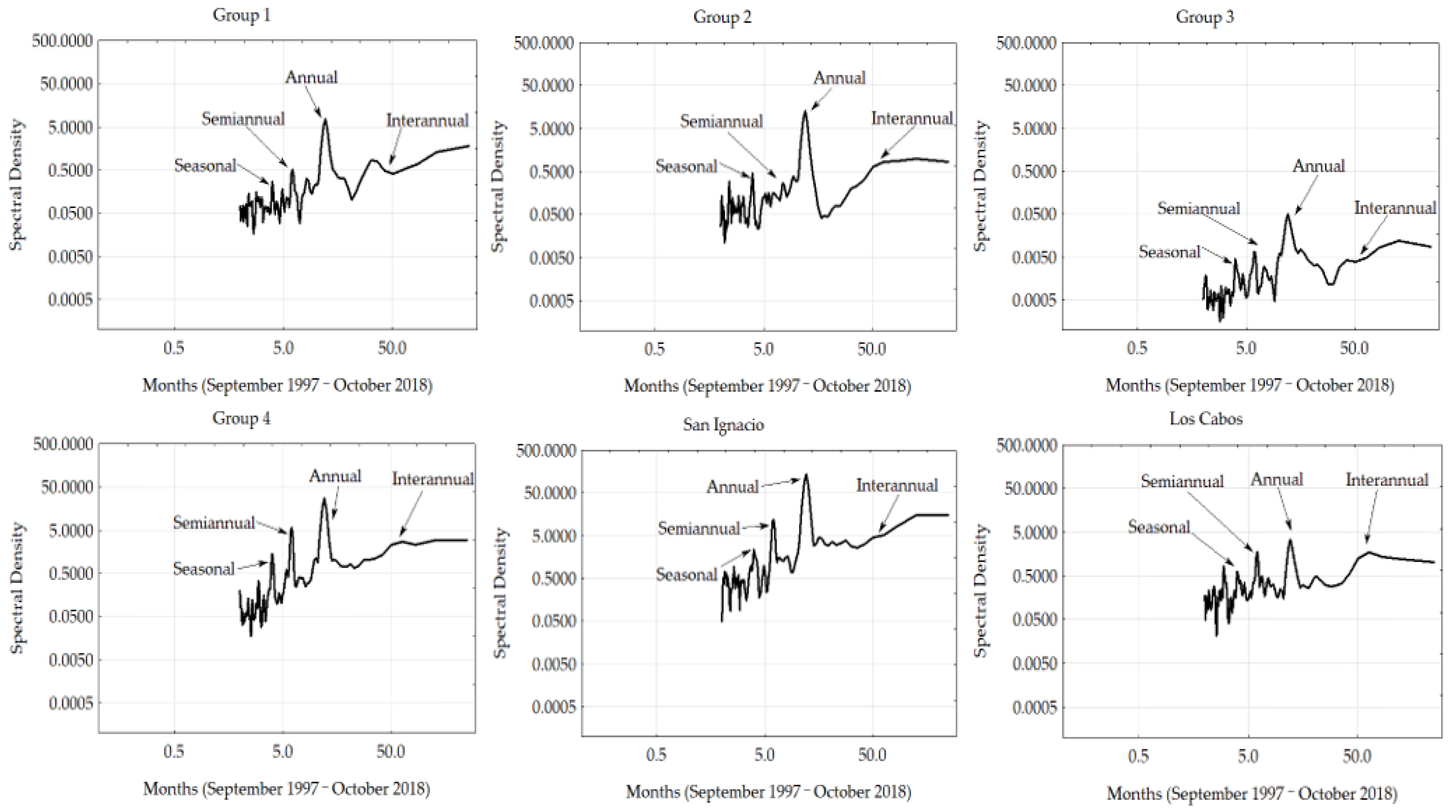
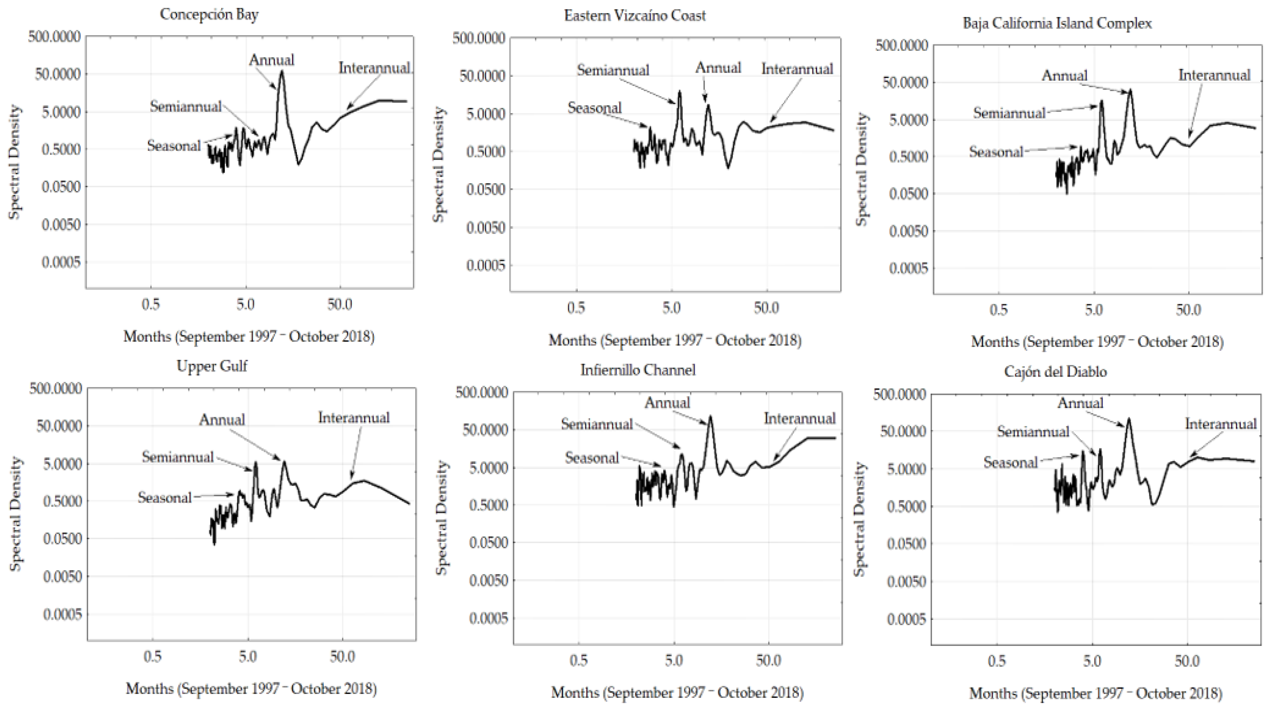
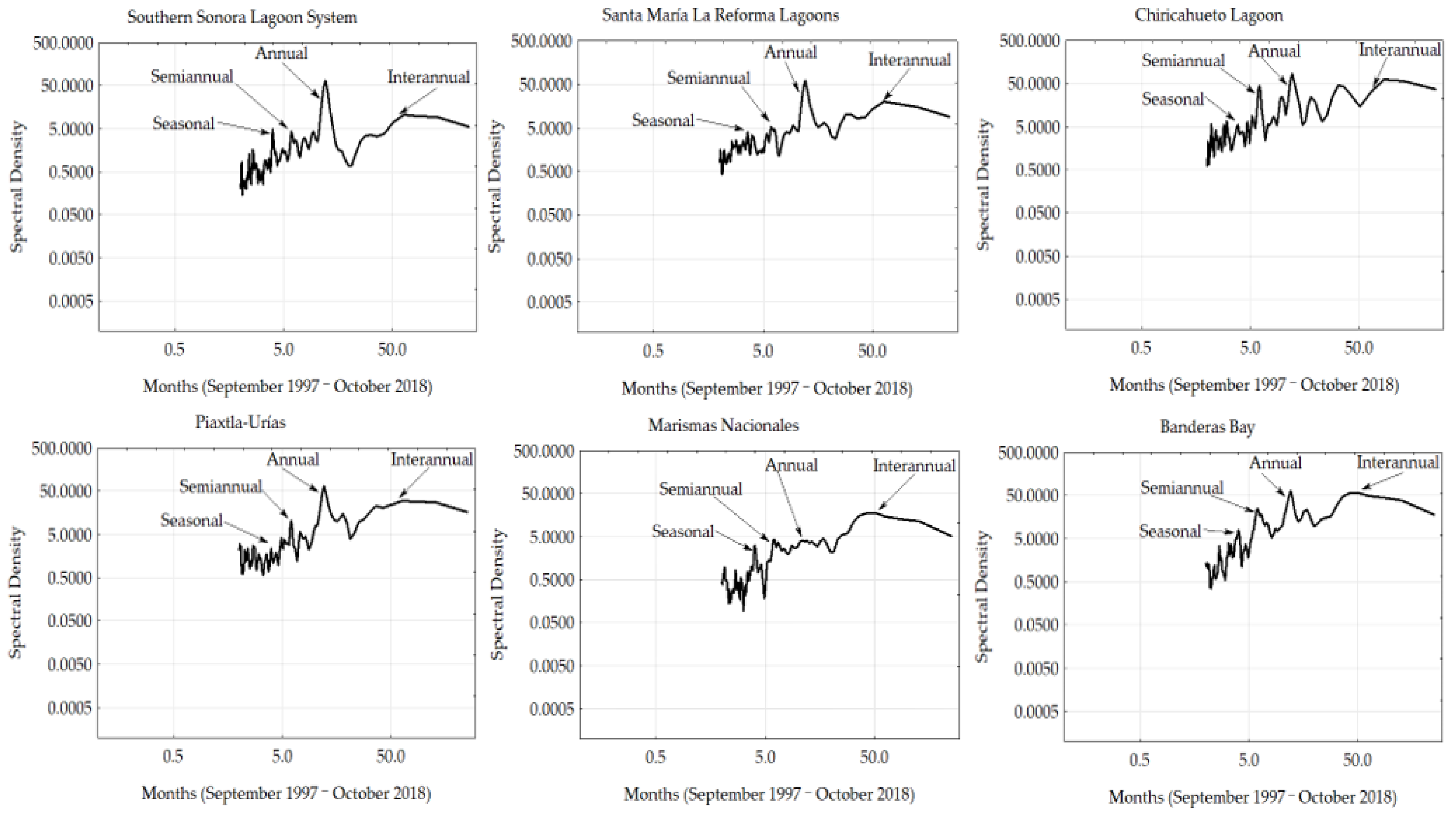
3.3. Fourier Analyses

The Fourier analyses showed a total of four frequencies of variation (Figure 7, Figure 8 and Figure 9). The results indicated that the annual frequency is the most important, followed by the semi-annual one associated with six-month periods—seasonal frequency that determines the 3–4-month periods—and the interannual, whose 3–5-year periods are associated with ENSO climate events. In some of the regions, the semi-annual frequency had a similar spectral density as the annual one, such as the Upper Gulf. Other regions (Concepción Bay, Cajón del Diablo and Southern Sonora Lagoon) obtained equal levels of seasonal spectral density with the semi-annual frequency, whereas the Eastern Vizcaíno Coast showed a higher semi-annual frequency than the annual one. Seasonal frequency was higher than the semi-annual in Group 2. On the other hand, interannual frequency was significant in Marismas Nacionales and Banderas Bay, where this frequency was one of the most important in Chl a variability during the period of study.

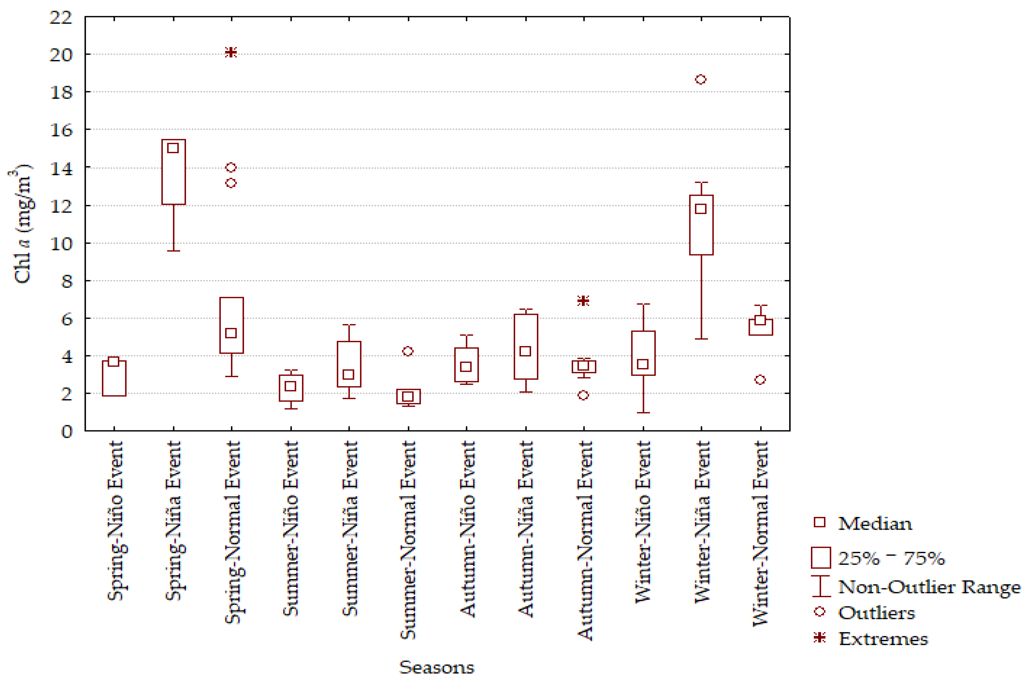
3.4. Statistical Analyses

To determine if significant changes in Chl a concentration occurred, an Elliot-Rothenberg test was performed. In all the regions of the northwest of Mexico, null hypotheses were rejected (p < 0.0001). Seemingly, no trends of changes in Chl a concentration were recorded in these regions.
In addition, for comparison of the monthly Chl a data for all the regions during ENSO and normal conditions, a Pairwise Permutation Test was performed. Monthly Chl a values in all the regions were statistically different (p < 0.05) during all the seasons; most of them were observed during winter and autumn, which were detected by using a Pairwise Permutation Test comparison as a post hoc test. The significant p-values are denoted with letters (Table 2, Table 3, Table 4 and Table 5). When events, into a group or region and for a specific season, share the same letter, no evidence of statistical difference was found.
To illustrate the results shown in Table 2, Table 3, Table 4 and Table 5, box-whisker plots were performed for the monthly Chl a data observed in one region (Piaxtla-Urías), located south of the Gulf of California (Figure 10), showing significant differences in the majority of the seasons of the year (summer, autumn, and winter).

4. Discussion

A total of 18 regions were determined for the whole northwestern region of Mexico through cluster analyses. Four of these regions are located along the South Californian Pacific (Group 1, Group 3, Group 4, and San Ignacio) and the rest of them (14) in the Gulf of California (Group 2, Los Cabos, Concepción Bay, Eastern Vizcaíno Coast, Baja California Complex Island, Upper Gulf, Infiernillo Channel, Cajón del Diablo, Southern Sonora Lagoon System, Santa María La Reforma Lagoons, Chiricahueto Lagoon, Piaxtla-Urías, Marismas Nacionales, and Banderas Bay).
In the case of the South Californian Pacific, diverse similar regionalization studies have been done through short time series analyses to describe Chl a variability and the effect of the interannual events [44,45] as well as for long periods describing Chl a variability and macro and mesoscale phenomena, related to distribution and abundance of sardine stocks [46] besides other studies describing seasonal variability [29]. The resulting number of regions in this marine area can be associated with ocean–atmosphere interaction and effects of the water column physical dynamics that have influence on SST values and nutrient levels in the euphotic zone, changing primary productivity levels of the western coast of the peninsula during spring and summer [47,48] showing variation in the seasonal flow of the California Current System [49]. The physical dynamic influence in Chl a concentration along the western area of the Baja California through geostrophic currents with two large scale cyclonic structures that establish a seasonal variability (summer and autumn) [50,51] in conjunction with strong seasonal winds patterns in spring [52], and consequently, these environmental and oceanographic variabilities generate advection processes showing low temperature water from north to south as well the development of upwelling events in the west coast that increase the nutrient levels [10], of which the effects are significative in the northwestern area of the peninsula; whereas in the south, they occur during spring-summer [49], jointly with the advection of tropical and subtropical waters [53]. In addition, these environmental and oceanographic variabilities have an effect different in the coastal zone due to it being characterized for being areas more dynamic in comparison with the open ocean, developing different Chl a values that can influence the number of regions obtained in the cluster analysis, such as the ones obtained in the South Californian Pacific with a total of three groups (Group 1, Group 3 and Group 3) and an individual region (San Ignacio).
On the other hand, in the Gulf of California, many regionalization proposals have been done based on diverse criteria, such as distribution and abundance of phytoplankton in sediments [54] and satellite-derived images in different periods of study to analyze time series of Chl a concentration [26,31,32,55]. The resulting regions can be associated with atmospheric circulation in conjunction with seasonal winds [37,38,56] that determine circulation patterns in the gulf and influence Chl a concentration. These circulation patterns determine a seasonal variability with a warm period during summer-autumn, which increase SST levels due to an advection process for the direct communication with the Pacific Ocean that allows the entrance of Equatorial Subsurface Water, characterized by being warmer than that of the gulf [56,57] in conjunction with a high solar radiation and evaporation effects causing stratification in the water column, which inhibits the quantity of nutrients along the western zone of the gulf, as well as the presence of southern weak winds that do not have an important effect on the dynamics of the water column [58]. However, winter-spring is the season that corresponds to the cold period, characterized by the development of strong northwestern seasonal wind patterns that generate upwelling events and tidal mixing increasing the phytoplanktonic biomass [31,37,39]. Yet, some of these processes are fairly constant in specific areas of the gulf, generating different phytoplankton concentrations, which explain why the results obtained along the gulf were most of the regions classified as individual ones and only one group was obtained with two regions.
The diverse physical and climatological factors presented in the South Californian Pacific, as well as in the Gulf of California, determine the variability of the Chl a concentration, which is analyzed and considered the aspect of the geographical factors that determine a regionalization process through a cluster analysis based on an oceanographic variable, as is the case of the Chl a concentration, considering a distance of optimal link to establish the regionalization that is taking into account the environmental characteristics and oceanographic aspects of the two marine areas located in northwestern Mexico and thus, be able to describe the environmental variability and oceanographic dynamics in an optimal form.
The descriptive statistical analyses of the time series showed that the lowest Chl a concentrations were observed in Group 3 (0.15 mg/m3) and Los Cabos (0.54 mg/m3). Similar results were reported by Espinosa-Carreón and Valdez-Holguín [59] and Escalante et al. [55], indicating an influence from the Tropical Pacific Ocean through the Inter-Tropical Convergence Zone (ITCZ) movements [60,61]. The ITCZ allows the entrance of oligotrophic and warm waters, which in conjunction with the high solar radiation and evaporation effects [56,57], generates an advection process of tropical waters and, consequently, low Chl a levels in the water column, such as in Los Cabos at the south of the Gulf of California. On the other hand, these low Chl a concentrations can be associated with the fact that regions located in the open sea have systems of oceanic ridges generated by the expansion of oceanic plates, such as R.B. Revillagigedo, from the Group 3 that has a depth of approximately 5000 m [9]; in addition, for being directly influenced by the Eastern Tropical Pacific Ocean, it is considered an area of low phytoplankton productivity due to its clear waters and low concentrations of chlorophyll [62]. Consequently, these regions tend to develop Chl a concentrations below 1 mg/m3 compared to the epipelagic zone and coastal areas where there are physical, climatological, and biological factors that promote higher levels of Chl a. Concerning those regions where the highest Chl a values were observed, they occurred at the Upper Gulf (2.69 mg/m3) in the northern Gulf of California, and particularly the coastal areas of Infiernillo Channel (4.72 mg/m3) and Chiricahueto Lagoon (5.80 mg/m3). Similar results were reported by Millán-Núñez et al. [63] and Ramírez-León [64] in the Upper Gulf, an area with a high concentration of inorganic nutrients, terrigenous types, and total matter in suspension, deriving from tidal mixing and upwelling processes that develop high Chl a concentration [65,66,67]. In the case of the Infiernillo Channel coastal zone, high Chl a values were reported by García-Morales et al. [33] and Robles-Tamayo et al. [68], indicating that these results are associated with tidal mixing and upwelling processes, which derive from intense seasonal wind patterns in the Gulf of California [69,70], particularly in the region of the Infiernillo Channel, considered a shallow area that develops a constant well-mixed water column [71]. Another factor that can explain these high Chl a concentrations in coastal regions of the gulf, such as the Chiricahueto Lagoon, is shrimp farmland runoff, particularly south of the state of Sonora and north of Sinaloa, raising inorganic nutrient levels, such as nitrogen, phosphorous, and iron [72,73], and modifying phytoplankton community composition and ecosystems of the coastal zone of the gulf [74]. Similar effects were reported by Miranda et al. [75] in southern Sonora that are also related to shrimp farm runoffs increasing nitrogen and phosphorous levels, thus influencing a nutrient increase in ecosystems in the coastal zone of the gulf. Additionally, Martínez-López et al. [76] reported high Chl a concentration (15 mg/m3) in northern Sinaloa, associated with farmland runoffs as well as wastewater effluents and seasonal rains that influence variability of phytoplankton and cyanobacteria.
The analyses of Chl a concentration anomalies in the regions from the South Californian Pacific and the Gulf of California showed negative and positive anomalies associated with ENSO interannual events. In general, the effect of anomalies in Chl a levels in each one of the areas are observed in the following periods: July 1998–February 2001, November 2005–March 2006, June 2007–March 2009, and June 2010–April 2012 during La Niña event; positive anomalies were generated, increasing the Chl a concentration while the periods of September 1997–September 1998, June 2002–February 2003, July 2004–February 2005, September 2006–January 2007, July 2009–March 2010, and October 2014–April 2016 influenced by the El Niño event developed negative anomalies, decreasing Chl a values. These effects of interannual variability have been reported by different authors [77,78,79,80] in the South Californian Pacific, which were associated with the direct influence of the cold water of the California Current Systems that developed upwelling processes of subsurface water. These upwelling processes have a significant effect on Chl a variability along the area [77], as well as poleward advection of subtropical water [53] and the North Pacific Decadal Oscillation phase [79]. Some other research works [81,82] have reported the presence of anomalous subarctic water along the west area of the state of Baja California, influencing interannual variation in deep waters, and determining the intensity of these interannual events.
The effects of interannual events were also observed in the regions from the Gulf of California. Similar results to the ones reported were obtained by other authors [55,68,83], where hydrographic characteristics are influenced by the direct communication with the Tropical Pacific Ocean that enables the entrance of equatorial surface water [57]. These regions are characterized by being warmer and more oligotrophic than the water of the gulf, which also has the effects of the El Niño event. Chl a concentration decreases from north to south, which is more significant in the southern gulf because of its direct communication with the Pacific Ocean, such as the regions of Marismas Nacionales, Banderas Bay, and the Gulf Entrance. However, the El Niño event has a minor effect within the gulf, particularly in the regions of Midriff Islands and the Ballenas Channel [69,70,84], due to the different circulation patterns when compared to other gulf areas that develop constant tidal mixing and upwelling processes. A similar effect was reported in the Upper Gulf [65,66] where phytoplankton biomass response was low due to these interannual events and their oceanographic conditions that derive from wind patterns. Nevertheless, other research works [85] reported a disruption in wind patterns due to the effect of ENSO events, modifying upwelling processes, which was more significant during strong warm ENSO, influenced by wind intensity and increased SST levels [83]. This effect was mainly observed in most of the Chl a time series anomalies, during strong El Niño events (1997–1998, 2002–2003, 2009–2010 and 2014–2016).
In addition, the effects of the El Niño (1997–1998; 2009–2010 and 2015–2016) and La Niña (1998–1999; 1999–2000 and 2000–2001, 2007–2008) events had important effects on Chl a variability along the period of study, decreasing and increasing the levels during these interannual events and having a delayed response from 2010 to 2018. A similar effect was reported by Robles-Tamayo et al. [68] in the eastern coastal zone of the Gulf of California; the authors detected a delayed response during the periods of 2009–2010 and 2015–2016, which continued until the final period of this study, associated with moderate and very strong El Niño events [86]. All the occurring factors in the South Californian Pacific and Gulf of California explain the results that some regions are more responsive to SOI variability, mainly those south of the Gulf of California that have a direct communication with the Pacific Ocean, as well as the significant statistical differences observed in Chl a concentration during interannual events and normal conditions for all the seasons of the year.
For all the regions, the main variability frequency for Chl a concentration was the annual one, which was also reported by Ortíz-Ahumada et al. [79] on the southern California Current System and by García-Morales et al. [33] in the central coastal zone of the Gulf of California. Ortíz-Ahumada et al. [79] indicated that the annual Chl a cycle is associated with the dynamics of the California Current System that determines Chl a variability throughout the year with high levels from February to July and minimum ones from August to December. A similar result was previously reported by Espinosa-Carreón et al. [87] along the western region of Baja California in the California Current System. They obtained maximum values of Chl a during spring, mainly in inshore areas, causing phytoplankton biomass growth derived from upwelling processes and wind patterns that determine the annual signal of Chl a during the year. In the case of the Gulf of California, García-Morales et al. [33] explained that annual frequency derives from the ocean–atmosphere interaction that occurs along the year, determining seasonal wind patterns, which play an important role in upwelling events of the gulf, in conjunction with mesoscale phenomena (cyclonic and anticyclonic gyres). These interactions are present in the current systems from the Mexican Coastal Zone, modulated by the movements of the ITCZ, determining oceanographic conditions of the marine and coastal ecosystems, such as Chl a concentration. López-Calderón et al. [88] analyzed mesoscale variability in the Pacific Ocean; the authors observed that Chl a variability is also associated with the development of cyclonic and anticyclonic gyres during winter and spring, causing an increase in Chl a levels. The semi-annual frequency is the one that occurs every six months and is characterized by developing specific circulation patterns of the water column, reported by different authors [66,70], and we concluded that the frequency of variation is mainly determined by upwelling effects and mesoscale processes that develop these changes every six months in Chl a variability. Herrera-Cervantes [89] analyzed the main frequencies of variation at La Paz Bay and observed that the semi-annual frequency of variation plays an important role in Chl a variability, determining 31% of the Chl a concentration, reaching high levels around 1.5 mg/m3 along the coast. The author concludes that Chl a variability is mainly associated with upwelling events and coastal currents determined by seasonal wind patterns. Seasonal frequency is associated with changes occurring every three or four months and can be associated to gyre circulation patterns in the water column [61], which have an effect during water exchange, such as in the eastern coast of the Gulf of California [56,90]. This frequency of variation influences upwelling effects during different seasons throughout the year with an increase in phytoplankton biomass, which was observed in Group 2 and in coastal regions of the gulf.
Interannual frequency varies from three to five years and is associated to the warm (El Niño) and cold (La Niña) events. This interannual variability has been reported in the South Californian Pacific [78,80] and Gulf of California [55,59] due to advection of subtropical water effects of the North Pacific Decadal Oscillation and the presence of anomalous waters, such as subarctic ones [77,79,82]. According to the spectral analysis of the regions in this study, interannual frequency was greater in the areas of the state of Nayarit (Marismas Nacionales and Banderas Bay), which is south of the gulf. This area has a wide and direct communication with the Tropical Pacific Ocean, in comparison with the other regions of northwestern Mexico, which has the effect of warmer waters compared with the gulf, and declining nutrient and, consequently, Chl a levels. Cepeda-Morales et al. [91] also reported this interannual variability at the continental shelf in front of Nayarit; the authors analyzed Chl a temporal variations and observed clear interannual events with a variation from 0.7 to 11.5 mg/m3, attributed to ENSO events. Moreover, it is important to consider that diverse human activities may have the capacity to modify the Earth ecological systems and large-scale components, developing “tipping points”, that is, a variation of phenomena that generate alterations in the Earth’s climate systems [92]. An example of climate variation is the ENSO event, where the gradual anthropogenic influence modifies its intensity levels through an increase in ocean heat. This variation causes deepening in the thermocline in the East Equatorial Pacific and, consequently, a high variability in the amplitude and frequency of El Niño [93] and La Niña events, causing an increase in easterly winds and developing more of an upwelling process in the water column [94]. This interannual variability is observed in south of the regions of Northwest Mexico, mainly in those located south of the Gulf of California (Marismas Nacionales and Banderas Bay), where the Fourier analysis showed a significant influence in interannual variability of Chl a levels throughout the period of study. This situation is due to the ITCZ system movements that allow the entrance of warmer waters to the southern area of the Gulf of California and are characterized with low nutrient levels, affecting Chl a variability when compared with the central and northern areas of the gulf where ENSO variability has a different effect due to the physical dynamics along the area that influence Chl a levels.
According to the results previously discussed regarding Chl a variability, the analyses show that it is influenced by diverse climatological and physical processes, observed in different spatiotemporal scales. Therefore, its variation can have an effect on the structure and function of marine and coastal ecosystems due to possible changes in distribution and abundance of the marine resources. This effect was also reported by García-Morales et al. [33] and García-Morales et al. [34], concluding that Chl a variation can affect the number of species in the marine ecosystems.
Howrever, despite chlorophyll a concentration variability caused by the processes previously mentioned, as well as the interannual phenomena (ENSO events), the South Californian Pacific and Gulf of California have shown a resilience capacity to these adverse condition effects along the period of study, mainly where SOI Index and time series showed an important correlation in the first year of the period of study, whereas after the period 2009–2010, a delay in Chl a increase and a lag with SOI Index were observed. Nevertheless, the statistical analysis showed no significant trend of change in Chl a concentration for all the regions, indicating a maintenance of the normal environment in the ecosystem, thus, supporting a large diversity of species. This effect was reported by Escalante et al. [55] in the Gulf of California where a delayed response of about three to six months was observed, re-establishing normal conditions in Chl a levels after the effects of interannual events. This study showed that in time series analyses and time series anomalies, high and low chlorophyll concentrations returned to normal conditions during the period of study.
Different studies of environmental variability and oceanographic dynamics have been performed in northwestern Mexico through the analysis of Chl a to describe its influence on the marine ecosystems and their natural resources. An important one is from Sandoval-Lugo et al. [95], who analyzed the movement of loggerhead sea turtles (Caretta caretta) in the Gulf of California through satellite tracking and SST and Chl a data to determine their movements and habitats, determining that this species is distributed in waters from 10 to 80 m in depth with eutrophic levels, showing a mean Chl a concentration that varies from 0.28 to 13.14 mg/m3. Another research work corresponds to Silveyra-Bustamante et al. [96] at Cabo Pulmo National Park, in the Gulf of California. They described seasonal variability of gelatinous zooplankton, concluding that the abundance of gelatinous zooplankton had a positive association with sea surface chlorophyll a concentration, and also with the direction and velocity of wind patterns; both of these influenced its abundance in October, indicating that mesotrophic conditions sustain high biomass and diversity of the zooplankton in Cabo Pulmo. The research results in this study showed that the analysis of Chl a concentration and its variability are fundamental to study environmental variability and oceanographic dynamics, which are necessary to describe diverse physical, climatological, and biological aspects of the marine and coastal ecosystems, such as distribution and abundance of their marine resources. An appropriate analysis of Chl a concentrations allows for the developing of suitable ecological characterization to be able to determine possible trends of change associated with environmental and oceanographic factors.

5. Conclusions

The variability of the Chl a concentration variability of the Chl a concentration from the South Californian Pacific and Gulf of California derive from geographic location effects that show a direct interaction with the Pacific Ocean, determining environmental and oceanographic conditions and different Chl a concentration at different spatiotemporal scales, from seasonal to interanual, as well as to the climate variability associated with climate change, which generates diverse physical, climatological, and biological processes. The analysis of Chl a concentration allowed us to perform an optimal characterization of different regions in the South Californian Pacific and Gulf of California through a cluster analysis defining a total of 18 regions, based on the Chl a concentration and considering the grouped regions with similar oceanographic and environmental characteristics with an adequate linkage distance, which showed an annual variation with higher Chl a levels in coastal zones than the oceanic ones.
Evidence was found for rejecting the non-stationary assumption in each one of the time series despite the effects of different interannual events as El Niño (1997–1998, 2004–2005, 2010 and 2014–2016) and La Niña (1999–2001, 2007–2009 and 2011–2013) that caused a change in Chl a concentration and a delay with the Southern Oscillation Index, showing a resilience capacity in the analyzed PMR. In addition, statistical evidence against the assumption of no seasonal differences in Chl a concentration was observed between the interannual (El Niño and La Niña) events and normal conditions in many regions. The Fourier analysis determined four frequencies of variation that influence Chl a concentration variability at different temporal scales, of which the annual frequency is the main one in all the regions.
To conclude, based on the results obtained from this study, the analysis of the Chl a concentration, as well its constant monitoring and the regionalization process using this variable, show evidence of its importance in obtaining updated oceanographic and environmental information of different areas; therefore, this allows us to study different climatological and biological processes that can impact the abundance and distribution of marine organisms and natural resources, as well in the functioning of marine and coastal ecosystems. The information obtained will be also very useful to generate an adequate conservation and research management of the biodiversity and develop recommendations on the future environmental activity allowed or required for these regions.

Author Contributions

Conceptualization, J.R.R.-L. and R.G.-M.; methodology, C.M.R.-T., J.R.R.-L., R.G.-M., G.F.-P., M.C.P.-G. and L.F.E.-O.; software, J.R.R.-L., R.G.-M. and G.F.-P.; validation, C.M.R.-T., J.R.R.-L., R.G.-M., G.F.-P., M.C.P.-G. and L.F.E.-O.; formal analysis, G.F.-P.; investigation, C.M.R.-T., J.R.R.-L., R.G.-M., G.F.-P., M.C.P.-G. and L.F.E.-O.; resources, J.R.R.-L. and R.G.-M.; data curation, C.M.R.-T.; writing—original draft preparation, C.M.R.-T.; writing—review and editing, C.M.R.-T., J.R.R.-L., R.G.-M., G.F.-P., M.C.P.-G. and L.F.E.-O.; visualization, C.M.R.-T., J.R.R.-L., R.G.-M., G.F.-P., M.C.P.-G. and L.F.E.-O.; supervision, C.M.R.-T., J.R.R.-L., R.G.-M., G.F.-P., M.C.P.-G. and L.F.E.-O.; project administration, J.R.R.-L. and R.G.-M.; funding acquisition, J.R.R.-L. and R.G.-M. All authors have read and agreed to the published version of the manuscript.

Funding

This research was funded by Consejo Nacional de Ciencia y Tecnología (Spanish for National Council of Science and Technology; abbreviated CONACYT) project: (A3-S-77965). Project “Cambios Históricos y Recientes en la Distribución de Especies Bentónicas y Demersales Marinas del del Golfo de California como Efecto del Calentamiento Global. Detección de especies con potencial invasivo”.

Acknowledgments

This research was financed by CONACYT project: (A3-S-77965). The authors acknowledge to the Program in Biosciences, Division of Biological Health Sciences of the University of Sonora. Diana Fischer for English edition. Carlos Manuel Robles-Tamayo is a CONACYT fellow.

Conflicts of Interest

The authors declare no conflict of interest.

References

  1. Lara-Lara, J.R.; Arenas-Fuentes, V.; Bazán-Guzmán, C.; Díaz-Castañeda, V.; Escobar-Briones, E.; García-Abad, M.; Espe-jel-Carvajal, M.I.; Guzmán-Arroyo, M.; Ladah, L.B.; López-Hernández, M.; et al. Los Ecosistemas Marinos. In Capital Natural de México. Vol. I: Conocimiento Actual de la Biodiversidad, 1st ed.; Soberón, J., Halffter, G., y Llorente, J., Eds.; Comisión Nacional para el Conoci-miento y Uso de la Biodiversidad, CONABIO: Ciudad de México, México, 2008; Volume 1, pp. 135–159. [Google Scholar]
  2. Rosales-Nanduca, H.; Gerrodette, T.; Urbán-R, J.; Cárdenas-Hinojosa, G.; Medrano-González, L. Macroecology of marine mammal species in the Mexican Pacific Ocean: Diversity and distribution. Mar. Ecol. Prog. Ser. 2011, 431, 281–291. [Google Scholar] [CrossRef]
  3. Saldaña-Ruiz, L.E.; García-Rodríguez, E.; Pérez-Jiménez, J.; Tovar-Ávila, J.; Rivera-Téllez, E. Chapter Two—Biodiversity and Conservation of Sharks in Pacific Mexico. In Advances in Marine Biology, 1st ed.; Larson, S.E., Lowry, D., Eds.; The University of Warwick: Coventry, UK, 2019; Volume 83, pp. 11–60. [Google Scholar]
  4. Lluch-Cota, S.E.; Aragón-Noriega, E.A.; Arreguín-Sánchez, F.; Aurioles-Gamboa, D.; Bautista-Romero, J.J.; Brusca, R.C.; Cervantes-Duarte, R.; Cortés-Altamirano, R.; Del-Monte-Luna, P.; Esquivel-Herrera, A.; et al. The Gulf of California: Review of ecosystems status and sustainability challenges. Pro. Oce. 2007, 73, 1–26. [Google Scholar] [CrossRef]
  5. Arreguín-Sánchez, F.; del Monte-Luna, P.; Zetina-Rejón, M.J.; Albáñez-Lucero, M.O. The Gulf of California Large Marine Ecosystem: Fisheries and other natural resources. Environ. Dev. 2017, 22, 71–77. [Google Scholar] [CrossRef]
  6. Espinosa, H. El Pacífico Mexicano. Ciencias 2004, 76, 14–21. [Google Scholar]
  7. Lluch-Cota, S.E.; Parés-Sierra, A.; Magaña-Rueda, V.O.; Arreguín-Sánchez, F.; Bazzino, G.; Herrera-Cervantes, H.; Lluch-Belda, D. Changing climate in the Gulf of California. Prog. Oceanogr. 2010, 87, 114–126. [Google Scholar] [CrossRef]
  8. Arriaga-Cabrera, L.; Aguilar, A.; Espinoza, J.M. Regiones Marinas y Planeación Para la Conservación de la Biodiversidad. In Capital Natural de México. Vol. II: Estado de Conservación y Tendencias de Cambio, 1st ed.; Dirzo, R., González, R., March, I.J., Eds.; Comisión Nacional para el Conocimiento y Uso de la Biodiversidad, CONABIO: Ciudad de México, México, 2009; Volume 2, pp. 433–457. [Google Scholar]
  9. Wilkinson, T.A.C.; Wilken, E.; Bezaury-Creel, J.; Hourigan, T.F.; Agardy, T.; Herrmann, H.; Janishevski, L.; Madden, C.; Morgan, L.; Padilla, M. Ecorregiones Marinas de América del Norte; Comisión para la Cooperación Ambiental: Montreal, QC, Canada, 2009; pp. 107–108. [Google Scholar]
  10. Gaxiola-Castro, G.; Cepeda-Morales, J.C.A.; Nájera-Martínez, S.; Espinosa-Carreón, T.L.; De la Cruz-Orozco, M.E.; So-sa-Avalos, R.; Aguirre-Hernández, E.; Cantú-Ontiveros, J.P. Biomasa y Producción de Fitoplancton. In Dinámica del Ecosistema Pelágico Frente a Baja California, 1997–2007. In Diez Años de Investigaciones Mexicanas de la Corriente de California, 1st ed.; Gaxiola-Castro, G., Durazo-Arvizu, R., Eds.; Secretaría del Medio Ambiente y Recursos Naturales, Instituto Nacional de Ecología, Centro de Investigación Científica y de Educación Superior de Ensenada, Universidad Autónoma de Baja California: Ensenada, México, 2010; pp. 59–85. [Google Scholar]
  11. Valiela, I. Marine Ecological Processes, 2nd ed.; Springer: New York, NY, USA, 1995; p. 645. [Google Scholar]
  12. Ramírez, D.G.; Giraldo, A.; Tovar, J. Primary production, biomass, and taxonomic composition of coastal and oceanic phy-toplankton in the Colombian Pacific (September–October 2004). Lat. Ame. Aqua. Res. 2006, 34, 211–216. [Google Scholar]
  13. Morales-Hernández, J.C.; Carrillo-González, F.M.; Farfán-Molina, L.M.; Cornejo-López, V.M. Vegetation change cover in the coastal region of Bahia de Banderas. Mexico. Cal. 2016, 38, 17–29. [Google Scholar]
  14. Rohli, R.V.; Vega, A. Climatology, 4th ed.; Jones & Bartlett Learning: Burlington, MA, USA, 2018; p. 60. [Google Scholar]
  15. Soto-Mardones, L.; Marinone, S.; Parés-Sierra, A. Time and spatial variability of sea surface temperature in the Gulf of California. Cienc. Mar. 1999, 25, 1–30. [Google Scholar] [CrossRef]
  16. Henson, S.A.; Sarmiento, J.L.; Dunne, J.P.; Bopp, L.; Lima, I.; Doney, S.C.; John, J.; Beaulieu, C. Detection of anthropogenic climate change in satellite records of ocean chlorophyll and productivity. Biogeosciences 2010, 7, 621–640. [Google Scholar] [CrossRef]
  17. Gregg, W.W.; Rousseaux, C.S. Decadal trends in global pelagic ocean chlorophyll: A new assessment integrating multiple satellites, in situ data, and models. J. Geophys. Res. Oceans 2014, 119, 5921–5933. [Google Scholar] [CrossRef]
  18. Nayak, R.K.; Mishra, S.K.; Satyesh, G.; Nagamani, P.V.; Choudhury, S.B.; Seshasai, M.V.R. Remote sensing application in satellite oceanography. Ind. Geo. J. 2018, 93, 156–165. [Google Scholar]
  19. Longhurst, A.R. Ecological Geography of the Sea, 2nd ed.; Elsevier Academic Press: San Diego, CA, USA, 2007; p. 5. [Google Scholar]
  20. Devi, G.K.; Ganasri, B.; Dwarakish, G. Applications of Remote Sensing in Satellite Oceanography: A Review. Aquat. Procedia 2015, 4, 579–584. [Google Scholar] [CrossRef]
  21. Gregg, W.W.; Conkright, M.E. Global seasonal climatologies of ocean chlorophyll: Blending in situ and satellite data for the Coastal Zone Color Scanner era. J. Geophys. Res. Oceans. 2001, 106, 2499–2515. [Google Scholar] [CrossRef]
  22. Dutkiewicz, S.; Hickman, A.E.; Jahn, O.; Henson, S.; Beaulieu, C.; Monier, E. Ocean Color Signature of Climate Change. Nat. Com. 2019, 10, 1–13. [Google Scholar]
  23. Krug, L.A.; Platt, T.; Sathyendranath, S.; Barbosa, A.B. Ocean surface partitioning strategies using ocean colour remote Sensing: A review. Prog. Oceanogr. 2017, 155, 41–53. [Google Scholar] [CrossRef]
  24. Schwarz, J.N. Dynamic partitioning of tropical Indian Ocean surface waters using ocean colour data—Management and modelling applications. J. Environ. Manag. 2020, 276, 111308. [Google Scholar] [CrossRef]
  25. Krug, L.A.; Platt, T.; Sathyendranath, S.; Barbosa, A.B. Patterns and drivers of phytoplankton phenology off SW Iberia: A phenoregion based perspective. Prog. Oceanogr. 2018, 165, 233–256. [Google Scholar] [CrossRef]
  26. Heras-Sánchez, M.C.; Valdez-Holguín, J.E.; Garatuza-Payán, J.; Cisneros-Mata, M.A.; Díaz-Tenorio, L.M.; Robles-Morua, A.; Ha-zas-Izquierdo, R.G. Regiones del Golfo de California determinadas por la distribución de temperatura superficial del mar y la clorofila-a. Biotecnia 2019, 21, 13–21. [Google Scholar] [CrossRef]
  27. Santamaría-del-Angel, E.; González-Silvera, A.; Millán-Núñez, R.; Callejas-Jiménez, M.E.; Cajal-Medrano, R. Determining Dynamic Biogeographic Regions Using Remote Sensing Data. In Handbook of Satellite Remote Sensing Image Interpretation: Applications for Marine Living Resources Conservation and Management, 1st ed.; Morales, J., Stuart, V., Platt, T., Sathyendranath, S., Eds.; EU PRESPO and IOCCG: Dartmouth, NS, Canada, 2011; Volume 1, pp. 273–293. [Google Scholar]
  28. Millán-Núñez, R.; Alvarez-Borrego, S.; Trees, C.C. Modeling the vertical distribution of chlorophyll in the California Current System. J. Geo. Res. 1997, 102, 8587–8595. [Google Scholar] [CrossRef]
  29. Thomas, A.C.; Mendelssohn, R.; Weatherbee, R. Background trends in California Current surface chlorophyll concentrations: A state-space view. J. Geophys. Res. Oceans 2013, 118, 5296–5311. [Google Scholar] [CrossRef]
  30. Hernández-de la Torre, B.; Aguirre-Gómez, R.; Gaxiola-Castro, G.; Álvarez-Borrego, S.; Gallegos-García, A.; Rosete-Vergés, F.; Bocco-Verdinelli, G. Ordenamiento Ecológico Marino en el Pacífico Norte mexicano: Propuesta metodológica. Hidrobiológica 2015, 25, 151–163. [Google Scholar]
  31. Santamaría-Del-Angel, E.; Alvarez-Borrego, S.; Muller-Karger, F.E. Gulf of California biogeographic regions based on coastal zone color scanner imagery. J. Geophys. Res. Earth Surf. 1994, 99, 7411–7421. [Google Scholar] [CrossRef]
  32. Kahru, M.; Marinone, S.; Lluch-Cota, S.; Parés-Sierra, A.; Mitchell, B.G. Ocean-color variability in the Gulf of California: Scales from days to ENSO. Deep-Sea Res. II 2004, 51, 139–146. [Google Scholar] [CrossRef]
  33. García-Morales, R.; López-Martínez, J.; Valdez-Holguin, J.E.; Herrera-Cervantes, H.; Espinosa-Chaurand, L.D. Environmental Variability and Oceanographic Dynamics of the Central and Southern Coastal Zone of Sonora in the Gulf of California. Remote Sens. 2017, 9, 925. [Google Scholar] [CrossRef]
  34. García-Morales, R.; Pérez-Lezama, E.L.; Shirasago-Germán, B. Influence of environmental variability of baleen whales (suborden mysticeti) in the Gulf of California. Mar. Eco. 2017, 38, 10. [Google Scholar]
  35. Gaxiola-Castro, G.; Durazo, R. Introducción. In Dinámica del Ecosistema Pelágico Frente a Baja California, 1997–2007. Diez años de Investigaciones Mexicanas de la Corriente de California, 1st ed.; Gaxiola-Castro, G., Durazo-Arvizu, R., Eds.; Secretaría del Medio Ambiente y Recursos Naturales, Instituto Nacional de Ecología, Centro de Investigación Científica y de Educación Superior de Ensenada, Universidad Autónoma de Baja California: Ensenada, México, 2010; pp. 13–24. [Google Scholar]
  36. Espinosa-Carreón, T.L.; Gaxiola-Castro, G.; Beier, E.; Strub, P.T.; Kurczyn, J.A. Effects of mesoscale processes on phytoplankton chlorophyll off Baja California. J. Geo. Res. Oce. 2012, 117, C04005. [Google Scholar] [CrossRef]
  37. Alvarez-Borrego, S. Physical, Chemical and Biological Oceanography of the Gulf of California. In The Gulf of California: Biodiversity and Conservation, 2nd ed.; Brusca, R., Ed.; The University of Arizona Press: Tucson, AZ, USA, 2010; pp. 24–48. [Google Scholar]
  38. Alvarez-Borrego, S.; Lara-Lara, J.R. The Physical Environment and Primary Productivity of the Gulf of California. In The Gulf of California, Province of the Californias, 1st ed.; Dauphin, J.P., Simoneit, B.R.T., Eds.; American Association of Petroleum Geologist: Tulsa, OK, USA, 1991; pp. 555–567. [Google Scholar]
  39. Alvarez-Borrego, S. Phytoplankton biomass and production in the Gulf of California: A review. Bot. Mar. 2012, 55, 119–128. [Google Scholar] [CrossRef]
  40. Kahru, M. The California Current Merged Satellite-Derived 4-km Dataset. 2020. Available online: http://www.wimsoft.com/CC4km.htm (accessed on 29 September 2020).
  41. Kahru, M.; Kudela, R.M.; Manzano-Sarabia, M.; Mitchell, B.G. Trends in the surface chlorophyll of the California Current: Merging data from multiple ocean color satellites. Deep Sea Res. Part II Top. Stud. Oceanogr. 2012, 77–80, 89–98. [Google Scholar] [CrossRef]
  42. Kahru, M. Windows Image Manager, WIM Software (Ver. 9.06) and User’s Manual. 2016. Available online: http://www.wimsoft.com/ (accessed on 29 September 2020).
  43. Everitt, B.S.; Landau, S.; Leese, M.; Stahl, D. Cluster Analysis, 5th ed.; John Wiley & Sons Ltd.: Chichester, UK, 2011; p. 13. [Google Scholar]
  44. Kahru, M.; Mitchell, G. Influence of the 1997–1998 El Niño on surface chlorophyll in the California Current. Geo. Res. Let. 2000, 27, 2937–2940. [Google Scholar] [CrossRef]
  45. Kahru, M.; Mitchell, G. Seasonal and nonseasonal variability of satellite-derived chlorophyll and colored dissolved organic matter concentration in the California Current. J. Geo. Res. 2001, 102, 2517–2529. [Google Scholar] [CrossRef]
  46. García-Morales, R. Variabilidad Oceanográfica del Hábitat de Los Stocks de Sardinops Sagax (Jenyns, 1842) (Clupeiformes: Clupeidae) en el Sistema de Corriente de California (1981–2005). Ph.D. Thesis, Centro Interdisciplinario de Ciencias Mari-nas-Instituto Politécnico Nacional, La Paz, Baja California Sur, México, 2012. [Google Scholar]
  47. Zaitsev, O.; Cervantes-Duarte, R.; Montante, O.; Gallegos-Garcia, A. Coastal Upwelling Activity on the Pacific Shelf of the Baja California Peninsula. J. Oceanogr. 2003, 59, 489–502. [Google Scholar] [CrossRef]
  48. Pérez-Brunius, P.; López, M.; Páres-Sierra, A.; Pineda, J. Comparison of upwelling indices off Baja California derived from three different wind data sources. CalCOFI Rep. 2007, 48, 204–212. [Google Scholar]
  49. Durazo, R.; Ramírez-Manguilar, A.M.; Miranda, L.E.; Soto-Mardones, L.A. Climatología de variables oceanográficas. In Di-námica del Ecosistema Pelágico Frente a Baja California, 1997–2007. Diez años de Investigaciones Mexicanas de la Corriente de California, 1st ed.; Gaxiola-Castro, G., Durazo-Arvizu, R., Eds.; Secretaría del Medio Ambiente y Recursos Naturales, Instituto Nacional de Ecología, Centro de Investigación Científica y de Educación Superior de Ensenada, Universidad Autónoma de Baja California: Ensenada, México, 2010; pp. 25–57. [Google Scholar]
  50. Durazo, R. Climate and upper ocean variability off Baja California, Mexico: 1997–2008. Prog. Oceanogr. 2009, 83, 361–368. [Google Scholar] [CrossRef]
  51. Durazo, R. Seasonality of the transitional region of the California Current System off Baja California. J. Geophys. Res. Oceans 2015, 120, 1173–1196. [Google Scholar] [CrossRef]
  52. Castro, R.; Martínez, J.A. Variabilidad espacial y temporal del campo del viento. In Dinámica del Ecosistema Pelágico Frente a Baja California, 1997–2007. Diez Años de Investigaciones Mexicanas de la Corriente de California, 1st ed.; Gaxiola-Castro, G., Durazo-Arvizu, R., Eds.; Secretaría del Medio Ambiente y Recursos Naturales, Instituto Nacional de Ecología, Centro de Investigación Científica y de Educación Superior de Ensenada, Universidad Autónoma de Baja California: Ensenada, México, 2010; pp. 129–147. [Google Scholar]
  53. Durazo, R.; Baumgartner, T. Evolution of oceanographic conditions off Baja California: 1997–1999. Prog. Oceanogr. 2002, 54, 7–31. [Google Scholar] [CrossRef]
  54. Round, F. The Gulf of California. Part I. Its composition, distribution and contribution to the sediments. J. Exp. Mar. Biol. Ecol. 1967, 1, 76–97. [Google Scholar] [CrossRef]
  55. Escalante, F.; Valdez-Holguín, J.E.; Álvarez-Borrego, S.; Lara-Lara, J.R. Temporal and spatial variation of sea surface temperature, chlorophyll a, and primary productivity in the Gulf of California. Cie. Mar. 2013, 39, 203–215. [Google Scholar] [CrossRef]
  56. Alvarez-Borrego, S. Gulf of California. In Ecosystems of the World, 26: Estuaries and Enclosed Seas, 1st ed.; Ketchum, B.H., Ed.; Elsevier Scientific: New York, NY, USA, 1983; pp. 427–429. [Google Scholar]
  57. Torres-Orozco, E. Análisis Volumétrico de las Masas de Agua del Golfo de California. Master’s Thesis, Centro de Investigación Científica y de Educación Superior de Ensenada, Ensenada, Baja California, México, 1993. [Google Scholar]
  58. Santamaría-del-Angel, E.; Álvarez-Borrego, S.; Millán-Núñez, R.; Muller-Karger, F.E. Sobre el efecto de las surgencias de verano en la biomasa fitoplanctónica del Golfo de California. Rev. Soc. Mex. Hist. Nat. 1999, 49, 207–212. [Google Scholar]
  59. Espinosa-Carreón, T.L.; Valdez-Holguín, J.E. Variabilidad interanual de clorofila en el Golfo de California. Eco. Apl. 2007, 6, 83–92. [Google Scholar] [CrossRef] [Green Version]
  60. Lavín, M.F.; Beier, E.; Badan, A. Estructura hidrográfica y circulación del Golfo de California: Escalas estacional e interanual. In Contribuciones a la Oceanografía Física en México, 1st ed.; Lavín, M.F., Ed.; Unión Geofísica Mexicana: Ensenada, Baja California, México, 1997; pp. 141–172. [Google Scholar]
  61. Lavín, M.F.; Marinone, S.G. An overview of the physical Oceanography of the Gulf of California. In Nonlinear Processes in Geophysical Fluid Dynamics, 1st ed.; Velasco-Fuentes, O.I., Sheinbaum, J., Ochoa- de la Torre, J.L., Eds.; Kluwer Academic Publishers: Dordrecht, The Netherlands, 2003; pp. 173–204. [Google Scholar]
  62. Stevenson, M.R. On the physical and biological oceanography near to the entrance of the Gulf of California, October 1966–August 1967. Bul. Int. Tro. Tun. Com. 1970, 14, 389–504. [Google Scholar]
  63. Millán-Nuñez, R.; Santamaría-Del-Ángel, E.; Cajal-Medrano, R.; Barocio-León, O. The Colorado River Delta: A high primary productivity ecosystem. Cienc. Mar. 1999, 25, 509–524. [Google Scholar] [CrossRef]
  64. Ramírez-León, M.R. Biomasa y Producción de Fitoplancton en el Norte del Golfo de California. Mater’s Thesis, Centro de Investigación Científica y de Educación Superior de Ensenada, Ensenada, Baja California, Mexico, 2014. [Google Scholar]
  65. Pérez Arvizu, E.M.; Aragón-Noriega, E.A.; Espinosa-Carreón, T.L. Seasonal variability of chlorophyll a and their response to El Niño and La Niña conditions in the Northern Gulf of California. Rev. Bio. Mar. Oce. 2013, 48, 131–141. [Google Scholar]
  66. Ramírez-León, M.R.; Álvarez-Borrego, S.; Turrent-Thompson, C.; Gaxiola-Castro, G.; Dziendzielewski, G.H. Nutrient input from the Colorado River to the northern Gulf of California is not required to maintain a productive pelagic ecosystem. Cienc. Mar. 2015, 41, 169–188. [Google Scholar] [CrossRef]
  67. Brusca, R.C.; Álvarez-Borrego, S.; Hastings, P.A.; Findley, L.T. Colorado River flow and biological productivity in the Northern Gulf of California, Mexico. Earth-Sci. Rev. 2017, 164, 1–30. [Google Scholar] [CrossRef]
  68. Robles-Tamayo, C.M.; García-Morales, R.; Valdez-Holguín, J.E.; Figueroa-Preciado, G.; Herrera-Cervantes, H.; Ló-pez-Martínez, J.; Enríquez-Ocaña, L.F. Chlorophyll a Concentration Distribution on the Mainland Coast of the Gulf of California. Rem. Sen. 2020, 12, 1335. [Google Scholar] [CrossRef]
  69. López, M.; Candela, J.; Argote, M.L. Why does the Ballenas Channel have the coldest SST in the Gulf of California? Geophys. Res. Let. 2006, 33, L11603. [Google Scholar] [CrossRef]
  70. Álvarez-Molina, L.L.; Álvarez-Borrego, S.; Lara-Lara, J.R.; Marinone, S. Annual and semiannual variations of phytoplankton biomass and production in the central Gulf of California estimated from satellite data. Cienc. Mar. 2013, 39, 217–230. [Google Scholar] [CrossRef]
  71. Lancin, M. Geomorfología y génesis de las fuerzas litorales del Canal del Infiernillo, Estado de Sonora. Rev. Mex. Cie. Geo. 1985, 6, 57–72. [Google Scholar]
  72. Alonso-Rodríguez, R.; Páez-Osuna, F. Nutrients, phytoplankton and harmful algal blooms in shrimp ponds: A review with special reference to the situation in the Gulf of California. Aquaculture 2003, 219, 317–336. [Google Scholar] [CrossRef]
  73. Beman, J.M.; Arrigo, K.R.; Matson, P.A. Agricultural runoff fuels large phytoplankton blooms in vulnerable areas of the ocean. Nature 2005, 434, 211–214. [Google Scholar] [CrossRef]
  74. Valenzuela-Sanchez, C.G.; Pasten-Miranda, N.M.; Enriquez-Ocaña, L.F.; Barraza-Guardado, R.H.; Holguin, J.V.; Martinez-Cordova, L.R. Phytoplankton composition and abundance as indicators of aquaculture effluents impact in coastal environments of mid Gulf of California. Heliyon 2021, 7, e06203. [Google Scholar] [CrossRef] [PubMed]
  75. Miranda, A.; Voltolina, D.; Frías-Espericueta, M.G.; Izaguirre-Fierro, G.; Rivas-Vega, M.E. Budget and discharges of nutrients to the Gulf of California of a semi-intensive shrimp farm (NW Mexico). Hidrobiológica 2009, 19, 43–48. [Google Scholar]
  76. Martínez-López, A.; Escobedo-Urías, D.; Reyes-Salinas, A.; Hernández-Real, M.T. Phytoplankton response to nutrient runoff in a large lagoon system in the Gulf of California. Hidrobiológica 2007, 17, 101–112. [Google Scholar]
  77. Martínez-Fuentes, L.M.; Gaxiola-Castro, G.; Gómez-Ocampo, E.; Kahru, M. Effects of interannual events (1997–2012) on the hydrography and phytoplankton biomass of Sebastian Vizcaíno Bay. Cie. Mar. 2016, 42, 81–97. [Google Scholar] [CrossRef] [Green Version]
  78. Gómez-Ocampo, E.; Gaxiola-Castro, G.; Durazo, R.; Beier, E. Effects of the 2013-2016 warm anomalies on the California Current phytoplankton. Deep Sea Res. Part II Top. Stud. Oceanogr. 2018, 151, 64–76. [Google Scholar] [CrossRef]
  79. Ortíz-Ahumada, J.C.; Álvarez-Borrego, S.; Gómez-Valdés, J. Effects of seasonal and interannual events on satellite-derived phytoplankton biomass and production in the southernmost part of the California Current System during 2003–2016. Cie. Mar. 2018, 44, 1–20. [Google Scholar] [CrossRef]
  80. González-Silvera, A.; Santamaría-Del-Ángel, E.; Camacho-Ibar, V.; López-Calderón, J.; Santander-Cruz, J.; Mercado-Santana, A. The Effect of Cold and Warm Anomalies on Phytoplankton Pigment Composition in Waters off the Northern Baja California Peninsula (México): 2007–2016. J. Mar. Sci. Eng. 2020, 8, 533. [Google Scholar] [CrossRef]
  81. Herrera-Cervantes, H.; Lluch-Cota, S.E.; Lluch-Cota, D.B.; Gutiérrez-De-Velasco, G. Interannual correlations between sea surface temperature and concentration of chlorophyll pigment off Punta Eugenia, Baja California, during different remote forcing conditions. Ocean Sci. 2014, 10, 345–355. [Google Scholar] [CrossRef]
  82. Espinosa-Carreón, T.; Gaxiola-Castro, G.; Durazo, R.; De la Cruz-Orozco, M.; Norzagaray-Campos, M.; Solana-Arellano, E. Influence of anomalous subarctic water intrusion on phytoplankton production off Baja California. Cont. Shelf Res. 2015, 92, 108–121. [Google Scholar] [CrossRef]
  83. Herrera-Cervantes, H.; Lluch-Cota, S.E.; Cortés-Ramos, J.; Farfán, L.; Morales-Aspeitia, R. Interannual variability of surface satellite-derived chlorophyll concentration in the bay of La Paz, Mexico, during 2003–2018 period: The ENSO signature. Cont. Shelf Res. 2020, 209, 104254. [Google Scholar] [CrossRef]
  84. Valdéz-Holguín, J.; Lara-Lara, J. Primary Productivity in the Gulf of California Effects of El Niño 1982–1983 Event. Cienc. Mar. 1987, 13, 34–50. [Google Scholar] [CrossRef]
  85. Herrera-Cervantes, H.; Lluch-Cota, S.E.; Lluch-Belda, D.B.; Gutiérrez de Velasco-Sanromán, G.; Lluch-Belda, D. ENSO influence on satellite-derive Chlorophyll trends in the Gulf of California. Atmósfera 2010, 23, 253–262. [Google Scholar]
  86. Coria Monter, E.; Monreal-Gómez, M.A.; Salas-de León, D.A.; Durán-Campos, E. Impact of the “Godzilla Niño” Event of 2015–2016 on the Sea-Surface Temperature and Chlorophyll-a in the Southern Gulf of California, Mexico, as Evidence by Satellite and In Situ Data. Pac. Sci. 2018, 72, 411–422. [Google Scholar] [CrossRef]
  87. Espinosa-Carreon, T.L.; Strub, P.T.; Beier, E.; Ocampo-Torres, F.; Gaxiola-Castro, G. Seasonal and interannual variability of satellite-derived chlorophyll pigment, surface height, and temperature off Baja California. J. Geophys. Res. Earth Surf. 2004, 109, C03039. [Google Scholar] [CrossRef]
  88. López-Calderón, J.; Manzo-Monroy, H.; Santamaría-del-Angel, E.; Castro, R.; González-Silvera, A.; Millán-Núñez, R. Me-soscale variability of the Mexican Tropical Pacific using TOPEX and SeaWiFS data. Cie. Mar. 2006, 32, 539–549. [Google Scholar] [CrossRef]
  89. Herrera-Cervantes, H. Sea surface temperature, ocean color and wind forcing patterns in the Bay of La Paz, Gulf of California: Seasonal variability. Atmósfera 2019, 32, 25–38. [Google Scholar] [CrossRef]
  90. Badan-Dangon, A.; Koblinsky, C.J.; Baumgartner, T. Spring and summer in the Gulf of California: Observations of surface thermal patterns. Oce. Act. 1985, 8, 13–22. [Google Scholar]
  91. Cepeda-Morales, J.; Hernández-Vásquez, F.; Rivera-Caicedo, J.; Romero-Bañuelos, C.; Inda-Díaz, E.; Hernández-Almeida, O. Seasonal variability of satellite derived chlorophyll and sea surface temperature on the continental shelf of Nayarit, Mexico. Rev. Bio. Cie. 2017, 4, 17. [Google Scholar]
  92. Lenton, T.M.; Held, H.; Kriegler, E.; Hall, J.W.; Lucht, W.; Rahmstorf, S.; Schellnhuber, H.J. Tipping elements in the Earth’s climate system. Proc. Natl. Acad. Sci. USA 2008, 105, 1786–1793. [Google Scholar] [CrossRef]
  93. Timmermann, A.; Oberhuber, J.M.; Bacher, A.C.; Esch, M.; Latif, M.; Roeckner, E. Increased El Niño frequency in a climate model forced by future greenhouse warming. Nature 1999, 398, 694–697. [Google Scholar] [CrossRef]
  94. Cane, M.A.; Clement, A.C.; Kaplan, A.; Kushnir, Y.; Pozdnyakov, D.; Seager, R.; Zebiak, S.E.; Murtugudde, R. Twentieth-Century Sea Surface Temperature Trends. Science 1997, 275, 957–960. [Google Scholar] [CrossRef] [PubMed]
  95. Sandoval-Lugo, A.G.; Espinosa-Carreón, T.L.; Seminoff, J.A.; Hart, C.E.; Ley-Quiñonez, C.P.; Alonso-Aguirre, A.; Todd-Jones, T.; Zavala-Norzagaray, A. Movements of loggerhead sea turtles (Caretta caretta) in the Gulf of California: Integrating satellite telemetry and remotely sensed environmental variables. J. Mar. Bio. As. UK 2020, 100, 817–824. [Google Scholar] [CrossRef]
  96. Silveyra-Bustamante, A.A.; Gómez-Gutiérrez, J.; González-Rodríguez, E.; Sánchez, C.; Schiariti, A.; Mendoza-Becerril, M.A. Seasonal variability of gelatinous zooplankton during an anomalously warm year at Cabo Pulmo National Park, Mexico. Lat. Am. J. Aquat. Res. 2020, 48, 779–793. [Google Scholar] [CrossRef]
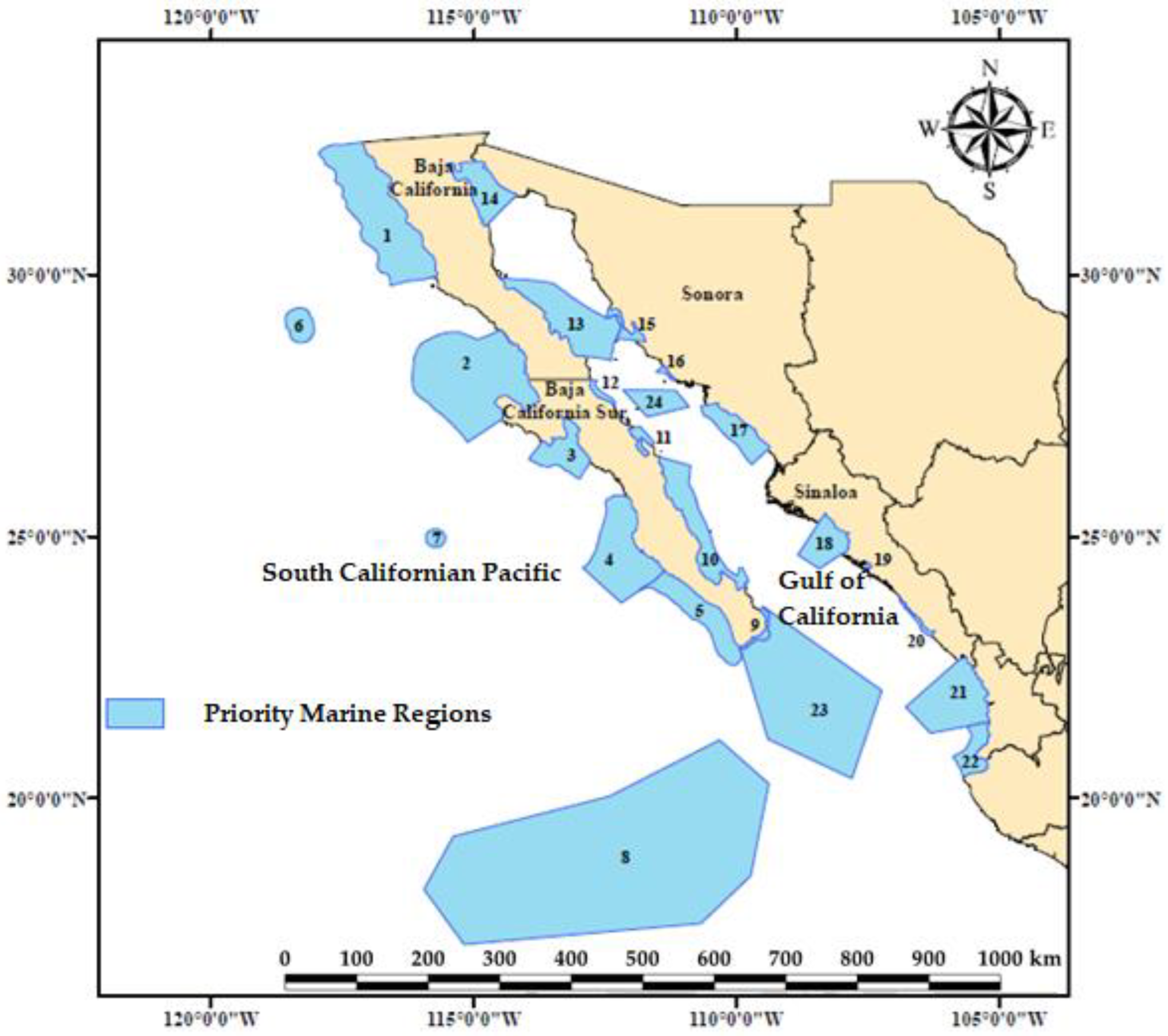
Figure 1. Map of the Priority Marine Regions (PMR) located in the Northwest of Mexico, where monthly Chlorophyll a (Chl a) data were obtained for the environmental and oceanographic analyses.
Remotesensing 14 04891 g001
Figure 2. Satellite image the Chl a monthly mean data for the 24 PMR of the Northwest of Mexico. The black boxes indicate the regions from which the chlorophyll a concentration data was obtained. The image corresponds to April 2006.
Remotesensing 14 04891 g002
Figure 3. Cluster analysis of the regions using Priority Marine Regions (PMR) of the northwest of Mexico based on monthly Chlorophyll a (Chl a) data. Linkage Distance (dotted line).
Remotesensing 14 04891 g003
Figure 4. Time series of Chlorophyll a (Chl a) concentration for the regions of the northwest of Mexico. South Californian Pacific (a); Gulf of California (b,c).
Remotesensing 14 04891 g004
Figure 5. Time series anomalies of Chlorophyll a (Chl a) for the regions of the northwest of Mexico. South Californian Pacific (a); Gulf of California (b,c).
Remotesensing 14 04891 g005
Figure 6. Variability of Chl a concentration during March and August 2011 (a,b) (La Niña), where high concentration ca be observed along the western coast of the Baja California Peninsula (South Californian Pacific) and in the Gulf of California for March, contrary to August where a clear decrease is observed. However, (c,d) corresponds to the Chl a concentration of March and August 2015 (El Niño) where a significant decrease is observed for the two months along the western coast of the Baja California Peninsula (South Californian Pacific) and in the Gulf of California in comparison with 2011. This general pattern describes the variability of Chl a concentration observed in the time series (Figure 4) and time series anomalies (Figure 5).
Remotesensing 14 04891 g006
Figure 7. Fourier analyses of Chlorophyll a (Chl a) concentration for the regions of the northwest of Mexico (Group 1, Group 2, Group 3, Group 4, San Ignacio, and Los Cabos).
Remotesensing 14 04891 g007
Figure 8. Fourier analyses of Chlorophyll a (Chl a) concentration for the regions of the Northwest of Mexico (Concepción Bay, Eastern Vizcaíno Coast, Baja California Complex Island, Upper Gulf, Infiernillo Channel and Cajón del Diablo).
Remotesensing 14 04891 g008
Figure 9. Fourier analyses of Chlorophyll a (Chl a) concentration for the regions of the northwest of Mexico (Southern Sonora Lagoon System, Santa María La Reforma Lagoons, Chiricahueto Lagoon, Piaxtla-Urías, Marismas Nacionales and Banderas Bay).
Remotesensing 14 04891 g009
Figure 10. Box-whisker plots for monthly Chlorophyll a (Chl a) concentrations in different seasons during the interannual events for Piaxtla-Urías region of the Northwest of Mexico.
Remotesensing 14 04891 g010
Table 1. List of geographic coordinates of the Priority Marine Regions (PMR) in the Northwest of Mexico. South Californian Pacific and Gulf of California.
NumberArea in Pixels (Km2)Priority Marine RegionLatitudeLongitude
147,157Ensenada32°31′48″ to 29°45′36″N117°58′12″ to 115°42′W
244,049Vizcaíno28°57′36″ to 26°47′24″N116°10′48″ to 113°43′48″W
39410San Ignacio27°18′36″ to 26°4′48″N114°1′48″ to 112°46′48″W
425,724Magdalena Bay25°47′24″ to 23°43′48″N112°55′48″ to 111°21′36″W
530,501Barra de Malva-Cabo Falso24°21′ to 22°30′36″N111°51′ to 109°54′36″W
63797Guadalupe Island29°22′12″ to 28°42′ N118°36′ to 118°2′24″W
72829Alijos Rock25°08′24″ to 24°46′12″N115°55′48″ to 115°32′24″W
8262,849Revillagigedo Islands21°05′24″ to 17°24′00″N115°57′36″ to 109°30′00″W
92171Los Cabos23°39′ to 22°49′48″N109°57′36″ to 109°21′36″W
1037,965Baja California Sur Island Complex26°31′48″ to 23°41′24″N111°28′12″ to 109°47′24″W
111780Concepción Bay27°07′12″ to 26°31′48″N112°05′24″ to 111°33′W
121751Eastern Vizcaíno Coast27°59′24″ to 27°29′24″N112°47′24″ to 112°18′36″W
1319,220Baja California Island Complex29°57′36″ to 28°31′36″N114°31′48″ to 112°12′36″W
145093Upper Gulf32°10′12″ to 30°55′48″N115°31′48″ to 114°11′24″W
151270Infiernillo Channel29°22′12″ to 28°43′48″N112°28′48″ to 111°43′48″W
16853Cajón del Diablo28°16′48″ to 27°58′48″W111°33′ to 111°09′36″W
179632Southern Sonora Lagoon System27°34’12″ to 26°21′36″N110°41′24″ to 109°21′36″W
188460Santa María La Reforma Lagoons25°26′24″ to 24°22′12″N108°51′ to 107°49′48″W
198460Chiricahueto Lagoon24°29′24″ to 24°49′48″N107°33′ to 107°25′48″W
202911Piaxtla-Urías23°48′ to 23°5′24″N106°55′48″ to 106°13′48″W
2119,424Marismas Nacionales22°41′24″ to 21°14′24″N106°47′24″ to 105°9′36″W
227219Banderas Bay21°27′36″ to 20°23′24″N105°54′ to 105°11′24″W
2375,088Entrance of the Gulf22°51′ to 20°22′48″N109°56′24″ to 107°14′24″W
246597Guaymas27°49′12″ to 27°17′24″N112°09′36″ to 110°54′36″W
Table 2. Pairwise Permutation Test for the mean monthly spring chlorophyll a (Chl a) values during El Niño and La Niña events, as well as in normal conditions, in the regions of the Northwest Pacific Ocean, Mexico. Columns sharing the same letter (for a fixed row) are not statistically different.
NumberRegionEl Niño
Event
La Niña
Event
Normal
Conditions
1Group 1 (Ensenada and Vizcaíno)2.663.793.52
2Group 2 (Baja California Sur Island Complex and Guaymas)2.983.423.50
3Group 3 (Isla Guadalupe, Alijos Rocks, Revillagigedo Islands and Gulf Entrance)0.44 (a, b)0.53 (a)0.43 (b)
4Group 4 (Magdalena Bay and Barra de Malva-Cabo Falso)3.123.963.81
5San Ignacio6.528.297.83
6Los Cabos1.552.031.60
7Concepción Bay5.166.366.27
8Eastern Vizcaíno Coast7.577.026.84
9Baja California Island Complex9.778.577.90
10Upper Gulf9.998.868.50
11Infiernillo Channel15.9417.1017.68
12Cajón del Diablo6.699.1310.26
13Southern Sonora Lagoon System4.987.098.75
14Santa María La Reforma Lagoons6.049.0410.76
15Chiricahueto Lagoon15.6220.3921.31
16Piaxtla-Urías4.009.508.80
17Marismas Nacionales2.307.423.41
18Banderas Bay5.2116.207.26
Table 3. Pairwise Permutation Test for the mean monthly summer chlorophyll a (Chl a) values during El Niño and La Niña events, as well as in normal conditions, in the regions of the Northwest Pacific Ocean, Mexico. Columns sharing the same letter (for a fixed row) are not statistically different.
NumberRegionEl Niño
Event
La Niña
Event
Normal
Conditions
1Group 1 (Ensenada and Vizcaíno)2.382.342.39
2Group 2 (Baja California Sur Island Complex and Guaymas)1.411.711.52
3Group 3 (Isla Guadalupe, Alijos Rocks, Revillagigedo Islands and Gulf Entrance)0.420.400.39
4Group 4 (Magdalena Bay and Barra de Malva-Cabo Falso)3.293.753.87
5San Ignacio9.258.859.24
6Los Cabos1.701.881.96
7Concepción Bay2.303.112.56
8Eastern Vizcaíno Coast3.563.543.78
9Baja California Island Complex3.444.393.85
10Upper Gulf6.987.546.68
11Infiernillo Channel8.1110.7010.37
12Cajón del Diablo1.132.401.81
13Southern Sonora Lagoon System1.872.882.33
14Santa María La Reforma Lagoons2.874.043.24
15Chiricahueto Lagoon10.7312.4611.65
16Piaxtla-Urías2.11 (a, b)3.52 (a)2 (b)
17Marismas Nacionales2.54 (a, b)3.40 (a)1.83 (b)
18Banderas Bay2.86 (a)3.49 (a)1.84 (b)
Table 4. Pairwise Permutation Test for the mean monthly autumn chlorophyll a (Chl a) values during El Niño and La Niña events, as well as in normal conditions, in the regions of the Northwest Pacific Ocean, Mexico. Columns sharing the same letter (for a fixed row) are not statistically different.
NumberRegionEl Niño
Event
La Niña
Event
Normal Conditions
1Group 1 (Ensenada and Vizcaíno)1.271.521.23
2Group 2 (Baja California Sur Island Complex and Guaymas)1.72 (a, b)1.93 (a)1.47 (b)
3Group 3 (Isla Guadalupe, Alijos Rocks, Revillagigedo Islands and Gulf Entrance)0.440.390.36
4Group 4 (Magdalena Bay and Barra de Malva-Cabo Falso)0.811.120.95
5San Ignacio1.772.321.98
6Los Cabos0.590.800.71
7Concepción Bay3.314.564.45
8Eastern Vizcaíno Coast5.655.865.58
9Baja California Island Complex4.554.664.32
10Upper Gulf7.608.447.10
11Infiernillo Channel12.3313.0413.42
12Cajón del Diablo4.764.744.37
13Southern Sonora Lagoon System3.29 (a)4.60 (b)3.51 (a)
14Santa María La Reforma Lagoons3.82 (a)5.54 (b)4.48 (a, b)
15Chiricahueto Lagoon17.5920.0718.00
16Piaxtla-Urías3.18 (a)4.91 (b)3.54 (a, b)
17Marismas Nacionales2.443.842.65
18Banderas Bay1.835.352.99
Table 5. Pairwise Permutation Test for the mean monthly winter chlorophyll a (Chl a) values during El Niño and La Niña events, as well as in normal conditions, in the regions of the Northwest Pacific Ocean, Mexico. Columns sharing the same letter (for a fixed row) are not statistically different.
NumberRegionEl Niño
Event
La Niña
Event
Normal Conditions
1Group 1 (Ensenada and Vizcaíno)1.34 (a)2.10 (b)1.54 (a, b)
2Group 2 (Baja California Sur Island Complex and Guaymas)3.163.543.27
3Group 3 (Isla Guadalupe, Alijos Rocks, Revillagigedo Islands and Gulf Entrance)0.50 (a, b)0.65 (a)0.47 (b)
4Group 4 (Magdalena Bay and Barra de Malva-Cabo Falso)1.03 (a)1.67 (b)1.30 (a, b)
5San Ignacio1.87 (a)2.93 (b)2 (a)
6Los Cabos1.592.641.87
7Concepción Bay6.117.748.07
8Eastern Vizcaíno Coast3.964.765.44
9Baja California Island Complex4.035.155.18
10Upper Gulf6.958.408.01
11Infiernillo Channel12.9415.8317.45
12Cajón del Diablo5.936.557.41
13Southern Sonora Lagoon System6.117.307.00
14Santa María La Reforma Lagoons6.308.568.23
15Chiricahueto Lagoon15.2218.4319.87
16Piaxtla-Urías5.22 (a)10.59 (b)6.31 (a)
17Marismas Nacionales2.30 (a)5.22 (b)2.78 (a)
18Banderas Bay3.07 (a)7.98 (b)4.36 (a)
Publisher’s Note: MDPI stays neutral with regard to jurisdictional claims in published maps and institutional affiliations.

