Estimation of Swell Height Using Spaceborne GNSS-R Data from Eight CYGNSS Satellites

Abstract

Global Navigation Satellite System (GNSS)-Reflectometry (GNSS-R) technology has opened a new window for ocean remote sensing because of its unique advantages, including short revisit period, low observation cost, and high spatial-temporal resolution. In this article, we investigated the potential of estimating swell height from delay-Doppler maps (DDMs) data generated by spaceborne GNSS-R. Three observables extracted from the DDM are introduced for swell height estimation, including delay-Doppler map average (DDMA), the leading edge slope (LES) of the integrated delay waveform (IDW), and trailing edge slope (TES) of the IDW. We propose one modeling scheme for each observable. To improve the swell height estimation performance of a single observable-based method, we present a data fusion approach based on particle swarm optimization (PSO). Furthermore, a simulated annealing aided PSO (SA-PSO) algorithm is proposed to handle the problem of local optimal solution for the PSO algorithm. Extensive testing has been performed and the results show that the swell height estimated by the proposed methods is highly consistent with reference data, i.e., the ERA5 swell height. The correlation coefficient (CC) is 0.86 and the root mean square error (RMSE) is 0.56 m. Particularly, the SA-PSO method achieved the best performance, with RMSE, CC, and mean absolute percentage error (MAPE) being 0.39 m, 0.92, and 18.98%, respectively. Compared with the DDMA, LES, TES, and PSO methods, the RMSE of the SA-PSO method is improved by 23.53%, 26.42%, 30.36%, and 7.14%, respectively.

1. Introduction

Swell height information is of much concern in the design of coastal structures and ocean platforms, navigation safety, and offshore engineering [1]. The traditional method for swell height in situ measurement is to place buoys on the sea surface to collect the surrounding information, which has the advantages of being fixed, long-term, and timely. However, it has limited coverage, involves high cost, and is easily affected by environmental factors. A second way to obtain swell height is using a satellite altimeter. This technique has been widely investigated in previous studies [2,3,4], and it can provide swell height data at global coverage and climate scales; however, the spatial resolution of the existing satellite altimeter is limited. Synthetic aperture radar (SAR) altimetry data have become a new source for swell monitoring [5,6], as well as for swell heigh measurement [7,8,9]. However, this kind of observation is sparse in both time and space. Numerical models compensate for these limitations eventually at the expense of additional errors imparted by inaccurate physical processes, such as dissipation [10], and by forcing uncertainties.

High-frequency radar (HFR) offers another way to monitor ocean swell [11,12,13,14]. These HFRs are land-based ground-wave radars. They collect ocean surface information continuously in near-real time over a large area (~100 km) and with high spatial (~1 km) and temporal (~1 h) resolutions. Swell height measurement by HFR technique was investigated in recent years [15,16]. Since the wind wave and swell patterns can be presented on X-band radar images, X-band radar is also an effective tool for obtaining swell height information [17,18]. However, wind waves and swell cannot be imaged well by X-band radar under nononshore wind conditions [19]. Additionally, unlike HFR and satellite measurements, which can monitor up to several hundred square kilometers or even almost global areas, the effective measuring area for ocean swell by the X-band radar is limited to dozens of square kilometers [20].

In recent years, with the launch of many satellites, GNSS technology has developed rapidly. GNSS satellites can provide all-weather, all-day, uninterrupted L-band microwave signal sources, which can offer navigation, positioning, and accurate timing information to users on the earth. As a new remote sensing technology, Global Navigation Satellite System-Reflectometry (GNSS-R) has been intensively investigated in marine remote sensing in recent years because of its unique advantages of short revisit period, low observation cost, and high spatial-temporal resolution, for example, sea surface wind speed retrieval [21,22], sea surface height retrieval [23], sea ice detection [24], tsunami detection [25], and rainfall detection and intensity retrieval [26,27,28,29]. In the past eight years, several GNSS-R mission satellites have been launched, such as the TechDemosat-1 (TDS-1) satellite [30] from the United Kingdom, Cyclone GNSS (CYGNSS) satellites [31] from the United States and BuFeng-1 A/B satellites [32] from China, ESA’s FSSCat satellites (³Cat-5/A and ³Cat-5/B satellites) [33] and the FY-3E satellite of the China Meteorological Administration [34]. Accordingly, spaceborne GNSS-R data have also been used for significant wave height (SWH) (Hs) retrieval, although only a few results are reported [35,36,37,38,39,40]. Unfortunately, there is no research on estimating swell height by using spaceborne GNSS-R data.

This paper aims to study the potential of GNSS-R in swell height estimation by using the observables obtained from the GNSS-R delay-Doppler map (DDM). The main contributions in this article are summarized as follows:

(1)

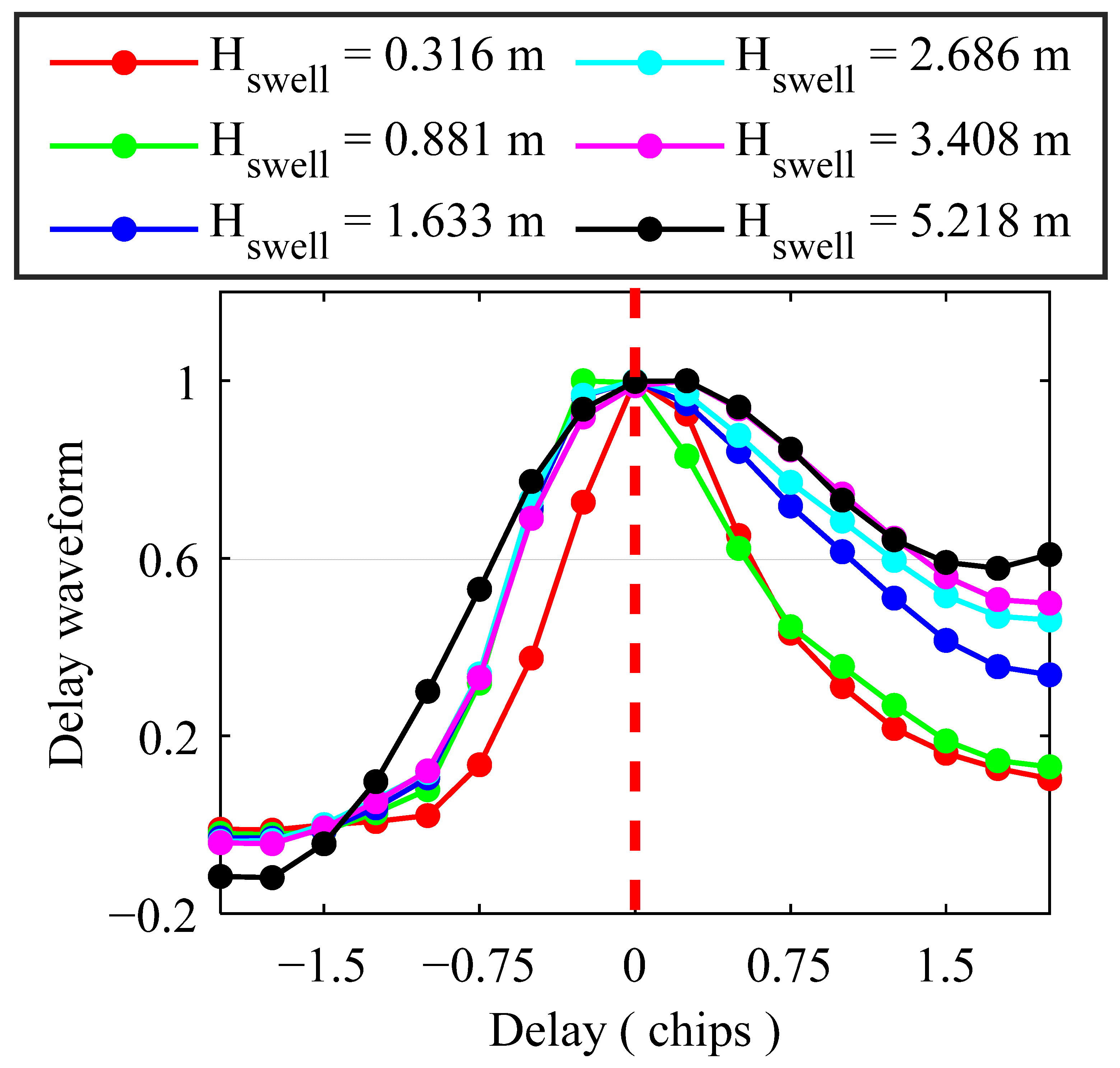
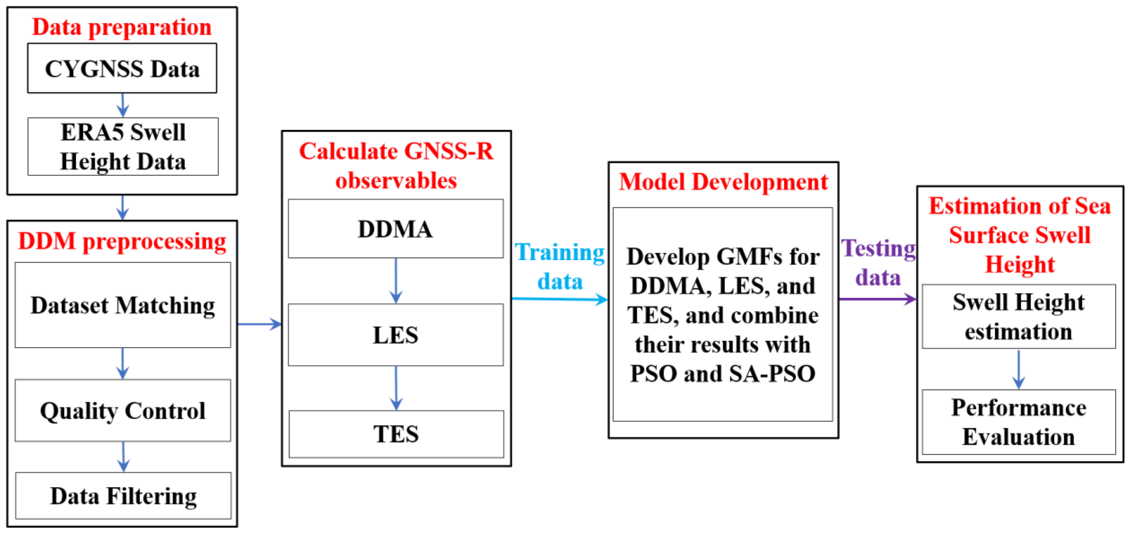
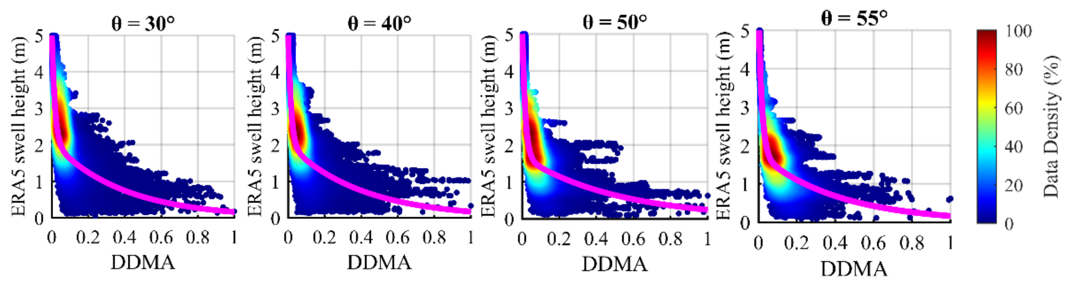
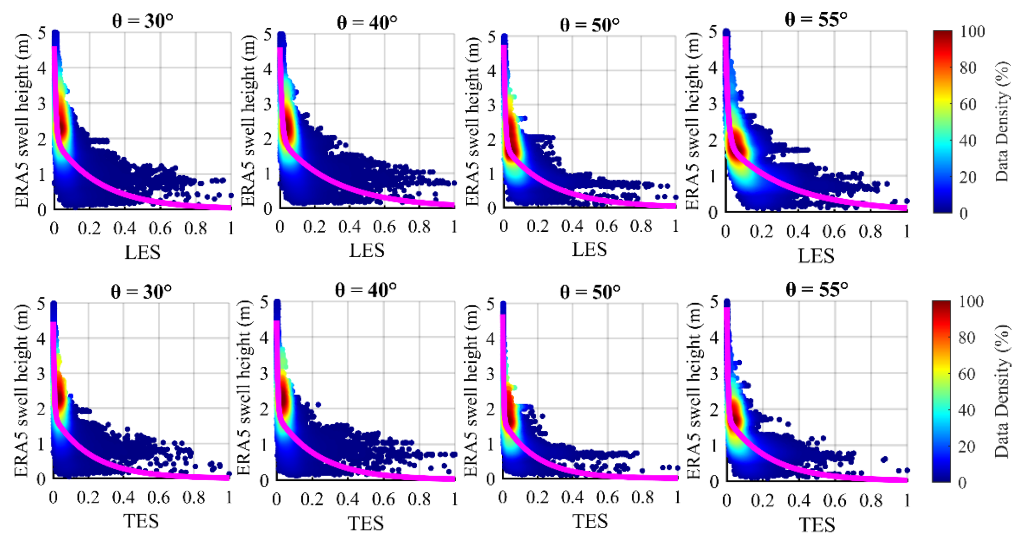
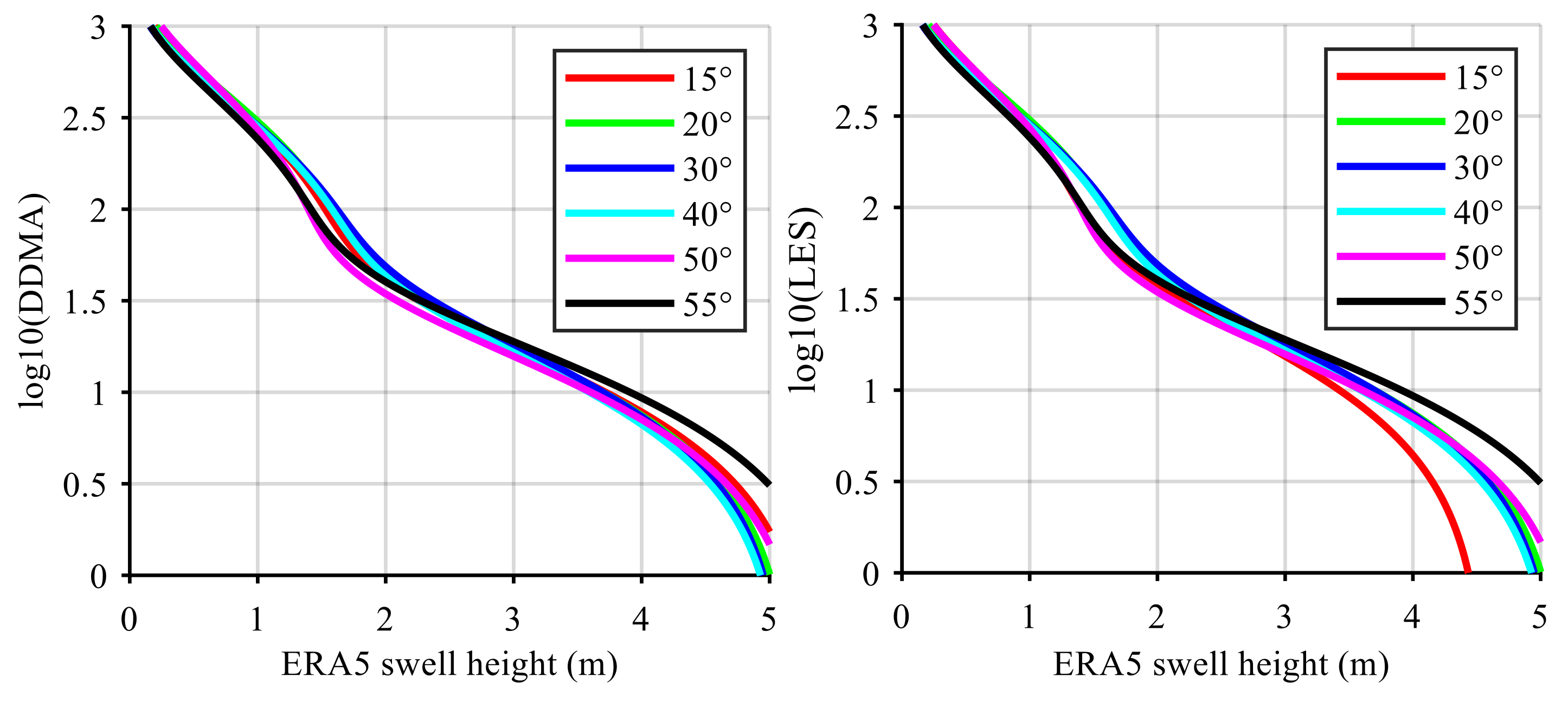
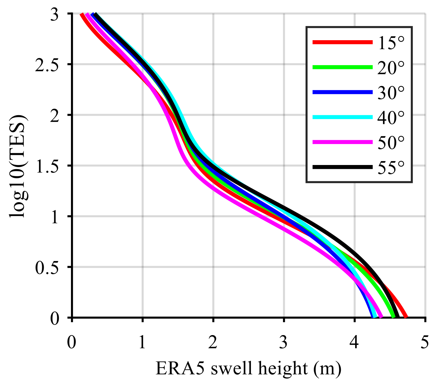
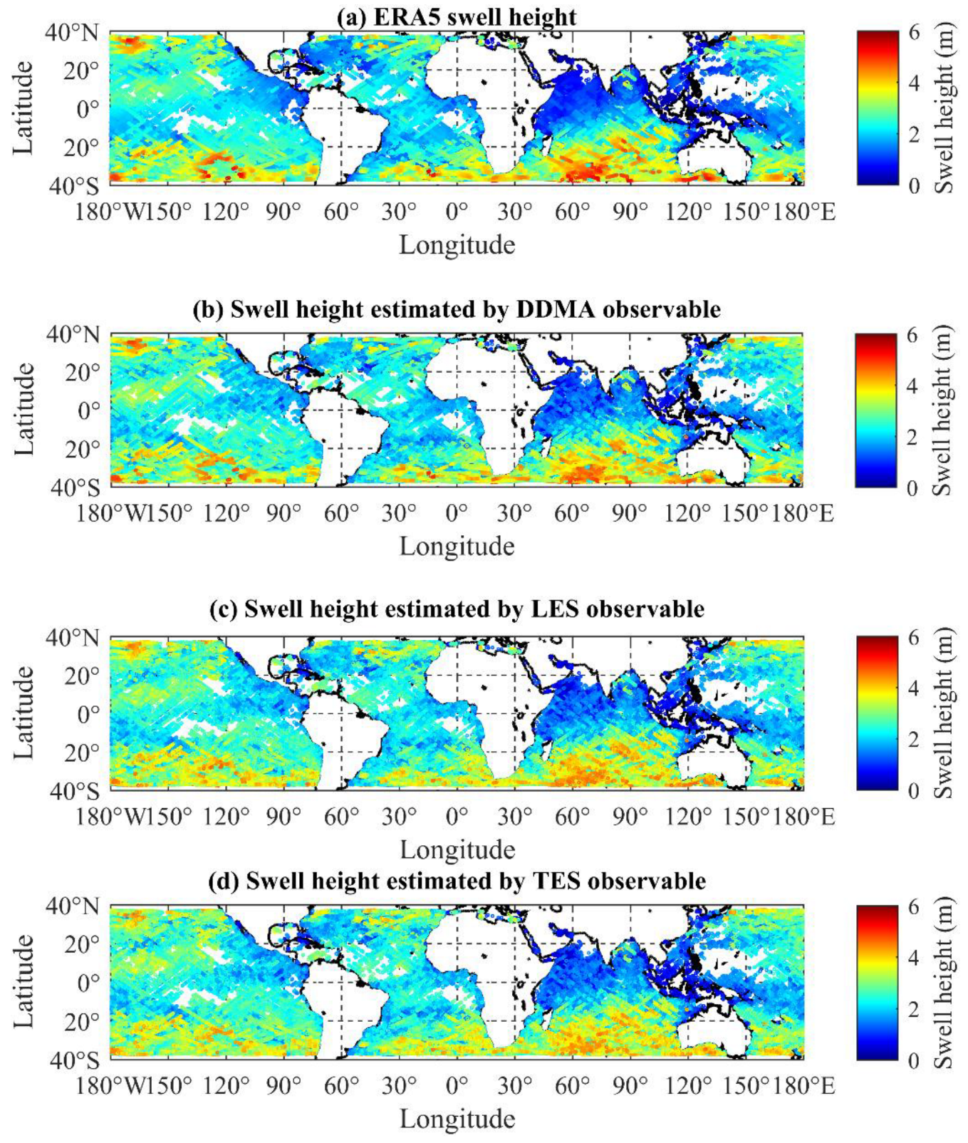
Three GNSS-R observables extracted from DDM were introduced and used for swell height estimation, i.e., delay-Doppler map average (DDMA), the leading edge slope (LES) of the integrated delay waveform (IDW), and the trailing edge slope (TES) of the IDW.

(2)

Based on these three GNSS-R observables, empirical models were developed for retrieving swell height.

(3)

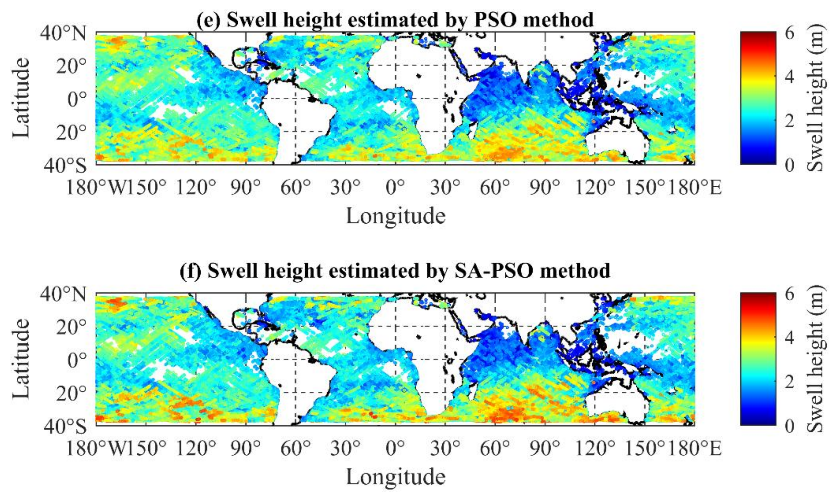
Particle swarm optimization (PSO) was exploited to establish a combined model to enhance the swell height estimation performance.

(4)

The problem of local optimal solutions often occurs in the PSO algorithm. To overcome the problem and further increase the measurement accuracy, we proposed a SA-PSO algorithm that combines simulated annealing and PSO.

The structure of this paper is described as follows: Section 2 describes the data sets and data processing strategy. Section 3 introduces the swell height estimation model in detail, and Section 4 shows the evaluation results with the ERA5 swell height product as a reference and gives the discussions. Finally, Section 5 draws the conclusion in this paper.

2. Dataset Description and Data Processing

2.1. Data

To develop the swell height retrieval model and test the performance of the model, two data sets were used, which are GNSS-R data from CYGNSS L1 V3.0 product and reanalysis swell height datasets from the ECMWF (European Center for Medium-Range Weather Forecasts).

(1) CYGNSS GNSS-R data

CYGNSS consists of eight micro-satellites, each with four delay-Doppler mapping instruments (DDMI) that generate DDM data. The original DDM size (i.e., number of pixels) of CYGNSS is 20 × 128 (20 Doppler shifts and 128 time delays). To facilitate data transmission, the size of DDM is compressed to 11 × 17. At the moment, NASA’s PODAAC (Physical Oceanography Distributed Active Archive Center) mainly open three levels (i.e., level 1, level 2, and level 3) of CYGNSS GNSS-R data to users for free. In this article, we use L1 V3.0 data product downloaded from the website https://podaac-tools.jpl.nasa.gov/drive/files/allData/cygnss/L3/v3.0 (accessed on 1 January 2022), which includes DDM, specular reflection point positions, and transmitter positions of eight CYGNSS satellites. The current version mainly contains GNSS-R data for the period from 1 August 2018 (day of year (DOY) is 213) to 2021. Considering the large amount of data, we only downloaded the CYGNSS data from 1 April 2019 to 31 July 2019 for our study, corresponding to DOY of 091~212.

(2) ECMWF reanalysis swell height datasets

The Copernicus Climate Change Service (C3S) Climate Database provides users with free access to the ECMWF reanalysis data product (https://www.ecmwf.int/en/forecasts/datasets/browse-reanalysis-datasets (accessed on 1 January 2022)). The ECMWF ERA5 data are the latest product, which provide waves height data with a spatial resolution of 0.5° × 0.5° and a time resolution of 1 h. The ERA5 reanalysis product provides three types of waves height data, i.e., wind waves height, swell height, and height of combined wind waves and swell. The wind wave and swell components are separated by means of spectral analysis [41]. In this study, the swell height data was chosen for model design and validation. Considering the spatial–temporal resolution difference between the CYGNSS GNSS-R data and the ERA5 swell height data, the ERA5 swell height data had to be collocated with the CYGNSS data. A linear interpolation in time and a bilinear interpolation in space were used to obtain the co-located swell height.

2.2. Data Quality Control

The CYGNSS L1 version 3.0 measurements are quality controlled before model construction and verification based on the following criteria [42,43,44]:

(a)

The observables must be positive, while the Nan values need to be discarded.

(b)

When the star tracker is unable to track due to solar contamination, the measurements taken are discarded.

(c)

The uncertainty of the bistatic radar cross section (BRCS) is below 1.

(d)

The nano star tracker attitude status is set to 0; it shows that the nano star tracker attitude status is “OK”.

(e)

When the absolute value of spacecraft roll is greater than 30 degrees, the yaw is greater than 5 degrees, and the pitch is greater than 10 degrees, the measurement values are discarded.

(f)

The observables from GPS IIF satellites are removed, because accurate information on the transmitter antenna gain pattern of GPS satellites was not available.

(g)

The DDM data with the range corrected gain (RCG) figure of merit (FOM) for the DDM (prn_fig_of_merit) less than 0 are discarded.

(h)

The observation data with the receive antenna gain (sp_rx_gain) in the direction of the specular reflection point less than 0 dBi are discarded.

(i)

In order to reduce land effects and modeling error, observations with specular reflection points greater than 25 km from land were selected.

(j)

Observable data range is defined as 38°N–38°S in the latitude.

(k)

For more descriptions, see the CYGNSS L1 V3.0 users’ guide and data dictionary, which can be found on the Web site (https://podaac-tools.jpl.nasa.gov/drive/files/allData/cygnss/L1/docs/148-0346-8_L1_v3.0_netCDF_Data_Dictionary.xlsx (accessed on 1 January 2022)).

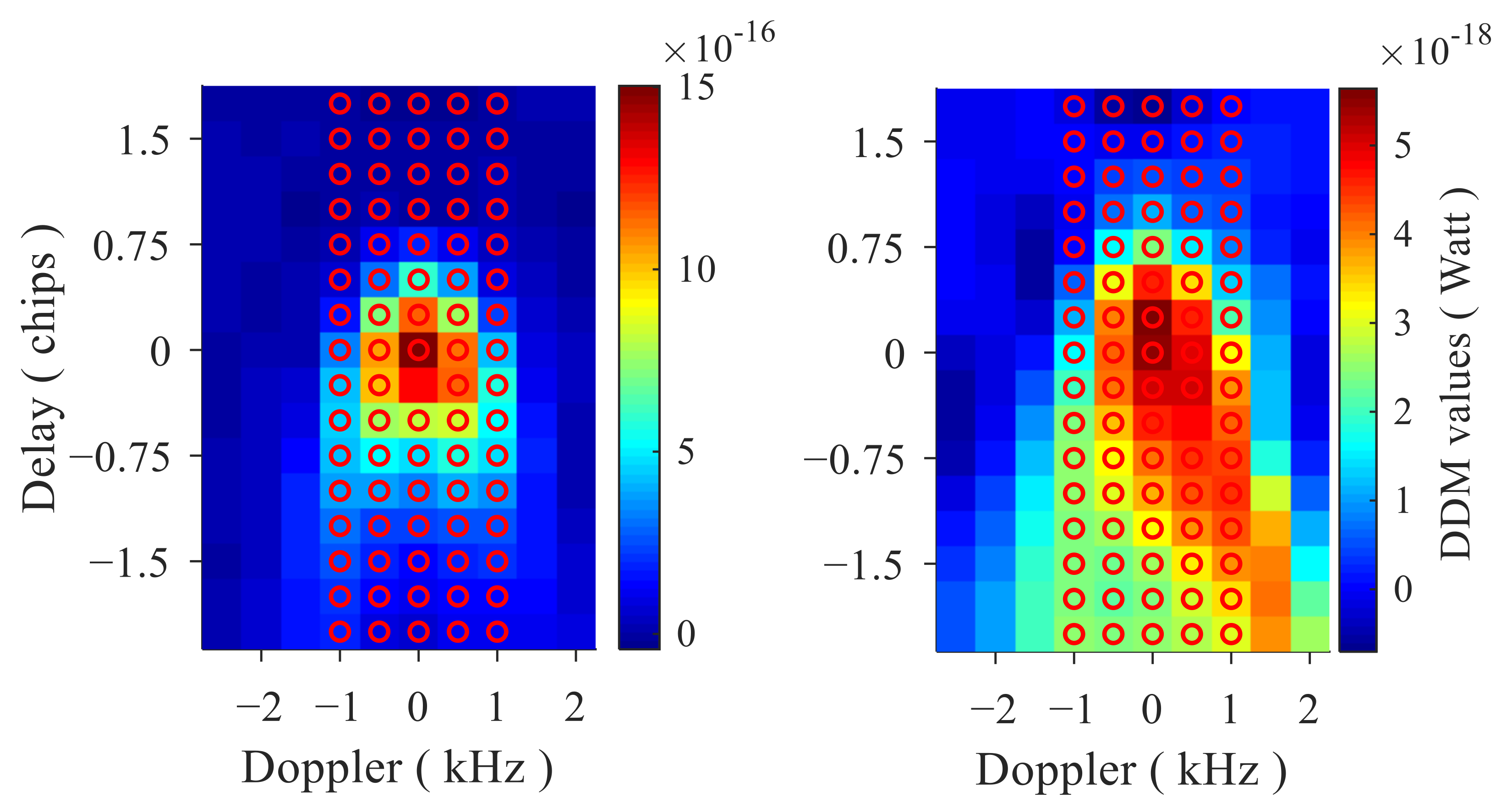
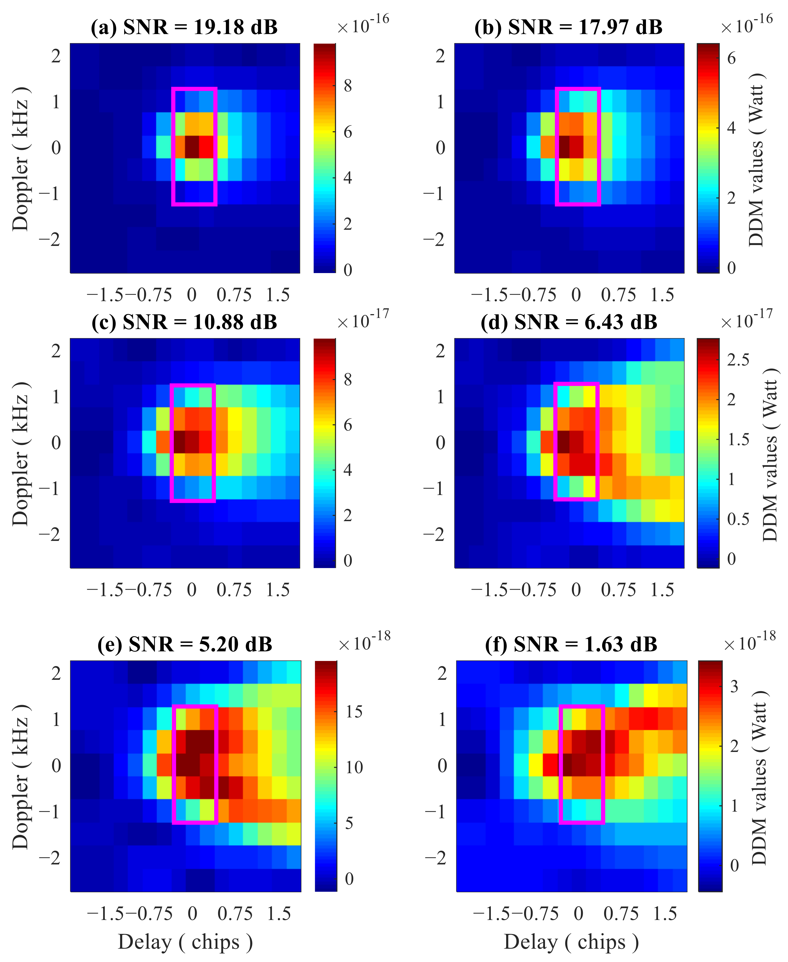
2.3. Spaceborne GNSS-R DDM and Integral Delay Waveforms

The power model of the GNSS scattered signal is proposed by Zavorotny and Voronovich based on the KA-GO (Kirchhoff approximation to geometric optics) [45]; it describes scattered GNSS signal power as a function of geometrical, environmental, and system parameters. The model can be used to generate the DDM, which has since been widely studied. In this study, DDMs were also used for swell height retrieval.

When the time-delay waveforms corresponding to Doppler frequency within a certain range are accumulated and averaged, the integral delay waveform (IDW) is generated as [46]:

$${\omega }_{IDW}(\tau )=\frac{1}{N}{\displaystyle \sum _{l=1}^N〈{\left|Y^{\prime }(\tau ,f_l)\right|}^2〉}$$

(1)

where ${\omega }_{IDW}(\tau )$ is the IDW; $N$ is the number of Doppler frequency shifts, and it is set to 5; $〈{\left|Y^{\prime }(\tau ,f_l)\right|}^2〉$ is the power of the reflected signal after removing the average noise level when the time delay and Doppler shift are $\tau$ and $f_l$, respectively.

To clearly explain the calculation method of the IDW, Figure 1 shows two examples of DDM pixels from selected Doppler shifts and time delays used to calculate IDW. The IDW is generated by summing the five-pixel values of five different Doppler shifts (i.e., [−1000 1000] Hz) for each time delay.

2.4. Definition of GNSS-R Observables

In previous studies, several DDM-related observables such as SNR, delay-Doppler map average (DDMA), Woodward ambiguity function (WAF) matched filter (MF), trailing edge slope (TES), and normalized bistatic radar scattering cross section (NBRCS) have been proposed for different GNSS-R applications, e.g., sea surface wind speed retrieval [31], sea ice monitoring [47], and soil moisture retrieval [48]. In this study, the DDMA and two observables (leading edge slope (LES) and TES) derived from the integral delay waveforms are used for swell height estimation. These three observables are defined as follows:

(1) DDMA: DDMA is the average scattering power of a specific time-delay Doppler window of DDM near the specular reflection point, expressed as:

$$DDMA=\frac{1}{k\times j}{\displaystyle \sum _{p=8}^{10}{\displaystyle \sum _{q=4}^{8}DDM({\tau }_p,f_q)}}$$

(2)

where $DDM({\tau }_p,f_q)$ is the power (pixel value or DDM value) after denoising when time delay and Doppler shift are ${\tau }_p$ and $f_q$, respectively. Pixel values of $k$ time delays and $j$ Doppler shifts centered at the peak DDM are used to determine the DDMA. In this work, $k$ = 3 and $j$ = 5.

(2) Leading Edge Slope (LES) of Integrated Delay Waveforms (LES-IDW): Taking the time delay as the 0 chips dividing point, we selected a certain number of integral delay waveform values in the time delay window of the leading edge part and calculated the leading edge slope of IDW by least square fitting, expressed as follows:

$$LES=\frac{n{\displaystyle \sum _{i=1}^n{\tau }_i^L{\omega }_{IDW,i}^L}-{\displaystyle \sum _{i=1}^n{\tau }_i^L{\displaystyle \sum _{i=1}^n{\omega }_{IDW,i}^L}}}{n{\displaystyle \sum _{i=1}^n{({\tau }_i^L)}^2-{({\displaystyle \sum _{i=1}^n{\tau }_i^L})}^2}}$$

(3)

where $IDW$ represents the integrated delay waveform, ${\omega }_{IDW,i}^L$ is the leading waveform value of IDW, ${\tau }_i^L$ is the time delay value of the leading edge, $n$ is the number of delay bins for curve fitting, IDW is calculated as described in Section 2.3.

(3) Trailing Edge Slope (TES) of Integrated Delay Waveforms (TES-IDW): Taking the time delay as the 0 chips dividing point, we selected a certain number of integral delay waveform values in the time delay window of the trailing edge part and calculated the trailing edge slope of IDW by least square fitting, that is:

$$TES=\frac{n{\displaystyle \sum _{i=1}^n{\tau }_i^T{\omega }_{IDW,i}^T}-{\displaystyle \sum _{i=1}^n{\tau }_i^T{\displaystyle \sum _{i=1}^n{\omega }_{IDW,i}^T}}}{n{\displaystyle \sum _{i=1}^n{({\tau }_i^T)}^2-{({\displaystyle \sum _{i=1}^n{\tau }_i^T})}^2}}$$

(4)

where ${\omega }_{IDW,i}^T$ is the trailing edge value of IDW, ${\tau }_i^T$ is the time delay of the trailing edge. The definitions of other symbols are the same as (3).

Note that an important aspect of calculating DDMA, TES, and LES observables from DDMs is to calculate the delay and Doppler range of the observables. DDMA, LES, and TES observables were calculated using the same Doppler and delay window, and the Doppler and delay ranges were determined to be [−1000 1000] Hz and [−0.25 0.25] chips, respectively, corresponding to a 5 × 3 window around the specular point in DDM (as shown in the magenta box in Figure 2). This choice is based on the consideration that averaging more diffuse scattering signals will improve SNR without reducing the spatial resolution incurred using a larger integration region [31].

For the convenience of illustration and calculation, the zero time-delay point is used as the demarcation point of the leading edge (LE) part and trailing edge (TE) part. Figure 2 and Figure 3, respectively, show the DDM and NIDW of different swell heights with different SNR values. The CYGNSS DDM data used were collected on the ocean on 30 April 2019. As shown in the figure, the integrated delay waveforms of the reflected signals have different characteristics under different swell heights, which provides a new opportunity for remote sensing technology to retrieve swell height.

3. Model Construction

3.1. Basic Description

First, the CYGNSS data are preprocessed and selected as mentioned previously. Then, the three DDM-based observables are calculated, and a linear interpolation in time and a bilinear interpolation in space are applied to the ERA5 swell height products to match the DDM data acquisition time and the positions of specular points. The data are further randomly divided into two parts of equal size, one for the training data set and the other for the test data set. One of the three observables and swell height are treated as input and output variables, respectively, of one individual model established by least-squares fitting. To enhance the swell height retrieval performance, two different data fusion schemes are proposed to combine the estimates based on the three individual observables. The two fusion schemes are particle swarm optimization (PSO) and simulated annealing aided PSO (SA-PSO). The swell height retrieval results based on the five schemes (i.e., DDMA method, LES method, TES method, PSO method, and SA-PSO method) are compared with the ERA5 swell height product data for performance evaluation. Figure 4 depicts the algorithm of the model development and testing process.

3.2. Modeling Based on Individual Observables

In this section, we used the DDMA, LES, and TES observables to develop the swell height estimation models. To deal with the effect of incident angle, the training data are divided into groups, each of which corresponds to a bin of incident angles with a bin width of 5 degrees. Accordingly, each group of data generates a swell height estimation model for each scheme. After processing extensive experimental data and studying the relationship between the three observables and swell height, we proposed the following model:

$$H_{swell}{}_{,ob}=a_1\exp (b_1{x}_{ob,i})+a_2\exp (b_2{x}_{ob,i})$$

(5)

where $H_{swell}{}_{,ob}$ is the swell height estimated by the model, $x_{ob,i}$ denotes any of the three observables, the other symbols are the fitting parameters of the retrieval model to be determined by the nonlinear least-squares fitting method.

To consider the dependence of the swell height retrieval on incident angle, it is very important to study the swell height modeling under different incident angles. Figure 5 shows some examples of the training dataset for the DDMA, LES, and TES observables at four different incidence angles (θ). In the figure, the scattering density points represent the corresponding relationship between GNSS-R observations and ERA5 swell height values, and the magenta solid line is the swell height retrieval empirical model fitted by the training data. The general trend is that the swell height decreases as the observable increases.

DDMA, LES, and TES observables were used to develop GMFs. Figure 6 shows the GMFs of DDMA, LES, and TES for some incidence angle bins. It can be seen that the three observables decreased rapidly with the increase in swell height. This is because with the increase in swell height, the sea surface becomes rougher, resulting in the reduction in the power of GNSS-reflected signal flatter trailing and leading edges. If the training sample is small or the DDM noise is large, the modeling error can be easily transferred to the GMF, which will inevitably amplify the observation error of the final swell height retrieval. However, in the low swell height range, the incident angle has little effect on the retrieval model, but this effect becomes significant when swell height is higher than a certain value around 4 m.

3.3. Modeling Based on PSO Method

Inspired by the wind retrievals method incorporating PSO presented in [42], a new method that combines swell height retrievals from GNSS-R observables and PSO was first introduced. The single feature value retrieval results $\widehat{w}={(w_{DDMA},w_{LES},w_{LES})}^T$ are linearly combined, where $w_{DDMA}$, $w_{LES}$, and $w_{TES}$ are the swell height estimations based on DDMA, LES, and TES, respectively; and the combination coefficient vector to be optimized is $\overrightarrow{k}=(k_{DDMA},k_{LES},k_{TES})$, where $k_{DDMA}$, $k_{LES}$, and $k_{TES}$ are the combination coefficients of DDMA, LES and TES, respectively.

The objective function of the combined swell height estimation is set as the mean square error between the combined estimation result and the reference true value $w_{True}$. The optimization objective of the particle swarm is to find a set of combined coefficients that make the objective function take a very small value in the search space, and its specific form is as follows:

$$F(\overrightarrow{k})=〈{\left(\overrightarrow{k}\cdot \widehat{w}-w_{\mathrm{True} }\right)}^2〉$$

(6)

The specific implementation steps of the PSO algorithm are as follows:

(a) In the given parameter search space, a set of particles is produced randomly according to Equation (6); the individual and global optimal points are obtained.

(b) Update the combination coefficient and the combination coefficient correction value; the specific functional form of the combination coefficient correction value is as follows;

$${\overrightarrow{\Delta k}}_{i+1}=\kappa \ast {\overrightarrow{\Delta k}}_i+c_1\ast {\mathrm{rand} }_i^1\left(pbes{t}_i-{\overrightarrow{k}}_i\right)+c_2\ast {\mathrm{rand} }_i^2\left(gbes{t}_i-{\overrightarrow{k}}_i\right)$$

(7)

where $\overrightarrow{k_i}$ is the current particle combination coefficient, $\overrightarrow{\Delta k_i}$ and $\overrightarrow{\Delta k_{i+1}}$ are the current combination coefficient correction value and the updated combination coefficient correction value, respectively. $\kappa$ is the inertia factors, $c_1$ and $c_2$ are the learning factors, $ran{d}_i^1$ and $ran{d}_i^2$ are the generated random numbers.

(c) The current particle combination coefficients $\overrightarrow{k_i}$ are corrected according to the updated combination coefficient correction value as:

$${\overrightarrow{k}}_{i+1}={\overrightarrow{k}}_i+\overrightarrow{\Delta k_{i+1}}$$

(8)

(d) The individual and global optima are updated.

(e) Determine whether the termination condition of particle swarm optimization is satisfied, and if not, repeat steps (b) and (c) until the termination condition is satisfied.

(f) The optimal combination coefficient $\overrightarrow{k}$ is taken as the one that minimizes $F(\overrightarrow{k})$ in Equation (6) and it is used for swell height estimation via:

$${\widehat{W}}_{PSO}=\overrightarrow{k}\cdot \widehat{w}$$

(9)

The advantage of the PSO algorithm is that it can use a large number of particles in a certain search space to quickly and accurately find the best set of combination coefficients that satisfy the final conditions, thus, minimizing the objective function (i.e., MSE) of the combination result relative to the true value of the swell height.

3.4. Modeling Based on Combination of Simulated Annealing and Particle Swarm Optimization (SA-PSO) Algorithm

To overcome the problem of local optimal solution of the PSO algorithm, a simulated-annealing (SA)-based particle swarm optimization (PSO) algorithm (SA-PSO) is proposed. This algorithm makes the flight of particles memoryless and enhances the global search capability by using the simulated annealing algorithm to regenerate the positions of the stopped evolving particles. At the same time, a double population search mechanism is adopted. That is, one population keeps particles with feasible solutions, and the particles are searched for the optimal feasible solution step by step by the SA-PSO algorithm; the other population keeps particles with infeasible solutions, and the feasible solution population accepts particles with infeasible solutions with a certain probability, which not only improves the search capability and search efficiency of the algorithm, but also effectively keeps the population diversity and improves the local search ability of the PSO algorithm.

The specific implementation steps of the SA-PSO algorithm are as follows:

(a) Each particle in the population is given a random starting position and velocity.

(b) The fitness of each particle is calculated. The current position and fitness value of each particle are stored in the corresponding $p_i$, and the position and fitness value of the individual with the best fitness value in all pbest are stored in $p_g$.

(c) The initial temperature is determined according to the following equation:

$$t_0=f\left(p_g\right)/\ln 5$$

(10)

(d) At current temperature, the fitness value of each $p_i$ is calculated using the following equation:

$$TF\left(p_i\right)=\frac{e^{-\left[f\left(p_i\right)-f\left(p_g\right)\right]/t}}{{\displaystyle \sum _{i=1}^N{e}^{-\left[f\left(p_i\right)-f\left(p_g\right)\right]/t}}}$$

(11)

(e) A roulette strategy is used to determine the global optimum of some alternative from all, and then the velocity and position of each particle are updated according to the following formula:

$$\left\{\begin{array}{l}{v}_{i,j}(t+1)=\phi \left\{v_{i,j}(t)+c_1{r}_1\left[p_{i,j}-x_{i,j}(t)\right]+c_2{r}_2\left[p_{g,j}^{\prime }-x_{i,j}(t)\right]\right\}\\ x_{i,j}(t+1)=x_{i,j}(t)+v_{i,j}(t+1)\end{array}\right.$$

(12)

where $\phi =2/\left|2-C-\sqrt{C^2-4C}\right|$, $C=c_1+c_2$.

(f) Calculate the new target value for each particle and update the value $p_i$ for each particle and the value for the population $p_g$.

(g) Perform the annealing operation according to the following equation:

$$t_{k+1}=\lambda t_k$$

(13)

where $\lambda$ is the annealing constant.

(h) If the stop condition is satisfied, the search stops, and the results are output; otherwise, turn to step (d).

4. Model Performance Evaluation

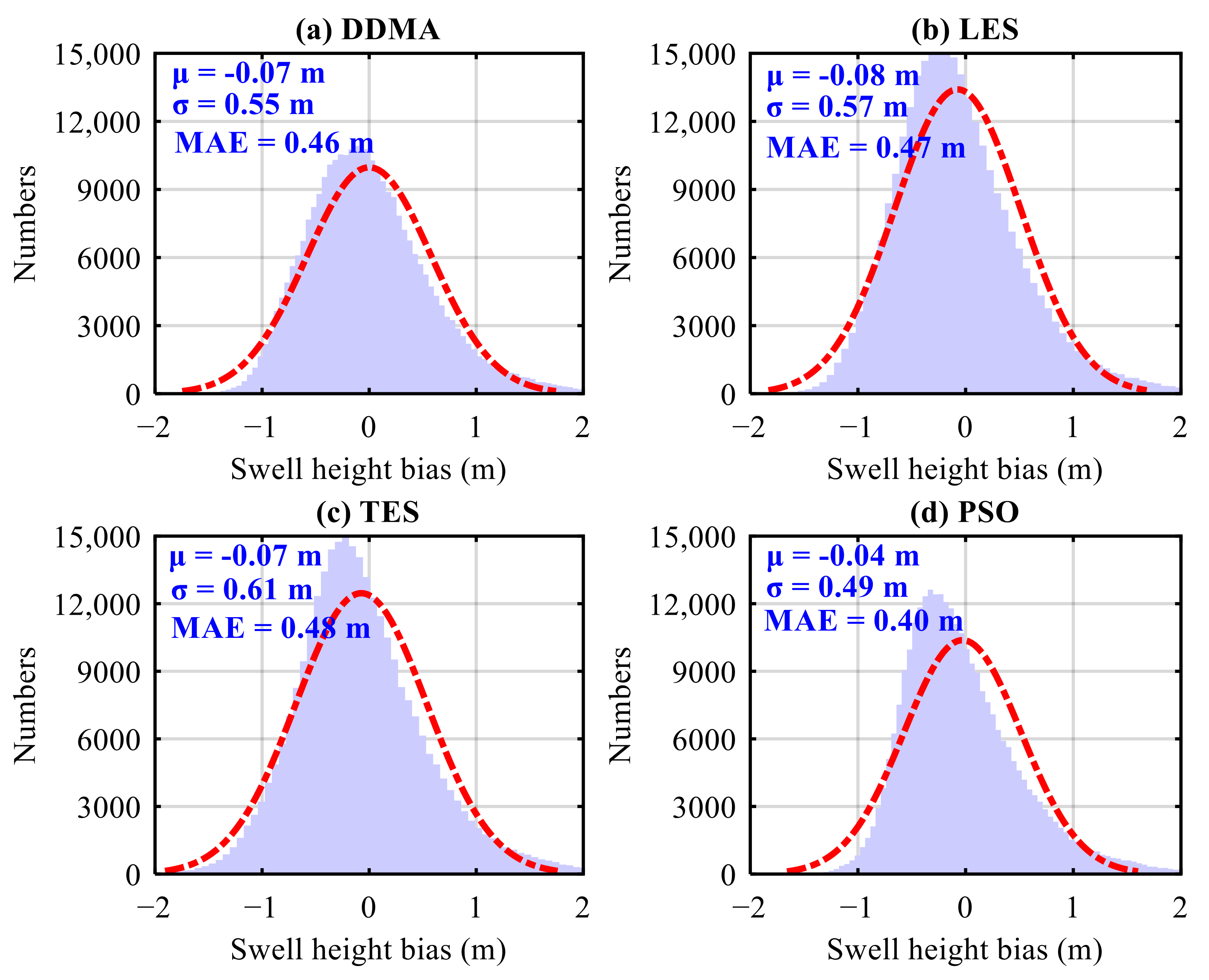
4.1. Performance Evaluation Index

To evaluate the estimation performance of the models, this section compares the swell height estimated by the model with the ERA5 swell height data. RMSE, Pearson correlation coefficient (CC), mean absolute error (MAE), and mean absolute percentage error (MAPE) [27,49] are adopted to evaluate the swell height estimation performance of the models, and they are expressed as follows:

$$RMSE=\sqrt{\frac{1}{m}{\displaystyle \sum _{i=1}^m{(h_{i,E}-h_{i,T})}^2}}$$

(14)

$$MAE=\frac{1}{m}{\displaystyle \sum _{i=1}^m\left|h_{i,E}-h_{i,T}\right|}$$

(15)

$$CC=\frac{{\displaystyle \sum _{i=1}^m(h_{i,E}-\overline{h_E})(h_{i,T}-\overline{h_T})}}{\sqrt{{\displaystyle \sum _{i=1}^m{(h_{i,E}-\overline{h_E})}^2{\displaystyle \sum _{i=1}^m{(h_{i,T}-\overline{h_T})}^2}}}}$$

(16)

$$MAPE=\frac{1}{m}{\displaystyle \sum _{i=1}^m\left|\frac{h_{i,E}-h_{i,T}}{h_{i,T}}\right|}\times 100\%$$

(17)

where $m$ is the number of data samples, $h_{i,E}$ and $h_{i,T}$ are, respectively, the swell height estimated by the model and that obtained from ERA5 reanalysis data, and $\overline{h_E}$ and $\overline{h_T}$ are the average of $h_{i,E}$ and $h_{i,T}$. The details of the performance evaluation are described below.

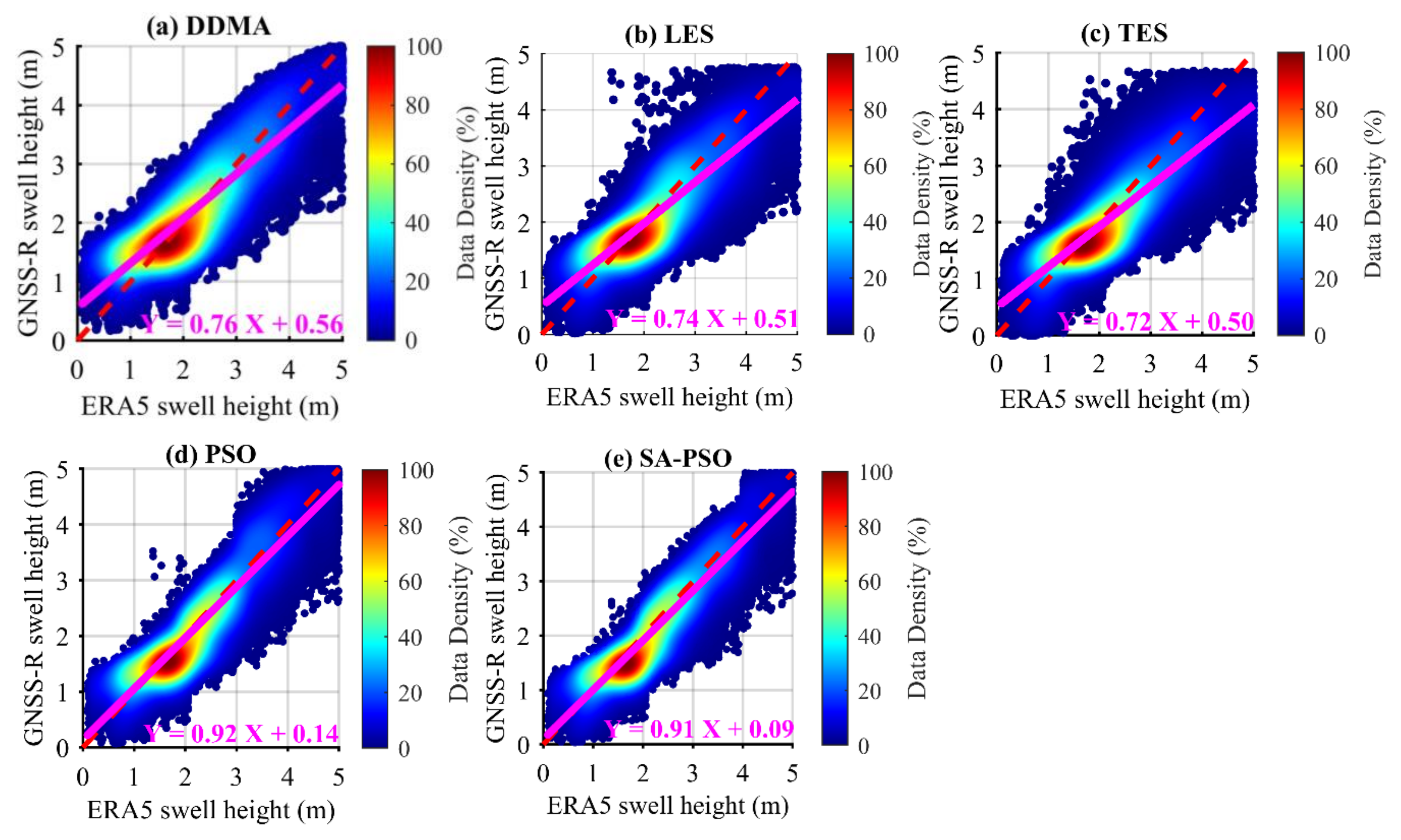
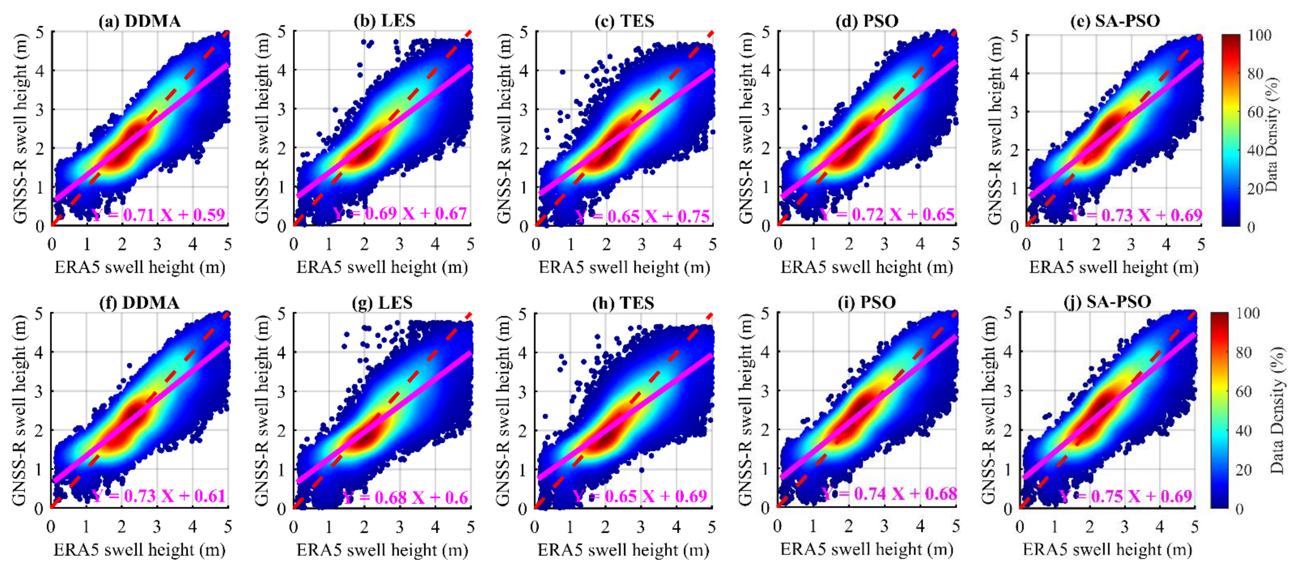
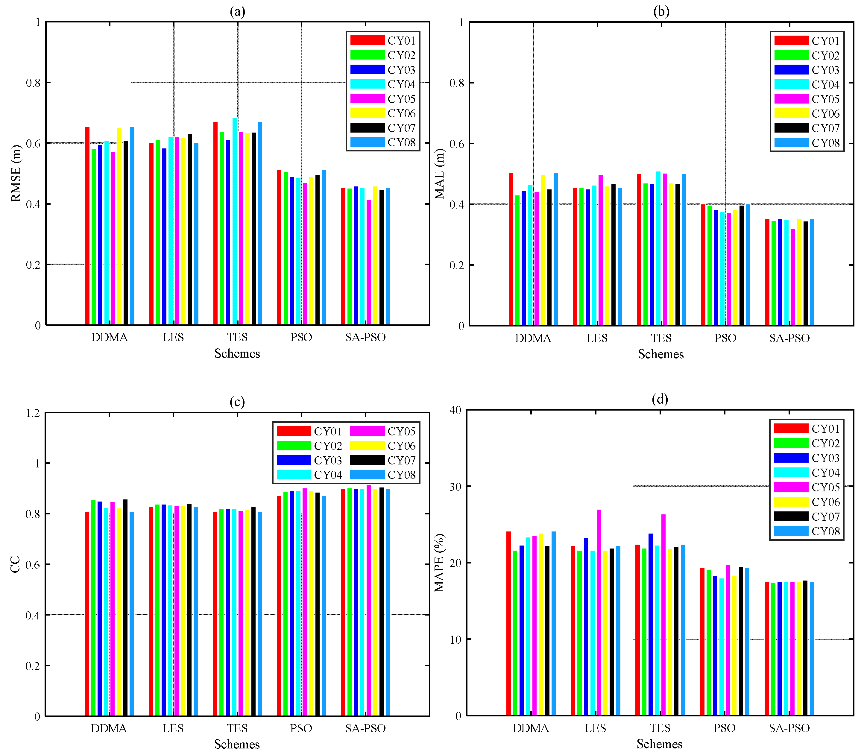
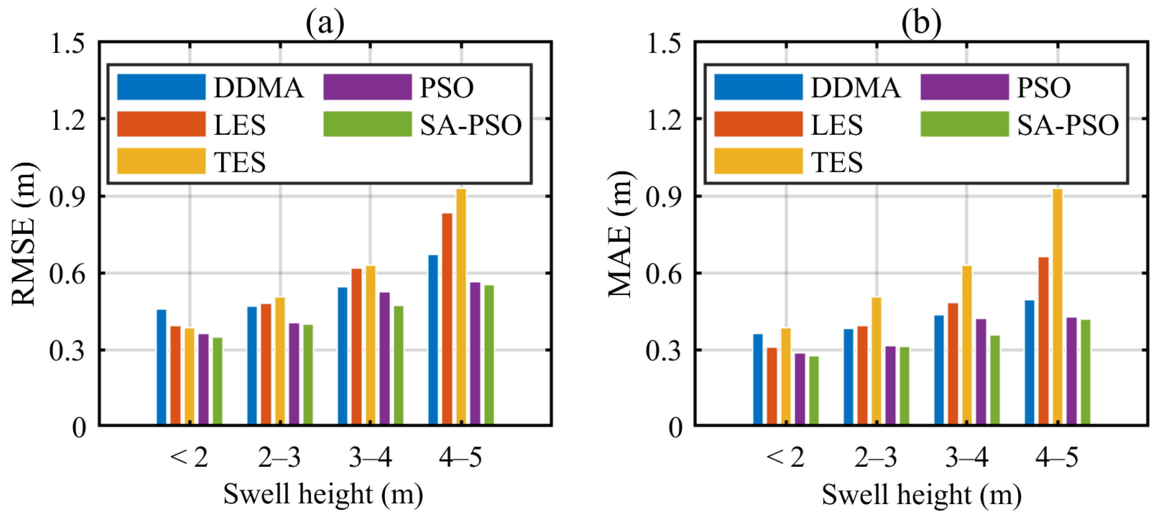
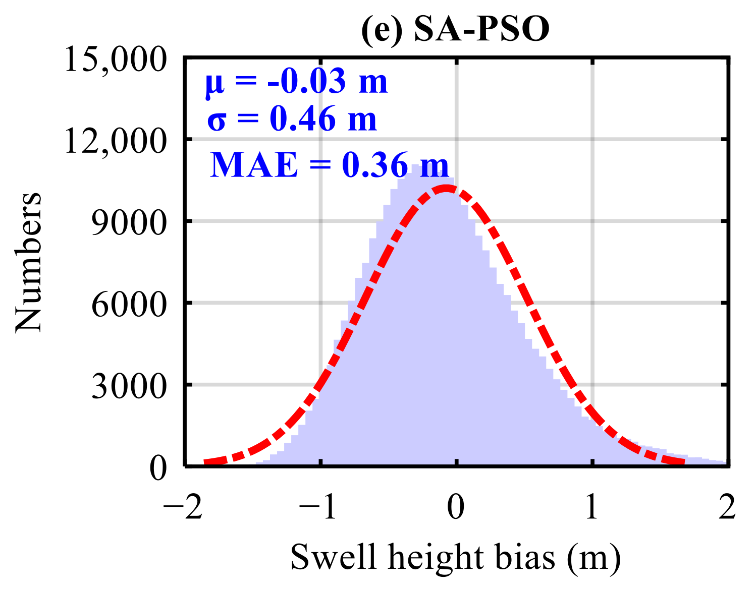
4.2. Results for PSO, SA-PSO, and Other Three Estimates

In this section, we evaluate the swell height estimation performance of five modeling methods. Figure 7 shows the scatter density plots of ERA5 swell height data and that estimated by GNSS-R retrieval model. In the figure, the red dotted line is a 1:1 reference line, the magenta solid line is a linear fitting line ($Y=aX+b$) between GNSS-R results and ERA5 data, and the fitting line equation is also shown in the figure.

Table 1. RMSE, MAE, CC, and MAPE statistics of swell height results retrieved by five schemes.

Methods	RMSE (m)	MAE (m)	CC	MAPE (%)
DDMA	0.51	0.40	0.87	26.04
LES	0.53	0.40	0.87	23.42
TES	0.56	0.42	0.86	22.99
PSO	0.42	0.32	0.91	20.53
SA-PSO	0.39	0.30	0.92	18.98

lists the four retrieval performance evaluation metrics for the five retrieval methods. It can be found from Figure 7 and Table 1 that the swell height retrieved by the five modeling schemes in this study has a good correlation with ERA5 swell height data, and the CC value is better than 0.86. In terms of RMSE, MAE, CC, and MAPE, the retrieval results of the PSO and SA-PSO methods were the best, and the TES observable was the worst. Moreover, compared with DDMA, LES, TES, and PSO, the RMSE of the SA-PSO method was improved by 23.53%, 26.42%, 30.36%, and 7.14%, respectively, the MAE of the SA-PSO method was improved by 25.00%, 25.00%, 28.57%, and 6.25%, respectively, and the MAPE of the SA-PSO method was improved by 27.11%, 18.96, 17.44%, and 7.55%, respectively. In general, the SA-PSO method performed very well.

The error of swell height retrieval is mainly due to two aspects: one is geophysical, the other is the diversity and complexity of the whole CYGNSS system. In order to characterize the deviation between each CYGNSS satellite, we evaluated the swell height estimation performance of each CYGNSS satellite. Due to limited space, Figure 8 only shows the scatter density plots of CY01 and CY02 (from top to bottom) swell height estimates and ERA5 data, respectively (the scatter density plots of CY03-CY08 swell height estimates and ERA5 swell height data are shown in Figures S1–S6 in the Supplementary Materials). Figure 9 shows the statistics of the five retrieval methods for eight CYGNSS satellites.

Table 2. The improvement rates (Unit:%) of the average RMSE, MAE, CC, and MAPE estimated PSO and SA-PSO methods for the swell height of eight CYGNSS satellites compared with DDMA, LES, and TES observables.

	RMSE			MAE			CC			MAPE
Methods	DDMA	LES	TES	DDMA	LES	TES	DDMA	LES	TES	DDMA	LES	TES
PSO	19.57	19.73	24.02	16.80	16.64	20.44	6.25	6.43	8.49	18.70	16.92	17.65
SA-PSO	26.73	26.87	30.78	25.42	25.28	28.68	8.06	8.24	10.34	24.15	22.49	23.17

also illustrates the improvement of the average RMSE, MAE, CC, and MAPE estimated by the PSO and SA-PSO methods for eight CYGNSS satellites compared with the DDMA, LES, and TES observable-based results.

The estimate results for different CYGNSS satellite are approximately the same, as shown in Figure 8 and Figure 9 and Table 2. However, the SA-PSO method outperforms DDMA, LES, TES, and PSO for each CYGNSS satellite. Furthermore, the SA-PSO method is used to retrieve swell height for eight CYGNSS satellites and compared with DDMA, LES, and TES. In terms of the average RMSE, the average improvement rates are 26.73%, 26.87%, and 30.78%, respectively; the average improvement rates of the average MAE are 25.42%, 25.28%, and 28.68%, respectively; the average improvement rates of the average CC are 8.06%, 8.24%, and 10.34%, respectively; and those of the average MAPE are 24.15%, 22.49%, and 23.17%, respectively. The above analysis shows that the SA-PSO method has satisfactory performance for swell height estimation using spaceborne GNSS-R data. Such improvements also highlight that the SA-PSO method has significant potential to improve the retrieval accuracy obtained using a single observable.

4.3. Discussion

It is necessary to evaluate the applicability of each model to estimate swell height under different sea states. Figure 10 shows the RMSE and MAE of swell height estimates by the DDMA, LES, TES, PSO, and SA-PSO methods under different sea states. The results show that the retrieval error of a single observable-based method is large under the condition of high swell height. However, the retrieval performances of the PSO and SA-PSO methods are both better than that of a single observable-based method under different sea conditions. In addition, we can see that the retrieval accuracy decreases when swell height increases. Therefore, the swell height estimation performance for a high sea state needs to be further improved.

We also evaluated the global performance of swell height estimated by different retrieval methods. Figure 11 shows the global distribution of the GNSS-R swell height and ERA5 data in June and July 2019. It can be seen that the CYGNSS result is consistent with ERA5 in general. Large swell height values are seen mostly in high latitudes, particularly in the South. This indicates that swell is dominant in high latitudes and there is a phenomenon of swell intensification. Usually, swell is transmitted from other sea areas on the sea surface, or the local wind force rapidly decreases and subsides, or the wave left on the sea surface after the wind direction changes. The wave surface of a swell is relatively flat and smooth, with a long wave peak line and large period and wavelength. As mentioned previously, the coverage of the CYGNSS tracks is limited, current CYGNSS observation data cannot be used to estimate the swell height around the Arctic Ocean or Antarctica. For future research, we can consider combining TDS-1 or other satellite observation data to obtain swell height results around the Arctic Ocean or Antarctica. Figure 12 shows the PDFs of swell height retrieved by different methods and ERA5 swell height.

Table 3. Mean and standard deviation of swell height estimated by different methods.

	ERA5	DDMA	LES	TES	PSO	SA-PSO
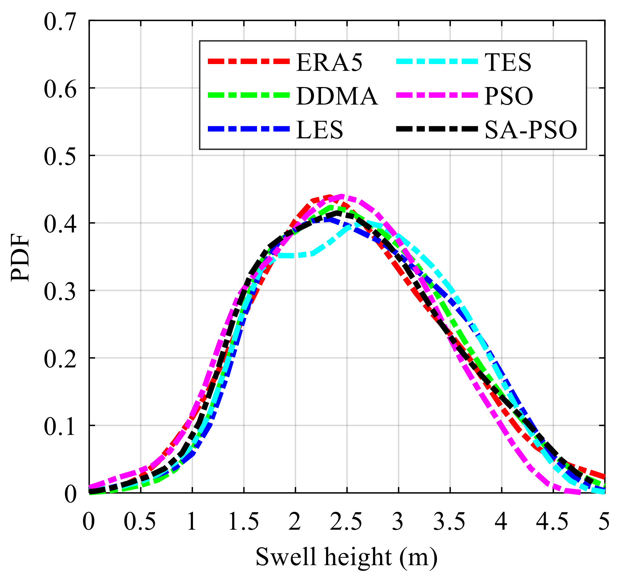
Mean swell height (m)	2.61	2.60	2.68	2.69	2.68	2.63
Standard deviation (m)	0.88	0.85	0.87	0.87	0.86	0.82

shows the mean and standard deviation of swell height estimated by different methods. It can be seen from Figure 12 and Table 3 that the mean swell height of ERA5 data is 2.61 m; the mean swell heights by DDMA, LES, TES, PSO, and SA-PSO are 2.60 m, 2.69 m, 2.68 m, 2.68 m, and 2.63 m, respectively. The standard deviation of ERA5 swell height data is 0.88 m; the standard deviations obtained by DDMA, LES, TES, PSO, and SA-PSO are 0.85 m, 0.87 m, 0.87 m, 0.86 m, 0.82 m, respectively. In general, the swell heights estimated by the five methods are in good agreement with the ERA5 data.

To compare the global error distribution of different methods, Figure 13 depicts the deviation distribution histogram between GNSS-R retrieved swell height and ERA5 data on a global scale for June and July 2019. In the figure, the mean deviation (μ), standard deviation (σ), and mean absolute error (MAE) are also given. The light blue bar graph indicates the error distribution, and the red dotted line represents the PDFs fitting curve of the error. It is found that the deviation of swell height retrieved by the GNSS-R based methods are approximately normally distributed. The mean deviation, standard deviation, and mean absolute error between swell height retrieved by the five methods and ERA5 swell height are better than −0.08 m, 0.61 m, and 0.48 m, respectively. Among the five methods, the LES method is worse than other methods. Furthermore, the positive deviation mainly occurs in high latitudes of the northern and southern hemispheres, particularly in the southern hemisphere. When the latitude exceeds 30°S, the deviation is obvious. Overall, the swell height results observed by CYGNSS measurements are fundamentally consistent with those of the ERA5 products. The accuracy of swell height retrieval is basically satisfactory, which shows the feasibility of the proposed method.

As described in [50], swell has a significant input of more than 75% into SWH for mixed waves. Therefore, it is interesting to calculate CC, RMSE, MAE, and MAPE for the following two cases: (a) swell height estimated from spaceborne CNSS-R (i.e., the SA-PSO method) vs. ERA5 swell height; (b) swell height estimated from spaceborne CNSS-R (i.e., the SA-PSO method) vs. ERA5 SWH (Hs).

Table 4. RMSE, MAE, CC, and MAPE statistics by comparing the swell height results retrieved using the SA-PSO method with ERA5 swell height and ERA5 SWH (Hs).

	SA-PSO Method Swell Height vs. ERA5 Swell Height				SA-PSO Method Swell Height vs. ERA5 SWH (Hs)
	RMSE (m)	MAE (m)	CC	MAPE (%)	RMSE (m)	MAE (m)	CC	MAPE (%)
CY01	0.45	0.35	0.89	17.57	0.70	0.51	0.72	30.97
CY02	0.45	0.35	0.90	17.44	0.71	0.52	0.72	31.54
CY03	0.45	0.35	0.90	17.43	0.67	0.51	0.73	31.11
CY04	0.45	0.35	0.90	17.44	0.69	0.52	0.72	31.48
CY05	0.41	0.32	0.91	17.56	0.67	0.51	0.73	31.33
CY06	0.46	0.35	0.90	17.58	0.72	0.53	0.70	31.76
CY07	0.45	0.34	0.90	17.72	0.69	0.51	0.73	31.14
CY08	0.45	0.35	0.89	17.57	0.68	0.51	0.72	30.68
Eight CYGNSS	0.39	0.30	0.92	18.98	0.58	0.40	0.81	25.17

shows the RMSE, MAE, CC, and MAPE statistics by comparing the swell height results retrieved from CYGNSS satellite data using the SA-PSO method with ERA5 swell height and ERA5 SWH (Hs). It can be seen from Table 4 that although the swell height estimated by the proposed SA-PSO method has a certain correlation with the mixed waves, it is more consistent with the ERA5 swell height. The performed comparison suggests that global swell height can be estimated from GNSS-R data with the use of the proposed method.

It is worth mentioning that other wave parameters are also important. This research is an early attempt with the spaceborne GNSS-R technology for swell parameters retrieval although the experiments were not dedicated for this research. The focus of this study is to propose an empirical model for retrieving swell height from spaceborne GNSS-R data. In addition, it is very challenging to consider so many sea state parameters based on the empirical model method. One possible solution is to use machine- or deep-learning-based methods. This will be an important topic of future spaceborne GNSS-R sea state monitoring research.

5. Conclusions

This research developed an empirical model for swell height retrieval utilizing three GNSS-R observables (i.e., DDMA, LES, and TES) derived from spaceborne GNSS-R data. To improve the retrieval performance of individual observables, the PSO method is first introduced. Moreover, to solve the local optimal solution of the PSO algorithm, a SA-PSO algorithm is proposed. To demonstrate the validation of the proposed models, the ERA5 swell height data are employed to compare and verify the swell height estimation results based on the proposed five schemes. Among them, the best performance was obtained based on the SA-PSO method, and compared with DDMA, LES, TES, and PSO, the RMSE of the SA-PSO method was improved by 23.53%, 26.42%, 30.36%, and 7.14%, respectively; the MAE of SA-PSO method was improved by 25.00%, 25.00%, 28.57%, and 6.25%, respectively, and the MAPE of SA-PSO method was improved by 27.11%, 18.96, 17.44%, and 7.55%, respectively. In general, the SA-PSO method achieved a good performance. Furthermore, the global swell height estimation results also showed that the CYGNSS swell height estimation and the ERA5 data were consistent. It further confirmed the validation of the proposed method in this study.

In the future, more data will be exploited to show the feasibility of swell height estimation. Meanwhile, we will investigate swell height estimation under high sea states. Additionally, multi-frequency and multi-GNSS reflected signals will be exploited for swell height estimation to further improve the retrieval performance. Finally, we also encourage estimating as many ocean parameters (e.g., wave period and wave direction) as possible, which is very useful for oceanographic applications. For example, Reinking et al. [51] used cut-off elevation to estimate wave direction based on terrestrial GNSS-R data, and Wang et al. [52] used GNSS interferometry reflectometry (GNSS-IR) to estimate the wave peak period. However, for most spaceborne cases, this technology is not yet mature. This study is an early attempt with the spaceborne GNSS-R technology for swell parameter (here swell height) retrieval. Whether the spaceborne GNSS-R technology can be used to estimate the wave direction and wave period needs further investigation, which will also be an important topic of future spaceborne GNSS-R sea state monitoring research.

References

- Wang, W.; Forget, P.; Guan, C. Inversion and assessment of swell waveheights from HF radar spectra in the Iroise Sea. Ocean Dyn. 2016, 66, 527–538. [Google Scholar] [CrossRef]
- Albuquerque, J.; Antolínez, J.A.; Rueda, A.; Méndez, F.J.; Coco, G. Directional correction of modeled sea and swell wave heights using satellite altimeter data. Ocean Model. 2018, 131, 103–114. [Google Scholar] [CrossRef]
- Mognard, N.M. Swell in the Pacific Ocean observed by SEASAT radar altimeter. Mar. Geodesy 1984, 8, 183–210. [Google Scholar] [CrossRef]
- Mognard, N.M.; Campbell, W.J.; Brossier, C. World Ocean mean monthly waves, swell, and surface winds for July through October 1978 from SEASAT radar altimeter data. Mar. Geodesy 1984, 8, 159–181. [Google Scholar] [CrossRef]
- Li, X.M. A new insight from space into swell propagation and crossing in the global oceans. Geophys. Res. Lett. 2016, 43, 5202–5209. [Google Scholar] [CrossRef]
- Altiparmaki, O.; Kleinherenbrink, M.; Naeije, M.; Slobbe, C.; Visser, P. SAR Altimetry Data as a New Source for Swell Monitoring. Geophys. Res. Lett. 2022, 49, e2021GL096224. [Google Scholar] [CrossRef]
- Wang, H.; Mouche, A.; Husson, R.; Chapron, B. Indian Ocean Crossing Swells: New Insights from “Fireworks” Perspective Using Envisat Advanced Synthetic Aperture Radar. Remote Sens. 2021, 13, 670. [Google Scholar] [CrossRef]
- Wang, H.; Mouche, A.; Husson, R.; Grouazel, A.; Chapron, B.; Yang, J. Assessment of Ocean Swell Height Observations from Sentinel-1A/B Wave Mode against Buoy in Situ and Modeling Hindcasts. Remote Sens. 2022, 14, 862. [Google Scholar] [CrossRef]
- Wang, H.; Mouche, A.; Husson, R.; Chapron, B. Dynamic validation of ocean swell derived from Sentinel-1 wave mode against buoys. In Proceedings of the IGARSS 2018—2018 IEEE International Geoscience and Remote Sensing Symposium, Valencia, Spain, 22–27 July 2018; pp. 3223–3226. [Google Scholar]
- Ardhuin, F.; Rogers, E.; Babanin, A.V.; Filipot, J.-F.; Magne, R.; Roland, A.; Van Der Westhuysen, A.; Queffeulou, P.; Lefevre, J.-M.; Aouf, L.; et al. Semiempirical Dissipation Source Functions for Ocean Waves. Part I: Definition, Calibration, and Validation. J. Phys. Oceanogr. 2010, 40, 1917–1941. [Google Scholar] [CrossRef]
- Lipa, B.; Barrick, D. Methods for the extraction of long-period ocean wave parameters from narrow beam HF radar sea echo. Radio Sci. 1980, 15, 843–853. [Google Scholar] [CrossRef]
- Lipa, B.J.; Barrick, D.E.; Maresca, J.W., Jr. HF radar measurements of long ocean waves. J. Geophys. Res. Oceans 1981, 86, 4089–4102. [Google Scholar] [CrossRef]
- Bathgate, J.S.; Heron, M.L.; Prytz, A. A Method of Swell-Wave Parameter Extraction from HF Ocean Surface Radar Spectra. IEEE J. Ocean. Eng. 2006, 31, 812–818. [Google Scholar] [CrossRef]
- Shen, C.; Gill, E.; Huang, W. Extraction of swell parameters from simulated noisy HF radar signals. In Proceedings of the 2013 IEEE Radar Conference (RadarCon13), Ottawa, ON, Canada, 29 April–3 May 2013; pp. 1–6. [Google Scholar] [CrossRef]
- Alattabi, Z.R.; Cahl, D.; Voulgaris, G. Swell and Wind Wave Inversion Using a Single Very High Frequency (VHF) Radar. J. Atmos. Ocean. Technol. 2019, 36, 987–1013. [Google Scholar] [CrossRef]
- Al-Attabi, Z.R.; Voulgaris, G.; Conley, D.C. Evaluation and Validation of HF Radar Swell and Wind wave Inversion Method. J. Atmos. Ocean. Technol. 2021, 38, 1747–1775. [Google Scholar] [CrossRef]
- Liu, X.; Huang, W.; Gill, E.W. Estimation of Significant Wave Height From X-Band Marine Radar Images Based on Ensemble Empirical Mode Decomposition. IEEE Geosci. Remote Sens. Lett. 2017, 14, 1740–1744. [Google Scholar] [CrossRef]
- Liu, X.; Huang, W.; Gill, E.W. Wave Height Estimation from Shipborne X-Band Nautical Radar Images. J. Sens. 2016, 2016, 1078053. [Google Scholar] [CrossRef]
- Wu, L.-C.; Doong, D.-J.; Lai, J.-W. Influences of Nononshore Winds on Significant Wave Height Estimations Using Coastal X-Band Radar Images. IEEE Trans. Geosci. Remote Sens. 2021, 60, 4202111. [Google Scholar] [CrossRef]
- Huang, W.; Liu, X.; Gill, E.W. Ocean Wind and Wave Measurements Using X-Band Marine Radar: A Comprehensive Review. Remote Sens. 2017, 9, 1261. [Google Scholar] [CrossRef]
- Hammond, M.L.; Foti, G.; Gommenginger, C.; Srokosz, M. Temporal variability of GNSS-Reflectometry Ocean wind speed retrieval performance during the UK TechDemoSat-1 mission. Remote Sens. Environ. 2020, 242, 111744. [Google Scholar] [CrossRef]
- Clarizia, M.P.; Ruf, C.S. Bayesian Wind Speed Estimation Conditioned on Significant Wave Height for GNSS-R Ocean Observations. J. Atmos. Ocean. Technol. 2017, 34, 1193–1202. [Google Scholar] [CrossRef]
- Li, W.; Rius, A.; Fabra, F.; Cardellach, E.; Ribo, S.; Martin-Neira, M. Revisiting the GNSS-R Waveform Statistics and Its Impact on Altimetric Retrievals. IEEE Trans. Geosci. Remote Sens. 2018, 56, 2854–2871. [Google Scholar] [CrossRef]
- Yan, Q.; Huang, W. Spaceborne GNSS-R Sea Ice Detection Using Delay-Doppler Maps: First Results from the U.K. TechDemoSat-1 Mission. IEEE J. Sel. Top. Appl. Earth Obs. Remote Sens. 2016, 9, 4795–4801. [Google Scholar] [CrossRef]
- Yu, K. Weak Tsunami Detection Using GNSS-R-Based Sea Surface Height Measurement. IEEE Trans. Geosci. Remote Sens. 2016, 54, 1363–1375. [Google Scholar] [CrossRef]
- Asgarimehr, M.; Zavorotny, V.U.; Wickert, J.; Reich, S. Can GNSS Reflectometry Detect Precipitation Over Oceans? Geophys. Res. Lett. 2018, 45, 12585–12592. [Google Scholar] [CrossRef]
- Bu, J.; Yu, K. Sea Surface Rainfall Detection and Intensity Retrieval Based on GNSS-Reflectometry Data From the CYGNSS Mission. IEEE Trans. Geosci. Remote Sens. 2022, 60, 5802015. [Google Scholar] [CrossRef]
- Bu, J.; Yu, K.; Han, S.; Qian, N.; Lin, Y.; Wang, J. Retrieval of Sea Surface Rainfall Intensity Using Spaceborne GNSS-R Data. IEEE Trans. Geosci. Remote Sens. 2022, 60, 5803116. [Google Scholar] [CrossRef]
- Bu, J.; Yu, K.; Ni, J.; Yan, Q.; Han, S.; Wang, J.; Wang, C. Machine learning-based methods for sea surface rainfall detection from CYGNSS delay-doppler maps. GPS Solut. 2022, 26, 132. [Google Scholar] [CrossRef]
- Foti, G.; Gommenginger, C.; Jales, P.; Unwin, M.; Shaw, A.; Robertson, C.; Roselló, J. Spaceborne GNSS reflectometry for ocean winds: First results from the UK TechDemoSat-1 mission. Geophys. Res. Lett. 2015, 42, 5435–5441. [Google Scholar] [CrossRef]
- Clarizia, M.P.; Ruf, C.S. Wind Speed Retrieval Algorithm for the Cyclone Global Navigation Satellite System (CYGNSS) Mission. IEEE Trans. Geosci. Remote Sens. 2016, 54, 4419–4432. [Google Scholar] [CrossRef]
- Jing, C.; Niu, X.; Duan, C.; Lu, F.; Di, G.; Yang, X. Sea Surface Wind Speed Retrieval from the First Chinese GNSS-R Mission: Technique and Preliminary Results. Remote Sens. 2019, 11, 3013. [Google Scholar] [CrossRef]
- Munoz-Martin, J.F.; Fernandez, L.; Perez, A.; Ruiz-De-Azua, J.A.; Park, H.; Camps, A.; Domínguez, B.C.; Pastena, M. In-Orbit Validation of the FMPL-2 Instrument—The GNSS-R and L-Band Microwave Radiometer Payload of the FSSCat Mission. Remote Sens. 2021, 13, 121. [Google Scholar] [CrossRef]
- Yang, G.; Bai, W.; Wang, J.; Hu, X.; Zhang, P.; Sun, Y.; Xu, N.; Zhai, X.; Xiao, X.; Xia, J.; et al. FY3E GNOS II GNSS Reflectometry: Mission Review and First Results. Remote Sens. 2022, 14, 988. [Google Scholar] [CrossRef]
- Peng, Q.; Jin, S. Significant Wave Height Estimation from Space-Borne Cyclone-GNSS Reflectometry. Remote Sens. 2019, 11, 584. [Google Scholar] [CrossRef]
- Yang, S.; Jin, S.; Jia, Y.; Ye, M. Significant Wave Height Estimation from Joint CYGNSS DDMA and LES Observations. Sensors 2021, 21, 6123. [Google Scholar] [CrossRef]
- Bu, J.; Yu, K. Significant Wave Height Retrieval Method Based on Spaceborne GNSS Reflectometry. IEEE Geosci. Remote Sens. Lett. 2022, 19, 1503705. [Google Scholar] [CrossRef]
- Bu, J.; Yu, K. A New Integrated Method of CYGNSS DDMA and LES Measurements for Significant Wave Height estimation. IEEE Geosci. Remote Sens. Lett. 2022, 19, 1505605. [Google Scholar] [CrossRef]
- Wang, F.; Yang, D.; Yang, L. Retrieval and Assessment of Significant Wave Height from CYGNSS Mission Using Neural Network. Remote Sens. 2022, 14, 3666. [Google Scholar] [CrossRef]
- Yu, K.; Han, S.; Bu, J.; An, Y.; Zhou, Z.; Wang, C.; Tabibi, S.; Cheong, J.W. Spaceborne GNSS Reflectometry. Remote Sens. 2022, 14, 1605. [Google Scholar] [CrossRef]
- Hwang, P.A.; Ocampo-Torres, F.; Nava, H.G. Wind Sea and Swell Separation of 1D Wave Spectrum by a Spectrum Integration Method. J. Atmos. Ocean. Technol. 2012, 29, 116–128. [Google Scholar] [CrossRef]
- Guo, W.; Du, H.; Cheong, J.W.; Southwell, B.J.; Dempster, A.G. GNSS-R Wind Speed Retrieval of Sea Surface Based on Particle Swarm Optimization Algorithm. IEEE Trans. Geosci. Remote Sens. 2021, 60, 4202414. [Google Scholar] [CrossRef]
- Ruf, C.S.; Balasubramaniam, R. Development of the CYGNSS Geophysical Model Function for Wind Speed. IEEE J. Sel. Top. Appl. Earth Obs. Remote Sens. 2019, 12, 66–77. [Google Scholar] [CrossRef]
- Asgarimehr, M.; Arnold, C.; Weigel, T.; Ruf, C.; Wickert, J. GNSS reflectometry global ocean wind speed using deep learning: Development and assessment of CyGNSSnet. Remote Sens. Environ. 2022, 269, 112801. [Google Scholar] [CrossRef]
- Zavorotny, V.; Voronovich, A. Scattering of GPS signals from the ocean with wind remote sensing application. IEEE Trans. Geosci. Remote Sens. 2000, 38, 951–964. [Google Scholar] [CrossRef]
- Clarizia, M.P.; Ruf, C.S.; Jales, P.; Gommenginger, C. Spaceborne GNSS-R Minimum Variance Wind Speed Estimator. IEEE Trans. Geosci. Remote Sens. 2014, 52, 6829–6843. [Google Scholar] [CrossRef]
- Rodriguez-Alvarez, N.; Holt, B.; Jaruwatanadilok, S.; Podest, E.; Cavanaugh, K.C. An Arctic Sea ice multi-step classification based on GNSS-R data from the TDS-1 mission. Remote Sens. Environ. 2019, 230, 111202. [Google Scholar] [CrossRef]
- Camps, A.; Park, H.; Pablos, M.; Foti, G.; Gommenginger, C.P.; Liu, P.-W.; Judge, J. Sensitivity of GNSS-R Spaceborne Observations to Soil Moisture and Vegetation. IEEE J. Sel. Top. Appl. Earth Obs. Remote Sens. 2016, 9, 4730–4742. [Google Scholar] [CrossRef]
- Bu, J.; Yu, K.; Zhu, Y.; Qian, N.; Chang, J. Developing and Testing Models for Sea Surface Wind Speed Estimation with GNSS-R Delay Doppler Maps and Delay Waveforms. Remote Sens. 2020, 12, 3760. [Google Scholar] [CrossRef]
- Semedo, A.; Suselj, K.; Rutgersson, A.; Sterl, A. A Global View on the Wind Sea and Swell Climate and Variability from ERA-40. J. Clim. 2011, 24, 1461–1479. [Google Scholar] [CrossRef]
- Reinking, J.; Roggenbuck, O.; Even-Tzur, G. Estimating Wave Direction Using Terrestrial GNSS Reflectometry. Remote Sens. 2019, 11, 1027. [Google Scholar] [CrossRef] [Green Version]
- Wang, X.; He, X.; Shi, J.; Chen, S.; Niu, Z. Estimating Sea level, wind direction, significant wave height, and wave peak period using a geodetic GNSS receiver. Remote Sens. Environ. 2022, 279, 113135. [Google Scholar] [CrossRef]