
A Novel Multi-Candidate Multi-Correlation Coefficient Algorithm for GOCI-Derived Sea-Surface Current Vector with OSU Tidal Model
Abstract
:1. Introduction
2. Data Set
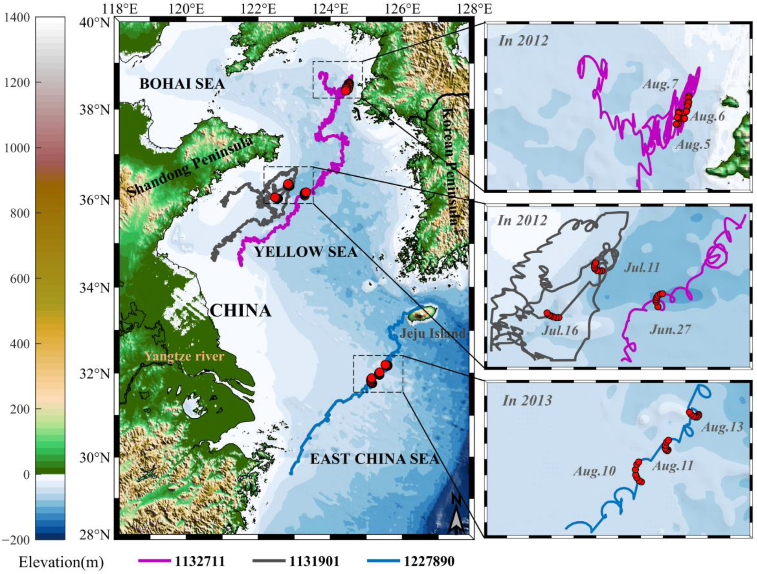
2.1. In-Situ Data
2.2. GOCI Data
2.3. OSU Tidal Current Model Data
3. Methodology
3.1. GOCI Data Processing
3.2. Drifting Buoy Data Processing
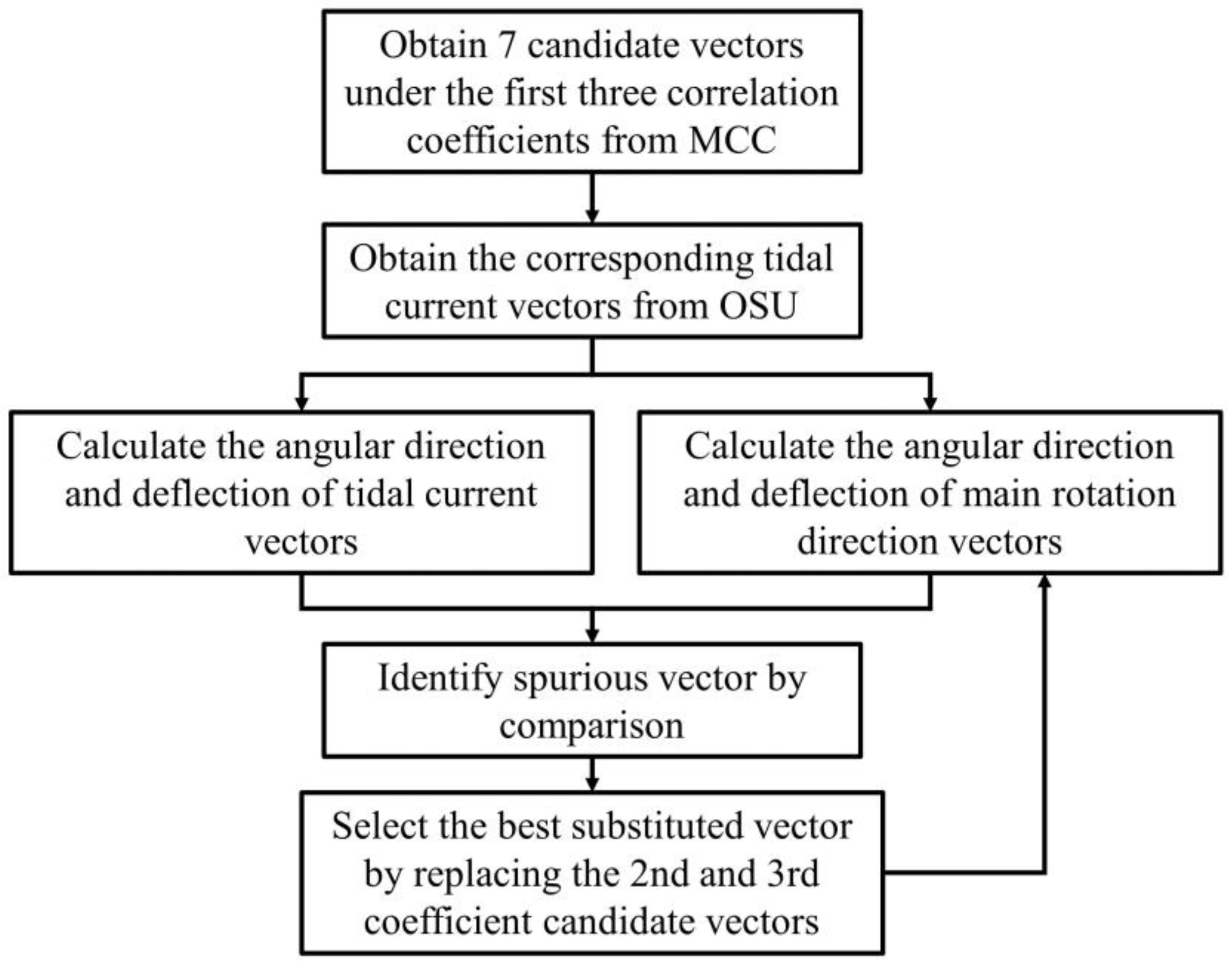
3.3. Multi-Candidate Multi-Correlation Coefficient Optimization Algorithm
3.4. Evaluation Method
4. Results
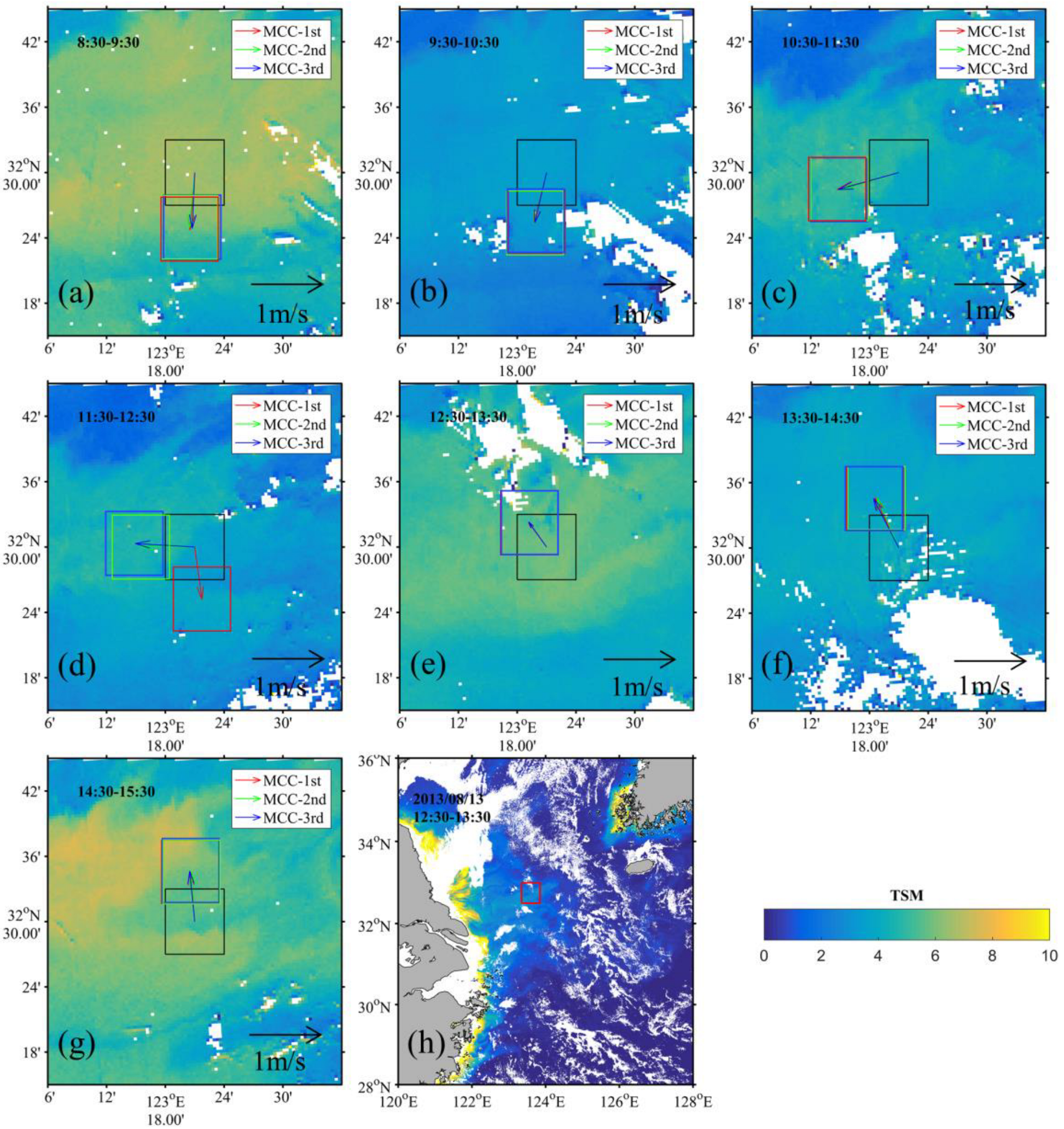
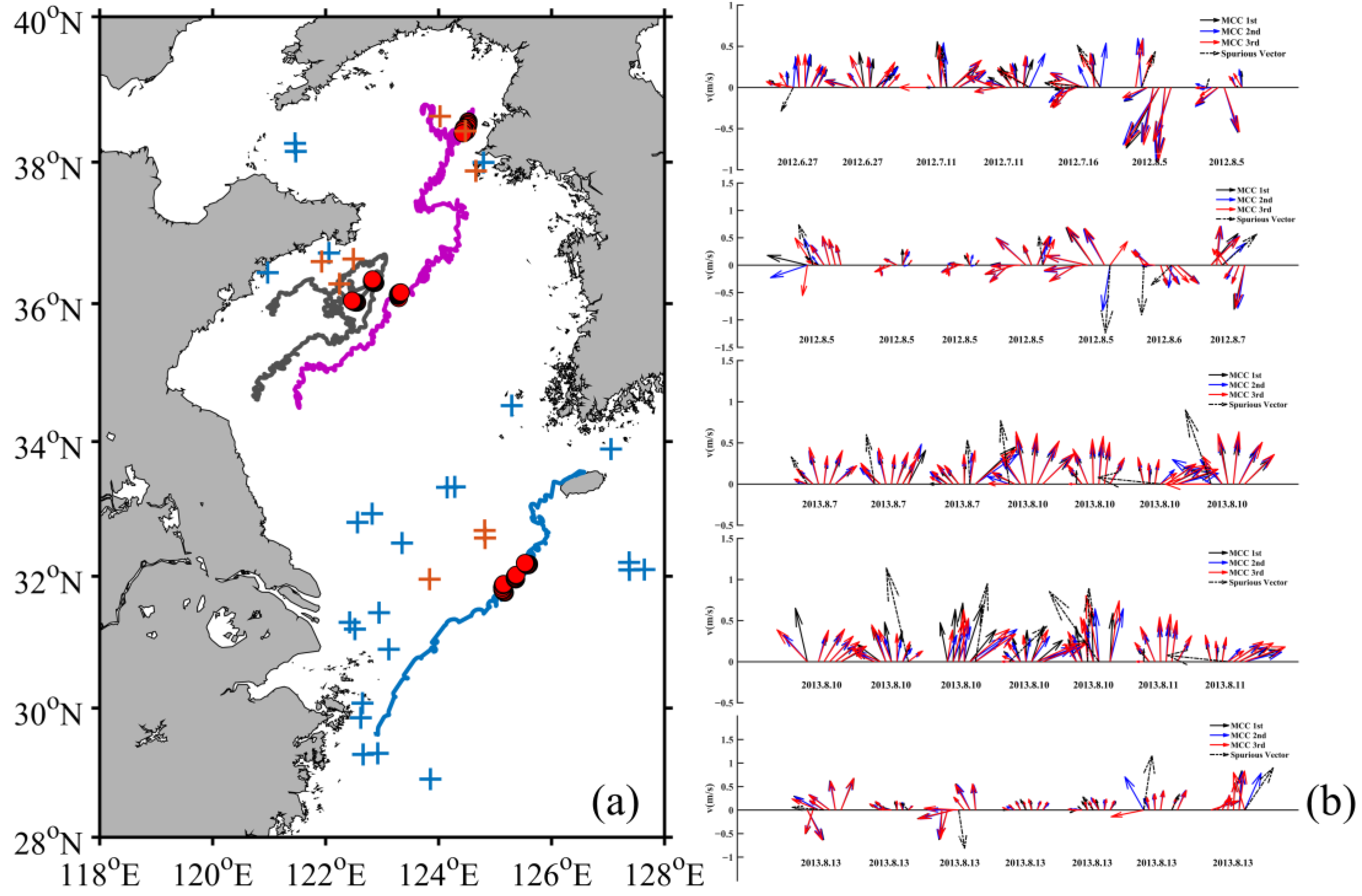
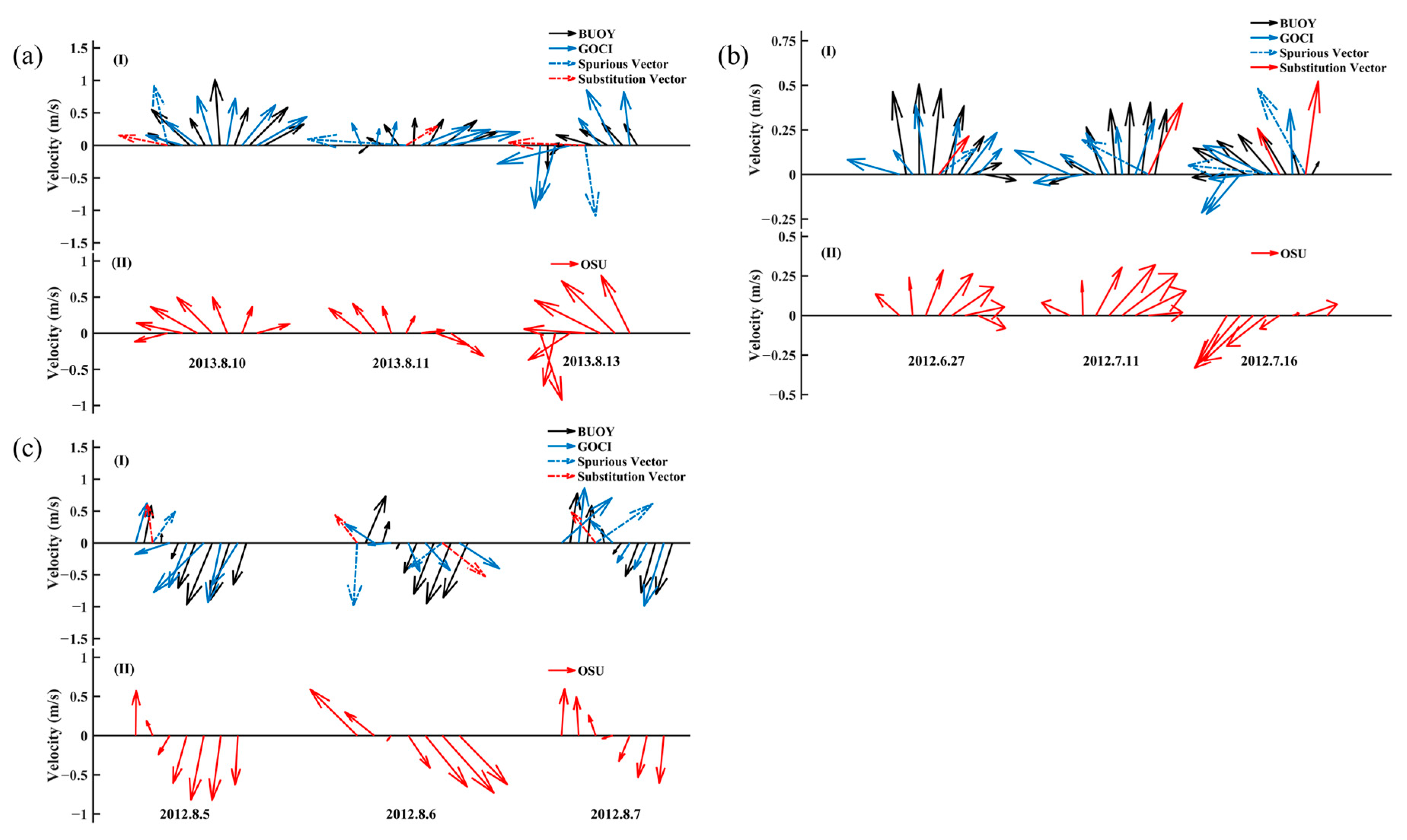
4.1. Vector Processing Results Based on the Multi-Correlation Coefficient Algorithm
4.2. Average Magnitude and Angular Error
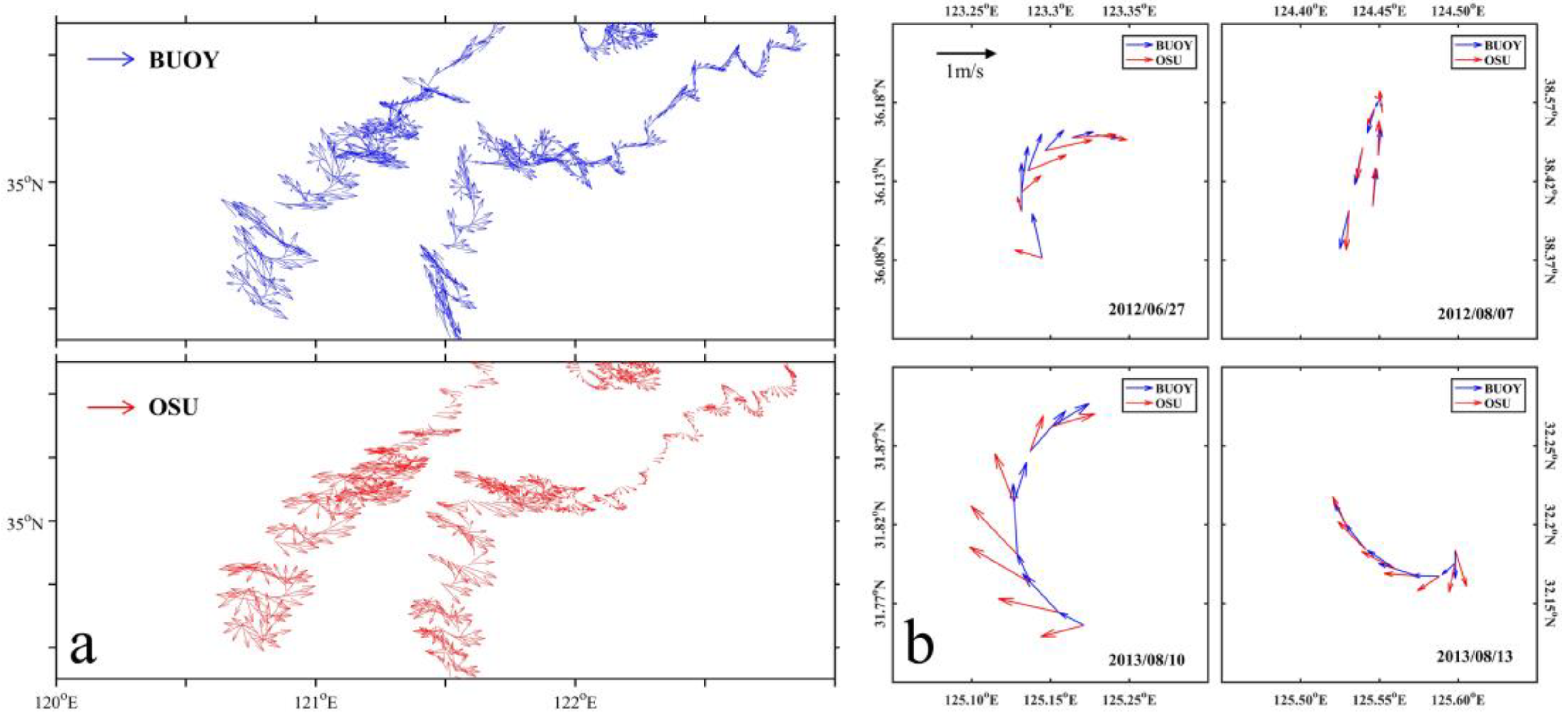
4.3. OSU Tidal Model Data Evaluation
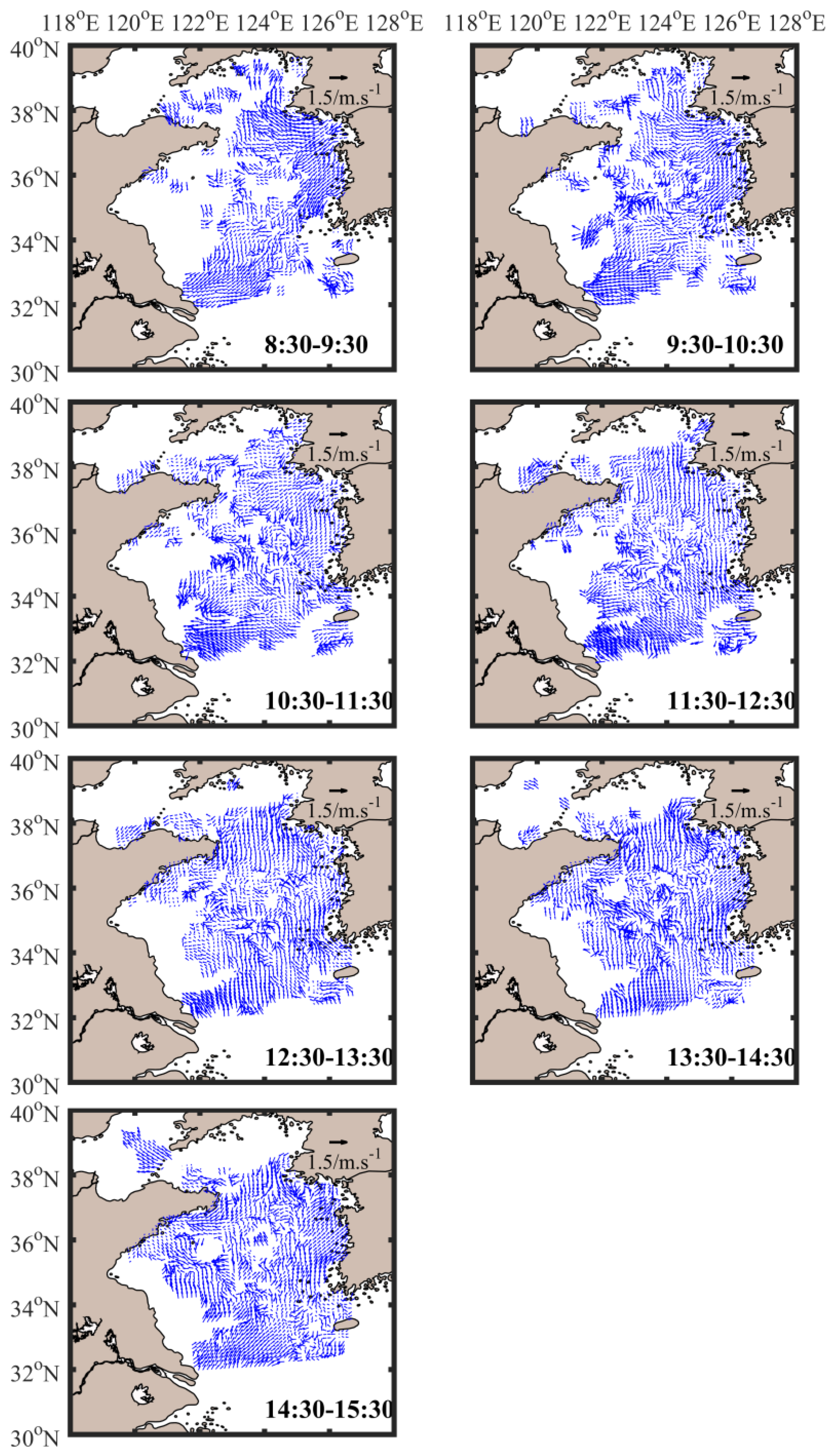
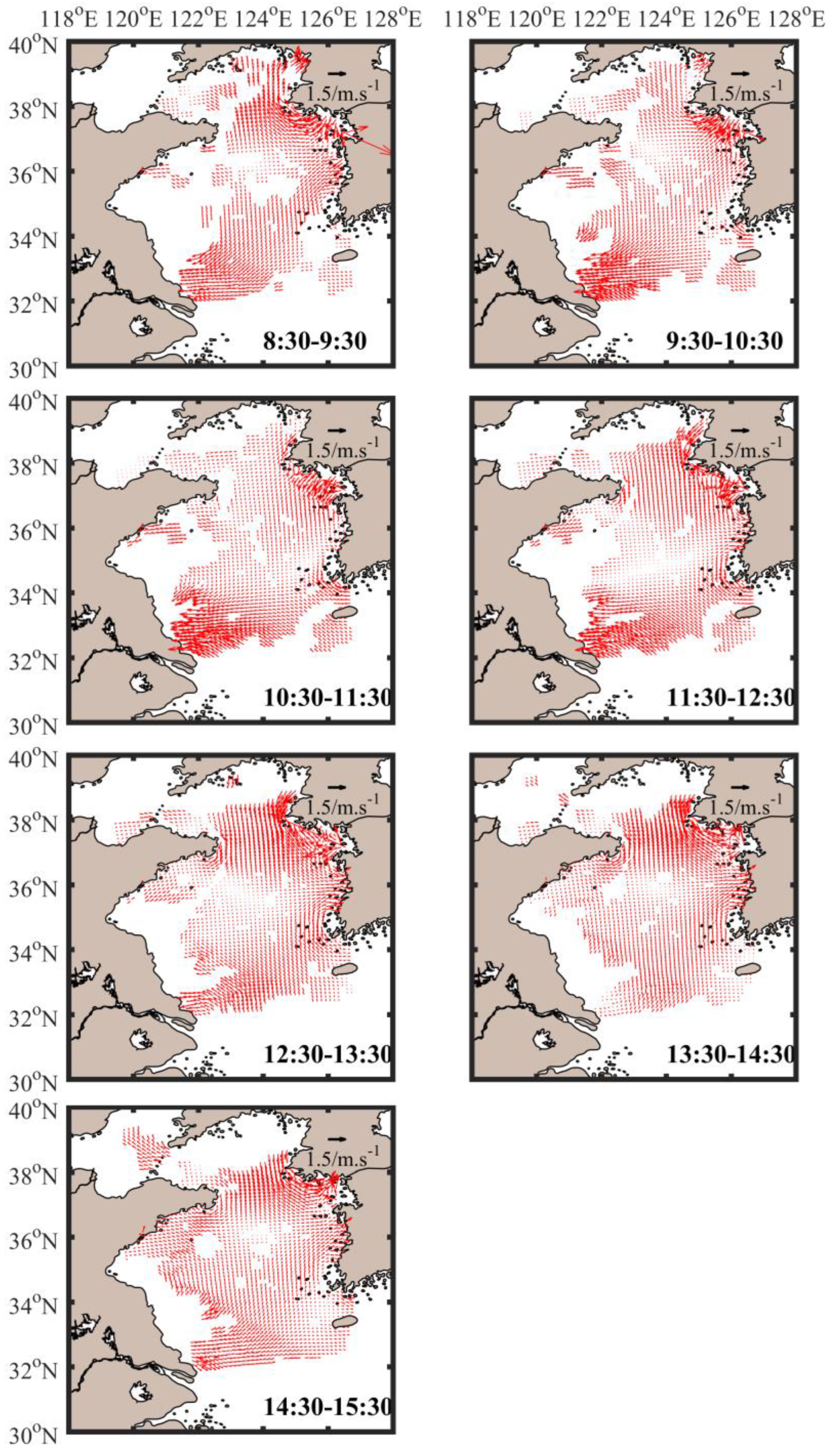
4.4. SSC Mapping from GOCI and OSU
5. Discussion
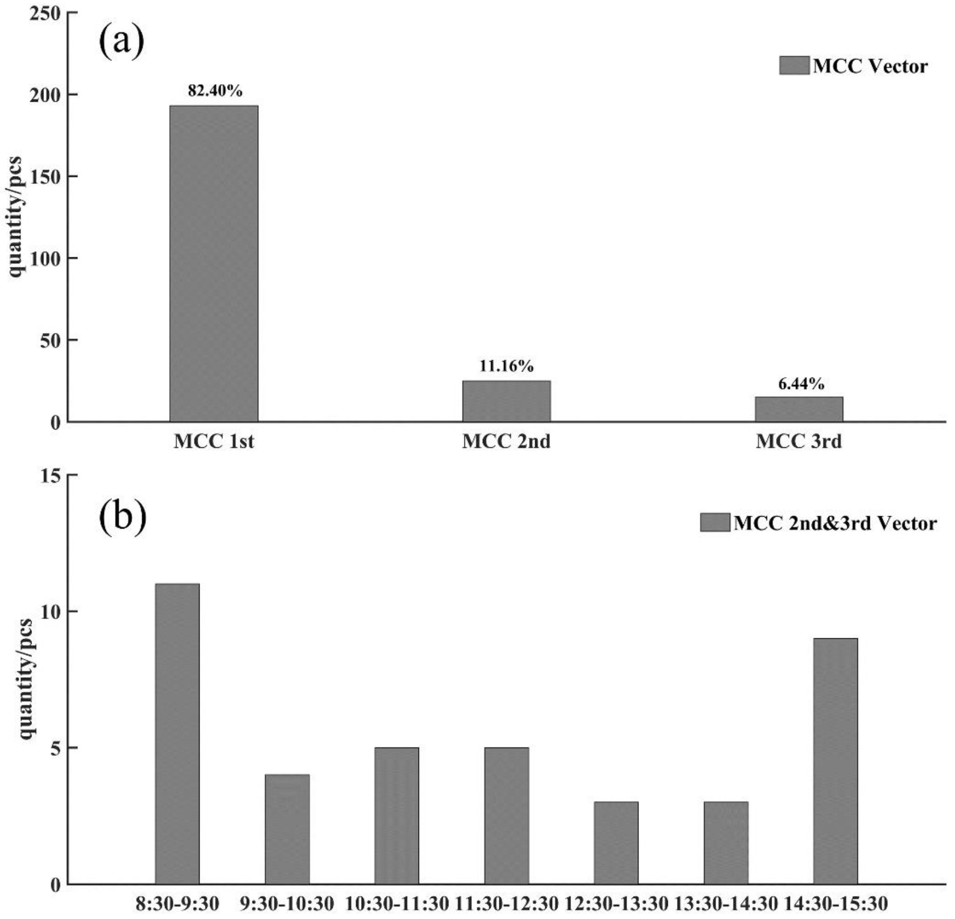
5.1. The Proportion of Accurate Vectors
5.2. Window Size Selection
5.3. Condition Analysis of Current Detection
6. Conclusions
Author Contributions
Funding
Data Availability Statement
Conflicts of Interest
References
- Paduan, J.D.; Washburn, L. High-frequency radar observations of ocean surface currents. Annu. Rev. Mar. Sci. 2013, 5, 115–136. [Google Scholar] [CrossRef]
- Klemas, V. Remote Sensing of Coastal and Ocean Currents: An Overview. J. Coast. Res. 2012, 28, 576–586. [Google Scholar] [CrossRef]
- Jin, Y. Remote Sensing Analysis of Sea Surface Current of Radial Sand Ridges Based on GOCI. Geospat. Inf. 2017, 15, 37–40. [Google Scholar] [CrossRef]
- Lou, X.; Shi, A.; Zhang, H. Coastal sea surface current observation with GOCI imagery. In Proceedings of the Eighth International Symposium on Multispectral Image Processing and Pattern Recognition, Wuhan, China, 10 October 2013. [Google Scholar] [CrossRef]
- Hu, Z.; Pan, D.; He, X.; Bai, Y. Diurnal Variability of Turbidity Fronts Observed by Geostationary Satellite Ocean Color Remote Sensing. Remote Sens. 2016, 8, 147. [Google Scholar] [CrossRef]
- Sun, H.; Zhou, H.; Zhang, Z.; Zhang, Y.; Wang, H. Research on the estimation method of near real-time global ocean surface flow field. J. Mar. Technol. 2015, 34, 1–5. [Google Scholar]
- Amin, R.; Lewis, M.; Lawson, A.; Gould, R.; Martinolich, P.; Li, R.R.; Ladner, S.; Gallegos, S. Comparative Analysis of GOCI Ocean Color Products. Sensors 2015, 15, 25703–25715. [Google Scholar] [CrossRef]
- Yang, H.; Arnone, R.; Jolliff, J. Estimating advective near-surface currents from ocean color satellite images. Remote Sens. Environ. 2015, 158, 1–14. [Google Scholar] [CrossRef]
- Choi, J.K.; Yang, H.; Han, H.J.; Ryu, J.H.; Park, Y.J. Quantitative estimation of suspended sediment movements in coastal region using GOCI. J. Coast. Res. 2016, SI, 1367–1372. [Google Scholar] [CrossRef]
- Yang, H.; Choi, J.K.; Park, Y.J.; Han, H.J.; Ryu, J.H. Application of the Geostationary Ocean Color Imager (GOCI) to estimates of ocean surface currents. J. Geophys. Res. Ocean. 2014, 119, 3988–4000. [Google Scholar] [CrossRef]
- Castellanos, P.; Pelegri, J.L.; Baldwin, D.; Emery, W.J.; Hernandez-Guerra, A. Winter and spring surface velocity fields in the Cape Blanc region as deduced with the maximum cross-correlation technique. Int. J. Remote Sens. 2013, 34, 3587–3606. [Google Scholar] [CrossRef]
- Marcello, J.; Eugenio, F.; Marques, F.; Hernandez-Guerra, A.; Gasull, A. Motion Estimation Techniques to Automatically Track Oceanographic Thermal Structures in Multisensor Image Sequences. IEEE Trans. Geosci. Remote Sens. 2008, 46, 2743–2762. [Google Scholar] [CrossRef]
- Tokmakian, R.; Strub, P.T.; Mcclean-Padman, J. Evaluation of the Maximum Cross-Correlation Method of Estimating Sea Surface Velocities from Sequential Satellite Images. J. Atmos. Ocean. Technol. 1990, 7, 852–865. [Google Scholar] [CrossRef]
- Chen, W.; Mied, R.P.; Gao, B.C.; Wagner, E. Surface Velocities From Multiple-Tracer Image Sequences. IEEE Geosci. Remote Sens. Lett. 2012, 9, 769–773. [Google Scholar] [CrossRef]
- Kelly; Kathryn, A. An Inverse Model for Near-Surface Velocity from Infrared Images. J. Phys. Oceanogr. 1989, 19, 1845–1864. [Google Scholar] [CrossRef]
- Chen, W. Nonlinear inverse model for velocity estimation from an image sequence. J. Geophys. Res. Ocean. 2011, 116, C6. [Google Scholar] [CrossRef]
- Barton; Ian, J. Ocean Currents from Successive Satellite Images: The Reciprocal Filtering Technique. J. Atmos. Ocean. Technol. 2002, 19, 1677–1689. [Google Scholar] [CrossRef]
- Emery, W.J.; Thomas, A.C.; Collins, M.J.; Crawford, W.R.; Mackas, D.L. An objective method for computing advective surface velocities from sequential infrared satellite images. J. Geophys. Res. Ocean. 1986, 91, 12865–12878. [Google Scholar] [CrossRef]
- Kelly, K.A.; Strub, P.T. Comparison of velocity estimates from advanced very high resolution radiometer in the Coastal Transition Zone. J. Geophys. Res. Ocean. 1992, 97, 9653–9668. [Google Scholar] [CrossRef]
- Notarstefano, G.; Poulain, P.M.; Mauri, E. Estimation of Surface Currents in the Adriatic Sea from Sequential Infrared Satellite Images. J. Atmos. Ocean. Technol. 2008, 25, 271–285. [Google Scholar] [CrossRef]
- Gao, J.; Lythe, M.B. The Maximum Cross-Correlation approach to detecting translational motions from sequential remote-sensing images. Comput. Geosci. 1996, 22, 525–534. [Google Scholar] [CrossRef]
- Garcia, C.; Robinson, I.S. Sea Surface Velocities in Shallow Seas Extracted From Sequential Coastal Zone Color Scanner Satellite Data. J. Geophys. Res. Ocean. 1989, 94, 12681–12691. [Google Scholar] [CrossRef]
- Zhu, Z.; Geng, X.; Li, S.; Xie, T.; Yan, X.-H. Ocean surface current retrieval at Hangzhou Bay from Himawari-8 sequential satellite images. Sci. China (Earth Sci.) 2020, 63, 132–144. [Google Scholar] [CrossRef]
- Sun, H.; Song, Q.; Shao, R.; Schlicke, T. Estimation of sea surface currents based on ocean colour remote-sensing image analysis. Int. J. Remote Sens. 2016, 37, 5105–5121. [Google Scholar] [CrossRef]
- Lang, W.; Wu, Q.; Zhang, X.; Meng, J.; Wang, N.; Cao, Y. Sea ice drift tracking in the Bohai Sea using geostationary ocean color imagery. J. Appl. Remote Sens. 2014, 8, 83650. [Google Scholar] [CrossRef]
- Chen, J.; Chen, J.; Cao, Z.; Shen, Y. Improving Surface Current Estimation From Geostationary Ocean Color Imager Using Tidal Ellipse and Angular Limitation. J. Geophys. Res. Ocean. 2019, 124, 4322–4333. [Google Scholar] [CrossRef]
- Jiang, L.; Wang, M. Diurnal Currents in the Bohai Sea Derived From the Korean Geostationary Ocean Color Imager. IEEE Trans. Geosci. Remote Sens. 2017, 55, 1437–1450. [Google Scholar] [CrossRef]
- Wang, D. An Objective Method with a Continuity Constraint for Improving Surface Velocity Estimates from the Geostationary Ocean Color Imager. Remote Sens. 2021, 14, 14. [Google Scholar] [CrossRef]
- Hu, Z.; Pan, D.; He, X.; Song, D.; Huang, N.; Bai, Y.; Xu, Y.; Wang, X.; Zhang, L.; Gong, F. Assessment of the MCC method to estimate sea surface currents in highly turbid coastal waters from GOCI. Int. J. Remote Sens. 2016, 38, 572–597. [Google Scholar] [CrossRef]
- Egbert, G.D.; Bennett, A.F.; Foreman, M. TOPEX/POSEIDON tides estimated using a global inverse model. J. Geophys. Res. Atmos. 1994, 99, 821–852. [Google Scholar] [CrossRef]
- Egbert, G.D.; Erofeeva, S.Y. Efficient Inverse Modeling of Barotropic Ocean Tides. J. Atmos. Ocean. Technol. 2002, 19, 183–204. (accessed on 20 June 2022). [Google Scholar] [CrossRef]
- Hu, Z.; Wang, D.P.; Pan, D.; He, X.; Miyazawa, Y.; Bai, Y.; Wang, D.; Gong, F. Mapping surface tidal currents and Changjiang plume in the East China Sea from G eostationary Ocean Color I mager. J. Geophys. Res. Ocean. 2016, 121, 1563–1572. [Google Scholar] [CrossRef]
- Zhao, Q.; Hou, G.; Tang, Z.; Shu, Z. Accuracy assessment of seven numerical models on simulating tides in the coastal area of Zhejiang. Adv. Mar. Sci. 2018, 36, 310–320. [Google Scholar]
- Cui, H.; Chen, J.; Cao, Z.; Guan, W.; Zhu, Q.; Gong, F. Study on applicability of GOCI inversion and OSU model sea surface currents field data in the Yellow Sea tidal wave system. Haiyang Xuebao 2022, 44, 93–108. [Google Scholar] [CrossRef]
- Davis; Russ, E. Drifter observations of coastal surface currents during CODE: The method and descriptive view. J. Geophys. Res. Atmos. 1985, 90, 4741–4755. [Google Scholar] [CrossRef]
- Choi, J.K.; Park, Y.J.; Ahn, J.H.; Lim, H.S.; Eom, J.; Ryu, J.H. GOCI, the world’s first geostationary ocean color observation satellite, for the monitoring of temporal variability in coastal water turbidity. J. Geophys. Res. Ocean. 2012, 117, C9. [Google Scholar] [CrossRef]
- Padman, L.; Erofeeva, S. Tide Model Driver (TMD) Manual. Earth and Space Research 2005. Available online: www.esr.org/polar_tide_models/README_TMD.pdf (accessed on 14 July 2021).
- Ryu, J.H.; Han, H.J.; Cho, S.; Park, Y.J.; Ahn, Y.H. Overview of geostationary ocean color imager (GOCI) and GOCI data processing system (GDPS). Ocean Sci. J. 2012, 47, 223–233. [Google Scholar] [CrossRef]
- Satish, B.; Jayakrishnan, P. Hardware implementation of template matching algorithm and its performance evaluation. In Proceedings of the 2017 International Conference on Microelectronic Devices, Circuits and Systems (ICMDCS), Vellore, India, 10–12 August 2017. [Google Scholar] [CrossRef]
- Chen, W. Surface Velocity Estimation From Satellite Imagery Using Displaced Frame Central Difference Equation. IEEE Trans. Geosci. Remote Sens. 2012, 50, 2791–2801. [Google Scholar] [CrossRef]
- Lie, H.-J.; Lee, S.; Cho, C.-H. Computation methods of major tidal currents from satellite-tracked drifter positions, with application to the Yellow and East China Seas. J. Geophys. Res. Ocean. 2002, 107, 3-1-3-22. [Google Scholar] [CrossRef]
- Zhu, X.; Liu, G. Numerical study on the tides and tidal currents in Bohai Sea, Yellow Sea and East China Sea. Oceanol. Et Limnol. Sin. 2012, 43, 1103–1113. [Google Scholar] [CrossRef]
- Chao, M.; Wu, D.; Lin, X. Variability of surface velocity in the Kuroshio Current and adjacent waters derived from Argos drifter buoys and satellite altimeter data. Chin. J. Oceanol. Limnol. 2009, 27, 208–217. [Google Scholar] [CrossRef]
- Zhu, X.; Liu, G. Numerical study on the tidal currents, tidal energy fluxes and dissipation in the China Seas. Oceanol. Et Limnol. Sin. 2012, 43, 669–677. [Google Scholar] [CrossRef]
- Su, M.; Yao, P.; Wang, Z.B.; Zhang, C.K.; Stive, M.J. Tidal wave propagation in the Yellow Sea. Coast. Eng. J. 2015, 57, 1550008. [Google Scholar] [CrossRef]
- Shen, Y.; Huang, D.; Qian, C. A tentative interpretation of the formation mechanism of the semidiurnal tidal wave system in the Yellow Sea. Haiyang Xuebao 1993, 15, 16–24. [Google Scholar]
- Li, H.; He, X.; Tao, B.; Wang, D. Research on chlorophyll detection ability under high solar zenith angle. Haiyang Xuebao 2018, 40, 128–140. [Google Scholar] [CrossRef]
- Crocker, R.I.; Matthews, D.K.; Emery, W.J.; Baldwin, D.G. Computing Coastal Ocean Surface Currents From Infrared and Ocean Color Satellite Imagery. IEEE Trans. Geosci. Remote Sens. 2007, 45, 435–447. [Google Scholar] [CrossRef]


| Area | Time | Original Data | Angular Limitation Filter | Multi-Correlation Coefficient Optimization | |||
|---|---|---|---|---|---|---|---|
| AME | AAE (°) | AME | AAE (°) | AME | AAE (°) | ||
| ECS | 10 August | 0.27 | 18.83 | 0.26 | 13.35 | 0.23 | 13.43 |
| 11 August | 0.34 | 55.01 | 0.25 | 49.42 | 0.26 | 49.84 | |
| 13 August | 0.78 | 33.16 | 0.86 | 19.42 | 0.75 | 18.92 | |
| SYS | 27 June | 0.34 | 40.46 | 0.37 | 40.08 | 0.33 | 38.14 |
| 11 July | 0.61 | 34.89 | 0.62 | 26.93 | 0.61 | 25.84 | |
| 16 July | 1.61 | 42.87 | 1.50 | 46.99 | 1.45 | 30.39 | |
| NYS | 5 August | 0.40 | 16.66 | 0.40 | 11.26 | 0.41 | 14.08 |
| 6 August | 0.47 | 66.88 | 0.47 | 72.31 | 0.52 | 54.83 | |
| 7 August | 0.35 | 31.59 | 0.40 | 31.25 | 0.38 | 27.06 | |
| Average | 0.57 | 37.82 | 0.57 | 34.56 | 0.55 | 30.28 | |
| Buoy Number | Number of Sites | BUOY-ACS (m/s) | OSU-ACS (m/s) | AAE (°) |
|---|---|---|---|---|
| 1132711 | 1759 | 0.43 | 0.41 | 44.16 |
| 1131901 | 1787 | 0.28 | 0.34 | 49.90 |
| 1227890 | 320 | 0.45 | 0.38 | 37.82 |
| Average | 1289 | 0.39 | 0.38 | 43.96 |
| MCC | W (=H) | W1 | W2 | W3 | W4 | W5 | W6 | W7 |
|---|---|---|---|---|---|---|---|---|
| Tsub | pixels | 10 | 10 | 20 | 20 | 28 | 20 | 28 |
| Ssub | pixels | 24 | 36 | 24 | 36 | 36 | 48 | 48 |
| W1 | W2 | W3 | W4 | W5 | W6 | W7 | |
|---|---|---|---|---|---|---|---|
| Max-speed (m/s) | 1.11 | 2.95 | 1.57 | 1.39 | 1.18 | 2.95 | 1.46 |
| Min-speed (m/s) | 0.23 | 0.36 | 0.79 | 0.22 | 0.01 | 0.15 | 0.05 |
| Ave-speed (m/s) | 0.60 | 1.09 | 1.00 | 0.68 | 0.28 | 0.74 | 0.51 |
| PCV (%) | 86.54 | 97.65 | 56.20 | 96.58 | 70.09 | 87.61 | 77.56 |
| Target Vector | W1 | W2 | W3 | W4 | ||||
|---|---|---|---|---|---|---|---|---|
| AME | AAE(°) | AME | AAE(°) | AME | AAE(°) | AME | AAE(°) | |
| Ⅰ | 0.07 | 10.43 | 0.10 | 9.70 | 0.09 | 2.08 | 0.09 | 13.63 |
| Ⅱ | 0.24 | 54.72 | 0.36 | 42.48 | —— | —— | 0.76 | 39.24 |
| Ⅲ | 0.07 | 16.70 | 0.26 | 29.73 | —— | —— | 0.45 | 29.94 |
| Average | 0.13 | 27.28 | 0.24 | 27.31 | —— | —— | 0.43 | 27.60 |
| Target Vector | W5 | W6 | W7 | |||||
| AME | AAE(°) | AME | AAE(°) | AME | AAE(°) | |||
| Ⅰ | 0.20 | 5.21 | 0.10 | 13.18 | 0.13 | 11.76 | ||
| Ⅱ | 6.61 | 59.76 | 0.69 | 56.20 | 0.38 | 20.41 | ||
| Ⅲ | 0.46 | 23.16 | 0.49 | 32.10 | —— | —— | ||
| Average | 2.42 | 29.37 | 0.43 | 33.83 | —— | —— | ||
| Date | Time | Chl-a | Rrs | TSM | ||||||
|---|---|---|---|---|---|---|---|---|---|---|
| Number of Vectors | AME | AAE (°) | Number of Vectors | AME | AAE (°) | Number of Vectors | AME | AAE (°) | ||
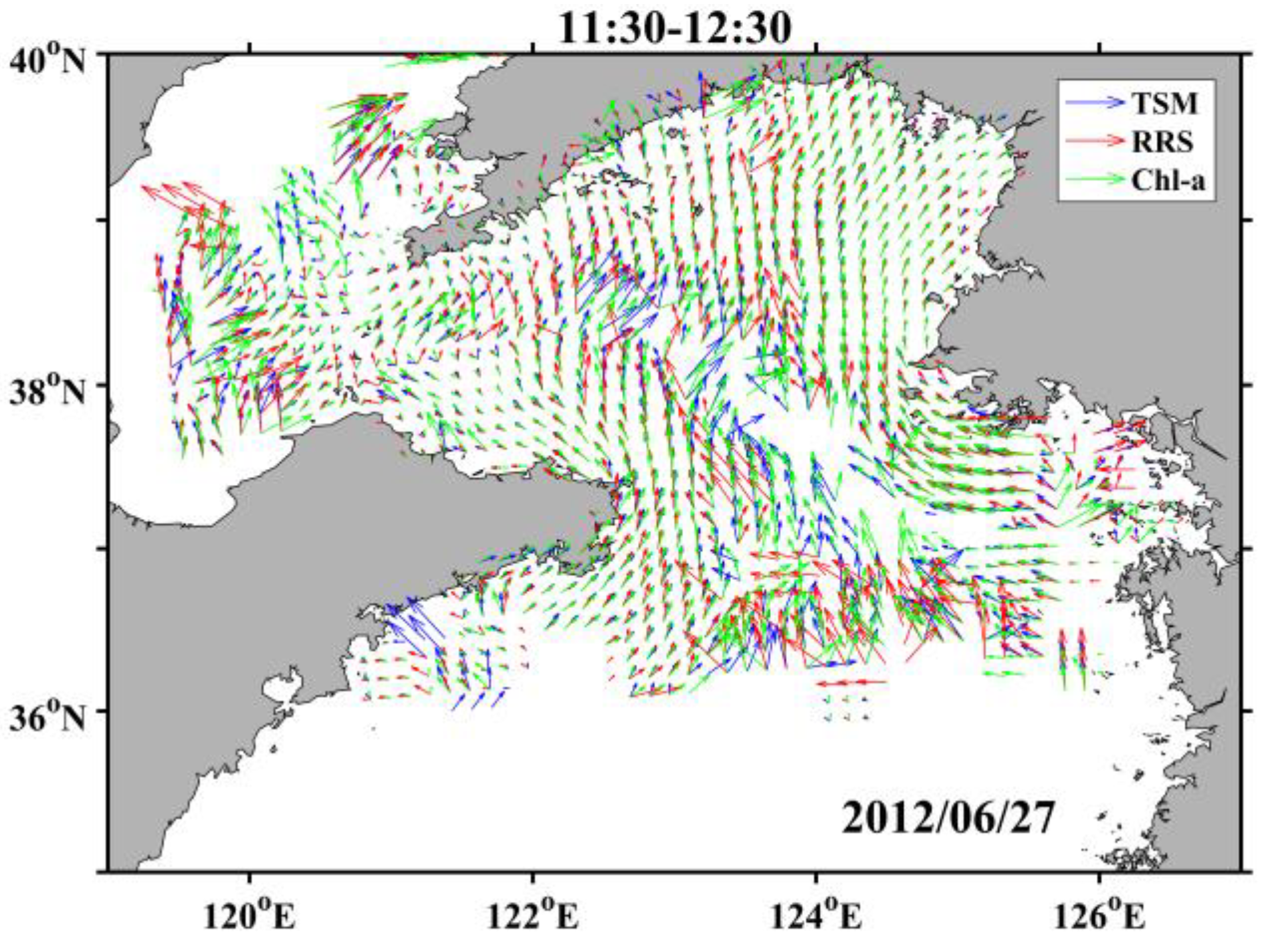
| 27 June | 11:30–12:30 | 1010 | 1.13 | 21.83 | 955 | 1.22 | 27.04 | 1005 | 0.67 | 13.62 |
| 12:30–13:30 | 976 | 1.90 | 27.15 | 952 | 0.54 | 16.17 | 981 | 1.59 | 18.31 | |
| 11 July | 11:30–12:30 | 472 | 0.30 | 13.99 | 448 | 0.62 | 13.51 | 476 | 0.53 | 15.34 |
| 12:30–13:30 | 580 | 0.25 | 6.44 | 487 | 0.50 | 16.10 | 553 | 0.52 | 12.54 | |
| 16 July | 11:30–12:30 | 467 | 0.32 | 24.74 | 464 | 0.76 | 39.16 | 484 | 0.32 | 29.59 |
| 12:30–13:30 | 534 | 0.73 | 15.95 | 503 | 1.42 | 24.14 | 541 | 0.99 | 12.34 | |
| Average | 673 | 0.77 | 18.35 | 634 | 0.84 | 22.69 | 673 | 0.77 | 16.96 | |
Publisher’s Note: MDPI stays neutral with regard to jurisdictional claims in published maps and institutional affiliations. |
© 2022 by the authors. Licensee MDPI, Basel, Switzerland. This article is an open access article distributed under the terms and conditions of the Creative Commons Attribution (CC BY) license (https://creativecommons.org/licenses/by/4.0/).
Share and Cite
Cui, H.; Chen, J.; Cao, Z.; Huang, H.; Gong, F. A Novel Multi-Candidate Multi-Correlation Coefficient Algorithm for GOCI-Derived Sea-Surface Current Vector with OSU Tidal Model. Remote Sens. 2022, 14, 4625. https://doi.org/10.3390/rs14184625
Cui H, Chen J, Cao Z, Huang H, Gong F. A Novel Multi-Candidate Multi-Correlation Coefficient Algorithm for GOCI-Derived Sea-Surface Current Vector with OSU Tidal Model. Remote Sensing. 2022; 14(18):4625. https://doi.org/10.3390/rs14184625
Chicago/Turabian StyleCui, He, Jianyu Chen, Zhenyi Cao, Haiqing Huang, and Fang Gong. 2022. "A Novel Multi-Candidate Multi-Correlation Coefficient Algorithm for GOCI-Derived Sea-Surface Current Vector with OSU Tidal Model" Remote Sensing 14, no. 18: 4625. https://doi.org/10.3390/rs14184625