
Characterizing Residual Current Circulation and Its Response Mechanism to Wind at a Seasonal Scale Based on High-Frequency Radar Data
 and
and
Abstract
:1. Introduction
2. Methodologies
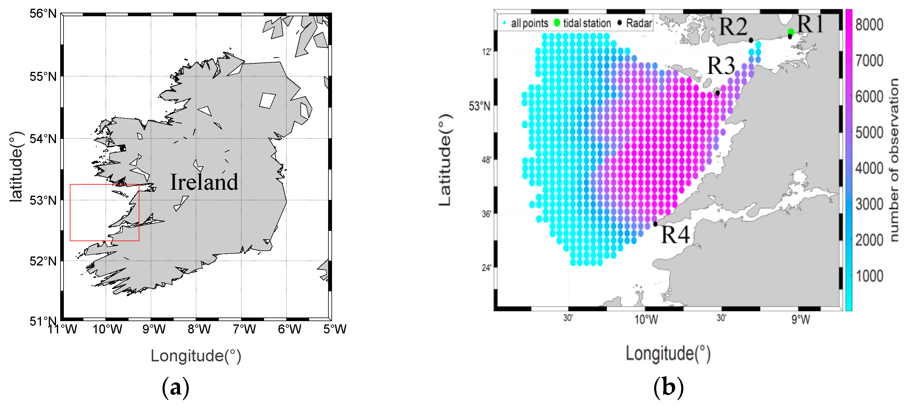
2.1. Study Area
2.2. HFR System
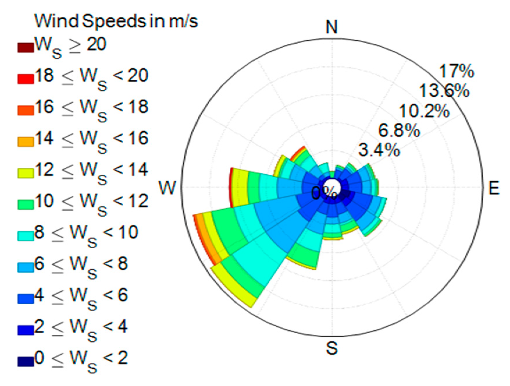
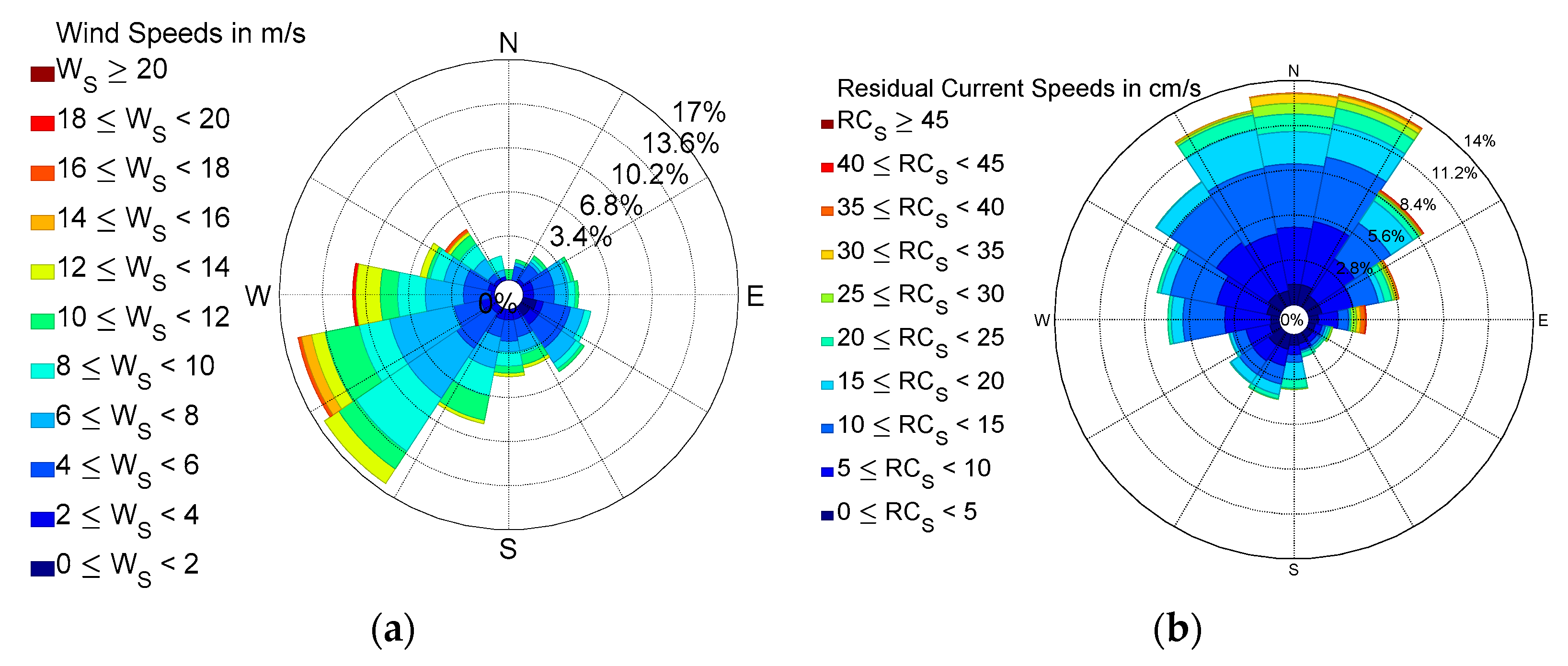
2.3. Atmospheric Data
2.4. Extraction of Residual Surface Currents
3. Results
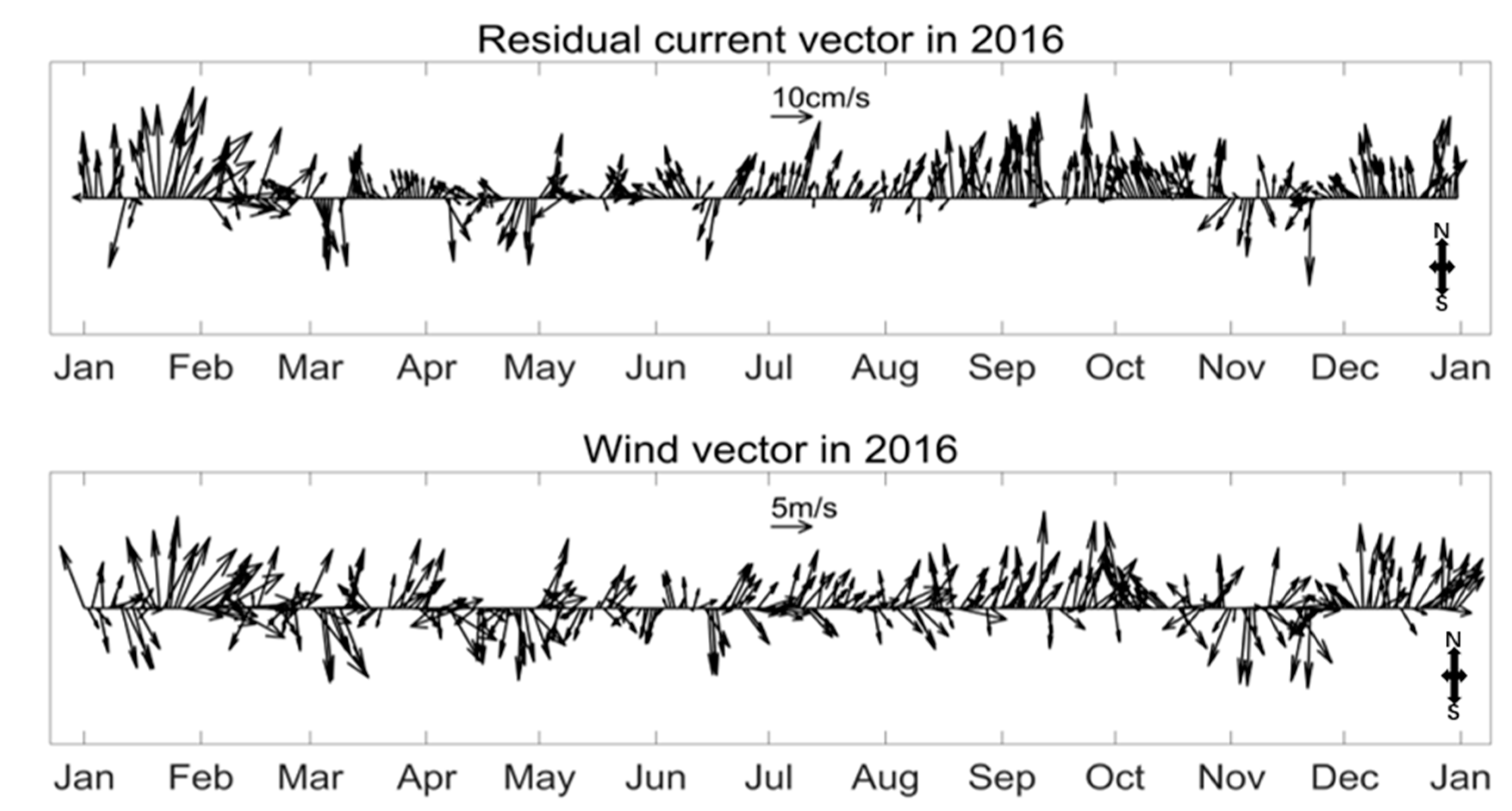
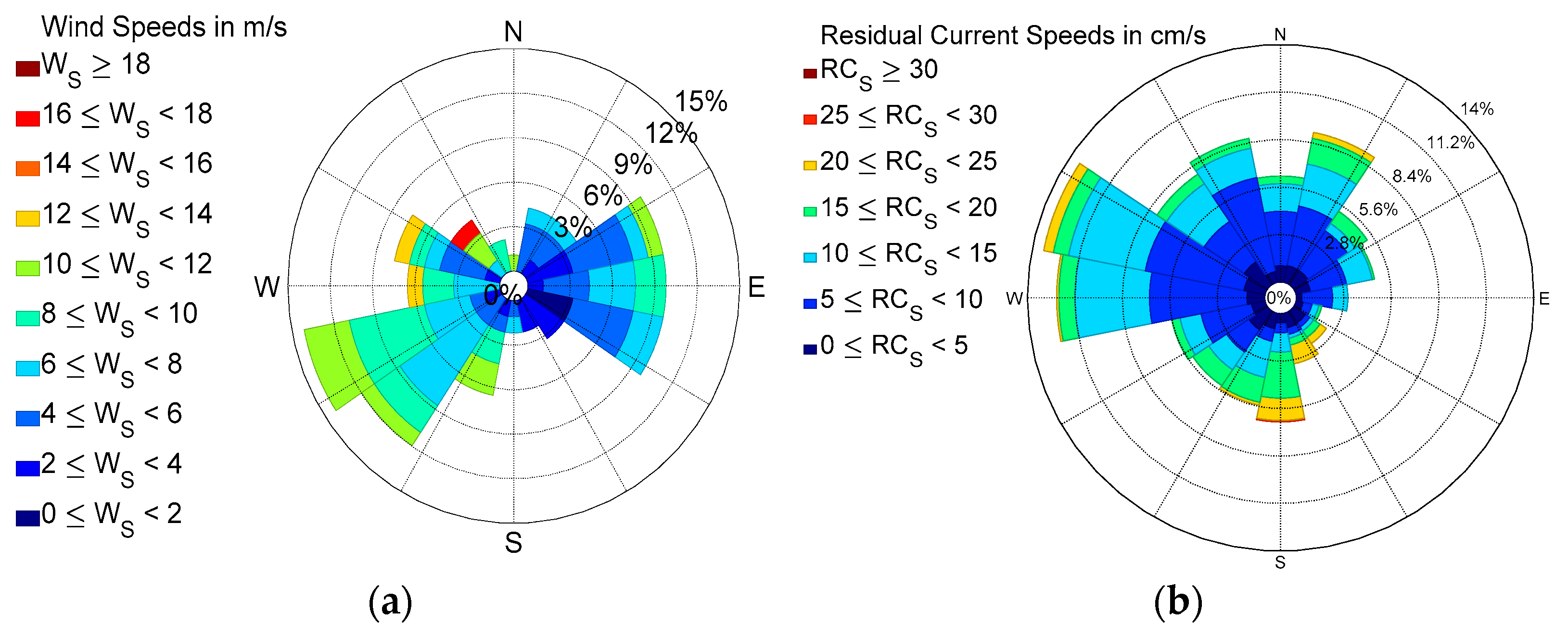
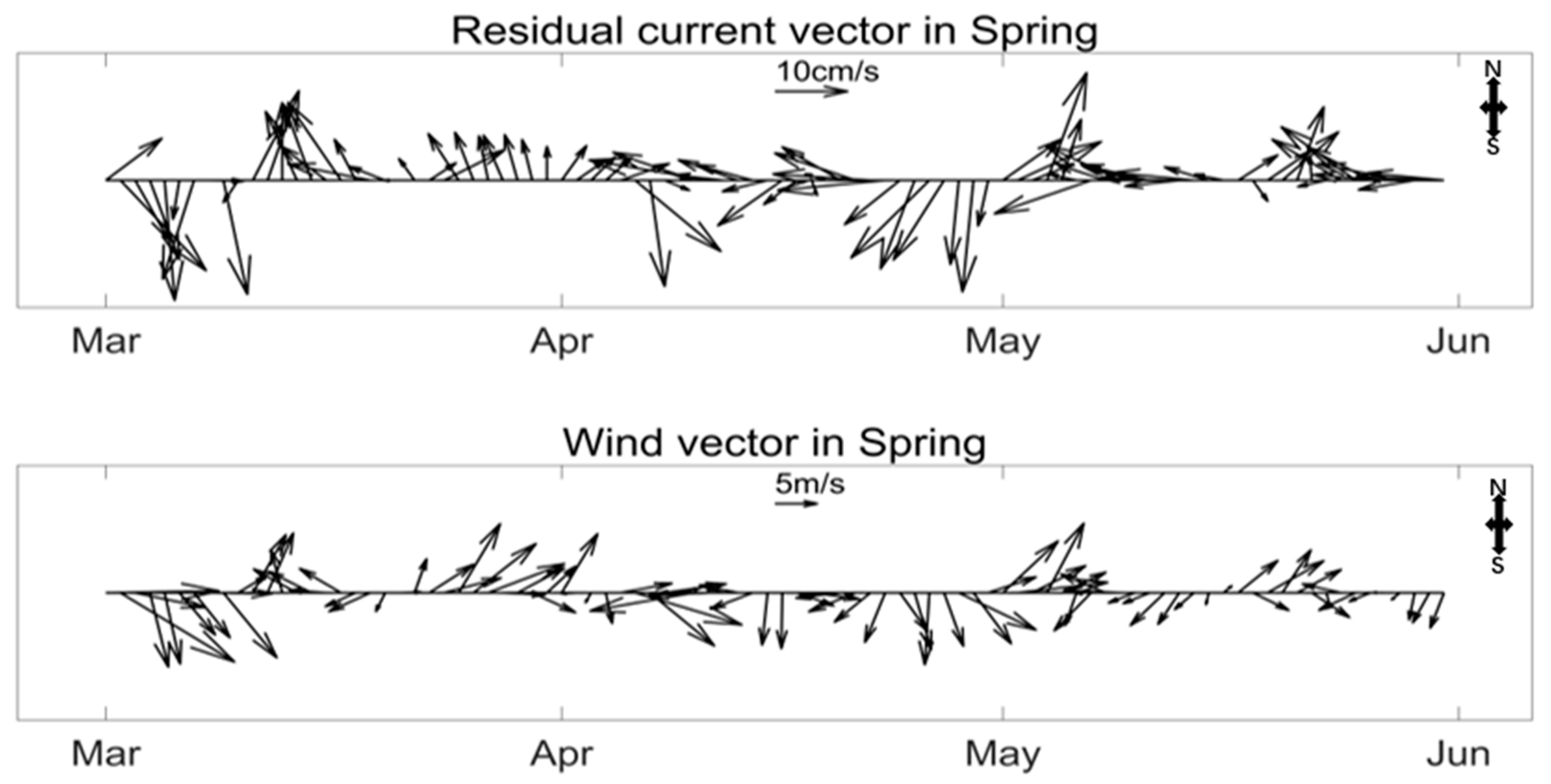
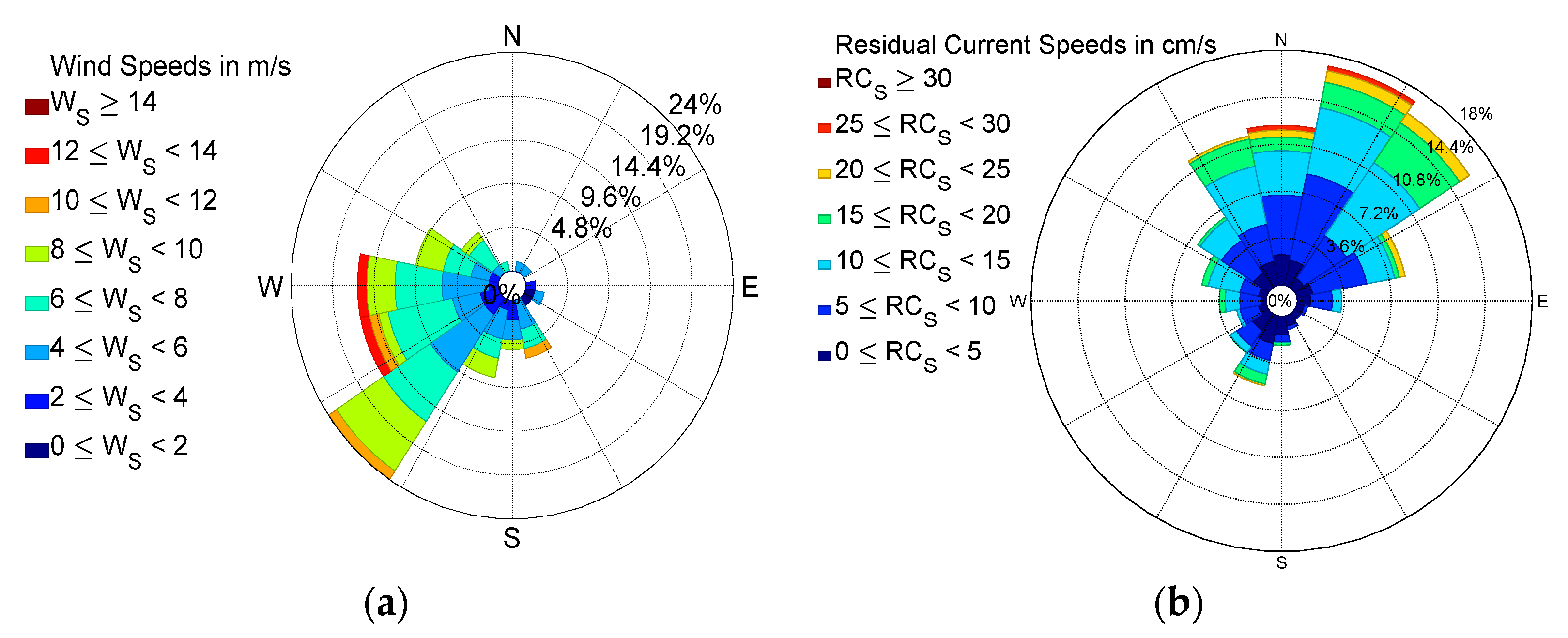
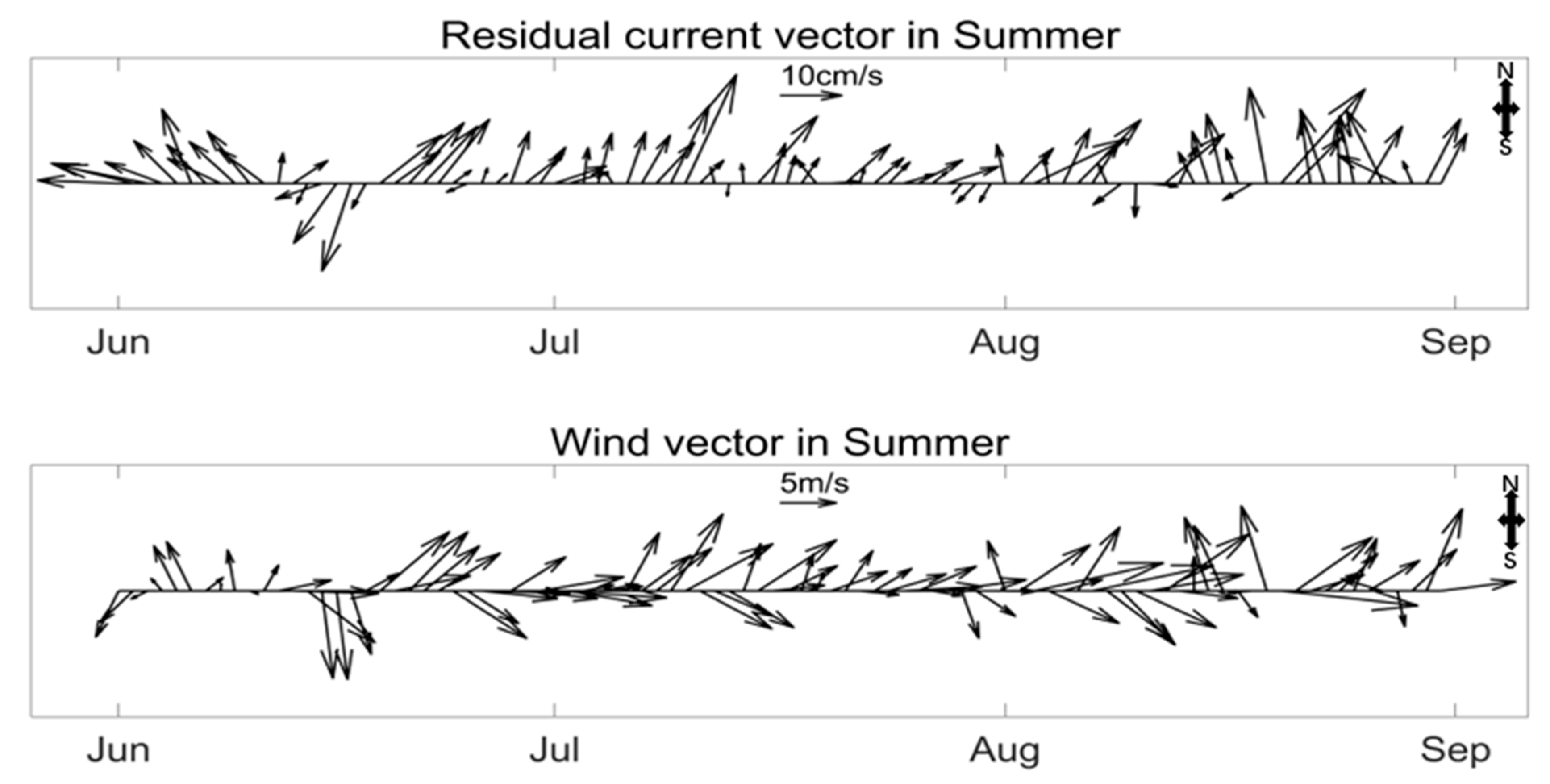
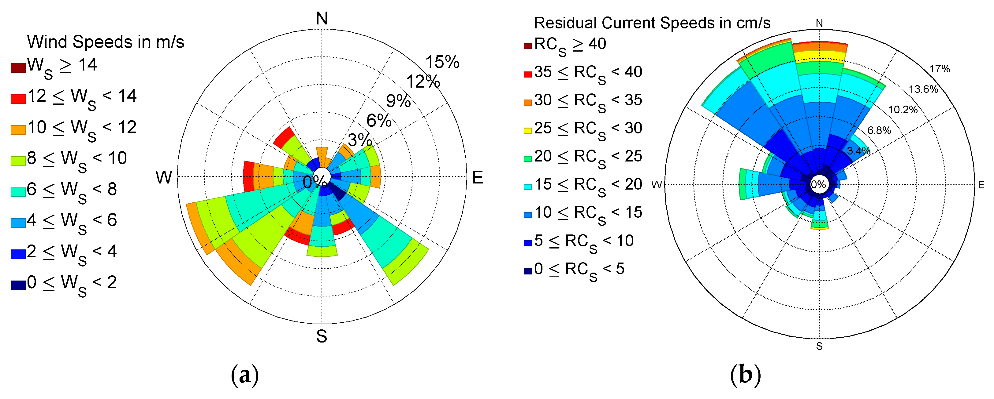
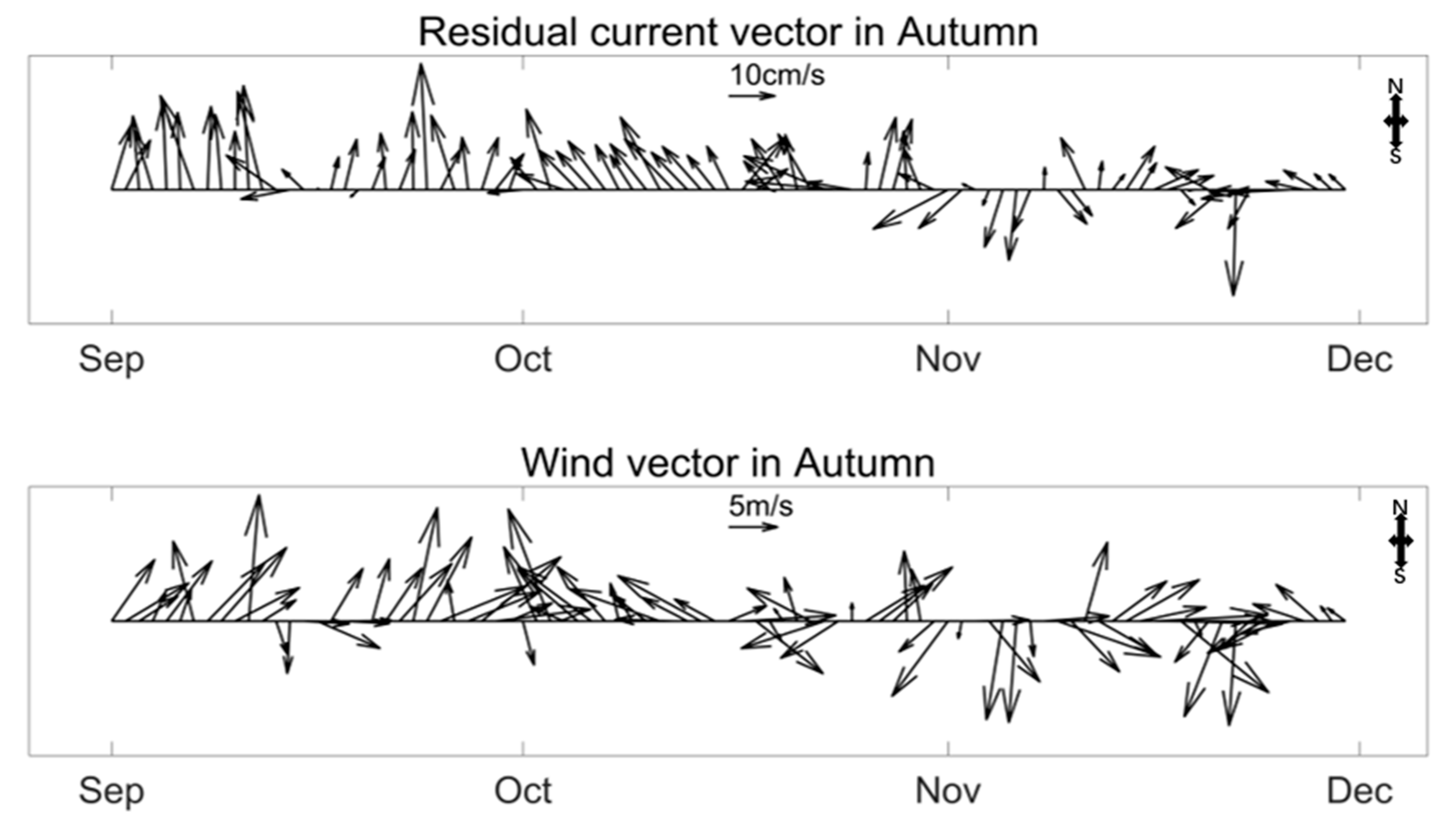
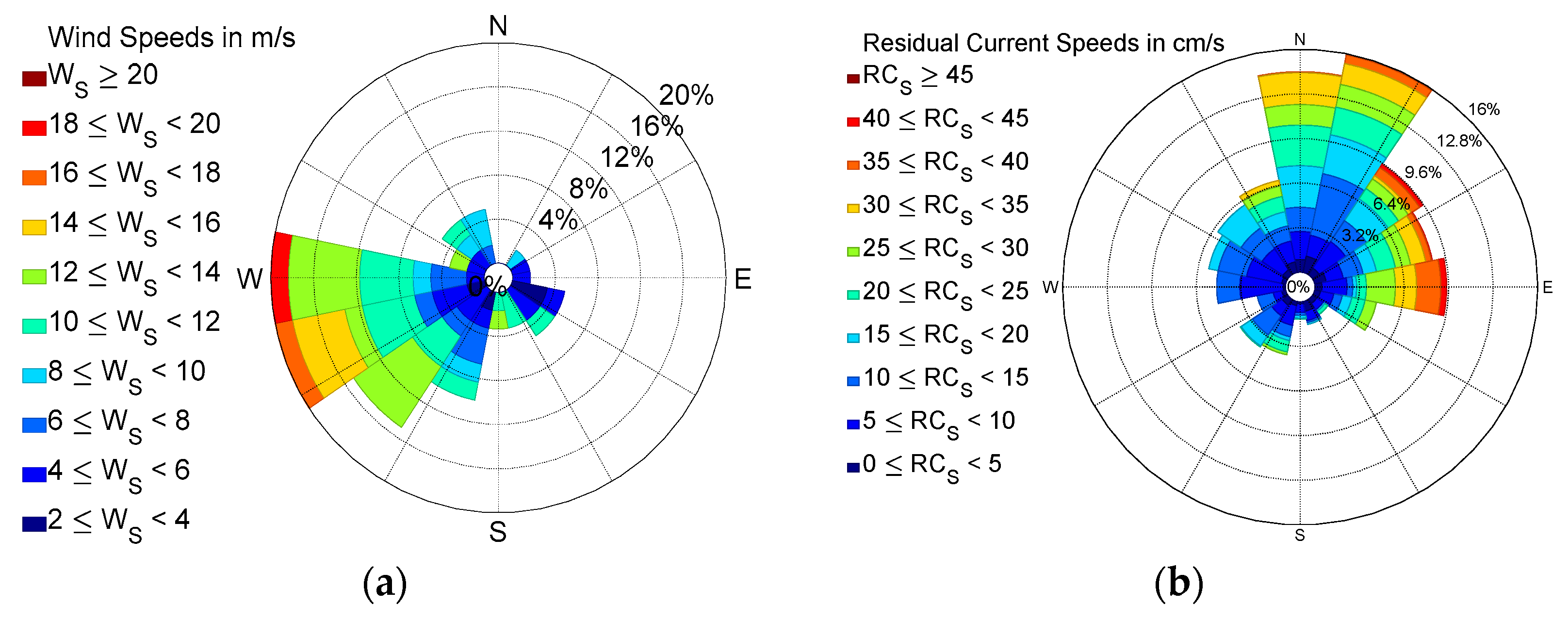
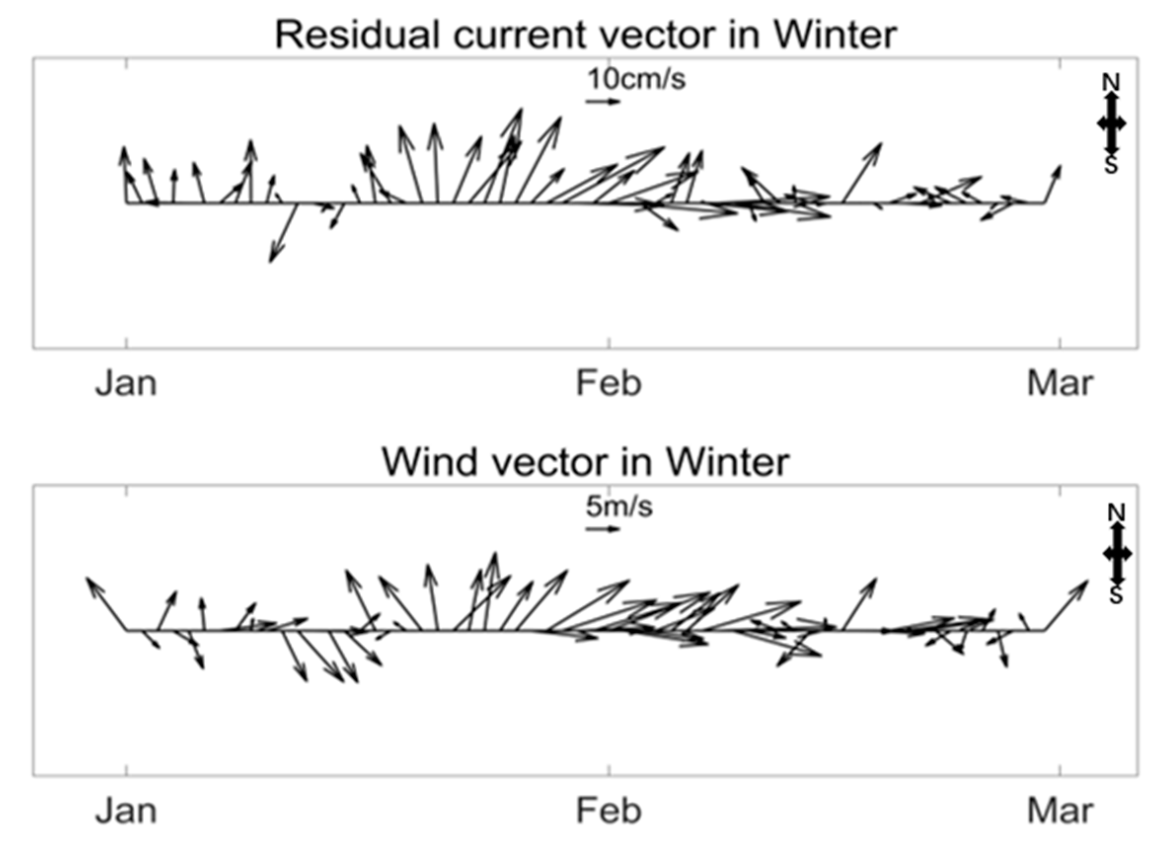
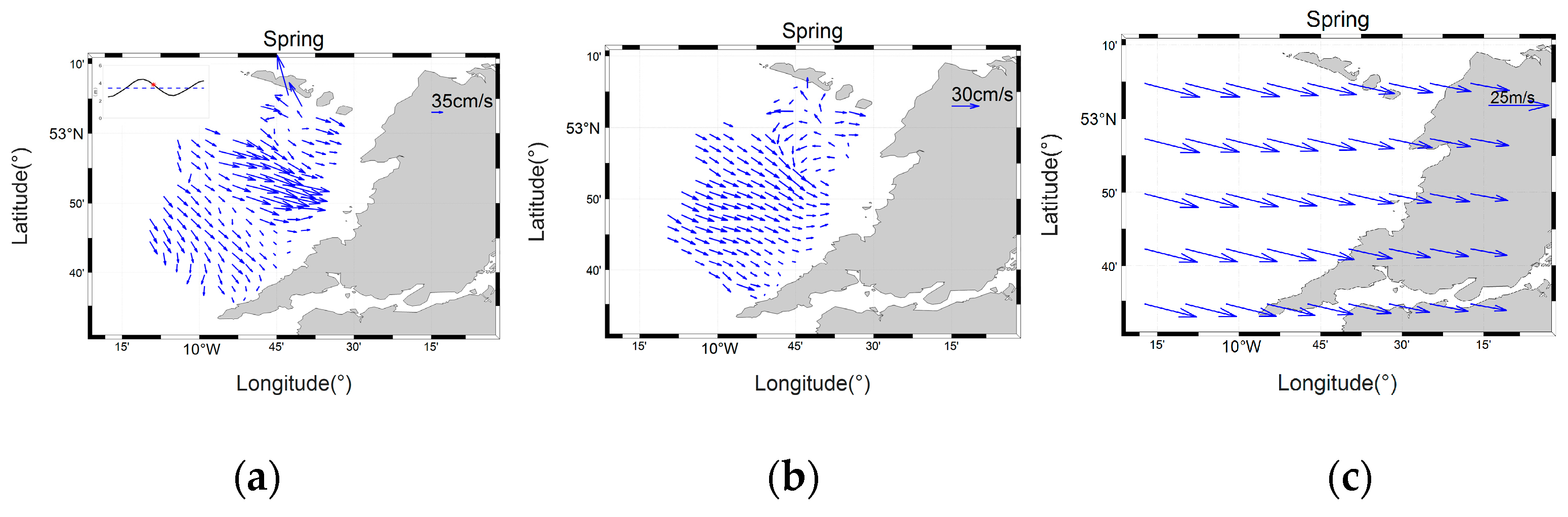
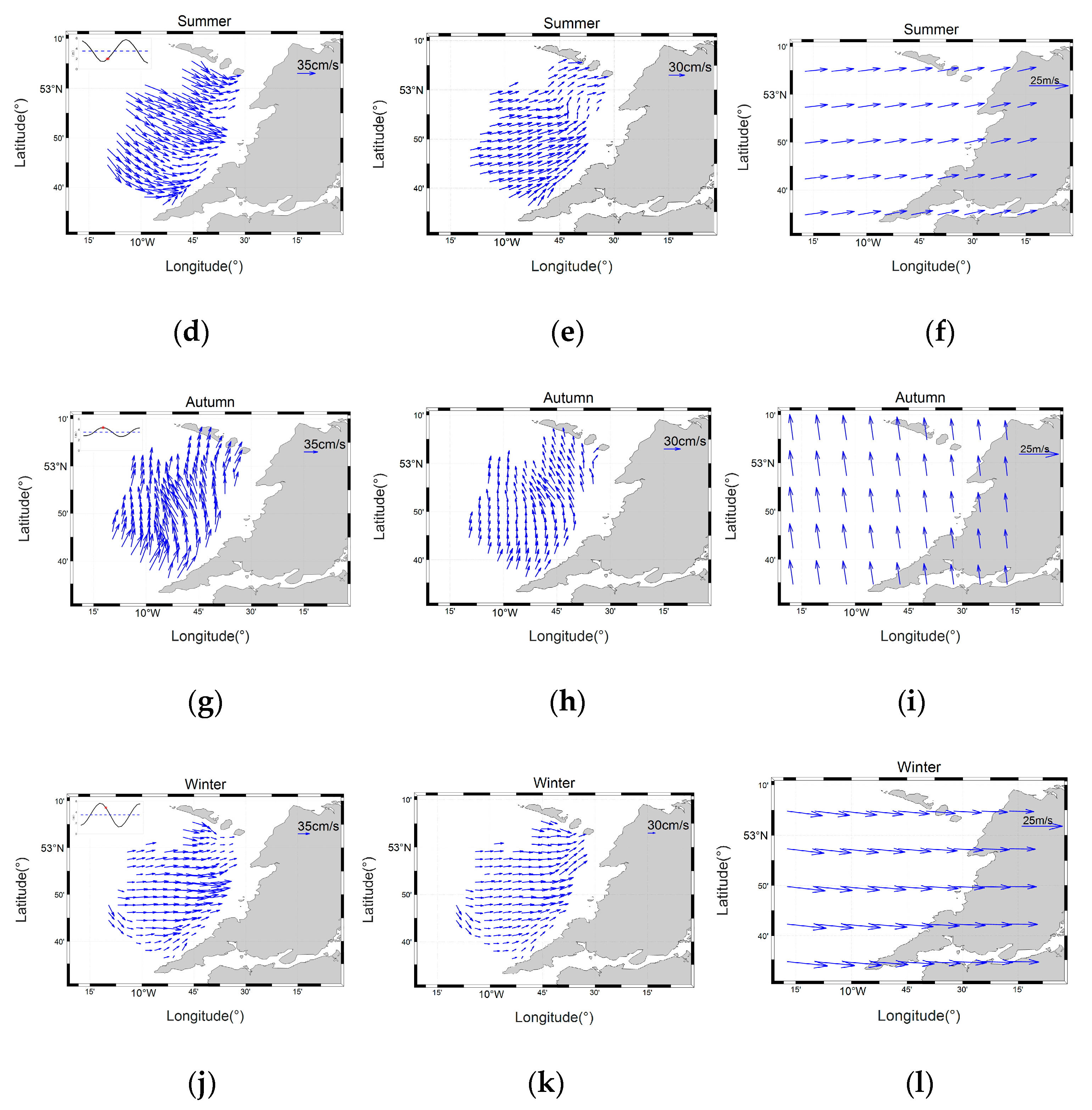
3.1. Response of Residual Surface Currents to Wind
3.2. Influence of the Maximum Wind on Residual Currents
4. Discussion
5. Conclusions
Author Contributions
Funding
Conflicts of Interest
References
- Kim, S.J.; Kõrgersaar, M.; Ahmadi, N.; Taimuri, G.; Kujala, P.; Hirdaris, S. The influence of fluid structure interaction modelling on the dynamic response of ships subject to collision and grounding. Mar. Struct. 2021, 75, 102875. [Google Scholar] [CrossRef]
- Wang, B.; Hirose, N.; Moon, J.-H.; Yuan, D. Difference between the Lagrangian trajectories and Eulerian residual velocity fields in the southwestern Yellow Sea. Ocean Dyn. 2013, 63, 565–576. [Google Scholar] [CrossRef]
- Shi, M.C. Physical Oceanography; Shandong Education Press: Jinan, China, 2005; Volume 60–120. [Google Scholar]
- Yang, J.; Ding, W.; Cui, J.; Guo, S.; Iop. Characteristical analysis of tidal and residual currents in the sea area around Tangshan international tourism island. In Proceedings of the Asia Conference on Geological Research and Environmental Technology (GRET), Electr Network, Kamakura City, Japan, 10–11 October 2020. [Google Scholar] [CrossRef]
- Liu, G.; Liu, Z.; Gao, H.; Gao, Z.; Feng, S. Simulation of the Lagrangian tide-induced residual velocity in a tide-dominated coastal system: A case study of Jiaozhou Bay, China. Ocean Dyn. 2012, 62, 1443–1456. [Google Scholar] [CrossRef]
- Kim, S.Y.; Cornuelle, B.D.; Terrill, E.J. Decomposing observations of high-frequency radar-derived surface currents by their forcing mechanisms: Locally wind-driven surface currents. J. Geophys. Res. Earth Surf. 2010, 115, C12046. [Google Scholar] [CrossRef]
- Holloway, G. Systematic forcing of large-scale geophysical flows by eddy-topography interaction. J. Fluid Mech. 1987, 184, 463–476. [Google Scholar] [CrossRef]
- Callies, U.; Gaslikova, L.; Kapitza, H.; Scharfe, M. German Bight residual current variability on a daily basis: Principal components of multi-decadal barotropic simulations. Geo-Mar. Lett. 2017, 37, 151–162. [Google Scholar] [CrossRef]
- Cheng, P.; Valle-Levinson, A. Influence of Lateral Advection on Residual Currents in Microtidal Estuaries. J. Phys. Oceanogr. 2009, 39, 3177–3190. [Google Scholar] [CrossRef]
- Dong, N.; Wang, G. Residual Current Analysis of the Yellow River Mouth Area in Bohai Gulf. J. Oceanogr. Huanghai Bohai Seas 1997, 15, 64–69. [Google Scholar]
- Matte, P.; Secretan, Y.; Morin, J. Drivers of residual and tidal flow variability in the St. Lawrence fluvial estuary: Influence on tidal wave propagation. Cont. Shelf Res. 2019, 174, 158–173. [Google Scholar] [CrossRef]
- Kilbourne, B.F. On the Topic of Oceanic Variability near the Coriolis Frequency; Generation Mechanisms, Observations, and Implications for Interior Mixing; Research Works Archive, University Libraries, University of Washington: Siettle, WA, USA, 2015; p. 150. [Google Scholar]
- Bradbury, M.C.; Conley, D.C. Using Artificial Neural Networks for the Estimation of Subsurface Tidal Currents from High-Frequency Radar Surface Current Measurements. Remote Sens. 2021, 13, 3896. [Google Scholar] [CrossRef]
- Poul, H.M.; Backhaus, J.; Dehghani, A.; Huebner, U. Effect of subseabed salt domes on Tidal Residual currents in the Persian Gulf. J. Geophys. Res. Ocean. 2016, 121, 3372–3380. [Google Scholar] [CrossRef]
- Dobrynin, M.; Kleine, T.; Düsterhus, A.; Baehr, J. Skilful Seasonal Prediction of Ocean Surface Waves in the Atlantic Ocean. Geophys. Res. Lett. 2019, 46, 1731–1739. [Google Scholar] [CrossRef]
- Gonzalez, P.L.M.; Brayshaw, D.J.; Zappa, G. The contribution of North Atlantic atmospheric circulation shifts to future wind speed projections for wind power over Europe. Clim. Dyn. 2019, 53, 4095–4113. [Google Scholar] [CrossRef]
- Fernand, L.; Nolan, G.D.; Raine, R.; Chambers, C.E.; Dye, S.R.; White, M.; Brown, J. The Irish coastal current: A seasonal jet-like circulation. Cont. Shelf Res. 2006, 26, 1775–1793. [Google Scholar] [CrossRef]
- Han, Q.; Gui, C.; Xu, J.; Lacidogna, G. A generalized method to predict the compressive strength of high-performance concrete by improved random forest algorithm. Constr. Build. Mater. 2019, 226, 734–742. [Google Scholar] [CrossRef]
- Ren, L.; Nagle, D.; Hartnett, M.; Nash, S.J.E. The Effect of Wind Forcing on Modeling Coastal Circulation at a Marine Renewable Test Site. Energies 2017, 10, 2114. [Google Scholar] [CrossRef]
- Gui, R.Z. Adaptively Selecting Working Frequency to Reduce Disturbances in High Frequency Radar. Acta Phys. Pol. A 2011, 119, 473–478. [Google Scholar] [CrossRef]
- Basañez, A.; Pérez-Muñuzuri, V. HF Radars for Wave Energy Resource Assessment Offshore NW Spain. Remote Sens. 2021, 13, 2070. [Google Scholar] [CrossRef]
- Saviano, S.; Esposito, G.; Di Lemma, R.; de Ruggiero, P.; Zambianchi, E.; Pierini, S.; Falco, P.; Buonocore, B.; Cianelli, D.; Uttieri, M. Wind Direction Data from a Coastal HF Radar System in the Gulf of Naples (Central Mediterranean Sea). Remote Sens. 2021, 13, 1333. [Google Scholar] [CrossRef]
- Tseng, Y.-H.; Lu, C.-Y.; Zheng, Q.; Ho, C.-R. Characteristic Analysis of Sea Surface Currents around Taiwan Island from CODAR Observations. Remote Sens. 2021, 13, 3025. [Google Scholar] [CrossRef]
- Cosoli, S.; Mazzoldi, A.; Gačić, M. Validation of Surface Current Measurements in the Northern Adriatic Sea from High-Frequency Radars. J. Atmos. Ocean. Technol. 2010, 27, 908–919. [Google Scholar] [CrossRef]
- Chen, Y.-R.; Paduan, J.D.; Cook, M.S.; Chuang, L.Z.-H.; Chung, Y.-J. Observations of Surface Currents and Tidal Variability Off of Northeastern Taiwan from Shore-Based High Frequency Radar. Remote Sens. 2021, 13, 3438. [Google Scholar] [CrossRef]
- An, Z. Study of Ocean Currents Detection with HF Ground Wave Over-the-Horizon Radar. Ph.D. Thesis, Xidian University, Xi’an, China, 2008. [Google Scholar]
- Xiao, J. Research on Current Data Processing Method of High Frequency Surface Wave Radar. Master’s Thesis, Wuhan University, Wuhan, China, 2017. [Google Scholar]
- Silva, M.T.; Huang, W.; Gill, E.W. Bistatic High-Frequency Radar Cross-Section of the Ocean Surface with Arbitrary Wave Heights. Remote Sens. 2020, 12, 667. [Google Scholar] [CrossRef]
- Novi, L.; Raffa, F.; Serafino, F. Comparison of Measured Surface Currents from High Frequency (HF) and X-Band Radar in a Marine Protected Coastal Area of the Ligurian Sea: Toward an Integrated Monitoring System. Remote Sens. 2020, 12, 3074. [Google Scholar] [CrossRef]
- Lei, R.; Manman, W.; Huayang, C.; Zhan, H.; Qingshu, Y.; Hartnett, M. Characteristics of coastal currents based on High Frequency radar and ADCP observations in the Strait of Georgia. IOP Conf. Ser. Earth Environ. Sci. 2018, 189, 052042. [Google Scholar]
- Shibendu, M.; Rajib, K.; Durbadal, M. Direct digital fractional-order Butterworth filter design using constrained optimization. AEU Int. J. Electron. Commun. 2021, 128, 153511. [Google Scholar]
- Emery, W.J.; Thomson, R.E. Data Analysis Methods in Physical Oceanography, 2nd ed.; Elsevier Science: Amsterdam, The Netherlands, 2001. [Google Scholar]
- Ma, J. Rotary spectrum estimation of ocean current vector time series and its application. ACTA Oceanol. Sin. 1987, 4, 510–518. [Google Scholar]
- Chen, Y. Spatio-Temporal Characteristics and Influencing Factors of Current in Qinhuangdao Coastal Area. Master’s Thesis, Shanghai Ocean University, Shanghai, China, 2019. [Google Scholar]
- Mihanović, H.; Cosoli, S.; Vilibić, I.; Ivanković, D.; Dadić, V.; Gačić, M. Surface current patterns in the northern Adriatic extracted from high-frequency radar data using self-organizing map analysis. J. Geophys. Res. Earth Surf. 2011, 116. [Google Scholar] [CrossRef]
- Wang, H.; Wu, L.; Chai, H.; Xiao, Y.; Hsu, H.; Wang, Y. Characteristics of Marine Gravity Anomaly Reference Maps and Accuracy Analysis of Gravity Matching-Aided Navigation. Sensors 2017, 17, 1851. [Google Scholar] [CrossRef]
- Xing, C.; Zhao, Q.; Cao, X.; Yang, Y.; Song, L. Seasonal variation of the coastal currents in the Northern Bohai Strait. Mar. Environ. Sci. 2020, 39, 334–339. [Google Scholar]
- Hickey, B.M.; Hamilton, P. A Spin-Up Model as a Diagnostic Tool for Interpretation of Current and Density Measurements on the Continental Shelf of the Pacific Northwest. J. Phys. Oceanogr. 1980, 10, 12–24. [Google Scholar] [CrossRef]


| Variable | Statistics | Spring (March–May) | Summer (June–August) | Autumn (September–November) | Winter (December–February) | Full Year |
|---|---|---|---|---|---|---|
| Wind Speed (m/s) | Maximum | 21.31 | 14.28 | 18.26 | 21.96 | 21.96 |
| Average | 6.64 | 6.38 | 7.21 | 9.03 | 7.28 | |
| Minimum | 0.14 | 0.13 | 0.03 | 0.42 | 0.03 | |
| Residual Current Speed (cm/s) | Maximum | 25.12 | 27.17 | 35.65 | 41.18 | 41.18 |
| Average | 10.12 | 9.86 | 12.36 | 16.28 | 11.8 | |
| Minimum | 0.63 | 0.2 | 0.25 | 0.31 | 0.16 |
| Variable | Statistics | Spring | Summer | Autumn | Winter |
|---|---|---|---|---|---|
| Wind Speed (m/s) | Maximum | 25.68 | 16.05 | 21.19 | 27.1 |
| Minimum | 15.17 | 12.12 | 14.74 | 13.73 | |
| Average | 21.32 | 14.32 | 18.26 | 21.98 | |
| Residual Surface | Maximum | 22.26 | 36.82 | 38.83 | 73.26 |
| Current Speed | Minimum | 1.85 | 9.19 | 13.71 | 12.97 |
| (cm/s) | Average | 13.73 | 23.84 | 23.73 | 38.64 |
| Surface Current Speed (cm/s) | Maximum | 66.65 | 41.44 | 62.89 | 100.24 |
| Minimum | 3.95 | 8.5 | 22.85 | 10.65 | |
| Average | 20.21 | 23.85 | 40.42 | 40.49 |
Publisher’s Note: MDPI stays neutral with regard to jurisdictional claims in published maps and institutional affiliations. |
© 2022 by the authors. Licensee MDPI, Basel, Switzerland. This article is an open access article distributed under the terms and conditions of the Creative Commons Attribution (CC BY) license (https://creativecommons.org/licenses/by/4.0/).
Share and Cite
Ren, L.; Yang, L.; Pan, G.; Zheng, G.; Zhu, Q.; Wang, Y.; Zhu, Z.; Hartnett, M. Characterizing Residual Current Circulation and Its Response Mechanism to Wind at a Seasonal Scale Based on High-Frequency Radar Data. Remote Sens. 2022, 14, 4510. https://doi.org/10.3390/rs14184510
Ren L, Yang L, Pan G, Zheng G, Zhu Q, Wang Y, Zhu Z, Hartnett M. Characterizing Residual Current Circulation and Its Response Mechanism to Wind at a Seasonal Scale Based on High-Frequency Radar Data. Remote Sensing. 2022; 14(18):4510. https://doi.org/10.3390/rs14184510
Chicago/Turabian StyleRen, Lei, Lingna Yang, Guangwei Pan, Gang Zheng, Qin Zhu, Yaqi Wang, Zhenchang Zhu, and Michael Hartnett. 2022. "Characterizing Residual Current Circulation and Its Response Mechanism to Wind at a Seasonal Scale Based on High-Frequency Radar Data" Remote Sensing 14, no. 18: 4510. https://doi.org/10.3390/rs14184510