
A New Method to Evaluate Gold Mineralisation-Potential Mapping Using Deep Learning and an Explainable Artificial Intelligence (XAI) Model

 , , ,
, , , 
Abstract
:
1. Introduction
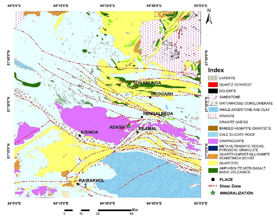
2. Study Area
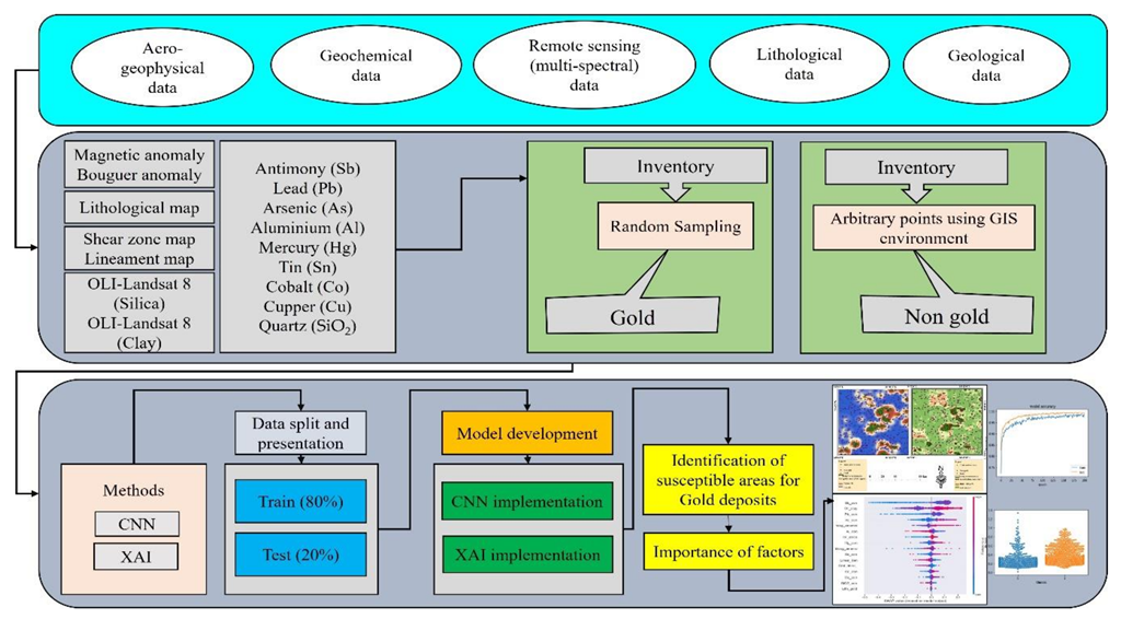
3. Data and Methodology
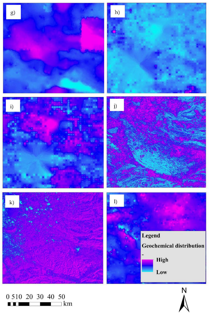
3.1. Detailed Description of Factors
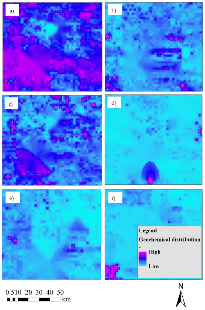
3.1.1. Geochemical Factors
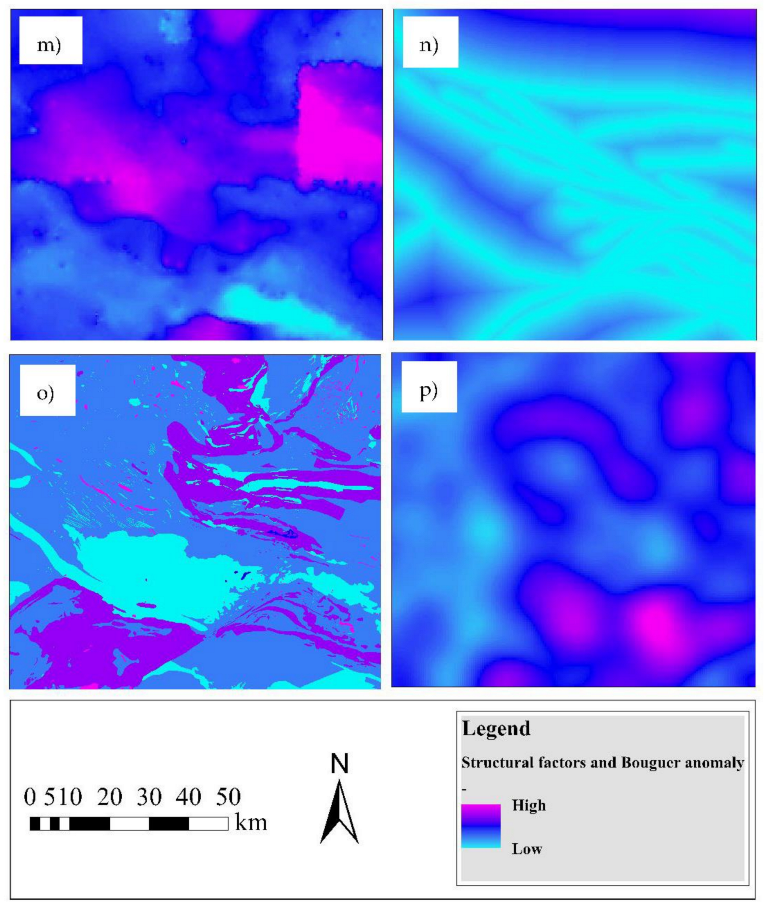
3.1.2. Geophysical Factors
3.1.3. Geological/Structural Factors
3.1.4. Mineralogical Factors
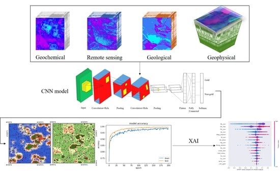
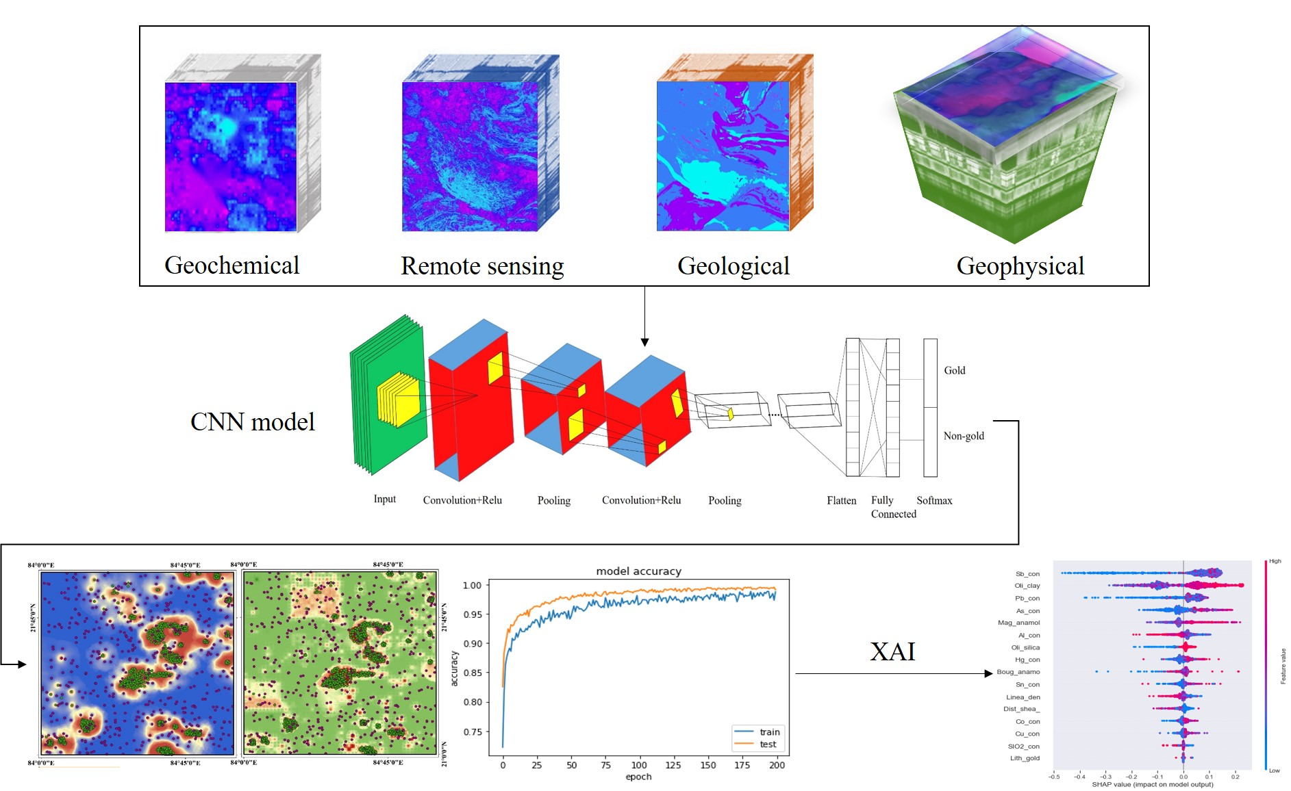
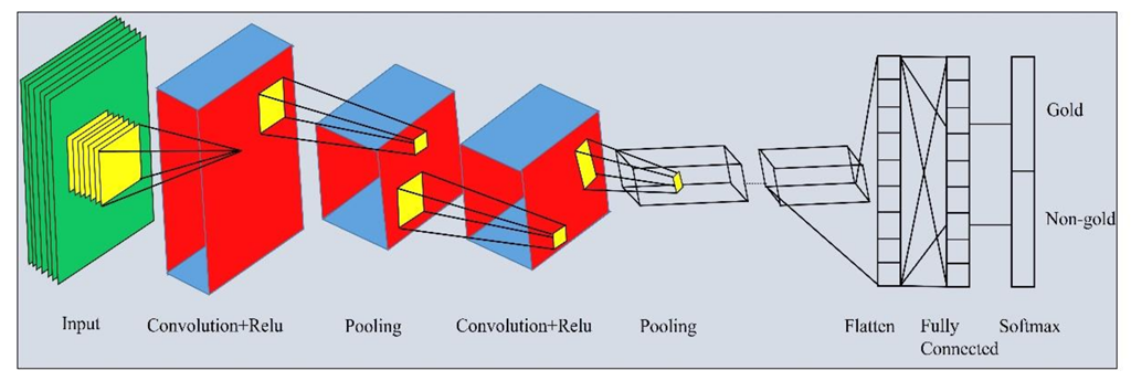
3.2. CNN
3.3. XAI Model
3.4. CNN Architecture and Implementation
3.5. Learning the Model Parameters and Performance
4. Results
5. Discussion
6. Conclusions
Author Contributions
Funding
Data Availability Statement
Conflicts of Interest
References
- Naqvi, S.M.; Naqvi, R.; Rogers, J.J.W. Precambrian Geology of India; Oxford University Press: New York, NY, USA, 1987. [Google Scholar]
- Knox-Robinson, C.M. Vectorial fuzzy logic: A novel technique for enhanced mineral prospectivity mapping, with reference to the orogenic gold mineralisation potential of the Kalgoorlie Terrane, Western Australia. Aust. J. Earth Sci. 2000, 47, 929–941. [Google Scholar] [CrossRef]
- Partington, G.A. Exploration targeting using GIS: More than a digital light table. In Proceedings of the Geo Computing Conference, Brisbane, Australia, 29 September–1 October 2010; Volume 51, pp. 83–89. [Google Scholar]
- Chung, C.F.; Agterberg, F.P. Regression models for estimating mineral resources from geological map data. J. Int. Assoc. Math. Geol. 1980, 12, 473–488. [Google Scholar] [CrossRef]
- Crowe, W.A.; Nash, C.R.; Harris, L.B.; Leeming, P.M.; Rankin, L.R. The geology of the Rengali Province: Implications for the tectonic development of northern Orissa, India. J. Asian Earth Sci. 2003, 21, 697–710. [Google Scholar] [CrossRef]
- Misra, S.; Gupta, S. Superposed deformation and inherited structures in an ancient dilational step-over zone: Post-mortem of the Rengali Province, India. J. Struct. Geol. 2014, 59, 1–17. [Google Scholar] [CrossRef]
- Banerji, A. Ore genesis and its relationship to volcanism, tectonism, granitic activity, and metasomatism along the Singhbhum shear zone, eastern India. Econ. Geol. 1981, 76, 905–912. [Google Scholar] [CrossRef]
- Ghosh, G.; Bose, S.; Das, K.; Dasgupta, A.; Yamamoto, T.; Hayasaka, Y.; Chakrabarti, K.; Mukhopadhyay, J. Transpression and juxtaposition of middle crust over upper crust forming a crustal scale flower structure: Insight from structural, fabric, and kinematic studies from the Rengali Province, eastern India. J. Struct. Geol. 2016, 83, 156–179. [Google Scholar] [CrossRef]
- Nash, C.; Rankin, L.; Leeming, P.; Harris, L. Delineation of lithostructural domains in northern Orissa (India) from Landsat Thematic Mapper imagery. Tectonophysics 1996, 260, 245–257. [Google Scholar] [CrossRef]
- Biswal, T.K.; De Waele, B.; Ahuja, H. Timing and dynamics of the juxtaposition of the Eastern Ghats Mobile Belt against the Bhandara Craton, India: A structural and zircon U-Pb SHRIMP study of the fold-thrust belt and associated nepheline syenite plutons. Tectonics 2007, 26, 1–21. [Google Scholar] [CrossRef]
- Ghosh, G.; Bose, S.; Guha, S.; Mukhopadhyay, J.; Aich, S. Remobilization of the southern margin of the Singhbhum Craton, eastern India during the Eastern Ghats orogeny. Indian J. Geol. 2010, 80, 97–114. [Google Scholar]
- Mahapatro, S.; Pant, N.; Bhowmik, S.; Tripathy, A.; Nanda, J. Archaean granulite facies metamorphism at the Singhbhum Craton–Eastern Ghats Mobile Belt interface: Implication for the Ur supercontinent assembly. Geol. J. 2012, 47, 312–333. [Google Scholar] [CrossRef]
- Carranza, E.J.M.; Hale, M. Geologically Constrained Probabilistic Mapping of Gold Potential, Baguio District, Philippines. Nat. Resour. Res. 2000, 9, 237–253. [Google Scholar] [CrossRef]
- An, P.; Moon, W.M.; Rencz, A.N. Application of fuzzy set theory to integrated mineral exploration. Can. J. Explor. Geophys. 1991, 27, 1–11. [Google Scholar]
- Eddy, B.G.; Bonham-Carter, G.F.; Jefferson, C.W. Mineral resource assessment of the Parry Islands, high Arctic, Canada: A GIS-base fuzzy logic model. In Proceedings of the Canadian Conference on GIS, Ottawa, ON, Canada, 4–10 June 1995. [Google Scholar]
- An, P.; Moon, W.M. An evidential reasoning structure for integrating geophysical, geological and remote sensing data. In Proceedings of the International Geoscience and Remote Sensing Symposium (IGARSS), Tokyo, Japan, 18–21 August 1993; pp. 1359–1361. [Google Scholar]
- Carranza, E.J.M. From Predictive Mapping of Mineral Prospectivity to Quantitative Estimation of Number of Undiscovered Prospects. Resour. Geol. 2011, 61, 30–51. [Google Scholar] [CrossRef]
- Carranza, E.J.M.; Hale, M. Evidential belief functions for data driven geologically constrained mapping of gold potential, Baguio district, Philippines. Ore Geol. Rev. 2002, 22, 117–132. [Google Scholar] [CrossRef]
- Carranza, E.J.M.; Woldai, T.; Chikambwe, E.M. Application of data driven evidential belief functions to prospectivity mapping for aquamarine-bearing pegmatites, Lundazi District, Zambia. Nat. Resour. Res. 2005, 14, 47–63. [Google Scholar] [CrossRef]
- Carranza, E.J.M.; Sadeghi, M. Predictive mapping of prospectivity and quantitative estimation of undiscovered VMS deposits in Skellefte district (Sweden). Ore Geol. Rev. 2010, 38, 219–241. [Google Scholar] [CrossRef]
- Carranza, E.J.M. Geochemical Anomaly and Mineral Prospectivity Mapping in GIS. Handbook of Exploration and Environmental Geochemistry; Elsevier: Amsterdam, The Netherlands, 2009; Volume 11. [Google Scholar]
- Bonham-Carter, G.F.; Agterberg, F.P.; Wright, D.F. Weights of evidence modeling: A new approach to mapping mineral potential. In Statistical Applications in the Earth Sciences; Agterberg, F.P., Bonham-Carter, G.F., Eds.; Geological Survey of Canada; Canadian Government Publishing Centre: Ottawa, ON, Canada, 1989; pp. 171–183. [Google Scholar]
- Carranza, E.J.M. Weights of evidence modeling of mineral potential: A case study using small number of prospects, Abra, Philippines. Nat. Resour. Res. 2004, 13, 173–187. [Google Scholar] [CrossRef]
- Austin, J.R.; Blenkinsop, T.G. Local to regional scale structural controls on mineralisation and the importance of a major lineament in the eastern Mount Isa In lier, Australia: Review and analysis with autocorrelation and weights of evidence. Ore Geol. Rev. 2009, 35, 298–316. [Google Scholar] [CrossRef]
- Arianne, F.; Craig, J.R.H. Mineral potential mapping in frontier regions: A Mongolian case study. Ore Geol. Rev. 2013, 51, 15–26. [Google Scholar]
- Oh, H.J.; Lee, S. Regional Probabilistic and Statistical Mineral Potential, Mapping of Gold-Silver Deposits Using GIS in the Gangreung Area, Korea. Resour. Geol. 2008, 58, 171–187. [Google Scholar] [CrossRef]
- Ernowo; Oktaviani, P. Regional probabilistic of gold-silver potential mapping using likelihood ratio models in Flores Island. In Proceedings of the 39th IAGI Annual Convention and Exhibition, Lombok, Indonesia, 22–25 November 2010. [Google Scholar]
- Carranza, E.J.M.; Hale, M.; Faassen, C. Selection of coherent deposit-type locations and their application in data-driven mineral prospectivity mapping. Ore Geol. Rev. 2008, 33, 536–558. [Google Scholar] [CrossRef]
- Singer, D.A.; Kouda, R. Application of a feed forward neural network in the search for Kuroko deposits in the Hokuroku District, Japan. Mathmatical Geol. 1996, 28, 1017–1023. [Google Scholar] [CrossRef]
- Oh, H.J.; Lee, S. Application of Artificial Neural Network for GoldSilver Deposits Potential Mapping: A Case Study of Korea. Nat. Resour. Res. 2011, 19, 103–124. [Google Scholar] [CrossRef]
- Surip, N.; Hamzah, A.H.; Zakaria, M.R.; Napiah, A.; Talib, J.A. Mapping of gold in densely vegetated area using remote sensing and GIS techniques in Pahang, Malaysia. In Proceeding of Asian Conference on Remote Sensing (ACRS), Kuala Lumpur, Malaysia, 12–16 November 2007. [Google Scholar]
- McMillan, M.; Haber, E.; Peters, B.; Fohring, J. Mineral prospectivity mapping using a VNet convolutional neural network. Lead. Edge 2021, 40, 99–105. [Google Scholar] [CrossRef]
- Xu, Y.; Li, Z.; Xie, Z.; Cai, H.; Niu, P.; Liu, H. Mineral prospectivity mapping by deep learning method in Yawan-Daqiao area, Gansu. Ore Geol. Rev. 2021, 138, 104316. [Google Scholar] [CrossRef]
- Ghosh, S.P.; Behere, S.N.; Mohanty, G. Report on the Exploration for Basemetals In the Extension Area of Adash Copper Prospect, Sambalpur District, Orissa; GSI Unpublished Report; Geological Survey of India: Kolkata, India, 1993. [Google Scholar]
- Ghosh Roy, A.K. Petrological Studies of The Mafic-Ultramafic Rocks Occurring Along the Contact Pegion Of Eastern Ghat Belt and Iron Ore Group in Parts of Sambalpur and Deogarh Districts, Orissa; Unpublished Interim Progress Report of Geological Survey of India; Geological Survey of India: Kolkata, India, 1998. [Google Scholar]
- Rana, G.; Rout, S.P.; Roychowdhury, K. Preliminary Investigation for Ree In the Contact Zone Between Eastern Ghats Mobile Belt and Singhbhum Craton Around Kankarkhol in Parts of Deogarh District, Odisha (UNFC Stage-G4); Unpublished Report of Geological Survey of India; Geological Survey of India: Kolkata, India, 2017. [Google Scholar]
- Rao, S.A.; Saha, T.K. Systematic Geological Mapping in Deogarh Sub- Division, Sambalpur Dist, Orissa; Unpublished Progress Report of Geological Survey of India; Geological Survey of India: Kolkata, India, 1972. [Google Scholar]
- Naskar, D.C.; Mukherjee, R.; Singh, A.K.; Kumar, A. Systematic geophysical mapping in parts of Angul, Sambalpur, Sundargarh and Deogarh districts of Odisha, to delineate subsurface structure. Richa Raghav Singh Prabodh Kumar Kushwaha SP Maurya Rohtash Kumar 2021, 25, 32–47. [Google Scholar]
- Talukdar, D.; Raul, A.K.; Gouda, H.C. Integration of Geological, Geochemical and Geophysical Data in Parts of Adash Area, Odisha with Limited Field-Check for the Search of Potential Mineral Blocks; Unpublished Report of Geological Survey of India; Geological Survey of India: Kolkata, India, 2019. [Google Scholar]
- Arrieta, A.B.; Díaz-Rodríguez, N.; Del Ser, J.; Bennetot, A.; Tabik, S.; Barbado, A.; García, S.; Gil-López, S.; Molina, D.; Benjamins, R. Explainable Artificial Intelligence (XAI): Concepts, taxonomies, opportunities and challenges toward responsible AI. Inf. Fusion 2020, 58, 82–115. [Google Scholar] [CrossRef]
- Dikshit, A.; Pradhan, B. Interpretable and explainable AI (XAI) model for spatial drought prediction. Sci. Total Environ. 2021, 801, 149797. [Google Scholar] [CrossRef]
- Behera, S.; Panigrahi, M.K.; Pradhan, A. Identification of geochemical anomaly and gold potential mapping in the Sonakhan Greenstone belt, Central India: An integrated concentration-area fractal and fuzzy AHP approach. Appl. Geochem. 2019, 107, 45–57. [Google Scholar] [CrossRef]
- Zhang, N.; Zhou, K.; Li, D. Back-propagation neural network and support vector machines for gold mineral prospectivity mapping in the Hatu region, Xinjiang, China. Earth Sci. Inform. 2018, 11, 553–566. [Google Scholar] [CrossRef]
- Raines, G.L. Evaluation of weights of evidence to predict epithermal-gold deposits in the Great Basin of the Western United States. Nat. Resour. Res. 1999, 8, 257–276. [Google Scholar] [CrossRef]
- Bonham-Carter, G.F.; Agterberg, F.P.; Wright, D.F. Integration of geological datasets for gold exploration in Nova Scotia. Photogramm. Eng. Remote Sens. 1998, 54, 1585–1592. [Google Scholar]
- Dasgupta, A.; Bose, S.; Das, K.; Ghosh, G. Petrological and geochemical evolution of the Central Gneissic Belt, Rengali Province, eastern India: Implications for the Neoarchean growth and orogenesis. J. Asian Earth Sci. 2017, 146, 1–19. [Google Scholar] [CrossRef]
- Ghosh, G.; Bose, S. Deformation and metamorphic history of the Singhbhum Craton vis–à–vis peripheral mobile belts, eastern India: Implications on Precambrian crustal processes. J. Mineral. Petrol. Sci. 2020, 115, 70–87. [Google Scholar] [CrossRef]
- Saha, A.K. Crustal Evolution of Singhbhum North Orissa Eastern India. In Memorendum of Geological Society of India; Geological Survey of India: Kolkata, India, 1994. [Google Scholar]
- Panda, P.K.; Patra, P.C.; Nanda, J.K. Petrochemistry of the alkaline rocks of Rairakhol–Kankarakhol belt, Sambalpur and Deogarh districts, Orissa. Geol. Surv. India Spec. Publ. 1998, 44, 307–314. [Google Scholar]
- Panda, P.K.; Patra, P.C.; Patra, R.N.; Nanda, J.K. Nepheline syenite from Rairakhol, Sambalpur district, Orissa. J. Geol. Soc. India 1993, 41, 144–151. [Google Scholar]
- Ranjan, S.; Upadhyay, D.; Abhinay, K.; Pruseth, K.L.; Nanda, J.K. Zircon geochronology of deformed alkaline rocks along the Eastern Ghats Belt margin: India–Antarctica connection and the Enderbia continent. Precambrian Res. 2018, 310, 407–424. [Google Scholar] [CrossRef]
- Sheikh, J.M.; Patel, S.C.; Champati, A.K.; Madhavan, K.; Behera, D.; Naik, A.; Gerdes, A. Nepheline syenite intrusions from the Rengali Province, eastern India: Integrating geological setting, microstructures, and geochronological observations on their syntectonic emplacement. Precambrian Res. 2020, 346, 105802. [Google Scholar] [CrossRef]
- Ganguly, P.K.; De, S.K.; Chattopadhyay, R.C. Report on the test geophysical investigations for sulphide mineralisation near Medinipur-Budido villages, Sambalpur district, Orissa; (unpublished progress report for the F.S. 1974–1975); Geological Survey of India: Kolkata, India, 1975. [Google Scholar]
- Karim, M.A.; Hussain, A.; Mohanty, S.N. Interim Report on The Regional Geochemical Survey in Deogarh Greenstone Belt for Assessing Economic Mineral Potential; unpublished interim report; Geological Survey of India: Kolkata, India, 2011. [Google Scholar]
- Ahmadirouhani R, Karimpour M-H, Rahimi B, Malekzadeh-Shafaroudi A, Pour AB, Pradhan B Integration of SPOT-5 and ASTER satellite data for structural tracing and hydrothermal alteration mineral mapping: Implications for Cu–Au prospecting. Int. J. Image Data Fusion 2018, 9, 237–262. [CrossRef]
- Bhukosh Portal, Geological Survey of India. Available online: https://bhukosh.gsi.gov.in/Bhukosh/Public (accessed on 10 July 2021).
- Sun, T.; Chen, F.; Zhong, L.; Liu, W.; Wang, Y. GIS-based mineral prospectivity mapping using machine learning methods: A case study from Tongling ore district, eastern China. Ore Geol. Rev. 2019, 109, 26–49. [Google Scholar] [CrossRef]
- Sheikhrahimi, A.; Pour, A.B.; Pradhan, B.; Zoheir, B. Mapping hydrothermal alteration zones and lineaments associated with orogenic gold mineralization using ASTER data: A case study from the Sanandaj-Sirjan Zone, Iran. Adv. Space Res. 2019, 63, 3315–3332. [Google Scholar] [CrossRef]
- Wang, G.; Pang, Z.; Boisvert, J.B.; Hao, Y.; Cao, Y.; Qu, J. Quantitative assessment of mineral resources by combining geostatistics and fractal methods in the Tongshan porphyry Cu deposit (China). J. Geochem. Explor. 2013, 134, 85–98. [Google Scholar] [CrossRef]
- Kashani, S.B.M.; Abedi, M.; Norouzi, G.-H. Fuzzy logic mineral potential mapping for copper exploration using multi-disciplinary geo-datasets, a case study in seridune deposit, Iran. Earth Sci. Inform. 2016, 9, 167–181. [Google Scholar] [CrossRef]
- Motta, J.G.; Faria, I.R. A mineral potential mapping approach for supergene nickel deposits in southwestern São Francisco Craton, Brazil. Braz. J. Geol. 2016, 46, 261–273. [Google Scholar] [CrossRef]
- Chung, C.-J.; Keating, P.B. Mineral potential evaluation based on airborne geophysical data. Explor. Geophys. 2002, 33, 28–34. [Google Scholar] [CrossRef]
- Porwal, A.; Carranza, E.; Hale, M. Knowledge-driven and data-driven fuzzy models for predictive mineral potential mapping. Nat. Resour. Res. 2003, 12, 1–25. [Google Scholar] [CrossRef]
- Dentith, M.; Mudge, S.T. Geophysics for the Mineral Exploration Geoscientist; Cambridge University Press: Cambridge, UK, 2014. [Google Scholar]
- Moreira, C.A.; Ilha, L.M. Prospecção geofísica em ocorrência de cobre localizada na bacia sedimentar do Camaquã (RS). Rem Rev. Esc. De Minas 2011, 64, 305–311. [Google Scholar] [CrossRef] [Green Version]
- Doyle, H. Geophysical exploration for gold? A review. Explor. Geophys. 1986, 17, 169–180. [Google Scholar] [CrossRef]
- Foster, B. Gold Metallogeny and Exploration; Springer: Dordrecht, The Netherlands, 1993; 432p. [Google Scholar]
- Bolouki, S.M.; Ramazi, H.R.; Maghsoudi, A.; Beiranvand Pour, A.; Sohrabi, G. A remote sensing-based application of bayesian networks for epithermal gold potential mapping in Ahar-Arasbaran area, NW Iran. Remote Sens. 2020, 12, 105. [Google Scholar] [CrossRef]
- Van der Meer, F.D.; Van der Werff, H.M.; Van Ruitenbeek, F.J.; Hecker, C.A.; Bakker, W.H.; Noomen, M.F.; Van Der Meijde, M.; Carranza, E.J.M.; De Smeth, J.B.; Woldai, T. Multi-and hyperspectral geologic remote sensing: A review. Int. J. Appl. Earth Obs. Geoinf. 2012, 14, 112–128. [Google Scholar] [CrossRef]
- LeCun, Y.; Bottou, L.; Bengio, Y.; Haffner, P. Gradient-based learning applied to document recognition. Proc. IEEE 1998, 86, 2278–2324. [Google Scholar] [CrossRef]
- Krizhevsky, A.; Sutskever, I.; Hinton, G.E. Imagenet classification with deep convolutional neural networks. Adv. Neural Inf. Processing Syst. 2012, 25, 1097–1105. [Google Scholar] [CrossRef]
- Kingma, D.P.; Ba, J. Adam: A method for stochastic optimization. arXiv 2014, arXiv:1412.6980. [Google Scholar]
- Lundberg, S.M.; Lee, S.-I. A unified approach to interpreting model predictions. In Proceedings of the 31st International Conference on Neural Information Processing Systems, Long Beach, CA, USA, 4–9 December 2017; pp. 4768–4777. [Google Scholar]
- Mitchell, A. TM Machine Learning in Ecosystem Informatics and Sustainability; McGraw-Hill Science/Engineering/Math: New York, NY, USA, 1997. [Google Scholar]
- Severyn, A.; Moschitti, A. Unitn: Training deep convolutional neural network for twitter sentiment classification. In Proceedings of the 9th International Workshop on Semantic Evaluation (SemEval 2015), Denver, CA, USA, 4–5 June 2015; pp. 464–469. [Google Scholar]
- Zhao, S.; Guo, Y.; Sheng, Q.; Shyr, Y. Advanced heat map and clustering analysis using heatmap3. BioMed Res. Int. 2014, 2014, 986048. [Google Scholar] [CrossRef] [PubMed]
- Chakravarti, R.; Singh, S.; Venkatesh, A.; Patel, K.; Sahoo, P. A modified placer origin for refractory gold mineralization within the Archean radioactive quartz-pebble conglomerates from the eastern part of the Singhbhum Craton, India. Econ. Geol. 2018, 113, 579–596. [Google Scholar] [CrossRef]
- Singh, S.; Chakravarti, R.; Barla, A.; Behera, R.C.; Neogi, S. A holistic approach on the gold metallogeny of the Singhbhum crustal province: Implications from tectono-metamorphic events during the Archean-Proterozoic regime. Precambrian Res. 2021, 365, 106376. [Google Scholar] [CrossRef]
- Macdonald, E. Handbook of Gold Exploration and Evaluation; Elsevier: Amsterdam, The Netherlands, 2007. [Google Scholar]
- Goldfarb, R.J.; Groves, D.I.; Gardoll, S. Orogenic gold and geologic time: A global synthesis. Ore Geol. Rev. 2001, 18, 1–75. [Google Scholar] [CrossRef]
- Goldfarb, R.; Baker, T.; Dubé, B.; Groves, D.I.; Hart, C.J.; Gosselin, P. Distribution, Character and Genesis of Gold Deposits in Metamorphic Terranes; Society of Economic Geologists: Littleton, CO, USA, 2005. [Google Scholar]
- Goldfarb, R.J.; Groves, D.I. Orogenic gold: Common or evolving fluid and metal sources through time. Lithos 2015, 233, 2–26. [Google Scholar] [CrossRef]
- Biswas, S. Geological Setup for Gold Prospects and Deposits in India. Conf. GSI 2021, 1–13. [Google Scholar] [CrossRef]
- Sui, J. Geochronology and Genesis of the Zaozigou Gold Deposit, Gansu Province, China. Ph.D. Thesis, China University of Geosciences, Wuhan, China, 2012. (In Chinese with English Abstract). [Google Scholar]
- Zhang, S.; Carranza, E.J.M.; Wei, H.; Xiao, K.; Yang, F.; Xiang, J.; Zhang, S.; Xu, Y. Data-driven mineral prospectivity mapping by joint application of unsupervised convolutional auto-encoder network and supervised convolutional neural network. Nat. Resour. Res. 2021, 30, 1011–1031. [Google Scholar] [CrossRef]


| Factors | Code Names | Sources | Resolution and Scale | References |
|---|---|---|---|---|
| Magnetic anomaly Bouguer anomaly | Mag_anamol Boug_anamol | Crowe et al. [5]; Nash et al. [9]; BHUKOSH portal, Geological map of India [56] | 25 m and 1:50 k | The importance of all the factors mentioned are chosen based on gold group elements (gold, silver, copper, mercury, aluminium and lead) [55,57,58] |
| Antimony (Sb) Lead (Pb) Arsenic (As) Aluminium (Al) Mercury (Hg) Tin (Sn) Cobalt (Co) Cupper (Cu) Quartz (SiO2) | Sb_con Pb_con As_con Al_con Hg_con Sn_con Co_con Cu_con SIO2_con | |||
| Lithological map Shear zone Lineament map | Lith_gold Dist_shear Linea_den | |||
| OLI-Landsat 8 (silica) OLI-Landsat 8 (clay) | Oli_silica Oli_clay | United States Geological Survey (USGS) |
| Layer (Type) | Output Shape | No. of Parameters |
|---|---|---|
| dense_1 (dense) | (None, 200) | 3400 |
| dropout_1 (dropout) | (None, 200) | 0 |
| dense_2 (dense) | (None, 200) | 40200 |
| dropout_2 (dropout) | (None, 200) | 0 |
| dense_3 (dense) | (None, 200) | 40200 |
| dropout_3 (dropout) | (None, 200) | 0 |
| dense_4 (dense) | (None, 200) | 40200 |
| dropout_4 (dropout) | (None, 200) | 0 |
| dense_5 (dense) | (None, 2) | 402 |
| Total parameters: 124,402 | ||
| Trainable parameters: 124,402 | ||
| Non-trainable parameters: 0 | ||
| Actual | Predicted | ||
| Positive | Negative | ||
| Positive | 81 | 19 | |
| Negative | 7 | 174 | |
| Major Concentrations | Minimum | Maximum | Sum | Mean | Standard Deviation |
|---|---|---|---|---|---|
| Au_con (ppb) | 1.42 | 410 | 48743.52 | 34.72 | 47.96 |
| Sb_con (ppm) | 0.015 | 1.34 | 475.45 | 0.34 | 0.18 |
| Pb_con (ppm) | 2.63 | 81.29 | 35039.13 | 24.96 | 11.85 |
| As_con (ppm) | 1.13 | 82.08 | 12491.84 | 8.90 | 7.79 |
| Precision | Recall | F1-Score | Support | |
|---|---|---|---|---|
| Non-gold | 0.92 | 0.81 | 0.86 | 100 |
| Gold | 0.90 | 0.96 | 0.93 | 181 |
| Accuracy | 0.91 | 281 | ||
| Macro-average | 0.91 | 0.89 | 0.90 | 281 |
| Weighted average | 0.91 | 0.91 | 0.91 | 281 |
| Classification accuracy: 0.90 | ||||
Publisher’s Note: MDPI stays neutral with regard to jurisdictional claims in published maps and institutional affiliations. |
© 2022 by the authors. Licensee MDPI, Basel, Switzerland. This article is an open access article distributed under the terms and conditions of the Creative Commons Attribution (CC BY) license (https://creativecommons.org/licenses/by/4.0/).
Share and Cite
Pradhan, B.; Jena, R.; Talukdar, D.; Mohanty, M.; Sahu, B.K.; Raul, A.K.; Abdul Maulud, K.N. A New Method to Evaluate Gold Mineralisation-Potential Mapping Using Deep Learning and an Explainable Artificial Intelligence (XAI) Model. Remote Sens. 2022, 14, 4486. https://doi.org/10.3390/rs14184486
Pradhan B, Jena R, Talukdar D, Mohanty M, Sahu BK, Raul AK, Abdul Maulud KN. A New Method to Evaluate Gold Mineralisation-Potential Mapping Using Deep Learning and an Explainable Artificial Intelligence (XAI) Model. Remote Sensing. 2022; 14(18):4486. https://doi.org/10.3390/rs14184486
Chicago/Turabian StylePradhan, Biswajeet, Ratiranjan Jena, Debojit Talukdar, Manoranjan Mohanty, Bijay Kumar Sahu, Ashish Kumar Raul, and Khairul Nizam Abdul Maulud. 2022. "A New Method to Evaluate Gold Mineralisation-Potential Mapping Using Deep Learning and an Explainable Artificial Intelligence (XAI) Model" Remote Sensing 14, no. 18: 4486. https://doi.org/10.3390/rs14184486