Synchronous Atmospheric Correction of High Spatial Resolution Images from Gao Fen Duo Mo Satellite

Abstract

Atmospheric conditions vary significantly in terms of the temporal and spatial scales. Therefore, it is critical to obtain atmospheric parameters synchronized with an image for atmospheric correction based on radiative transfer calculation methods. On 3 July 2020, the high resolution and multimode imaging satellite, Gao Fen Duo Mo (GFDM), which was the first civilian high-resolution remote sensing satellite equipped with the Synchronization Monitoring Atmospheric Corrector (SMAC), was launched. The SMAC is a multispectral and polarization detection device that is used to retrieve atmospheric parameters that are time-synchronized with the image sensor of GFDM in the same field-of-view. On the basis of the atmospheric parameters obtained from the SMAC, a synchronization atmospheric correction (Syn-AC) method is proposed to remove the influence of the atmosphere and the adjacency effects to retrieve the surface reflectance. The Syn-AC method was applied in the experiments of synchronous atmospheric correction for GFDM images, where the surface reflectance retrieved via the Syn-AC method was compared with the field-measured values. In addition, the classical correction method, the FLAASH, was applied in the experiments to compare its performance with that of the Syn-AC method. The results indicated that the image possessed better clarity and contrast with the blurring effect removed, and the multispectral reflectance was in agreement with the field-measured spectral reflectance. The deviations between the reflectance retrievals of Syn-AC and the field-measured values of the selected targets were within 0.0625, representing a higher precision than that of the FLAASH method (the max deviation was 0.2063). For the three sites, the mean relative error of Syn-AC was 19.3%, and the mean relative error of FLAASH was 76.6%. Atmospheric correction based on synchronous atmospheric parameters can improve the quantitative accuracy of remote sensing images, and it is meaningful for remote sensing applications.

1. Introduction

During optical satellite imaging of the Earth, the observed radiance of a satellite sensor is mainly influenced by three aspects: the illumination, observation geometry, and interaction between solar radiation with the atmosphere and ground surface [1]. The scattering and absorption of molecules and aerosols play a significant role in the radiation extinction [2]. In addition, the interference contribution of the surrounding pixels is a major cause of blurred visual effects of images, called the adjacency effect [3]. The purpose of atmospheric correction (AC) is to reduce the influence of the atmosphere and adjacency effects to retrieve the real reflectance of ground objects for high spatial resolution satellite imagery [4]. Atmospheric parameters, such as aerosol optical depth (AOD) and column water vapor (CWV), are key factors affecting the quantitative estimation of the influence of atmospheric radiation. However, atmospheric conditions vary significantly in terms of temporal and spatial scales [5]. Therefore, synchronous acquisition of atmospheric parameters is important. Several efforts have been made to obtain atmospheric parameters that are synchronized with the space-time of the image to be corrected, and currently, three kinds of approaches are available.

In the first method, the atmospheric parameters are measured using ground-based technologies, such as the Aerosol Robotic Network (AERONET) [6]. However, ground-based data solely represent the atmospheric conditions restricted to the observation site area and cannot be applied for large-scale spatial analyses [7]. In the second method, the spectral information of the sensor such as the Moderate-resolution Imaging Spectroradiometer (MODIS) is used for aerosol retrieval [8]. However, the ground sample distance of these aerosol retrieval products is greater than 10 km, and the accuracy of aerosol retrieval products with higher spatial resolution should be further improved [9]. Furthermore, sensors with high-spatial resolution are used to obtain detailed ground information, though generally, their imaging bandwidth is relatively wide, which is insufficient for atmospheric detection [7].

In the third method, the atmospheric parameters for atmospheric correction are simultaneously measured by an instrument, which is equipped on the platform of a satellite. This method can solve the spatial and temporal matching between atmospheric parameters and images, and improve the accuracy of the parameters, which has been a development direction in recent years for remote sensing with high spatial resolution [10].

On 21 November 2000, the Earth Observing-1 (EO-1) satellite was launched successfully by the National Aeronautics and Space Administration (NASA). The satellite platform was equipped with a Linear Etalon Imaging Spectrometer Array (LEISA) Atmospheric Corrector (LAC) for the atmospheric correction of the multispectral imagery from the Advanced Land Imager (ALI) [11]. In August 2014, a commercial US company (DigitalGlobe) launched the WorldView-3 satellite, which was equipped with an instrument to detect atmospheric conditions [12]. The Clouds, Aerosols, water Vapor, Ice, and Snow (CAVIS) sensor covers 12 wavelength bands ranging from 405 nm (ultraviolet) to 2245 nm (short-wave infrared) with a spatial resolution of approximately 30 m. Atmospheric correction can be performed based on the atmospheric parameters from CAVIS for the high resolution remote sensing images of the WorldView-3 satellite [11].

On 3 July 2020, the China National Space Administration (CNSA) launched the high- resolution and multimode imaging satellite, Gao Fen Duo Mo (GFDM). The main imaging sensor onboard the satellite is configured with 1 panchromatic and 8 multispectral bands, and the spatial resolutions are 0.42 m and 1.6 m, respectively. In addition, the platform is also equipped with the Synchronization Monitoring Atmospheric Corrector (SMAC) to detect atmospheric parameters. The SMAC can offer atmospheric measurements that are time-synchronized with the image sensor of GFDM in the same field-of-view for synchronous atmospheric correction. The SMAC equipment was developed by the Anhui Institute of Optics and Fine Mechanics, Hefei Institutes of Physical Science, Chinese Academy of Sciences (CAS).

In this study, a synchronous atmospheric correction (Syn-AC) method is proposed based on the SMAC. First, the data processing procedures of the SMAC are detailed. Then, a brief introduction of the atmospheric parameters inversion methods based on the SMAC is presented. Third, the main principles of the atmospheric correction method based on synchronous atmospheric parameters provided by the SMAC are stated. To evaluate the performance of Syn-AC, six images under different atmospheric conditions, which are from three radiometric calibration sites [13,14,15] (Dunhuang, Songshan, and Baotou) were selected to conduct atmospheric correction experiments. Then, the visual effects before and after AC were compared. In addition, the average reflectance of the selected targets in the surface reflectance image of Syn-AC was compared with the field-measured reflectance for evaluating the performance of correction methods, as well as the evaluation of fast line-of-sight atmospheric analysis of spectral hypercubes (FLAASH). Finally, the performance of Syn-AC and FLAASH were compared.

2. Satellite and Equipment

2.1. The GFDM Satellite

The GFDM satellite operates in a Sun-synchronous orbit with an orbital altitude of 643.8 km and a global average revisit period of less than 2 days [16]. The detailed parameters are listed in

Table 1. Parameters of GFDM satellite.

Satellite	Type	Sun-synchronous circular orbit
	Orbit altitude	643.8 km
	Revisit	less than 2 days
High Resolution Camera	Swath Width	≥15 km
	Resolution	Panchromatic: 0.42 m; Multispectral: 1.6 m
Band Setting /nm	pan	450–900
	band 1	450–520
	band 2	520–590
	band 3	630–690
	band 4	770–890
	band 5	400–450
	band 6	590–625
	band 7	705–745
	band 8	860–1040

. The spectral response function of GFDM satellite is depicted in Figure 1. The GFDM satellite is equipped with a high-resolution optical camera, an atmospheric synchronization corrector, and auxiliary equipment [17]. As the first scientific optical remote sensing civilian satellite with submeter-scale resolution in China [16], the spatial resolution of a panchromatic band and 8 multispectral bands are 0.42 m and 1.6 m at the nadir, respectively. In addition, considering the high performance of this agile platform and its multiple imaging modes, the GFDM satellite can accurately and efficiently acquire satellite images, with large data volumes expected to be widely used in surveying and mapping, agriculture, and other industries to further meet the demand of high precision data for emergency management, disaster mitigation, and monitoring of construction activities and natural resources [18].

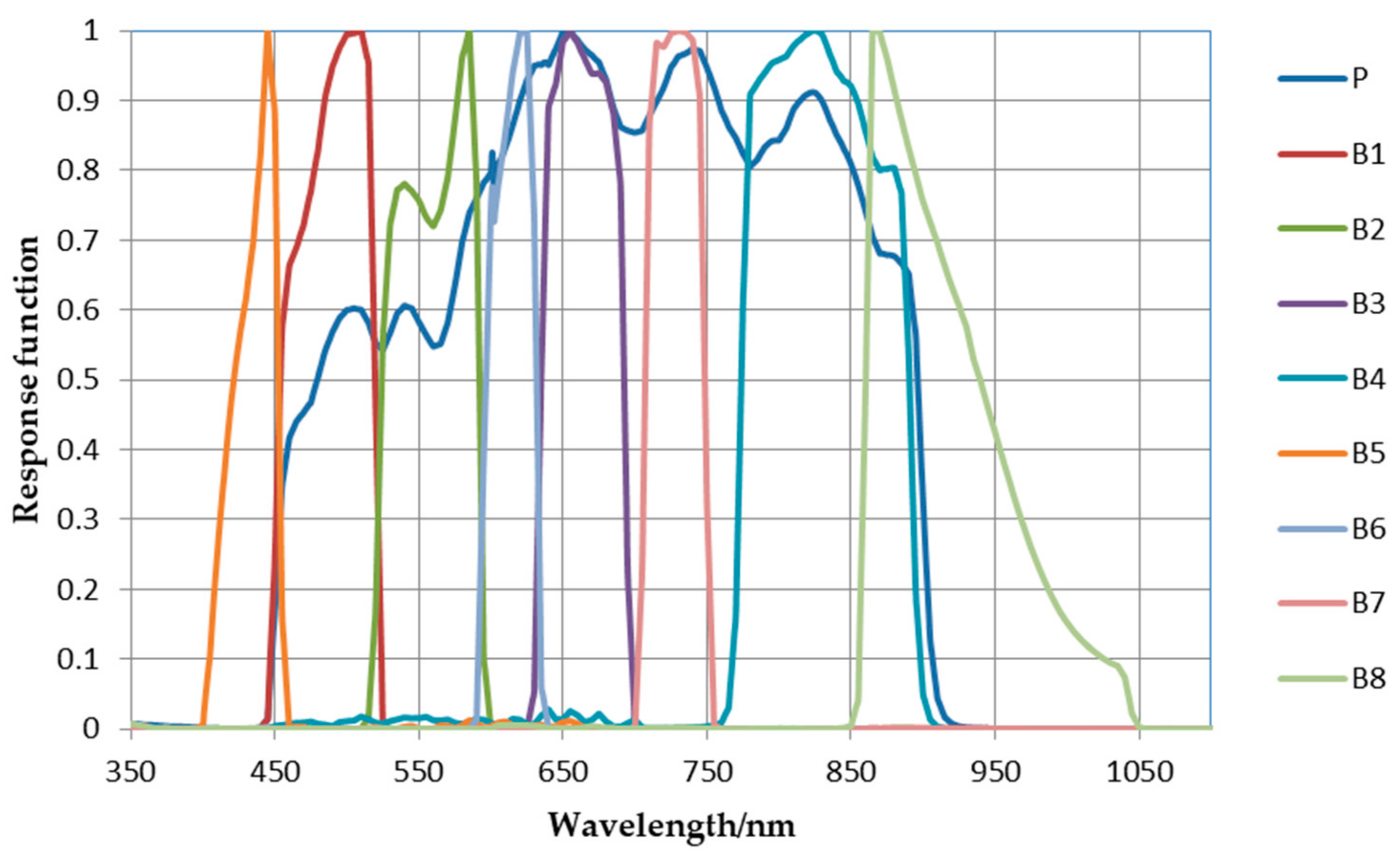
2.2. The SMAC Equipment

The SMAC onboard the GFDM satellite platform is capable of multispectral and polarization detection and can record atmospheric observations on the surface to obtain atmospheric parameters that are synchronized with the main image sensor [16]. The configuration details of the SMAC are presented in

Table 2. Settings of SMAC equipment.

Spatial resolution	6.7 km	Polarizer orientation	0°, 60°, 120° (490, 670, 870, 1610 nm) 0°, 60°, 120°, 145° (2250 nm)
Instrument FOV	1.48°	Band width	20, 20, 20, 40, 20, 40, 60, 80 nm
Swath width	2 pixels	Rad. Cal. Error	≤5% (490, 550, 670, 870, 910 nm) ≤6% (1380, 1610, 2250 nm)
Imaging	No	Pol. Cal. Error	≤0.01 (DOLP ≥ 0.02)
Band/nm		Observation mission
490 P		Aerosol and Clouds
550		Aerosol and Clouds
670 P		Aerosol and Clouds
870 P		Aerosol and Water vapor
910		Water vapor
1380		Cirrus
1610 P		Aerosol and Surface
2250 P		Aerosol and Surface

DOLP Degree of linear polarization; ^P Bands with polarization.

. The SMAC operates over eight wavelength bands, ranging from 490 nm (visible) to 2250 nm (short-wave infrared), with a spatial resolution of approximately 6.7 km. Five polarized bands of SMAC are centered at 490, 670, 870, 1610, and 2250 nm, and marked with superscript P in Table 2. During synchronous observation, the detection of different atmospheric parameters were accomplished based on spectrum and polarization information from different wavelengths.

To achieve the simultaneous measurement of each polarized channel, the SMAC equipment utilizes a split-aperture detection method, and each channel adopts a dual pixel shooting mode [19]. The synchronous detection mode is depicted in Figure 2. In Figure 2a, the arrow denotes the flight direction of the GFDM satellite. The SMAC measurements are indicated by the two square pixels corresponding to the dual detector. For detecting the covered spatial area, the SMAC starts up before and shuts down after the main CCD. Therefore, in Figure 2b, the golden-filled boxes cover a larger area than the entire image during one observation, and the breadth of the two box pixels is slightly larger than the image width. The central longitude and latitude of the two pixels are represented by the green dotted lines. In addition, because the SMAC performs intensive shooting with a frequency of 10 times per second, the green dotted lines form redundant along-tracks, as illustrated in Figure 2b.

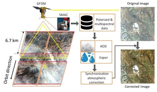
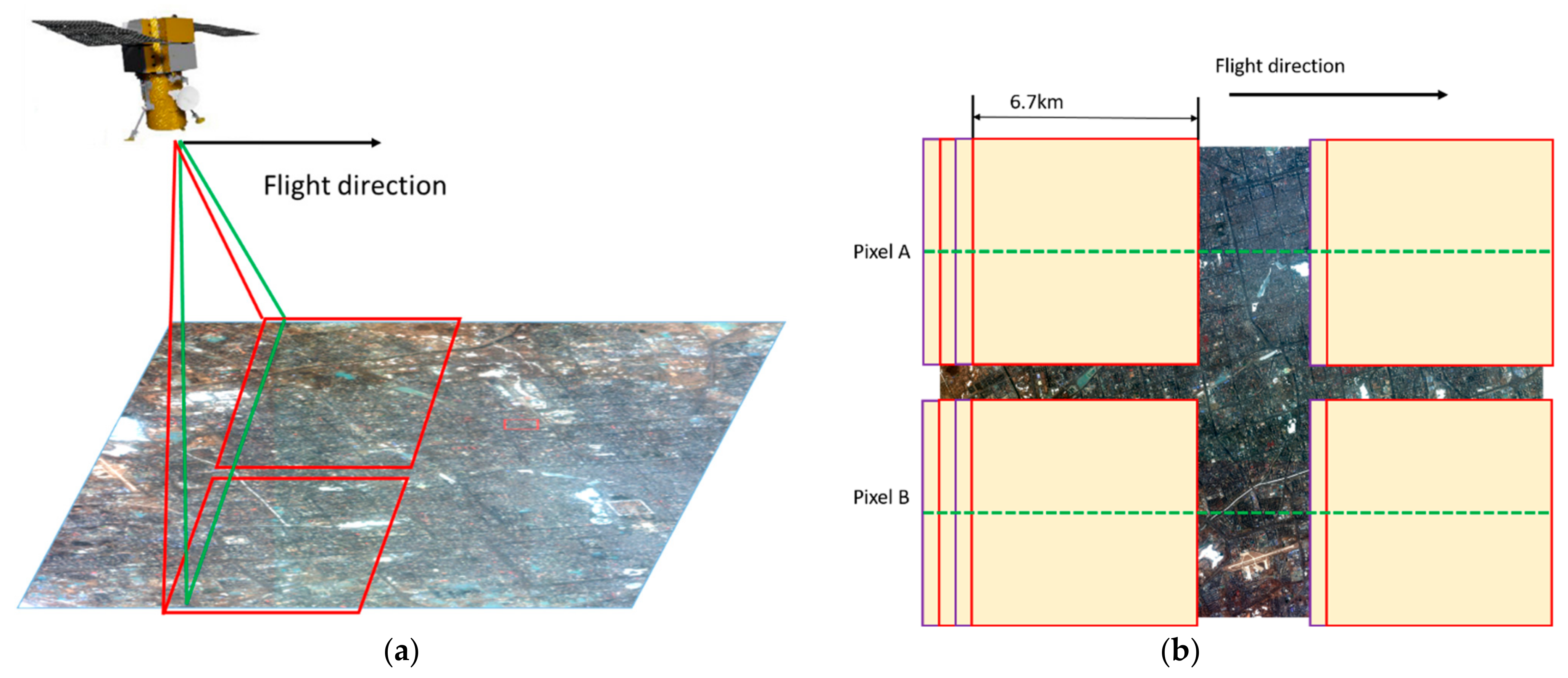
3. Atmospheric Synchronization Correction Method Based on the SMAC

The main ideas proposed in the developed synchronization atmospheric correction technique are presented in this section, including data processing steps for the SMAC, brief techniques of atmospheric parameter inversion, and principles of atmospheric synchronization correction.

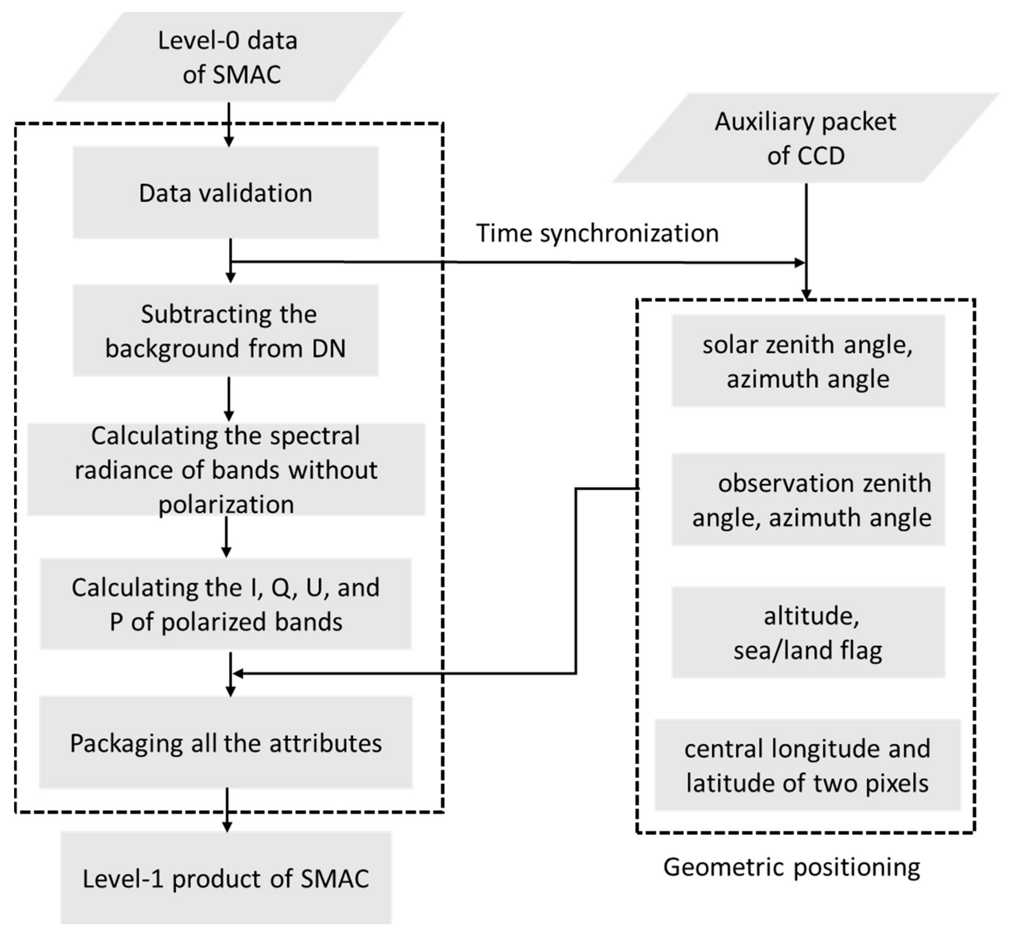
3.1. Data Processing for SMAC

Synchronized with the auxiliary data of the main CCD, the raw data of the SMAC, called Level-0 data, comprise digital number (DN) values stored in frames, and the size of one frame is 930 bytes, which are obtained through consecutive observations per second. The raw data are used as an input for data processing and processed following the steps illustrated in Figure 3, to invert atmospheric parameters in the subsequent step.

First, to ensure the validity of all of the retained data, data validation is conducted to check for anomalous attributes, for example, the working mode (observation or holding state) and temperature of the detector.

In step 2, according to the current temperature of the detector, the background under the heat sink temperatures obtained from the calibration profile is calculated via linear interpolation and subtracted from the DN.

In step 3, the spectral radiance of each band without polarization (550, 910, and 1380 nm) is calculated as

$$L_{\lambda }=\frac{D{N}_{\lambda }}{A_{\lambda }\ast Z_{\lambda }},$$

(1)

where $\lambda$ denotes the band, $A_{\lambda }$ and $Z_{\lambda }$ refer to the absolute spectral response and gain of each band, respectively. The radiance unit is equal to ${\mathsf{\mu }\mathrm{W}\mathrm{cm}}^{-2}{\mathrm{nm}}^{-1}{\mathrm{sr}}^{-1}$.

In step 4, considering the polarized bands (490, 670, 870, 1610, and 2250 nm), combined with the calibration data, the Stokes parameters including $I$, $Q$, and $U$ are expressed [20] as

$$\left[\begin{array}{c}{I}_{\lambda }\\ Q_{\lambda }\\ U_{\lambda }\end{array}\right]=\frac{1}{A_{\lambda ,2}\ast Z_{\lambda ,2}}{\left[\begin{array}{ccc}\begin{array}{c}1\\ 1\\ 1\end{array}& \begin{array}{c}cos\left(2\left({\alpha }_{\lambda }+{\alpha }_{\lambda ,1}\right)\right)\\ cos\left(2({\alpha }_{\lambda }+{\alpha }_{\lambda ,2})\right)\\ cos\left(2({\alpha }_{\lambda }+{\alpha }_{\lambda ,3})\right)\end{array}& \begin{array}{c}-sin\left(2\left({\alpha }_{\lambda }+{\alpha }_{\lambda ,1}\right)\right)\\ -sin\left(2({\alpha }_{\lambda }+{\alpha }_{\lambda ,2})\right)\\ -sin\left(2({\alpha }_{\lambda }+{\alpha }_{\lambda ,3})\right)\end{array}\end{array}\right]}^{-1}\left[\begin{array}{c}D{N}_{\lambda ,1}/T_{\lambda ,1}\\ D{N}_{\lambda ,2}\\ D{N}_{\lambda ,3}/T_{\lambda ,3}\end{array}\right]$$

(2)

where $i$ denotes the channels with different polarization angles, as mentioned in Table 2, $D{N}_{\lambda ,i}$, ${\alpha }_{\lambda ,i}$ and $T_{\lambda ,i}$ represent the DN value, polarization orientation angle, and relative transmittance for band $\lambda$ and channel $i$, respectively. Polarized detection is relatively more sensitive to atmosphere, and the retrieval of aerosol parameters can benefit from this sensitivity as a result [21,22,23,24]. Furthermore, the degree of polarization $P_{\lambda }$ can be calculated as

$$P_{\lambda }=\frac{\sqrt{{(Q_{\lambda })}^2+{(U_{\lambda })}^2}}{I_{\lambda }}.$$

(3)

Step 5 involves the satellite geometric positioning. Based on the principle of time synchronization, geometric data, including the zenith and azimuth angles of the Sun and the SMAC sensor, the sea/land flag and altitude, and the central longitude and latitude of the two pixels of SMAC, are calculated via a combination with the auxiliary data packets of the CCD provided by the satellite platform.

Finally, the Level-0 data of the SMAC are processed in a time sequence to obtain the Level-1 product of the SMAC. As shown in

Table 3. Level-1 product of SMAC.

Parameter	Instruction	Parameter	Instruction
Identification of SMAC data	1 column; Filled with 0 × 62;	Sea-land flag	1 column for each pixel (A and B); 0-Sea;1-Land
Package number	1 column; Filled with C000~FFFFH	Altitude	1 column for each pixel (A and B)
Latitude and longitude	2 columns for each pixel (A and B);	Time stamp	1 column; Coordinated universal time
Solar zenith angle and azimuth angle	2 columns;	I, Q, U, and P of polarized bands	4 columns for each pixel (A and B); 20 columns in total
Viewing zenith angle and azimuth angle	2 columns for each pixel (A and B);	Spectral radiance of non-polarized bands	1 column for each pixel (A and B)

(A and B) two pixels of SMAC.

, the radiation information and polarization information of the ground target are packaged along with the time stamps and geometry data of the detector. Thus, the aerosol and water vapor parameters can be retrieved according to the Level-1 product, as detailed in the following step.

3.2. Atmospheric Parameters Inversion

In this section, the identification of cloud-covered pixels and the inversion of aerosol and water vapor are described in detail.

• Cloud identification

The lapse in identifying any small, broken, or thin clouds alters the satellite-observed apparent reflectance [17]. Therefore, identifying and removing cloud-covered pixels is a prerequisite for the retrieval of atmospheric parameters from the Level-1 product of the SMAC [17]. A threshold-based judgment method is used for the identification of clouds in this study [16]. A pixel is recognized as a cloud-covered pixel when at least one of the following conditions on ${\rho }_{490}^{TOA}$, ${\rho }_{1380}^{TOA}$, Normalized Difference Dust Index (NDDI), or Normalized Difference Snow Index (NDSI) are satisfied.

First, considering that thick clouds are usually brighter than their thin counterparts, the TOA reflectance at 490 nm obtained from the Level-1 product of the SMAC is used for the detection of thick clouds as [25]

$${\rho }_{490}^{TOA}>0.4,$$

(4)

Subsequently, cirrus clouds are identified based on the TOA reflectance at 1380 nm as [25].

$${\rho }_{1380}^{TOA}>0.0025,$$

(5)

Based on the above result, a further judgment is formulated to determine the presence of a cloud-covered pixel or a highlighted surface.

For a desert surface, the NDDI is used as [26]

$$NDDI=\frac{{\rho }_{2250nm}^{TOA}-{\rho }_{490nm}^{TOA}}{{\rho }_{2250nm}^{TOA}+{\rho }_{490nm}^{TOA}}<0,$$

(6)

Thereafter, for a bright surface covered with ice and snow, the NDSI is used as [27]

$$NDSI=\frac{{\rho }_{550nm}^{TOA}-{\rho }_{1610nm}^{TOA}}{{\rho }_{550nm}^{TOA}+{\rho }_{1610nm}^{TOA}}>0.13,$$

(7)

Finally, all of the judgments are fused to produce a cloud mask for all of the pixels of the SMAC measurements, and the pixel is recognized as a cloud-covered pixel when at least one of the Equations from (4) to (7) are satisfied.

• Aerosol

For a simpler representation, the TOA polarized reflectance ${\rho }_{p,\lambda }^{TOA}$ can be expressed as [28,29]

$$\begin{array}{cc}{\rho }_{p,\lambda }^{TOA}({\theta }_s,{\theta }_{\mathrm{v}},\varphi )=\hfill & {\rho }_{p,\lambda }^{Atm}({\theta }_s,{\theta }_{\mathrm{v}},\varphi )+\hfill \\ & \hfill T_{p,\lambda }^{\downarrow }({\theta }_s){\rho }_p^{Surf}({\theta }_s,{\theta }_{\mathrm{v}},\varphi )T_{p,\lambda }^{\uparrow }({\theta }_v)\end{array}$$

(8)

where $\lambda$ denotes the wavelength, ${\theta }_s$, ${\theta }_{\mathrm{v}}$, and $\varphi$ correspond to the solar zenith angle, observation zenith angle, and relative azimuth angle for the observation geometry, respectively; ${\rho }_{p,\lambda }^{Atm}$ symbolizes the polarized scattering interference of aerosols and molecules; ${\rho }_p^{Surf}$ is the surface polarized reflectance, which is independent of wavelength. It can be approximately calculated by following the work of Litvinov et al. [30]; $T_{p,\lambda }^{\downarrow }$ and $T_{p,\lambda }^{\uparrow }$ represent the upwelling and downwelling transmittance factors, respectively. $T_{p,\lambda }^{\downarrow }$ and $T_{p,\lambda }^{\uparrow }$ can be represented as [29]

$$T^{\downarrow }=\exp [-(\frac{\xi {\tau }_{\alpha ,\lambda }+\zeta {\tau }_{m,\lambda }}{\cos {\theta }_s})],$$

(9)

$$T^{\uparrow }=\exp [-(\frac{\xi {\tau }_{\alpha ,\lambda }+\zeta {\tau }_{m,\lambda }}{\cos {\theta }_v})],$$

(10)

where ${\tau }_{\alpha ,\lambda }$ and ${\tau }_{m,\lambda }$ denote the AOD and Rayleigh scattering optical depth at wavelength $\lambda$, respectively; $\xi$ and $\zeta$ represent the experiential coefficients, respectively.

Additionally, the TOA polarized reflectance ${\rho }_{p,\lambda }^{TOA}$ can be expressed as [31]

$${\rho }_{p,\lambda }^{TOA}=\pi L_p/\cos {\theta }_s,$$

(11)

where $L_p$ denotes the polarized radiance.

Thus, for optimal estimation (OE) inversion [22], the simplified cost function $J_p$ can be expressed as

$$J_p(AOD,C,FM{F}_v)={\displaystyle \sum _{i=1}^d{\left[\frac{L_p^{meas}-L_p^{simu}(AOD,C,FM{F}_v)}{L_p^{meas}}\right]}^2}/d,$$

(12)

where $i$ denotes the polarized channel, $d$ denotes the total number of the polarized channel, $L_p^{meas}$ and $L_p^{simu}$ represent the observed polarized radiance and the simulated polarized radiance, respectively; $C$ symbolizes the parameter for the bidirectional polarized distribution function (BPDF); $FM{F}_v$ depicts the volume fine-mode fraction.

Then, based on the unified Linearized Vector Radiative Transfer Model (UNL-VRTM) [32], a look-up table (LUT) under different ${\theta }_s$, ${\theta }_{\mathrm{v}}$, $\varphi$, and AOD (550 nm) is established for timeliness. The polarized scattering contribution of aerosols and molecules ${\rho }_{p,\lambda }^{Atm}$ is obtained from the LUT, and the simulated polarized radiance $L_p^{simu}$ is the output of the LUT. Therefore, the corresponding vector ($AOD,C,FM{F}_v$) is the combination of parameters when the minimum value of the function $J_p$ is obtained, and the AOD can be calculated [17].

• Water vapor

In this study, the atmospheric column water vapor is retrieved on the basis of the channel ratio between the window channel centered at 865 nm and the water vapor absorption channel centered at 910 nm [33].

On the basis of the Lambert surface assumption and considering the gaseous absorption, the TOA reflectance can be represented as [34]

$$\begin{array}{l}{\rho }_{\lambda }^{TOA}({\theta }_s,{\theta }_v,\varphi )\\ =T_g(\mathrm{OG})\left[{\rho }_{\lambda }^{Atm}({\theta }_s,{\theta }_v,\varphi )+\frac{T_{\lambda }^{\downarrow }({\theta }_s){\rho }_{\lambda }^{Surf}({\theta }_s,{\theta }_v,\varphi )T_{\lambda }^{\uparrow }({\theta }_v)}{1-S_{\lambda }{\rho }_{\lambda }^{Surf}({\theta }_s,{\theta }_v,\varphi )}{T}_{\mathrm{g}}({\mathrm{H}}_2\mathrm{O})\right]\end{array}$$

(13)

where ${\rho }_{\lambda }^{Surf}$ denotes the surface reflectance; ${\rho }_{\lambda }^{Atm}$ symbolizes the path reflectance contributed by the aerosols and molecules; $T_g({\mathrm{H}}_2\mathrm{O})$ and $T_g(\mathrm{OG})$ represent the gaseous transmissions by water vapor and other atmospheric gases, such as ${\mathrm{O}}_3$ and $C{O}_2$; $T_{\lambda }({\theta }_s{)}^{\downarrow }{T}_{\lambda }{({\theta }_s)}^{\uparrow }$ represents the transmittance in total; and $S_{\lambda }$ denotes the hemispherical albedo.

Moreover, assuming that the difference in the surface reflectance of the two bands is negligible, the ratio of the reflectance between 870 and 910 nm of the SMAC can be expressed as the water vapor absorption transmittance along the ground-to-sensor direction [17].

$$\frac{{\rho }_{910}^{TOA}-{\rho }_{910}^{Atm}}{{\rho }_{870}^{TOA}-{\rho }_{870}^{Atm}}\cong \frac{T_{910}^{\downarrow }({\theta }_s)T_{910}^{\uparrow }({\theta }_v)}{T_{870}^{\downarrow }({\theta }_s)T_{870}^{\uparrow }({\theta }_v)}\equiv T,$$

(14)

The water vapor content can subsequently be calculated by using an empirical formula [35,36] as

$$U_{cwv}=\frac{A+B\ln (T)+C{[\ln (T)]}^2}{m},$$

(15)

where $m=1/(\cos {\theta }_s)+1/(\cos {\theta }_v)$, $A=0.1946$, $B=0.5202$, and $C=28.11$ represent the fitting coefficients of empirical formula [17].

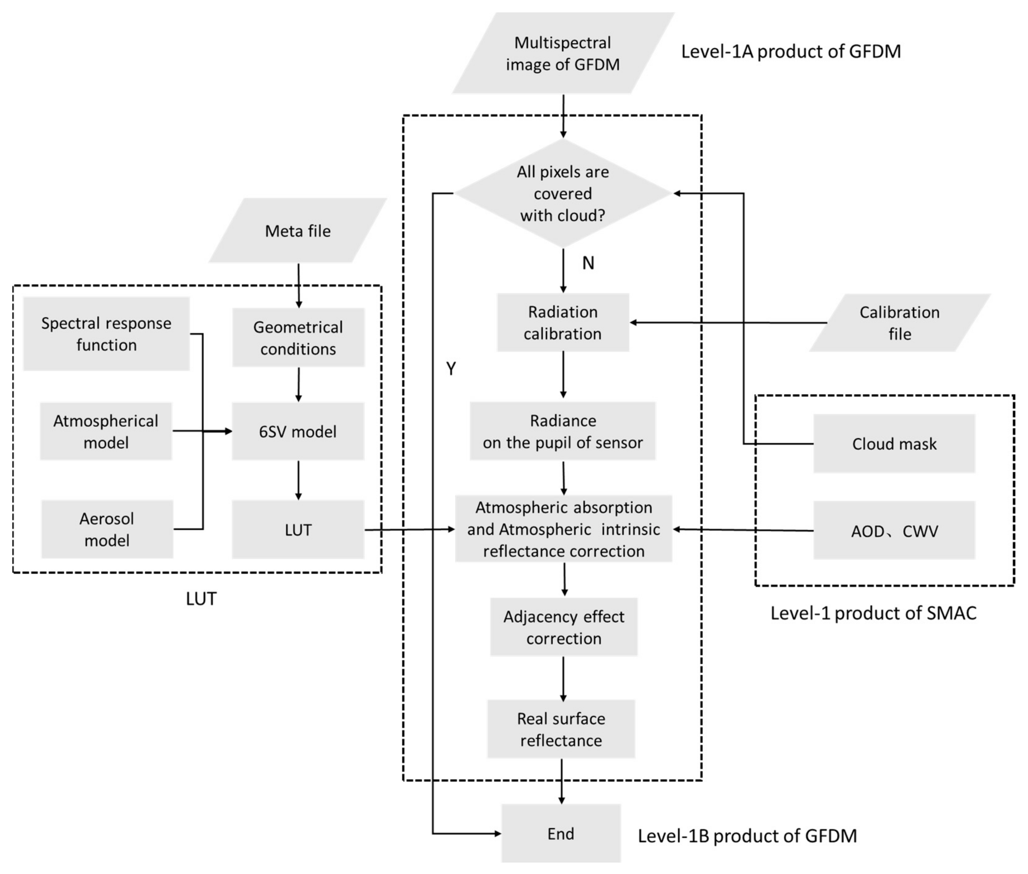
3.3. Synchronization Atmospheric Correction

Considering atmospheric scattering, together with the radiance directly reflected off the corresponding ground surface along the ground-to-sensor direction, a single sensor pixel collects two different contributions [37,38,39]: radiation diffused by the atmosphere without interaction with the ground (called path radiance); then, radiance scattered by the neighbor pixels through scattering events (called adjacency effect). The main contributions are depicted in Figure 4. Atmospheric correction mainly removes the influence of atmospheric and adjacency effects for retrieving the real reflectance of ground objects [4]. The principles of atmospheric correction follow those reported in a study by Tang et al. [40].

First, radiometric calibration is performed on each pixel to transform the DN value into the spectral radiance as

$$L=C_0\cdot DN+C_1,$$

(16)

where $C_0$ denotes the gain coefficient, and its unit is equal to ${\mathrm{W}\mathrm{m}}^{-2}{\mathrm{sr}}^{-1}{\mathsf{\mu }\mathrm{m}}^{-1}$, and $C_1$ represents the offset. $C_0$ and $C_1$ are obtained from the calibration file provided by the CNSA.

Additionally, the spectral radiance $L$ can be expressed as

$$L=L_{path}+T({\theta }_v)\frac{{\rho }_1{E}_g(0)}{\pi (1-{\rho }_{1}S)},$$

(17)

where $L_{path}$ denotes the path radiance. ${\theta }_v$ symbolizes the viewing zenith angle. ${\rho }_1$ denotes the surface reflectance, which includes the interference of the adjacency effect.$T({\theta }_v)$ represents the atmospheric transmittance in total along the ground-to-sensor direction; $E_g(0)$ represents the solar irradiance corresponding to the position; and $S$ denotes the atmospheric hemispheric albedo. For this step, the image parameters are used as inputs for 6SV model [39]. Thereafter, considering all of the reasonably likely atmospheric conditions, a LUT is established, containing $L_{path}$ and $T({\theta }_v)$, etc.

Subsequently, the initial surface reflectance ${\rho }_1$ can be calculated as

$${\rho }_1=\frac{L-L_{path}}{\frac{T({\theta }_{\mathrm{v}})E_g}{\pi }+(L-L_{path})S},$$

(18)

Accordingly, the contribution ${\rho }_M$ of the surrounding pixels can be calculated as [40]

$${\rho }_M={\displaystyle \sum _k{\displaystyle \sum _l{\rho }^{\prime }}}(x,y)P(x,y,{\theta }_v),$$

(19)

where ${\rho }^{\prime }(x,y)$ is the reflectance of the neighboring pixel in row $x$ and column $y$, and $P(x,y,{\theta }_v)$ is a weight function describing the contribution rate of the neighboring pixel, which depends on the distance, $r$, from the target pixel. The weight factor changes dynamically according to the spatial distance from the central pixel to its neighboring pixels and the reflectance difference between the central pixel and its neighboring pixels [4].

Finally, adjacency effect correction is performed, and the surface reflectance ${\rho }_t$ can be obtained as [40]

$${\rho }_t={\rho }_1+q({\rho }_1-{\rho }_M),$$

(20)

where $q$ represents the coefficient of the adjacency effect correction, and it equals to the ratio of the background radiance and the pixel radiance [41]. The principles of synchronization atmospheric correction based on the SMAC are illustrated in Figure 5.

4. Experiments

4.1. Data Sets

• Satellite data

The GFDM satellite provides high-resolution satellite images with a 0.42 m panchromatic resolution and a 1.6 m multispectral resolution. In the experiments, six multispectral images under various atmospheric conditions were chosen to apply atmospheric correction. The scenes are centered on three radiometric calibration sites located in Dunhang, Songshan, and Baotou, respectively. Furthermore, field-based test measurements were conducted on the sites, and the collected data could be used for performance tests of Syn-AC.

Table 4. Atmospheric parameters and observed geometric conditions of the images of Dunhuang, Songshan, and Baotou.

	Location	Imaging Time (UTC)	Image Center	Satellite Zenith	Satellite Azimuth	Aerosol Model
Example 1	Dunhuang	2020/7/27 4:34:17	40.092°N, 94.404°E	4.319°	90.854°	Continental
Example 2	Songshan	2020/8/26 3:24:14	34.514°N, 113.103°E	31.087°	217.135°	Continental
Example 3		2021/2/4 3:40:24	34.553°N, 113.109°E	36.934°	283.133°	Continental
Example 4		2021/2/8 3:37:06	34.554°N, 113.1°E	31.696°	286.942°	Continental
Example 5	Baotou	2020/8/26 3:21:55	40.843°N, 109.636°E	28.782°	96.381°	Continental
Example 6		2020/8/31 3:42:14	40.895°N, 109.65°E	10.389°	285.117°	Continental

lists the corresponding geometric observation conditions of the images, and the imaging time means the start time and date of main sensor shooting on the ground targets. Based on the previous experience and data analyses, the “Continental” aerosol model tends to perform better in the selected cases.

• Study area

As shown in Figure 6, the fields marked with red square are study areas, where field-based test measurements were conducted. In the Dunhuang site, the Gobi surface (Figure 6a) commonly used in radiometric calibration was selected as the experimental target in this study [13]. Additionally, the black target with 5% reflectivity and the white target with 60% reflectivity [14] in the Songshan site (Figure 6b) were chosen as experimental targets. In the Baotou calibration site shown in Figure 6c, three targets with different reflectivity [15] were selected as experimental targets.

In the field-based test measurements, a spectroradiometer produced by Analytical Spectral Devices (ASD) was used to collect spectral data on the target surface. The spectroradiometer collected wavelengths in a spectral range from 400 to 1600 nm with 1 nm sampling interval. Following the spectral measurement specification [42], the measurements were conducted under cloudless atmosphere condition. For each target, three repeated observations perpendicular to the target surface were taken, and the average value was taken as the target spectrum.

In order to compare the reflectance retrievals of AC with the field-measured values, the normalized average reflectance corresponding to each band of the GFDM satellite was obtained using Equation (21) as [43]

$${\rho }_{average}=\frac{{\displaystyle {\int }_{{\lambda }_1}^{{\lambda }_2}L(\lambda ){\rho }_{field}(\lambda )d\lambda }}{{\displaystyle {\int }_{{\lambda }_1}^{{\lambda }_2}L(\lambda )d\lambda }},$$

(21)

where ${\rho }_{field}$ denotes the average reflectance spectrum and $L$ represents the relative spectral radiance response of the GFDM multispectral band; ${\lambda }_1=400 \mathrm{nm}$, and ${\lambda }_2=1040\mathrm{nm}$. As shown in

Table 5. Detailed information of field-based test measurements.

Location		Dunhuang	Songshan		Baotou
Time (UTC)		2020/7/27 12:34	2020/8/26 3:24		2020/9/10 3:19
Targets		Sand	White	Black	White	Gray	Black
Average reflectance	485 nm	0.173	0.432	0.040	0.429	0.116	0.059
	555 nm	0.211	0.484	0.040	0.464	0.147	0.068
	607.5 nm	0.232	0.508	0.040	0.478	0.159	0.071
	660 nm	0.237	0.512	0.040	0.482	0.161	0.073
	725 nm	0.240	0.516	0.040	0.493	0.166	0.076
	830 nm	0.240	0.507	0.041	0.498	0.171	0.072
	950 nm	0.236	0.477	0.038	0.497	0.172	0.066
Max standard deviation of field-based measurement		0.0089	0.0110	0.0018	0.0046	0.0018	0.0004

, the detailed information of the field-based test measurements is listed. The maximum standard deviation of the measurements for six targets were 0.0089, 0.01109, 0.00180, 0.00462, 0.0018, and 0.00039, respectively. It can be seen that the target spectra from the Dunhuang and Songshan sites were synchronously measured as the GFDM satellite passed over on 27 July 2020 and 26 August 2020, respectively. Therefore, it is assumed that the spectral reflectance of the target surface within a short time changes insignificantly, and the artificial target has a uniform Lambert surface [44], so the field measured data could be used for experimental analyses.

• AOD (550 nm) and CWV

The accuracy of atmospheric parameters has a great influence on the accuracy of AC, therefore, it is necessary to analyze the accuracy of the retrieved AOD and CWV before applying Syn-AC. In this study, the products from ground-based sites were used for a comparative analysis of the selected cases. In terms of temporal matching, the average value of at least two ground-based observations within 30 min before and after the satellite passed over is used [45]. For the Dunhuang case, the atmospheric parameters measured by the CNSA during on-orbit calibration on 27 July 2020 were used. The data in

Table 6. Ground-based sites and observations.

	Imaging Time (UTC)	Data Source	Site		Observation Time 1 (UTC)	Observation Time 2 (UTC)
			Longitude	Latitude
Example 1	2020/7/27 4:34:17	CNSA	94.404°E	40.092°N	2020/7/27 4:34:17	-
Example 2	2020/8/26 3:24:14	SONET	113.114°E	34.511°N	2020/8/2 3:15:27	2020/8/26 3:30:28
Example 3	2021/2/4 3:40:24				-	2021/2/4 4:08:58
Example 4	2021/2/8 3:37:06				2021/2/8 3:28:00	2021/2/8 3:42:55
Example 5	2020/8/26 3:21:55	AERONET	109.629°E	40.852°N	2020/8/26 3:14:19	2020/8/26 3:29:26
Example 6	2020/8/31 3:42:14				2020/8/31 3:27:51	2020/8/31 3:42:52

are detailed information of the ground-based sites and the corresponding ground observations used in the experiment’s analysis.

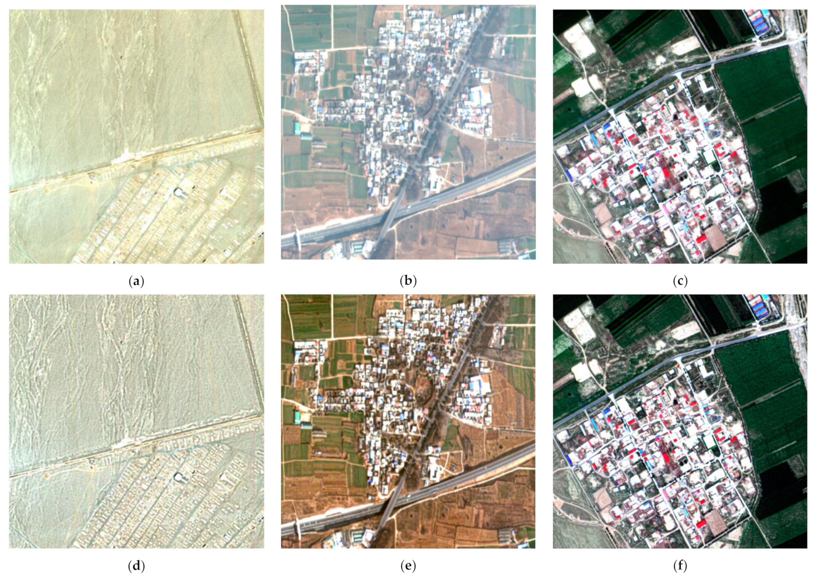
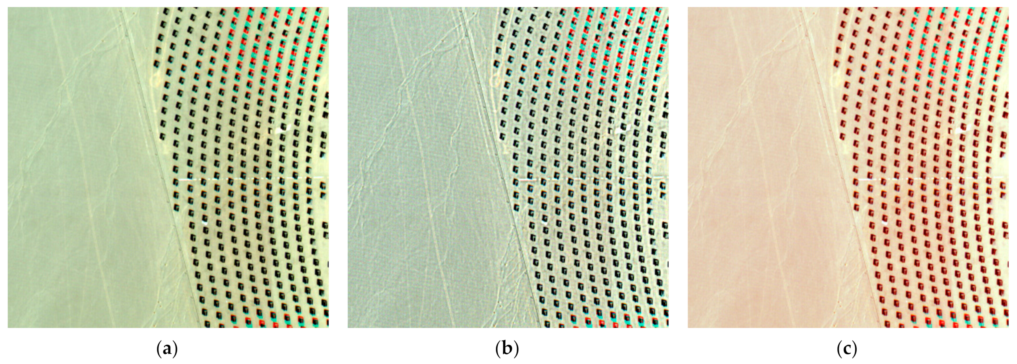
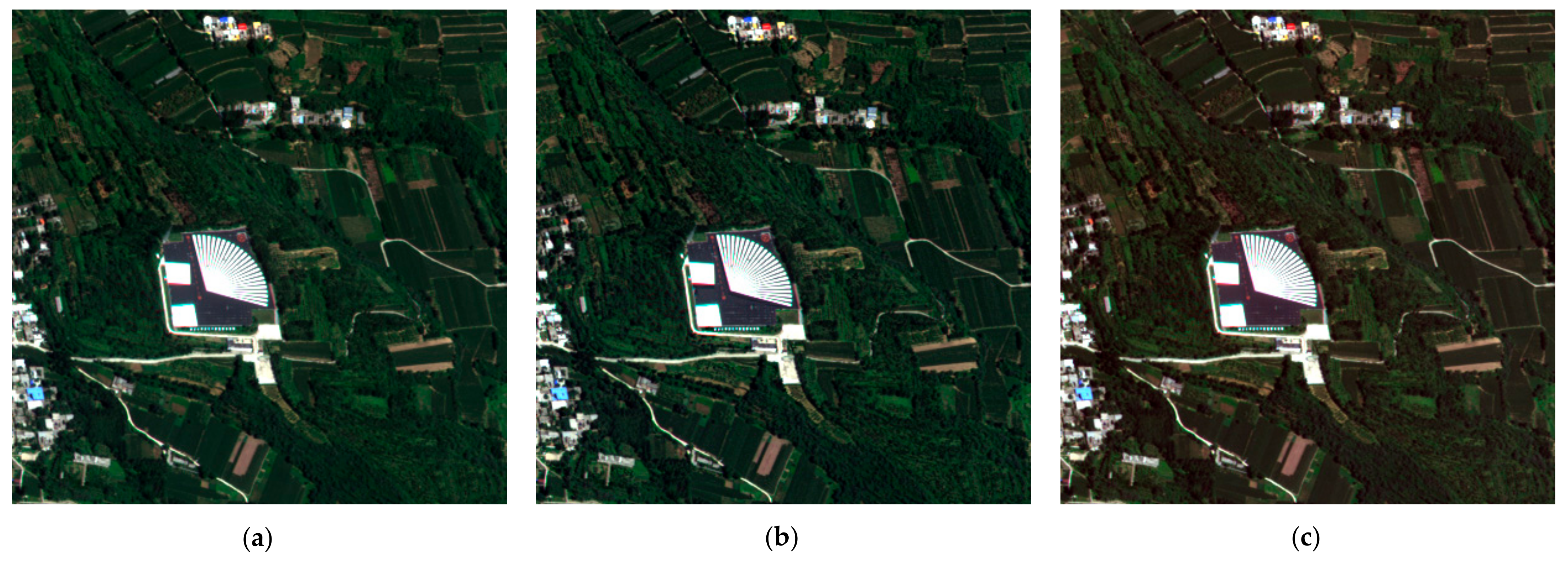
4.2. Comparison of Visual Effects before and after AC

The scattering of solar radiation by the atmospheric molecules and aerosol tend to cause the blurring of satellite images [46]. Atmospheric correction can effectively remove the influence of the atmosphere, and the blurring effect of the atmosphere is reduced after atmospheric correction. In particular, if the adjacency effect is corrected, better clarity and contrast are achieved [47]. Therefore, the visual effects of the satellite images before and after atmospheric correction were compared in the study.

4.3. Correction Precision

As described in Section 3, the output of Syn-AC is the surface reflectance after removing atmospheric influence and the interference contribution of the surrounding pixels. The accuracy of the reflectance retrievals is critical for remote sensing quantitative application. To validate the correction precision of Syn-AC, the average reflectance of the selected targets in the surface reflectance image of Syn-AC was compared with the field-measured value, and the absolute error (E_A) and the relative error (E_R, %) between reflectance retrievals and field measurements was calculated for each band following Equations (22) and (23), respectively.

$$E_{\mathrm{A}}=|{\rho }_t-{\rho }_{field}^{}|,$$

(22)

$$E_{\mathrm{R}}=|{\rho }_t-{\rho }_{field}^{}|/{\rho }_{field},$$

(23)

where ${\rho }_t$ denotes the reflectance retrieval and ${\rho }_{field}$ denotes the field-measured value.

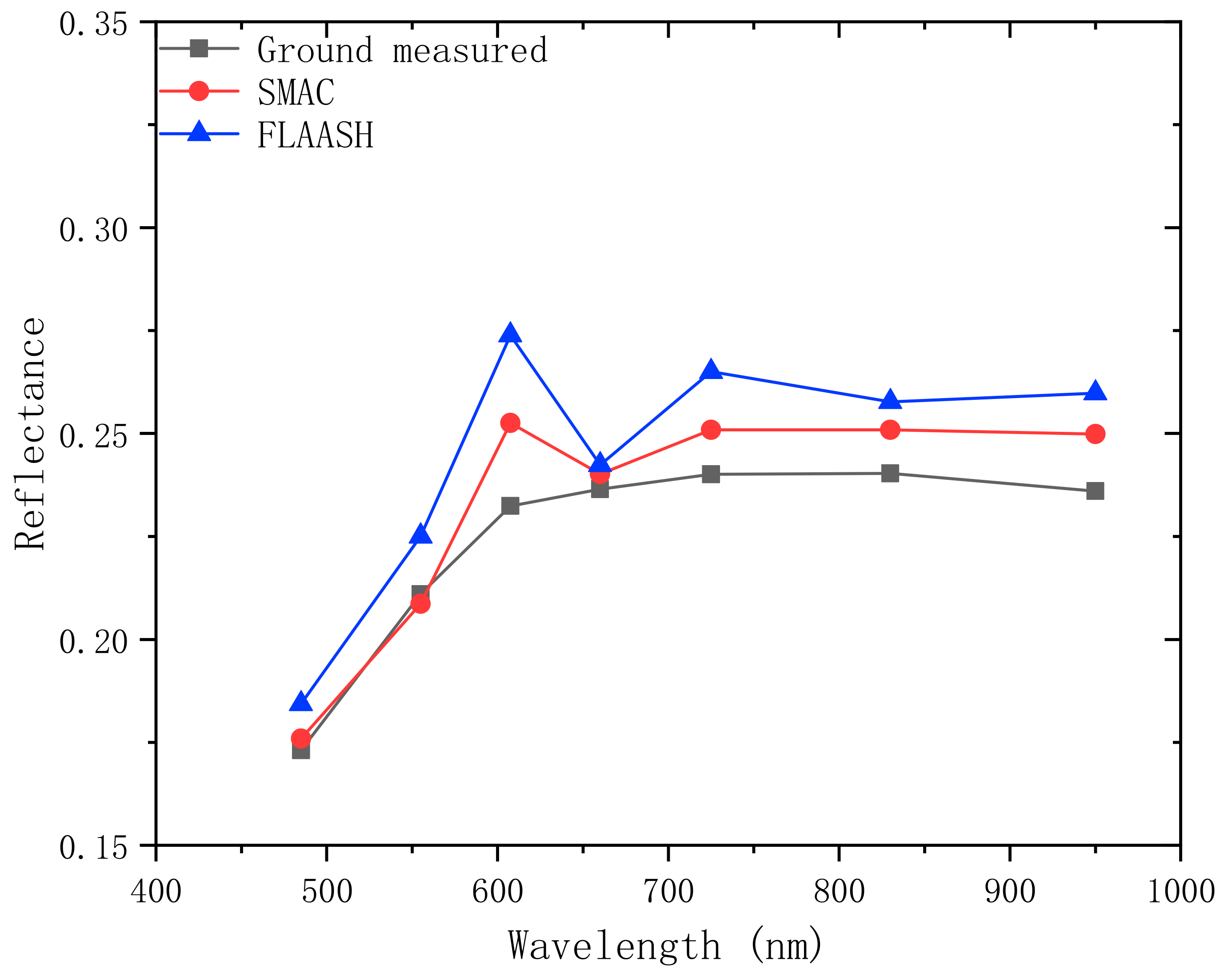
4.4. Comparison with FLAASH

The fast line-of-sight atmospheric analysis of spectral hypercubes (FLAASH), a classical atmospheric correction model, was introduced into the experiments [48]. Then, the validation of the correction precision of FLAASH was conducted in the same way as for Syn-AC. FLAASH is based on the radiative transfer model code, MODTRAN 4.0, which is written in FORTRAN [48]. The model is the first principle atmospheric correction model that can correct wavelengths from visible and near-infrared (VNIR), short-wave infrared (SWIR), and 3000 nm spectral range [49]. Moreover, the FLAASH model considers the adjacency effect, and the input data must be the calibrated image. Moreover, the imaging parameters were inputted according to the metadata of the image. The atmospheric model was calculated according to the flight date and scene center location [49]. The aerosol model was the same as the input of Syn-AC. Independent of the synchronously measured atmospheric parameters, FLAASH can estimate atmospheric properties on the basis of spectral information from each pixel of the image to be corrected [48]. Meanwhile, the correction precision between Syn-AC and FLAASH was compared.

5. Results

5.1. Atmospheric Retrieval Results of SMAC

A preliminary validation of the atmospheric parameters retrieved from the SMAC against AERONET was performed, with the results indicating that the synchronized atmospheric parameters retrieved from the SMAC are consistent with the ground measurements [16]. The data in

Table 7. Comparison between AOD (550 nm) and CWV (g/cm²) retrieved from SMAC and the ground-based observation.

	Site	Date	AOD (550 nm)			CWV (g/cm2)
			Ground Measured	SMAC	ER (%)	Ground Measured	SMAC	ER (%)
Example 1	Dunhuang	27 July 2020	0.164	0.200	22	1.808	1.67	8
Example 2	Songshan	26 August 2020	0.200	0.225	13	2.506	2.42	3
Example 3		4 February 2021	0.417	0.421	1	0.486	0.42	14
Example 4		8 February 2021	1.061	1.19	12	0.871	0.72	17
Example 5	AOE_Baotou	26 February 2020	0.314	0.338	8	1.455	1.42	2
Example 6		31 February 2020	0.081	0.092	14	1.179	1.14	3

are the atmospheric parameters retrieved from the SMAC corresponding to the selected examples contrasting with those obtained from the ground-based sites, and the relative error (E_R, %) were calculated. The results indicate that the synchronized atmospheric parameters retrieved from SMAC have good agreement with the ground measurements, and the atmospheric retrievals could be used for atmospheric correction in Syn-AC.

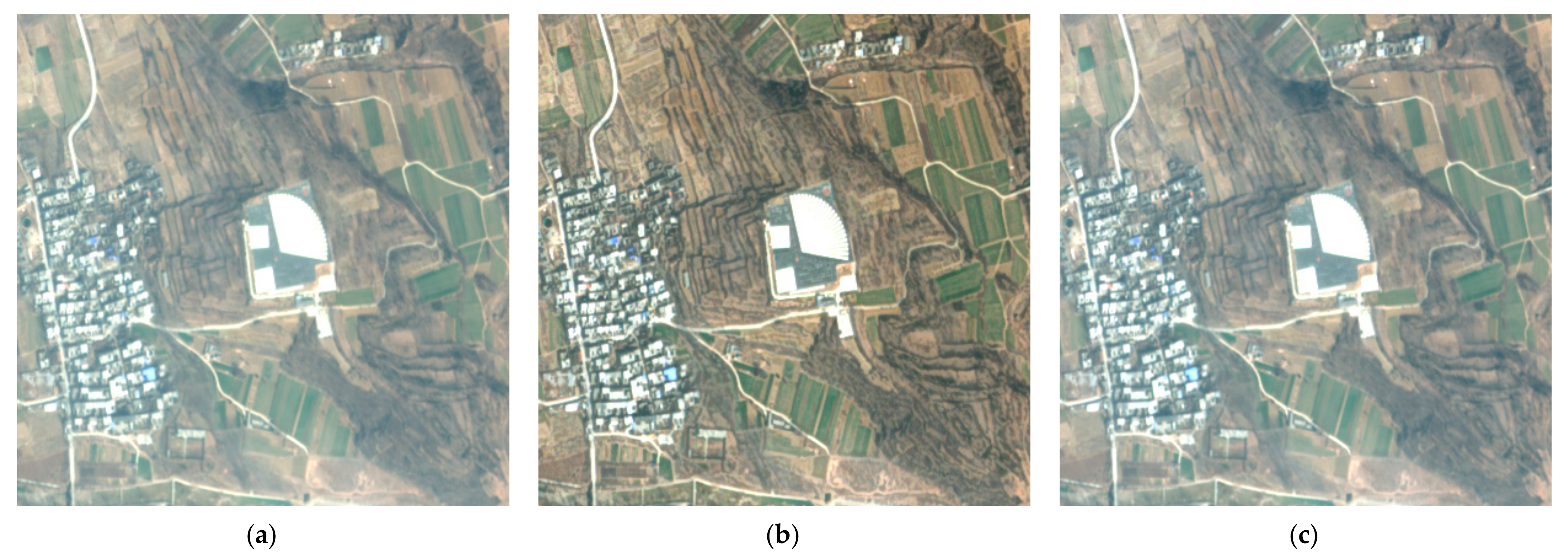
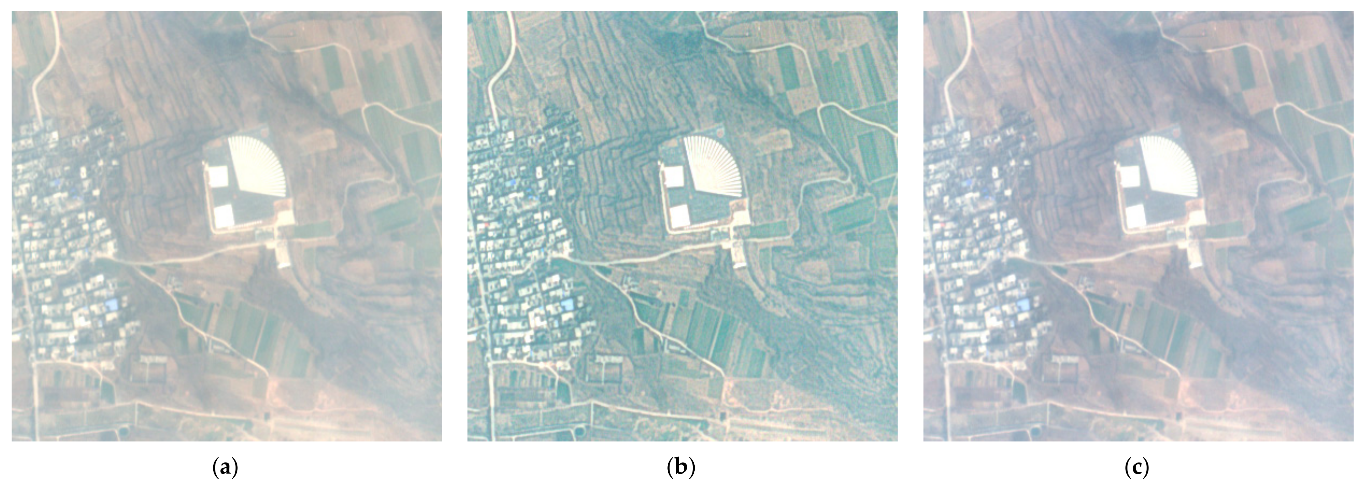
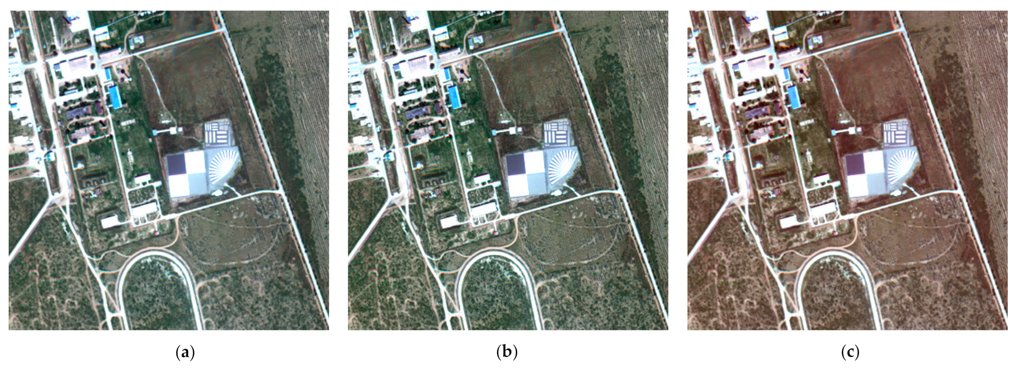
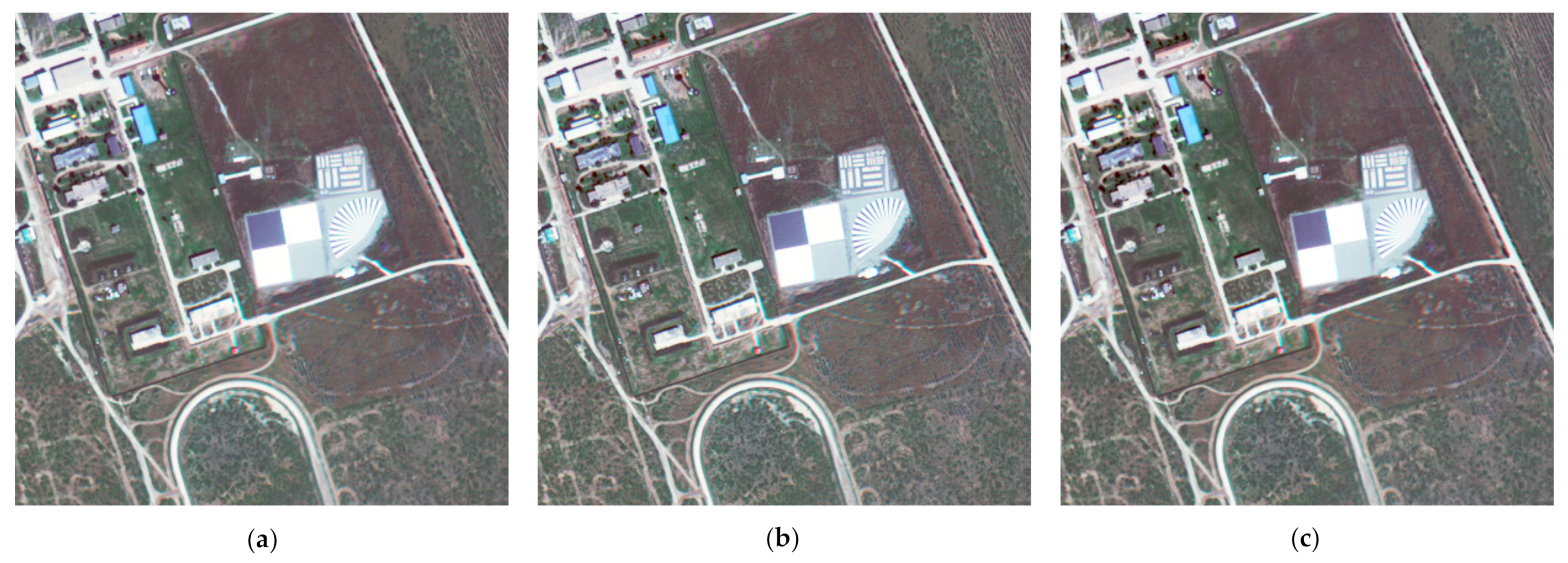
5.2. Comparison of Visual Effects before and after AC

Based on the synchronous AOD and CWV retrieved from the SMAC, synchronization atmospheric correction was applied to each image of the datasets. For the sake of simplicity, three images under different atmospheric conditions were selected, and parts of the images before and after Syn-AC are depicted in Figure 7. The AC parameters retrieved from SMAC data are the AOD of 0.2, 0.421, and 0.092, and the CWV of 1.67, 0.42, and 1.14 g/cm² for images (a)–(c), respectively. In the upper panel, Figure 7a–c present the true color images (formed by band 3, 2, and 1 for red, green, and blue, respectively) before AC, which are blurred. In contrast, the true color images after AC exhibit clear image edges and rich textures, as shown in the bottom panel.

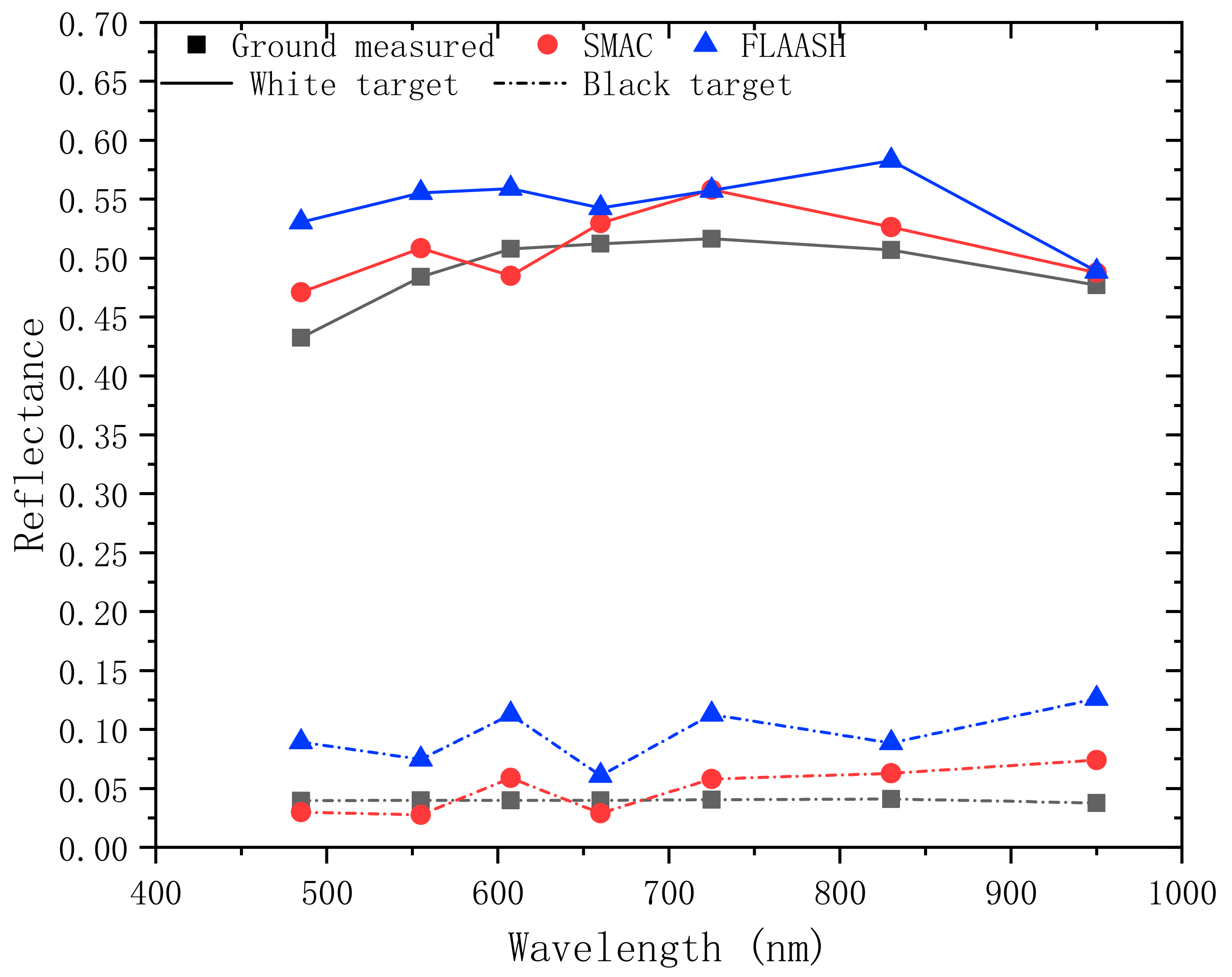
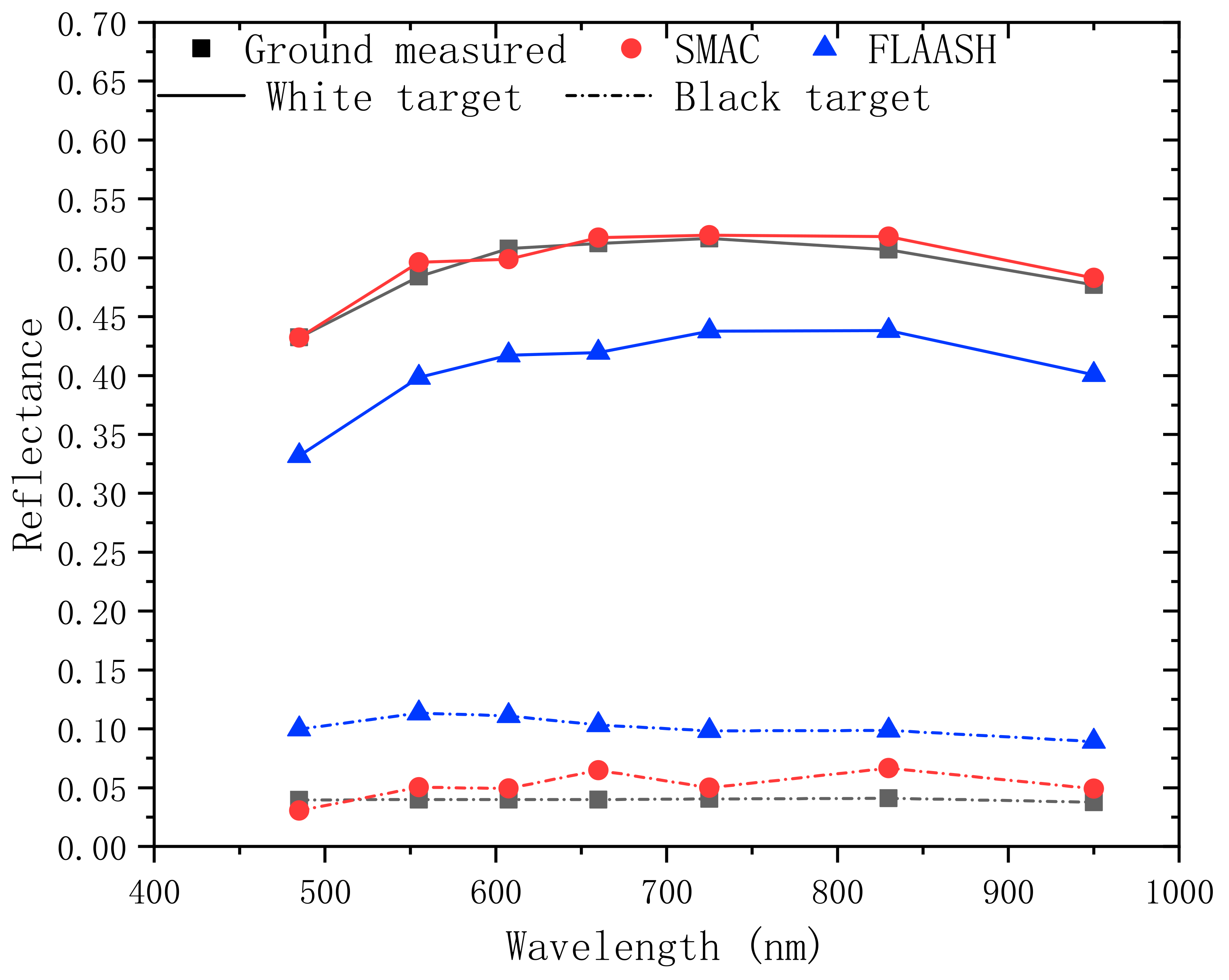
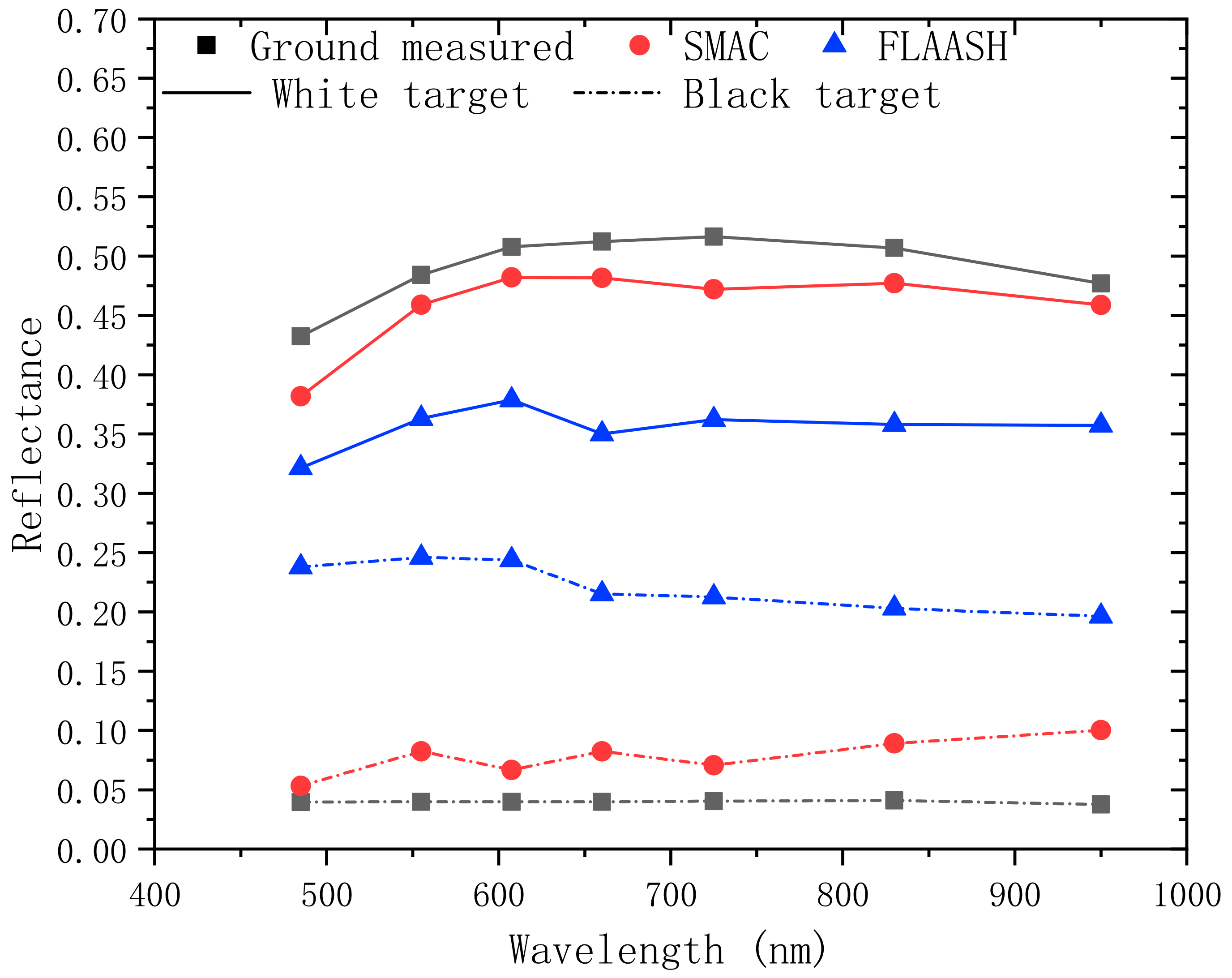
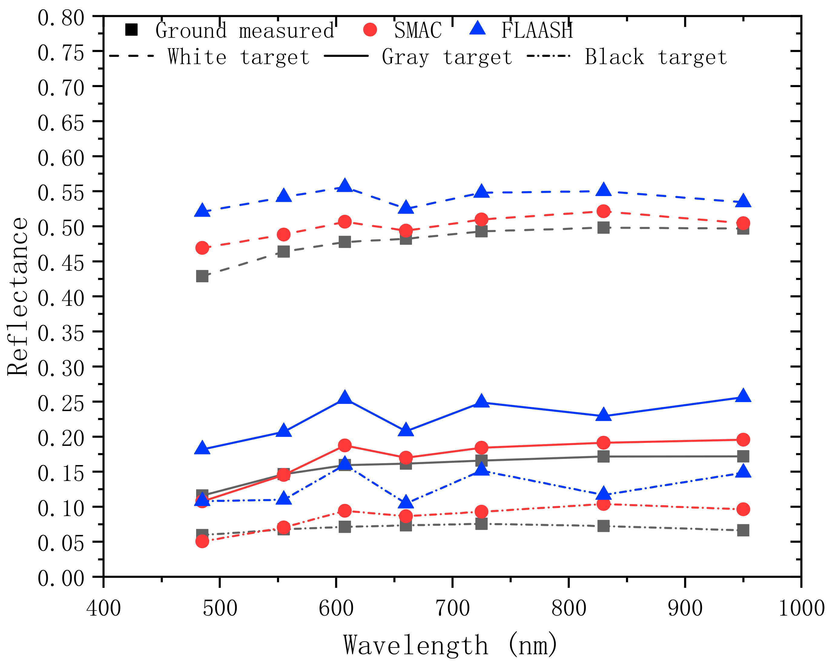
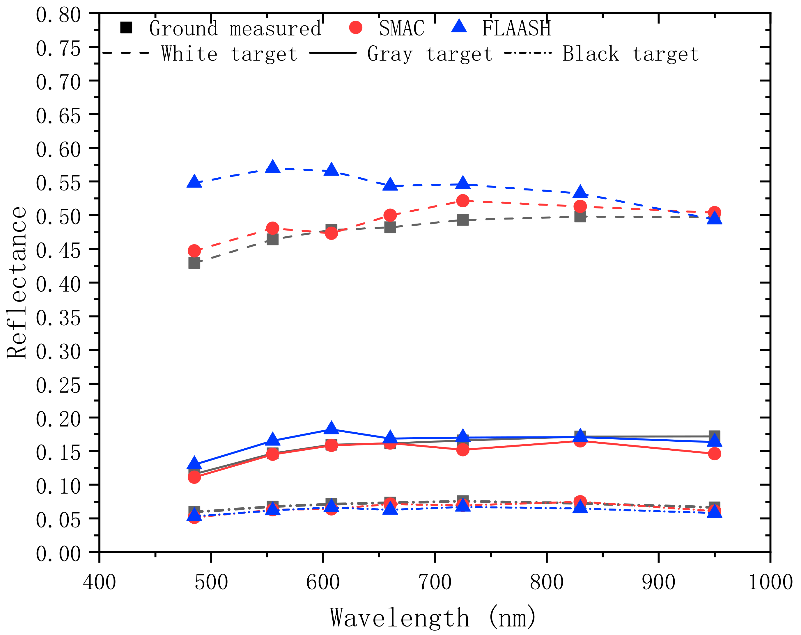
5.3. Correction Precision

An image composed of reflectance retrievals was generated after atmospheric correction. In this part, the images of the study area in the original and corrected images are displayed. Then, the average reflectance of the targets in the surface reflectance image obtained after atmospheric correction was calculated and compared with the field-based measurement value to verify the accuracy of AC in quantitative applications. In order to compare the correction accuracy, the reflectance retrievals of Syn-AC and FLAASH are listed, and the absolute error (E_A) and the relative error (E_R, %) between the reflectance retrievals and field-based measurement values were calculated.

• Dunhuang

The Syn-AC and FLAASH methods were applied to perform AC on the GFDM multispectral image of Dunhuang (Figure 8a). The average surface reflectance in the study region of each image of Figure 8b,c was analyzed, and the results are illustrated in Figure 9. As indicated in Figure 9, the values obtained from the surface reflectance images of the Syn-AC and FLAASH methods are in good agreement with the field-measured data. As indicated in

Table 8. Performance comparison for sand between Syn-AC and FLAASH, based on Example 1.

Site	Songshan—Example 1
Target	Sand
	Syn-AC		FLAASH
Band/nm	EA	ER (%)	EA	ER (%)
485	0.0028	1.6	0.0112	6.5
555	0.0024	1.1	0.0141	6.7
607.5	0.0201	8.7	0.0415	17.9
660	0.0037	1.6	0.0059	2.5
725	0.0108	4.5	0.0249	10.4
830	0.0106	4.4	0.0174	7.2
950	0.0139	5.9	0.0238	10.1

, the E_R values between the reflectance retrievals from Syn-AC and the ground-measured value are smaller. The absolute error values of Syn-AC are within 0.0201, and the max absolute error of FLAASH is 0.0415. The mean relative error values of Syn-AC and FLAASH are 4.0% and 8.7%, respectively.

• Songshan

For the artificial target site located in Songshan, three multispectral images under different atmospheric conditions were selected for quantitative research. Syn-AC and FLAASH were applied to perform AC on these images. The atmospheric correction parameter retrievals are obtained from the SMAC with AOD of 0.225, 0.421, and 1.19, as well as CWV of 2.42, 0.42, and 0.72 g/cm² for Figure 10a, Figure 12a and Figure 14a, respectively.

For the case of the slightly polluted atmosphere (Figure 10a), the surface reflectance images after AC are shown in Figure 10b,c. As shown in Figure 11, the overall results of Syn-AC of the white target are proximate to the measured values. As shown in

Table 9. Performance comparison between Syn-AC and FLAASH, basing on Example 2.

Site	Songshan—Example 2
Target	White Target				Black Target
	Syn-AC		FLAASH		Syn-AC		FLAASH
Band/nm	EA	ER (%)	EA	ER (%)	EA	ER (%)	EA	ER (%)
485	0.0386	8.9	0.0981	22.7	0.0098	24.7	0.0496	124.9
555	0.0241	5.0	0.0712	14.7	0.0123	30.9	0.0349	87.8
607.5	0.023	4.5	0.051	10.0	0.019	47.7	0.0729	183.0
660	0.0176	3.4	0.0303	5.9	0.0109	27.3	0.0209	52.4
725	0.0416	8.1	0.0411	8.0	0.0176	43.5	0.0723	178.7
830	0.0194	3.8	0.0759	15.0	0.0219	53.5	0.0476	116.3
950	0.0107	2.2	0.0117	2.5	0.0364	96.5	0.0884	234.4

, the relative errors between the surface reflectance of the black target of Syn-AC and the ground measurements are smaller than that of FLAASH. For the white target, the absolute error values of Syn-AC are within 0.0416, and the max absolute error of FLAASH is 0.0981. The mean relative error values of Syn-AC and FLAASH were 5.14% and 11.25%, respectively. For the black target, the absolute error values of Syn-AC are within 0.0364, and the max absolute error of FLAASH is 0.0884. The mean relative error values of Syn-AC and FLAASH are 46.3% and 139.6%, respectively.

As for the case of the moderately polluted atmosphere, the second case of Songshan on 4 February 2021 was analyzed. The original image and the corrected images with thin cloud effectively removed are depicted in Figure 12. The contrastive results are displayed in Figure 13 and

Table 10. Performance comparison between Syn-AC and FLAASH, basing on Example 3.

Site	Songshan—Example 3
Target	White Target				Black Target
	Syn-AC		FLAASH		Syn-AC		FLAASH
Band/nm	EA	ER (%)	EA	ER (%)	EA	ER (%)	EA	ER (%)
485	0.0002	0.1	0.1007	23.3	0.0092	23.2	0.0599	150.9
555	0.012	2.5	0.0858	17.7	0.0106	26.7	0.0736	185.1
607.5	0.0091	1.8	0.0905	17.8	0.0096	24.1	0.071	178.2
660	0.005	1.0	0.0927	18.1	0.0249	62.5	0.0633	158.7
725	0.0028	0.5	0.0785	15.2	0.0095	23.5	0.0577	142.6
830	0.0111	2.2	0.0688	13.6	0.0257	62.8	0.0577	141.0
950	0.006	1.3	0.0762	16.0	0.0114	30.2	0.0513	136.0

, and the values of Syn-AC are almost identical to the field-measured values. The results of FLAASH are significantly less than the field-measured values. There is some difference between the reflectance retrievals of the black target of Syn-AC and the measured values, but the relative error is smaller than the relative error between FLAASH and the measured value. For the white target, the absolute error values of Syn-AC are within 0.012, and the max absolute error of FLAASH is 0.0927. The mean relative error values of Syn-AC and FLAASH are 1.3% and 17.4%, respectively. For the black target, the absolute error values of Syn-AC are within 0.0257, and the max absolute error of FLAASH is 0.0736. The mean relative error values of Syn-AC and FLAASH are 36.1% and 156.1%, respectively.

Considering the case of the heavily polluted atmosphere, the surface reflectance images of Syn-AC and FLAASH are shown in Figure 14b,c. The contrastive results are illustrated in Figure 15. The results of the two models are all less than the measured values, and the relative errors of Syn-AC are smaller than those of FLAASH. As shown in

Table 11. Performance comparison between Syn-AC and FLAASH, based on Example 4.

Site	Songshan—Example 4
Target	White Target				Black Target
	Syn-AC		FLAASH		Syn-AC		FLAASH
Band/nm	EA	ER (%)	EA	ER (%)	EA	ER (%)	EA	ER (%)
485	0.0505	11.7	0.111	25.7	0.0137	34.5	0.1982	499.2
555	0.0253	5.2	0.1211	25.0	0.0427	107.4	0.2063	518.7
607.5	0.0258	5.1	0.1292	25.4	0.0269	67.5	0.204	512.1
660	0.0305	5.9	0.1621	31.7	0.0425	106.6	0.1752	439.3
725	0.0442	8.6	0.1543	29.9	0.0303	74.9	0.1721	425.4
830	0.0297	5.9	0.149	29.4	0.0481	117.6	0.162	395.9
950	0.0181	3.8	0.1195	25.1	0.0625	165.7	0.1586	420.5

, the correction accuracy of the band centered on 950 nm of Syn-AC is not as good as that of other bands. The surface reflectance of black target of FLAASH is significantly different from the ground measurements. For the white target, the absolute error values of Syn-AC are within 0.0505, and the max absolute error of FLAASH is 0.1621. The mean relative error values of Syn-AC and FLAASH are 6.6% and 27.4%, respectively. For the black target, the absolute error values of Syn-AC are within 0.0625, and the max absolute error of FLAASH is 0.2063. The mean relative error values of Syn-AC and FLAASH are 96.3% and 458.7%, respectively.

• Baotou

For Baotou, two multispectral images under different atmospheric conditions were selected for a comparative analysis of Syn-AC and FLAASH. The atmospheric correction parameter retrievals are obtained from the SMAC with AOD of 0.338 and 0.092, and CWV of 1.42 and 1.14 g/cm² for Figure 16a and Figure 17a, respectively.

For the first case on 26 August 2020, the average surface reflectance in the white, gray, and black targets of each image illustrated in Figure 16 was analyzed. The reflectance retrievals and the contrastive results of white, gray, and black target are depicted in Figure 18 and

Table 12. Performance comparison between Syn-AC and FLAASH, based on Example 5.

Site	Baotou—Example 5
Target	White Target				Gray Target				Black Target
	Syn-AC		FLAASH		Syn-AC		FLAASH		Syn-AC		FLAASH
Band/nm	EA	ER (%)	EA	ER (%)	EA	ER (%)	EA	ER (%)	EA	ER (%)	EA	ER (%)
485	0.0403	9.4	0.0919	21.4	0.0084	7.2	0.0659	56.8	0.009	15.1	0.0485	81.6
555	0.024	5.2	0.0777	16.8	0.0012	0.8	0.0602	41.1	0.0027	4.0	0.0424	62.6
607.5	0.0286	6.0	0.0783	16.4	0.0282	17.7	0.0944	59.3	0.0229	32.1	0.0886	124.2
660	0.0115	2.4	0.0427	8.9	0.0083	5.1	0.0462	28.6	0.0132	18.0	0.0313	42.7
725	0.0169	3.4	0.055	11.2	0.0184	11.1	0.083	50.1	0.0174	23.1	0.0759	100.5
830	0.0232	4.7	0.0519	10.4	0.0197	11.5	0.0578	33.7	0.0315	43.5	0.0445	61.5
950	0.0078	1.6	0.0378	7.6	0.0237	13.8	0.0846	49.3	0.0299	45.0	0.0821	123.7

. The retrieved reflectance of white, gray, and black targets of Syn-AC are in good agreement with the field-measured values. Notably, the FLAASH reflectance is higher than the measured reflectance. The absolute error values of three targets (white, gray, and black) of Syn-AC are within 0.0403, 0.0282, and 0.0315, respectively. The max absolute error values of FLAASH are 0.0919, 0.0237, and 0.0886, respectively. For the white target, the mean relative error values of Syn-AC and FLAASH are 4.7% and 13.2%, respectively. For the gray target, the mean relative error values of Syn-AC and FLAASH are 9.6% and 45.6%, respectively. For the black target, the mean relative error values of Syn-AC and FLAASH are 25.8% and 85.2%, respectively.

For the image on 31 August 2020, the AOD retrieved from SMAC was 0.092. As depicted in Figure 17, the atmospheric condition is clear. As shown in Figure 19 and

Table 13. Performance comparison between Syn-AC and FLAASH, based on Example 6.

Site	Baotou—Example 6
Target	White Target				Gray Target				Black Target
	Syn-AC		FLAASH		Syn-AC		FLAASH		Syn-AC		FLAASH
Band/nm	EA	ER (%)	EA	ER (%)	EA	ER (%)	EA	ER (%)	EA	ER (%)	EA	ER (%)
485	0.0183	4.3	0.119	27.8	0.0048	4.1	0.0139	12.0	0.0077	13.0	0.0062	10.4
555	0.0166	3.6	0.1056	22.8	0.0014	1.0	0.0187	12.8	0.0052	7.7	0.0061	9.0
607.5	0.0046	1.0	0.0877	18.4	0.0009	0.6	0.0226	14.2	0.0072	10.1	0.005	7.0
660	0.0176	3.7	0.0613	12.7	0.0004	0.3	0.0071	4.4	0.0021	2.9	0.0106	14.5
725	0.0285	5.8	0.0529	10.7	0.0137	8.3	0.0044	2.7	0.006	8.0	0.0082	10.0
830	0.0149	3.0	0.0341	6.9	0.0064	3.7	0.0008	0.5	0.0023	3.2	0.0077	10.6
950	0.0072	1.5	0.003	0.6	0.0258	15.0	0.0083	4.8	0.0056	8.4	0.0084	12.7

, the average reflectance of white, gray, and black targets obtained from the surface reflectance image of Syn-AC are identical to the field-measured values. The correction precision of FLAASH is inferior to that of Syn-AC. The absolute error values of three targets (white, gray, and black) of Syn-AC are within 0.0285, 0.0258, and 0.0077, respectively. The max absolute error values of three targets of FLAASH are 0.119, 0.0226, and 0.0106, respectively. For the white target, the mean relative error values of Syn-AC and FLAASH are 3.2% and 14.3%, respectively. For the gray target, the mean relative error values of Syn-AC and FLAASH are 4.7% and 7.3%, respectively. For the black target, the mean relative error values of Syn-AC and FLAASH are 7.6% and 10.7%, respectively.

6. Discussion

High-precision atmospheric parameters are critical for atmospheric correction based on the radiative transfer model and quantitative application of high spatial resolution remote sensing images. However, due to the spatial-temporal variation of atmospheric parameters, the traditional method of obtaining atmospheric parameters based on ground-based sites or other satellite products is difficult to ensure the spatial and temporal matching between atmospheric parameters and images, resulting in the error of atmospheric correction. The present paper has demonstrated that the solution to obtain atmospheric parameters synchronously by the equipment on-board the satellite platform is effective.

Based on the synchronous atmospheric parameters, atmospheric correction experiments of GFDM satellite images were conducted. Compared with the original image, the visual effects of corrected image were improved with the blurring effect removed. In addition, the better clarity and contrast were achieved after adjacency effect correction. In the case of lower atmospheric visibility, the correction effect was more obvious, and the image quality was of greater improvement.

The correction precision of Syn-AC was verified by comparing with the field-measured reflectance, and the same analysis was performed for FLAASH. The two methods are both based on radiative transfer models, and other inputs including satellite imaging parameters, atmospheric model, and aerosol model are the same except for the sources of atmospheric parameters. The results indicate that both methods performed well. However, most of the reflectance retrievals error of Syn-AC were less than those of FLAASH, and the correction performance of Syn-AC was more stable. It is considered that FLAASH estimates atmospheric parameters based on the spectral information in the remote sensing image, whereas the band settings of the main sensor may not meet the requirements of FLAASH to retrieve atmospheric parameters. On the other hand, the atmospheric parameters of Syn-AC were retrieved from SMAC, which is specifically designed to detect atmospheric information. Therefore, most of the retrieved values of Syn-AC were closer to the field-measured values.

The acquisition of satellite image of study area requires the imaging schedule submitted by CNSA in advance, so the image data of the region of interest is limited. According to the current experimental results, more image data are required for the analysis of the correction performance under different atmospheric states and underlying surface, as well as the influence of atmospheric model and aerosol model on correction accuracy.

7. Conclusions

In view of the temporal and spatial variation of the atmospheric state, the atmospheric correction on remote sensing images based on synchronous atmospheric parameters could provide a higher precision. An atmospheric correction method was proposed based on the synchronization atmospheric parameters retrieved from SMAC, including the processing steps for the SMAC data, main ideas of atmospheric parameters inversion, and the principles of atmospheric correction of GFDM satellite images. Additionally, based on the atmospheric parameters retrieved from SMAC data, experiments were conducted to investigate the performance and verify the correction precision of the Syn-AC method.

In the present study, six images of three radiometric calibration sites were selected. First, the data obtained from ground-based sites were used to analyze the accuracy of the atmospheric parameters retrieved from SMAC. The max relative errors of AOD and CWV were 22% and 17%, respectively. The results show that the atmospheric parameters retrieved from SMAC in the study are in good agreement with the ground observations, and the atmospheric retrievals could be used in atmospheric correction of GFDM satellite imagery.

For the selected images, Syn-AC and FLAASH were applied to conduct correction experiments. Then, the average reflectance of the targets from the corrected image of Syn-AC and FLAASH were compared with the field-measured reflectance to test correction precision. The max absolute error of Syn-AC was 0.0625, representing a higher precision than the FLAASH (the max absolute error was 0.2063). The mean relative error of Syn-AC and FLAASH were 19.3% and 76.6%, respectively (in the view of the fact that the reflectance of the black target is close to 0, and the measured value is within 0.1. Even if the deviation between the retrieved reflectance and the measured reflectance value is small, a large relative error may be calculated).

Preliminary analyses of the performance of Syn-AC indicate that the atmospheric parameters measured synchronically are useful to improve image quality and obtain high-precision surface reflectance than those based on image spectral information inversion. The SMAC is of great potential to further meet the demand of high-precision data for remote sensing application, which indicates the necessity of synchronous atmospheric parameters.

At present, an atmospheric synchronization correction instrument capable of imaging is being developed. Therefore, it is urgent to conduct research on atmospheric correction based on image of the atmospheric corrector and spectral polarization information, and the study of this paper is an important part.

References

1. Goody, R.M.; Yung, Y.L. Atmospheric Radiation: Theoretical Basis; Oxford University Press: New York, NY, USA, 1989. [Google Scholar] [CrossRef]
2. Shettle, E.P. Models of aerosols, clouds, and precipitation for atmospheric propagation studies. In AGARD, Atmospheric Propagation in the UV, Visible, IR, and MM-Wave Region and Related Systems Aspects; The SAO/NASA Astrophysics Data System: Silicon Valley, SF, USA, 1990; 14p. [Google Scholar]
3. Guzzi, D.; Nardino, V.; Lastri, C.; Raimondi, V. A Fast Iterative Procedure for Adjacency Effects Correction on Remote Sensed Data. Remote Sens. 2021, 13, 1799. [Google Scholar] [CrossRef]
4. Wang, T.; Du, L.; Yi, W.; Hong, J.; Zhang, L.; Zheng, J.; Li, C.; Ma, X.; Zhang, D.; Fang, W.; et al. An adaptive atmospheric correction algorithm for the effective adjacency effect correction of submeter-scale spatial resolution optical satellite images: Application to a WorldView-3 panchromatic image. Remote Sens. Environ. 2021, 259, 112412. [Google Scholar] [CrossRef]
5. Li, Z.Q.; Chen, X.F.; Ma, L.Y.; Qie, L.L.; Hou, W.Z.; Qiao, Y.L. Review of atmospheric correction for optical remote sensing satellites. J. Nanjing Univ. Inf. Sci. Technol. Nat. Sci. Ed. 2018, 10, 10. [Google Scholar] [CrossRef]
6. Smirnov, A.; Holben, B.N.; Eck, T.F.; Slutsker, I.; Chatenet, B.; Pinker, R.T. Diurnal variability of aerosol optical depth observed at AERONET (Aerosol Robotic Network) sites. Geophys. Res. Lett. 2002, 29, 30-1–30-4. [Google Scholar] [CrossRef]
7. Ma, Y. Study on Synchronous Atmospheric Correction of High Spatial Resolution Optical Remote Sensing Satellite; University of Chinese Academy of Sciences: Beijing, China, 2016. [Google Scholar]
8. Kaufman, Y.J.; Sendra, C. Algorithm for automatic atmospheric corrections to visible and near-IR satellite imagery. Int. J. Remote Sens. 1988, 9, 1357–1381. [Google Scholar] [CrossRef]
9. Levy, R.C.; Mattoo, S.; Munchak, L.A.; Remer, L.A.; Sayer, A.M.; Patadia, F.; Hsu, N.C. The Collection 6 MODIS aerosol products over land and ocean. Atmos. Meas. Tech. 2013, 6, 2989–3034. [Google Scholar] [CrossRef]
10. Dubovik, O.; Schuster, G.L.; Xu, F.; Hu, Y.; Bösch, H.; Landgraf, J.; Li, Z. Grand Challenges in Satellite Remote Sensing. Front. Remote Sens. 2021, 2, 619818. [Google Scholar] [CrossRef]
11. Reuter, D.C.; McCabe, G.H.; Dimitrov, R.; Graham, S.M.; Jennings, D.E.; Matsumura, M.M.; Rapchun, D.A.; Travis, J.W. The LEISA/Atmospheric Corrector (LAC) on EO-1. In Proceedings of the IEEE International Geoscience & Remote Sensing Symposium, Sydney, NSW, Ausralia, 9–13 July 2001; IEEE: Piscataway, NJ, USA, 2001. [Google Scholar] [CrossRef]
12. Barazzetti, L.; Roncoroni, F.; Brumana, R.; Previtali, M. Georeferencing accuracy analysis of a single worldview-3 image collected over Milan. In Proceedings of the XXIII ISPRS Congress, Prague, Czech Republic, 12–19 July 2016; pp. 429–434. [Google Scholar] [CrossRef] [Green Version]
13. Fu, Q.Y.; Min, X.J.; Li, X.C.; Sha, C.; Li, X. Study on on-orbit absolute radiometric calibration of CBERS-02 CCD sensor at Dunhuang Site. Natl. Remote Sens. Bull. 2006, 10, 433–439. [Google Scholar] [CrossRef]
14. Li, Z.Z.; Xu, W.; Fu, Q.Y.; Min, X.J.; Zhang, L.M.; Pan, Z.Q.; Qiao, Y.L.; Zheng, X.B.; Fan, Y.T.; Su, B.J.; et al. Construction and application of fixed target site in Songshan Mountains, China. J. Atmos. Environ. Opt. 2014. [Google Scholar]
15. Li, C.R.; Ma, L.L.; Tang, L.L.; Gao, C.X.; Qian, Y.G.; Wang, N.; Wang, X.H. A comprehensive calibration site for high resolution remote sensors dedicated to quantitative remote sensing and its applications. Natl. Remote Sens. Bull. 2021, 25, 198–219. [Google Scholar] [CrossRef]
16. Li, Z.; Hou, W.; Qiu, Z.; Ge, B.; Xie, Y.; Hong, J.; Ma, Y.; Peng, Z.; Fang, W.; Zhang, D.; et al. Preliminary On-Orbit Performance Test of the First Polarimetric Synchronization Monitoring Atmospheric Corrector (SMAC) On-Board High-Spatial Resolution Satellite Gao Fen Duo Mo (GFDM). IEEE Trans. Geosci. Remote Sens. 2022, 60, 4104014. [Google Scholar] [CrossRef]
17. Fan, L.J.; Wang, Y.; Yang, W.T.; Yu, L.J.; Zhang, G.B. Scheme design and technical characteristics of high-resolution multimode satellite. Spacecr. Eng. 2021, 30, 10–19. [Google Scholar] [CrossRef]
18. Jiang, W.; Huang, Q.L. The high-resolution Multimode Integrated Imaging satellite was successfully launched. Spacefl. Return Remote Sens. 2020, 41, 2. [Google Scholar]
19. Hu, Y.D.; Hu, Q.Y.; Sun, B.; Wang, X.J.; Qiu, Z.W.; Hong, J. Polarization Atmospheric corrector with dual angle for remote sensing image. Opt. Precis. Eng. 2015, 023, 652–659. [Google Scholar] [CrossRef]
20. Kang, Q.; Yuan, Y.L.; Li, J.J.; Yang, W.F.; Fan, H.M.; Qian, H.H.; Wu, H.Y.; Zheng, X.B. Experimental study on filter screening method and accuracy verification of atmospheric synchronous corrector. Acta Opt. Sin. 2017, 37, s11. [Google Scholar] [CrossRef]
21. Deuzé, J.L.; Bréon, F.M.; Devaux, C.; Goloub, P.; Herman, M.; Lafrance, B.; Maignan, F.; Marchand, A.; Nadal, F.; Perry, G.; et al. Remote sensing of aerosols over land surfaces from POLDER-ADEOS-1 polarized measurements. J. Geophys. Res. Atmos. 2001, 106, 4913–4926. [Google Scholar] [CrossRef]
22. Dubovik, O.; Herman, M.; Holdak, A.; Lapyonok, T.; Tanré, D.; Deuzé, J.L.; Ducos, F.; Sinyuk, A.; Lopatin, A. Statistically optimized inversion algorithm for enhanced retrieval of aerosol properties from spectral multi-angle olarimetric satellite observations. Atmos. Meas. Tech. 2011, 4, 975–1018. [Google Scholar] [CrossRef]
23. Dubovik, O.; Li, Z.; Mishchenko, M.I.; Tanré, D.; Karol, Y.; Bojkov, B.; Cairns, B.; Diner, D.J.; Espinosa, W.R.; Goloub, P.; et al. Polarimetric remote sensing of atmospheric aerosols: Instruments, methodologies, results, and perspectives. J. Quant. Spectrosc. Radiat. Transf. 2018, 224, 474–511. [Google Scholar] [CrossRef]
24. Ge, B.; Mei, X.; Li, Z.; Hou, W.; Xie, Y.; Zhang, Y.; Xu, H.; Li, K.; Wei, Y. An improved algorithm for retrieving high resolution fine-mode aerosol based on polarized satellite data: Application and validation for POLDER-3. Remote Sens. Environ. 2020, 247, 111894. [Google Scholar] [CrossRef]
25. Levy, R.C.; Remer, L.A.; Kleidman, R.G.; Mattoo, S.; Ichoku, C.; Kahn, R.; Eck, T.F. Global evaluation of the collection 5 MODIS darktarget aerosol products over land. Atmos. Chem. Phys. 2010, 10, 10399–10420. [Google Scholar] [CrossRef]
26. Ciren, P.; Kondragunta, S. Dust aerosol index (DAI) algorithm for MODIS. J. Geophys. Res. Atmos. 2014, 119, 4770–4792. [Google Scholar] [CrossRef]
27. Hall, D.K.; Riggs, G.A.; Salomonson, V.V. Development of methods for mapping global snow cover using Moderate Resolution Imaging Spectroradiometer data. Remote Sens. Environ. 1995, 54, 127–140. [Google Scholar] [CrossRef]
28. Zheng, F.; Li, Z.; Hou, W.; Qie, L.; Zhang, C. Aerosol retrieval study from multiangle polarimetric satellite data based on optimal estimation method. J. Appl. Remote Sens. 2020, 14, 014516. [Google Scholar] [CrossRef]
29. Waquet, F.; Léon, J.F.; Cairns, B.; Goloub, P.; Deuzé, J.L.; Auriol, F.J.A.O. Analysis of the spectral and angular response of the vegetated surface polarization for the purpose of aerosol remote sensing over land. Appl. Opt. 2009, 48, 1228. [Google Scholar] [CrossRef]
30. Litvinov, P.; Hasekamp, O.; Cairns, B. Models for surface reflection of radiance and polarized radiance: Comparison with airborne multiangle photopolarimetric measurements and implications for modeling top-of-atmosphere measurements. Remote Sens. Environ. 2011, 115, 781–792. [Google Scholar] [CrossRef]
31. Zheng, F.X.; Hou, W.Z.; Li, Z.Q. Optimal estimation retrieval for directional polarimetric camera onboard Chinese Gaofen-5 satellite: An analysis on multi-angle dependence and a posteriori error. Acta Phys. Sin. 2019, 68, 040701. [Google Scholar] [CrossRef]
32. Wang, J.; Xu, X.; Ding, S.; Zeng, J.; Spurr, R.; Liu, X.; Chance, K.; Mishchenko, M. A numerical testbed for remote sensing of aerosols, and its demonstration for evaluating retrieval synergy from a geostationary satellite constellation of GEO-CAPE and GOES-R. J. Quant. Spectrosc. Radiat. Transf. 2014, 146, 510–528. [Google Scholar] [CrossRef]
33. Vermote, E.F.; Tanre, D.; Deuze, J.L.; Herman, M.; Morcette, J.J. Second simulation of the satellite signal in the solar spectrum, 6S: An overview. IEEE Trans. Geosci. Remote Sens. 2002, 35, 675–686. [Google Scholar] [CrossRef]
34. Vermote, E.F.; Kotchenova, S. Atmospheric correction for the monitoring of land surfaces. J. Geophys. Res. Atmos. 2008, 113, D23. [Google Scholar] [CrossRef]
35. Bennartz, R.; Fischer, J. Retrieval of columnar water vapour over land from backscattered solar radiation using the Medium Resolution Imaging Spectrometer. Remote Sens. Environ. 2001, 78, 274–283. [Google Scholar] [CrossRef]
36. Bouffies, S.; Tanre, D.; Bréon, F.-M.; Dubuisson, P. Atmospheric water vapor estimate by a differential absorption technique with the POLDER instrument. Int. Soc. Opt. Photonics 1995, 2582, 131–143. [Google Scholar] [CrossRef]
37. Barducci, A.; Guzzi, D.; Marcoionni, P.; Pippi, I. Atmospheric effects on hyperspectral data acquired with aerospace imaging spectrometers. In Proceedings of the Optics in Atmospheric Propagation and Adaptive Systems V (9th International Symposium on Remote Sensing), Crete, Greece, 22–27 September 2003; Volume 4884, pp. 1–9. [Google Scholar]
38. Verhoef, W.; Bach, H. Simulation of hyperspectral and directional radiance images using coupled biophysical and atmospheric radiative transfer models. Remote Sens. Environ. 2003, 87, 23–41. [Google Scholar] [CrossRef]
39. Vermote, E.; Tanre, D.; Deuzé, J.L.; Herman, M.; Morcrette, J.J. Second Simulation of the Satellite Signal in the Solar Spectrum; 6S User Guide Version 1; NASA Goddard Space Flight Center: Greenbelt, MD, USA, 1996. [Google Scholar]
40. Tang, X.; Yi, W.; Du, L.; Cui, W. Adjacency effect correction of GF-1 satellite multispectral remote sensing images. Acta Opt. Sin. 2016, 36, 0228003-1. [Google Scholar] [CrossRef]
41. Wang, Q.; Chen, X.; Ma, J.W.; Chen, J. A comparative study of two remote sensing image adjacency effect correction algorithms based on SHDOM empirical equation and synchronized measured spectral data. Acta Opt. Sin. 2010, 30, 3324–3348. [Google Scholar] [CrossRef]
42. Zhang, H.B.; Li, F. ASD spectrometer measurement technology and application method. Shandong Weather 2014, 34, 46–48. [Google Scholar] [CrossRef]
43. Richter, R. Atmospheric correction of DAIS hyperspectral image data. Comput. Geosci. 1996, 22, 785–793. [Google Scholar] [CrossRef]
44. Viallefontrobinet, F.; Léger, D. Improvement of the edge method for on-orbit MTF measurement. Opt. Express 2010, 18, 3531. [Google Scholar] [CrossRef]
45. Remer, L.A.; Mattoo, S.; Levy, R.C.; Munchak, L.A. MODIS 3 km aerosol product: Algorithm and global perspective. Atmos. Meas. Tech. 2013, 6, 1829–1844. [Google Scholar] [CrossRef]
46. Minomura, M.; Kuze, H.; Takeuchi, N. Adjacency effect in the atmospheric correction of satellite remote sensing data: Evaluation of the influence of aerosol extinction profiles. Opt. Rev. 2001, 8, 133–141. [Google Scholar] [CrossRef]
47. Ma, J.W.; Qin, D.; Feng, C. Target adjacency influence estimation using ground spectrum measurement and Landsat-5 data. In Proceedings of the 2005 IEEE International Geoscience and Remote Sensing Symposium, Seoul, Korea, 25–29 July 2005. [Google Scholar]
48. Adler-Golden, S.; Berk, A.; Bernstein, L.S.; Richtsmeier, S.; Acharya, P.K.; Matthew, M.W.; Anderson, G.P.; Allred, C.L.; Jeong, L.S.; Chetwynd, J.H. FLAASH, a MODTRAN4 atmospheric correction package for hyperspectral data retrievals and simulations. In Proceedings of the 7th Annual JPL Airborne Earth Science Workshop, Pasadena, CA, USA, 12–16 January 1998; JPL Publication: Pasadena, CA, USA, 1998. [Google Scholar]
49. Research System Inc. FLAASH User’s Guide; ENVI FLAASH Version 1.0; Research System Inc.: Norwalk, CT, USA, 2001; pp. 8–40. [Google Scholar]
Figure 1. Spectral response function of GFDM satellite.
Remotesensing 14 04427 g001
Figure 2. (a) Synchronous detection mode. (b) Shooting tracks of SMAC. The black arrow represents the flight direction of satellite, and the bottom image represents the multispectral images from main sensor. The base of the green triangle in (a) refers to the swath width of the remote sensing image. The red box pixels in (a) and the golden-filled box pixels in (b) mean the measurements of SMAC, and the spatial resolution of SMAC is 6.7 km.
Remotesensing 14 04427 g002
Figure 3. Procedures for processing raw data of SMAC.
Remotesensing 14 04427 g003
Figure 4. Main contributions to the received radiance of a single sensor pixel.
Remotesensing 14 04427 g004
Figure 5. Procedures for synchronization atmospheric correction.
Remotesensing 14 04427 g005
Figure 6. Study areas (marked with red square and number) of the radiometric calibration sites. (a) Sand of Dunhuang site. The small squares on the right side are solar panels. (b) White and black artificial targets of Songshan site. (c) White, gray, and black artificial targets of Baotou site.
Remotesensing 14 04427 g006
Figure 7. True color images of main sensor of GFDM satellite. Image (a) is part of the image in Dunhuang on 27 July 2020. Image (b) is part of the image in Songshan on 4 February 2021. Image (c) is part of the image in Baotou on 31 August 2020. Images (ac) are original images, and images (df) are corrected images. The AC parameters are retrieved from SMAC with AOD of 0.2, 0.421, and 0.092, and the CWV of 1.67, 0.42, and 1.14 g/cm2 for images (ac), respectively.
Remotesensing 14 04427 g007
Figure 8. Images of Dunhuang on 27 July 2020. (a) Original image; (b) corrected image after Syn-AC; (c) corrected image after FLAASH. The retrieved AOD at 550 nm and retrieved CWV are 0.2 and 1.67 g/cm2, respectively.
Remotesensing 14 04427 g008
Figure 9. The average surface reflectance of sand in the corrected image of Dunhuang on 27 July 2020 obtained from Syn-AC and FLAASH and the field-measured reflectance.
Remotesensing 14 04427 g009
Figure 10. Images of Songshan on 26 August 2020. (a) Original image; (b) corrected image after Syn-AC; (c) corrected image after FLAASH. The retrieved AOD at 550 nm and retrieved CWV are 0.225 and 2.42 g/cm2, respectively.
Remotesensing 14 04427 g010
Figure 11. The average surface reflectance of white and black targets in the corrected image of Songshan on 26 August 2020 obtained from Syn-AC and FLAASH and the field-measured reflectance.
Remotesensing 14 04427 g011
Figure 12. Images of Songshan on 4 February 2021. (a) Original image; (b) corrected image after Syn-AC; (c) corrected image after FLAASH. The retrieved AOD at 550 nm and retrieved CWV are 0.421 and 0.42 g/cm2, respectively.
Remotesensing 14 04427 g012
Figure 13. The average surface reflectance of white and black targets in the corrected image of Songshan on 4 February 2021 obtained from Syn-AC and FLAASH and the field-measured reflectance.
Remotesensing 14 04427 g013
Figure 14. Images of Songshan on 8 February 2021. (a) Original image; (b) corrected image after Syn-AC; (c) corrected image after FLAASH. The retrieved AOD at 550 nm and retrieved CWV are 1.19, and the CWV of 0.72 g/cm2, respectively.
Remotesensing 14 04427 g014
Figure 15. The average surface reflectance of white and black targets in the corrected image of Songshan on 8 February 2021 obtained from Syn-AC and FLAASH and the field-measured reflectance.
Remotesensing 14 04427 g015
Figure 16. Images of Baotou on 26 August 2020. (a) Original image; (b) corrected image after Syn-AC; (c) corrected image after FLAASH. The retrieved AOD at 550 nm and retrieved CWV are 0.338 and 1.42 g/cm2, respectively.
Remotesensing 14 04427 g016
Figure 17. Images of Baotou on 31 August 2020. (a) Original image; (b) corrected image after Syn-AC; (c) corrected image after FLAASH. The retrieved AOD at 550 nm and retrieved CWV are 0.092 and 1.14 g/cm2, respectively.
Remotesensing 14 04427 g017
Figure 18. The average surface reflectance of white, gray, and black targets in the corrected image of Baotou on 26 August 2020 obtained from Syn-AC and FLAASH and the field-measured reflectance.
Remotesensing 14 04427 g018
Figure 19. The average surface reflectance of white, gray, and black targets in the corrected image of Baotou on 31 August 2020 obtained from Syn-AC and FLAASH and the field-measured reflectance.
Remotesensing 14 04427 g019