An Efficient Method for Detection and Quantitation of Underwater Gas Leakage Based on a 300-kHz Multibeam Sonar

Abstract

In recent years, multibeam sonar has become the most effective and sensitive tool for the detection and quantitation of underwater gas leakage and its rise through the water column. Motivated by recent research, this paper presents an efficient method for the detection and quantitation of gas leakage based on a 300-kHz multibeam sonar. In the proposed gas leakage detection method based on multibeam sonar water column images, not only the backscattering strength of the gas bubbles but also the size and aspect ratio of a gas plume are used to isolate interference objects. This paper also presents a volume-scattering strength optimization model to estimate the gas flux. The bubble size distribution, volume, and flux of gas leaks are determined by matching the theoretical and measured values of the volume-scattering strength of the gas bubbles. The efficiency and effectiveness of the proposed method have been verified by a case study at the artificial gas leakage site in the northern South China Sea. The results show that the leaking gas flux is approximately between 29.39 L/min and 56.43 L/min under a bubble radius ranging from 1 mm to 12 mm. The estimated results are in good agreement with the recorded data (32–67 L/min) for gas leaks generated by an air compressor. The experimental results demonstrate that the proposed method can achieve effective and accurate detection and quantitation of gas leakages.

1. Introduction

Over the last decade, active hydroacoustic systems have been demonstrated to be efficient tools for detecting and quantitating gas leaks from natural seeps, commercial subsea gas (bubble) pipelines, and facilities for carbon capture and storage (CCS) [1,2,3,4,5,6,7]. These active hydroacoustic systems include single-beam and multibeam sonars. However, detecting and quantifying the gas leakage in a large area using a single-beam sonar is usually time-consuming. Compared with a single-beam sonar, a multibeam sonar owns the advantage of having spans of more than 120${}^{\circ }$, resulting in significantly wider coverage per survey line. In addition, the deconvolved beam-forming technique can effectively handle the sidelobe interference from multibeam data [8]. Furthermore, in addition to the capability of being installed on survey ships, a multibeam sonar can also be mounted on an autonomous underwater vehicle (AUV) or a remotely operated vehicle (ROV) to detect and map gas leaks in the deep sea [9]. Unlike optical approaches, a multibeam sonar can operate in turbid water with low visibility.

Due to the large density difference between water and rising bubbles, the latter are strong acoustic scatterers that can be detected in sonar systems based on their typical flare-like shape or as a rising line when gas plumes are ensonified. Several acoustic models have been proposed to predict the bubble acoustic backscattering cross-section based on various parameters, such as bubble size, bubble shape, or environmental conditions [10,11,12,13,14,15]. Although most of these models were initially developed for spherical bubbles, some of them can operate with non-spherical shapes, such as prolate spheroids or spherical caps [16,17].

However, it is challenging to distinguish the bubble size and bubble shape using optical equipment because of failure of an optical system at long distances in the sea. Therefore, in most studies, a bubble is considered spherical. Theoretical research on the omnidirectional breathing mode resonance was reviewed by Ainslie and Leighton [14]. However, this researchs valid only under the condition of $ka\ll 1$, where k is the wave number and a represents the bubble radius. Li et al. [4] improved the omnidirectional breathing mode by optimizing the model proposed by Thuraisingham for all $ka$ values [12]. However, the contribution of the breathing mode decreases as the $ka$ value increases. Therefore, a solution that can be used in various modes is required, and the modal solution can be used for modeling in this regime [18]. The modal solution was revisited and simplified from the aspect of computation efficiency [11,19]. In this paper, the omnidirectional breathing mode is modified for $ka\ll 1$, and the modal solution is adapted to the condition of $ka>1$.

In the sea, interfering objects, such as fish and plankton, have a similar backscatter strength to the gas bubble [20,21,22]. However, the behavioral characteristics of a gas plume in multibeam sonar images can be used to distinguish other targets with the same backscattering strength. The water column images (WCIs) from multibeam sonar can provide two-dimensional information on a gas plume [23,24]. In recent work, the ability to create three-dimensional (3D) images from the WCI data has been used to study gas bubbles using both calibrated [25] and uncalibrated multibeam sonars [26]. As a result, simple morphological data of a gas plume in WCIs can be extracted and used in the detection process [27].

In this study, the volume scattering strength and the gas plume size, as well as the aspect ratio, are used to isolate interference objects. To quantitate the gas flux, a calibrated multibeam sonar and measured oceanographic information are used to design a quantitation model of gas leakage. Using multiple pings of consecutive multibeam sonar WCI data, a gas plume is located and mapped. Next, the angle formed by the seabed and the gas plume is determined. Given the mathematical relationship and the speed of the horizontal ocean currents, the rising speed of a gas plume is predicted. Because the ascent velocity of a gas plume and the bubble size are directly related, the dominant bubble size can be preliminarily estimated [11]. By matching the theoretical value of the volume scattering intensity with the value measured by multibeam sonar, a volume-scattering strength optimization model is constructed. Finally, the volume and flux of a gas plume are estimated. The proposed method is verified by the case study on the detection and quantitation of artificial gas leakage in the northern South China Sea. The results show that the proposed method represents an easy-to-use technique, allowing a calibrated multibeam sonar to detect and quantitate gas leakage from pipelines through the water column without using optical devices.

The rest of this paper is organized as follows. In Section 2, the theoretical approach, including the volume-scattering models of the bubbles and the volume-scattering strength of the gas bubbles measured by multibeam sonar, is introduced. In Section 3, the experiment equipment and data processing procedure are described. The experimental results and discussion are presented in Section 4. Finally, the conclusions are drawn in Section 5.

2. Theoretical Background

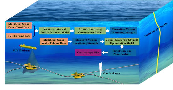
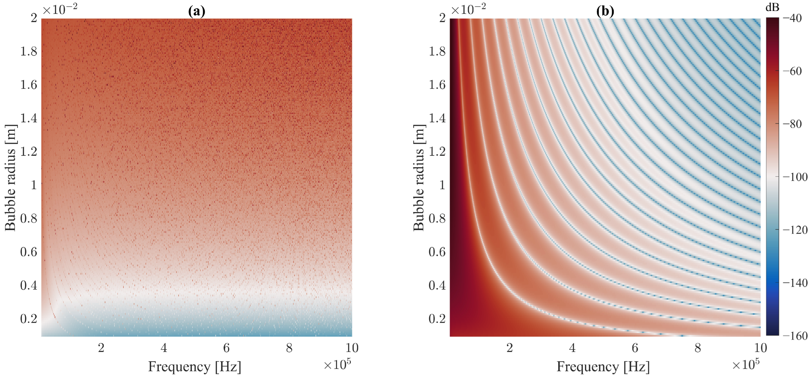
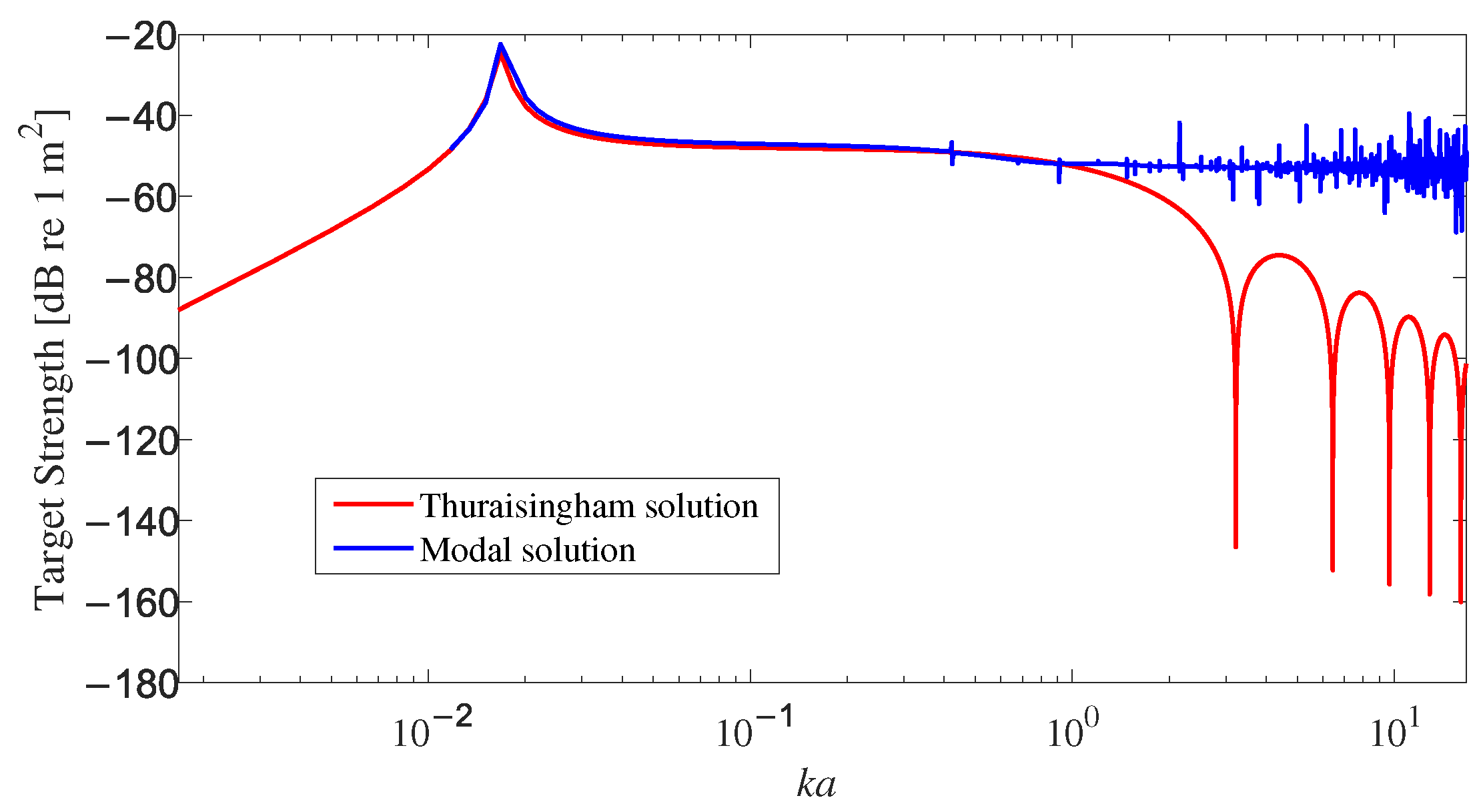
2.1. Volume-Scattering Model of Gas Leakage

Inspired by the work of Ainslie and Leighton [14,28], this study provides a calculation formula of the backscattering cross-section of an individual bubble, which is valid for a wide range of $ka$. This formula is derived by correcting a final factor reported by Thuraisingham [12]. The backscattering cross-section of a single bubble can be expressed by

$${\sigma }_{bs}=\frac{a^2}{{\left({\omega }_0^2/\phantom{{\omega }_0^2{\omega }^2}{\omega }^2-1-2ka{\beta }_0/\phantom{ka{\beta }_0\omega }\omega \right)}^2+{\left(2{\beta }_0/\phantom{{\beta }_0\omega }\omega +ka{\omega }_0^2/\phantom{{\omega }_0^2{\omega }^2}{\omega }^2\right)}^2}\frac{{\left(sinka/\phantom{sinkaka}ka\right)}^2}{1+{\left(ka\right)}^2},$$

(1)

where

$${\omega }_0^2=3\mathrm{Re}\mathrm{\Gamma }\frac{P_{gas}}{{\rho }_{liq}{a}^2}-2\frac{{\tau }_0}{{\rho }_{liq}{a}^3},$$

(2)

$${\beta }_0={\beta }_{th}+{\beta }_{vis},$$

(3)

$$\mathrm{\Gamma }=\frac{\gamma }{1-\left\{\frac{\left(1+i\right)X/2}{tanh\left(\left(1+i\right)X/2\right)}-1\right\}\left(\frac{6i\left(\gamma -1\right)}{X{}^2}\right)},$$

(4)

$$X=\sqrt{\frac{2\omega }{D_p}}a,$$

(5)

Here, a is the bubble radius (m), k is the wavenumber in the water ($\frac{2\pi f}{c}$) (m ${}^{-1}$), f is the echosounder frequency (Hz), c is the speed of the sound (m/s), $\gamma$ is the specific heat ratio of the gas bubble (dimensionless), ${\tau }_0$ is the surface tension of the gas bubbles (N/m), ${\beta }_{th}$ is the viscous damping ($\frac{3P_{gas}}{2{\rho }_{liq}{a}^2\omega }\mathrm{Im}\mathrm{\Gamma }$) (N·s/m), ${\beta }_{vis}$ is the thermal damping ($\frac{2{\mu }_{liq}}{{\rho }_{liq}{a}^2}$) (N·s/m), ${\mu }_{liq}$ is the shear viscosity of the liquid (N/(m·s)), $P_{gas}$ is the pressure of the gas inside the bubble ($P_{atm}+{\rho }_{liq}gd+\frac{2\tau }{a}-p_v$) (Pa), $P_{atm}$ is the atmospheric pressure (Pa), g is the gravitational acceleration (m/s ${}^2$), $p_v$ is the vapor pressure of the water (Pa), d is the water depth at the bubble location (m), ${\rho }_{liq}$ is the water density (kg/m ${}^3$), $\omega$ is the angular frequency (rad/s), $D_p$ is the thermal diffusivity of the gas in a bubble ($\frac{K_{gas}}{{\rho }_{gas}{C}_p}$) (m/s), $K_{gas}$ is the thermal conductivity of the gas in a bubble (W/(m·k)), ${\rho }_{gas}$ is the gas density ($\frac{M_m}{RT}{P}_{gas}$) (kg/m ${}^3$), $C_p$ is the specific heat capacity of the gas at a constant pressure (kJ/(kg K)), $M_m$ is the molar mass of the gas (kg/mol), R is the gas constant (m ${}^2$ kg s ${}^{-2}$ K ${}^{-1}$ mol ${}^{-1}$), and T is the temperature (K).

The backscattering cross-section is typically expressed in decibels, and the backscattering cross-section of a single bubble can be expressed as a target strength as follows:

$$TS=10{log}_{10}\left({\sigma }_{bs}\right)\left(dBre1m^2\right).$$

(6)

Figure 1a shows a resonance peak when $ka\ll 1$, where it can be seen that the target strength first reached its maximum, then started to decline, and after that increased again. This is consistent with the variational tendency of the target strength at the acoustic frequency in the range of 10–400 kHz, as shown in Figure 2a. As shown in Figure 2a, when the acoustic frequency was in the range of 0.5–1 MHz, the $ka$ value approached one, so the first resonance peak was missed. When $ka>1$, the changing trend of the target strength entered a continuous period of oscillatory decline, as shown in Figure 1b. This explains the phenomenon of multiple stripes existing in Figure 2b, representing the target strength alternately rising and falling.

The accuracy of this solution is reduced to the case where $ka>1$. Therefore, this study uses the modal solution presented by Anderson to model the backscattering cross-section of a single bubble precisely for $ka>1$ [29]. In addition, the formulation used by Berges [18] is adopted, and the backscattering cross-section is given by

$$\overline{{\sigma }_{bs}}={\left|\zeta \right|}^2,$$

(7)

where

$$\zeta =\frac{ia}{ka}\sum _{l=0}^{\infty }{(-1)}^l(2l+1)D_l,$$

(8)

$$D_l=\frac{j_l^{\prime }\left(k_{g}a\right)j_l\left(ka\right)-g_{\rho }{h}_c\times j_l\left(k_{g}a\right)j_l^{\prime }\left(ka\right)}{j_l^{\prime }\left(k_{g}a\right)h_l\left(ka\right)-g_{\rho }{h}_c\times j_l\left(k_{g}a\right)h_l^{\prime }\left(ka\right)},$$

(9)

where the meaning of the parameters is as follows:

• $g_{\rho }$: Density ratio of a gas bubble and water ($\frac{{\rho }_g}{{\rho }_l}$) (dimensionless);
• $h_c$: Sound speed ratio of a gas bubble and water ($\frac{c_g}{c_l}$) (dimensionless);
• $k_g$: Wavenumber in a gas bubble ($\frac{{\omega }_g}{c_g}$) (m ${}^{-1}$);
• $j_l$: The spherical Bessel function of the first kind;
• $h_l$: The spherical Hankel function of the first kind;
• $j_l^{\prime }$: The derivative of the spherical Bessel function of the first kind;
• $h_l^{\prime }$: The derivative of the spherical Hankel function of the first kind.

The target strength of a single gas bubble calculated by the modal and Thuraisingham solutions is shown in Figure 3. In Figure 4, the modal solution did not consider the bubble damping effects, and it had low precision for $ka\ll 1$. However, the accuracy of the modal solution decreased for $ka>1$. In this paper, the modal solution is used to model the backscattering cross-section of a gas bubble for $ka>1$, and for $ka\ll 1$, Equation (1) is used to ensure model accuracy.

The target strength has been commonly used to describe the backscattering of a single bubble, while for a bubble population with a wide range of radii, the volume backscattering strength should be used. It should be noted that for multiple discrete bubbles, the multiple scattering effects between bubbles can be ignored [16]. Therefore, the total backscattering value is contributed by all bubbles individually and can be expressed as the volume backscattering coefficient $s_v$ as follows:

$$s_v=\int {\sigma }_{bs}n\left(a\right)da,$$

(10)

where $n\left(a\right)$ denotes the density of gas bubbles with different radii per unit volume.

According to Equation (10), the volume backscattering coefficient is mainly controlled by the gas bubble size distribution and the backscattering cross-section of a gas bubble. Furthermore, the volume backscattering coefficient of multiple discrete bubbles can be expressed as the volume backscattering strength [16] as follows:

$$S_v=10{log}_{10}\left(s_v\right)\left(dBre1m^2\right).$$

(11)

Thus, once the bubble size distribution is determined, the volume backscattering strength can be estimated by Equation (11).

2.2. Bubble Size Distribution Estimation Model

The detection and quantitation of undersea gas leakage are highly dependent on the gas bubble size and rising velocity. Therefore, the determination of these parameters for a given bubble volume is important for both the volume-scattering strength calculation and the gas flux quantitation.

In the literature, there have been several approaches for bubble rising velocity calculation [30,31,32,33]. However, most of them can determine only the rising velocity of bubbles without defining their shapes, such as a sphere, an ellipsoid, or a spherical cap. It should be noted that the bubble shape constantly changes during undersea gas leakage and can also be irregular. To overcome the mentioned shortcoming, this paper derives a simple general formula for the gas bubble’s rising velocity calculation as a function of the volume-equivalent bubble diameter, and it can be expressed as follows [34]:

$$v_{b,general}=\frac{1}{\sqrt{\frac{144{{\mu }_{liq}}^2}{g^2{{\rho }_{liq}}^2{d_e}^4}+\frac{{{\mu }_{liq}}^{4/3}}{0.0208g^{5/3}{{\rho }_{liq}}^{4/3}{d_e}^3}+\frac{1}{2.14{\tau }_{liq}/{\rho }_{liq}{d}_e+0.505g{d}_e}}},$$

(12)

where $d_e$ is the volume-equivalent diameter of a bubble and ${\tau }_{liq}$ is the surface tension of a liquid medium.

In Figure 5, the bubble’s rising velocity values for three bubble shapes (i.e., sphere, spheroid, and spherical cap) are presented. The simple general shape, which is calculated by the general formula and represents a function of the volume-equivalent bubble diameter, is provided for the purpose of comparison. The advantage of the general formula is that it does not require prior knowledge of bubble shape. Therefore, it was not necessary to consider the shape change of a bubble during its rising process. In the test conditions without optical equipment or with inapplicable optical equipment, it is convenient to estimate the bubble radius.

To estimate the rising velocity of a gas bubble, this study adopts the slope angle and the measured sea current speed. It is assumed that the gas plume rises at a constant angle and that the horizontal displacement of gas leakage is dependent only on the sea current. The slope angle is obtained using the height and extent of the gas leakage, and it is calculated by

$$tan\theta =\frac{X_v}{X_h}=\frac{v_v}{v_h},$$

(13)

where $X_v$ and $X_h$ are the vertical and horizontal displacements, respectively, $v_h$ is the horizontal velocity (the current), and $v_v$ is the rising velocity of the gas leakage.

The rising velocity of the gas leakage can be obtained by Equation (13), and the radius distribution of the gas leakage can be estimated by Equation (12).

2.3. Volume-Scattering Strength of a Gas Leakage Measured by Multibeam Sonar

Due to the complexity of an underwater acoustic environment and a multibeam sonar system, the measurement of the volume-scattering strength of gas bubbles is affected by a number of factors. In this paper, the measured volume-scattering strength ($S_v$) of gas bubbles is inferred by the sonar equation with the measured sonar data [35]. For the volume scatters, the received echo level ($EL$) can be approximated as follows:

$$EL=SL-2TL+S_v+10{log}_{10}V,$$

(14)

where $SL$ is the calibrated multibeam sonar source level, $S_v$ is the measured volume-scattering strength, V is the volume ensonified by the transmitted pulse in the receiving beam, and $TL$ is the one-way transmission loss, which can be calculated by Thorp’s formula [36] as follows:

$$TL=20{log}_{10}{R}_1+\alpha R_1,$$

(15)

where the first term denotes the geometrical losses, the second term represents the absorption loss, $\alpha$ is the absorption coefficient, and $R_1$ is the range of the multibeam sonar, which is determined based on t and $\theta$ using constant gradient ray-tracing techniques.

The volume ensonified by the transmitted pulse in the receiving beam can be calculated from the pulse width of the transmitted signal (${\tau }_1$), the speed of the sound in the water (c), and the effective beam solid angle ($\psi$) as follows:

$$V=\frac{c{\tau }_1}{2}{R}_1^2\psi .$$

(16)

The relationship between the received echo levels ($EL$) and raw WCI sampling am-plitudes ($A_{WCI}$) is defined by the array gain associated with the beam-forming processing, time-varying gain ($TVG$), and a constant calibration factor ($CF$). This relationship is affected by a number of parameters, including the frequency, bandwidth, digital-to-analog converter sensitivity, receiving beam pattern, and transducer aging processes [3], and it can be expressed by

$$A_{WCI}=EL+TVG+DI+CF.$$

(17)

Accordingly, the measured volume-scattering strength ($S_v$) can be obtained from the WCI sampling amplitudes ($A_{WCI}$) as follows:

$$S_v=A_{WCI}-SL+2TL-TVG-DI-CF-10{log}_{10}V.$$

(18)

3. Case Study

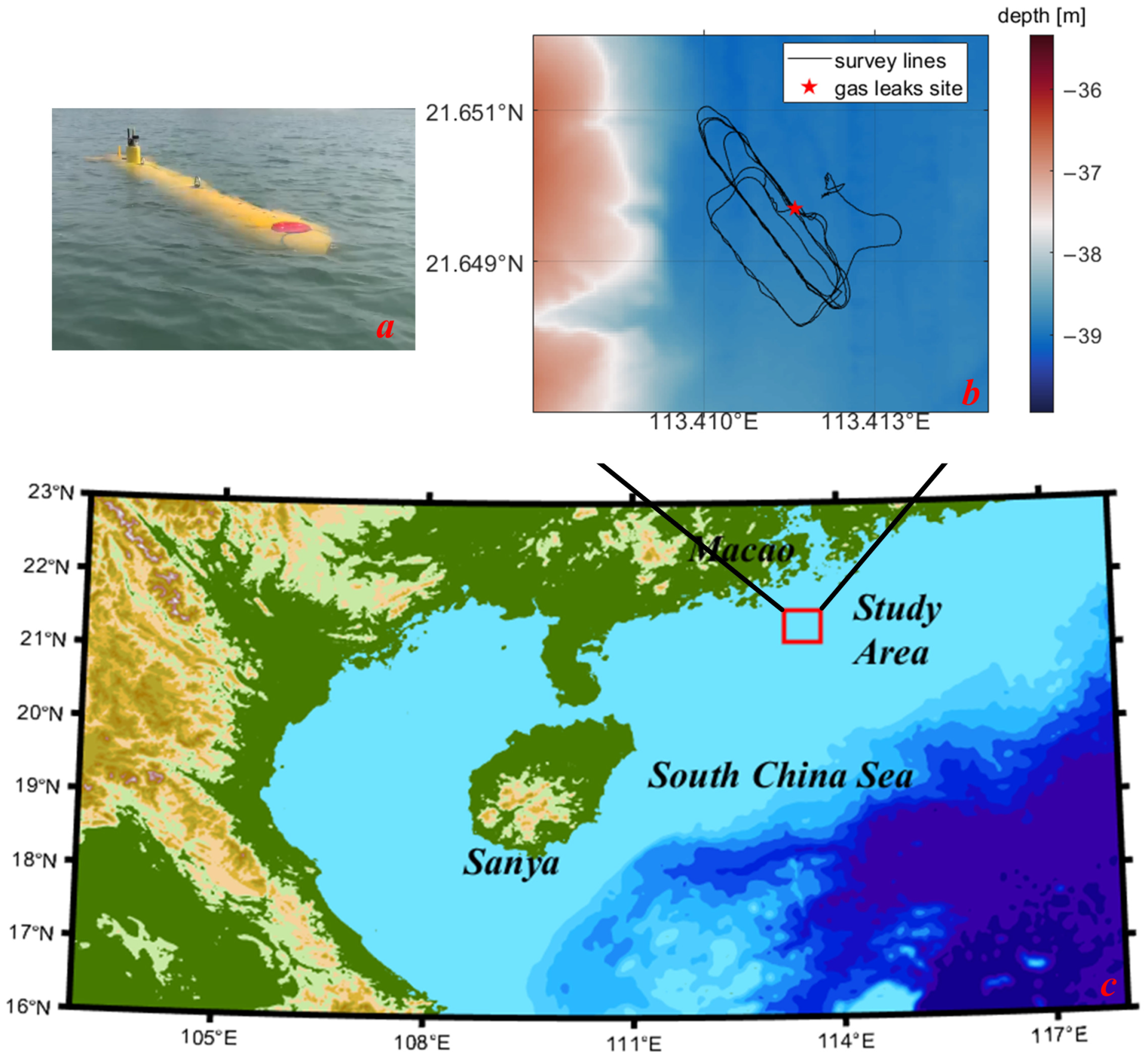
3.1. Field Study Area

The study area was located on the continental slope off China’s shore in the northern South China Sea, as shown in Figure 6c. The water depth in the study region was approximately 35 m–40 m. The gas leakage device was positioned on the seabed (${21}^{\circ }{38}^{\prime }58.9^{″}$ N, ${113}^{\circ }{24}^{\prime }39.9^{″}$ E) at a water depth of approximately 37 m. Figure 6b, shows the gas leakage site, marked with a red star. Gas was pumped to the seabed using a gas compressor.

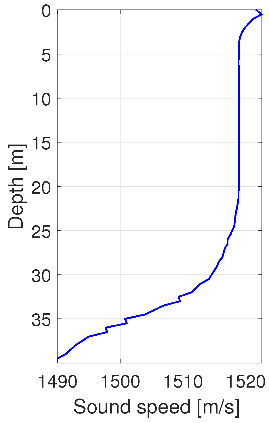
3.2. Data Acquisition and Processing

Acoustic backscattering data were collected by an HT300 QY multibeam sonar developed by Harbin Engineering University in China. The sonar was equipped with an AUV, which was designed to detect subsea pipeline leakages. As shown in Figure 7, it was mounted on the bottom of the AUV during the day survey on 20 August 2020. The multibeam sonar could detect acoustic targets in the water column with a high spatial and temporal resolution over a fan observation area of ${120}^{\circ }$ with a step of $1^{\circ }$. It emitted an acoustic wave with a frequency of 300 kHz and a CW pulse signal with a pulse width of 35 $\mathsf{\mu }$ s. There was a total of 512 beams in the ping fan, and a sampling frequency of 22.22 kHz was used in the beam pattern with a ping rate of 1 Hz. The locations of the detected gas bubbles were accurately determined with a distance resolution of 0.07 m and an angular resolution of $1^{\circ }$, corresponding to at most 0.7 m at the maximum range of 40 m.

The AUV position was recorded by an integrated navigation system, which consisted of the inertial navigation unit (INU), a doppler velocity log (DVL), and a global positioning system (GPS). The positioning accuracy of the integrated navigation system is shown

Table 1. Positioning accuracy of the integrated navigation system.

Integrated Navigation System	Positioning Accuracy
INU + GPS-Assisted	5–15 m
INU + Difference GPS-Assisted	0.5–3 m
INU + RTK Difference GPS-Assisted	0.02–0.05 m
INU + DVL-Assisted	0.2% of the sailing distance

. The sound speed at the depth of the multibeam sonar was measured continuously using the MiniSVS developed by Valeport Company, Totnes, UK. The sound speed profile measured by the RBRconcerto CTD (PBR, Ottawa, ON, Canada) in the study area is presented in Figure 8. The acoustic absorption profile was calculated using the temperature, salinity, and depth data by the empirical formula derived by Wilson [37].

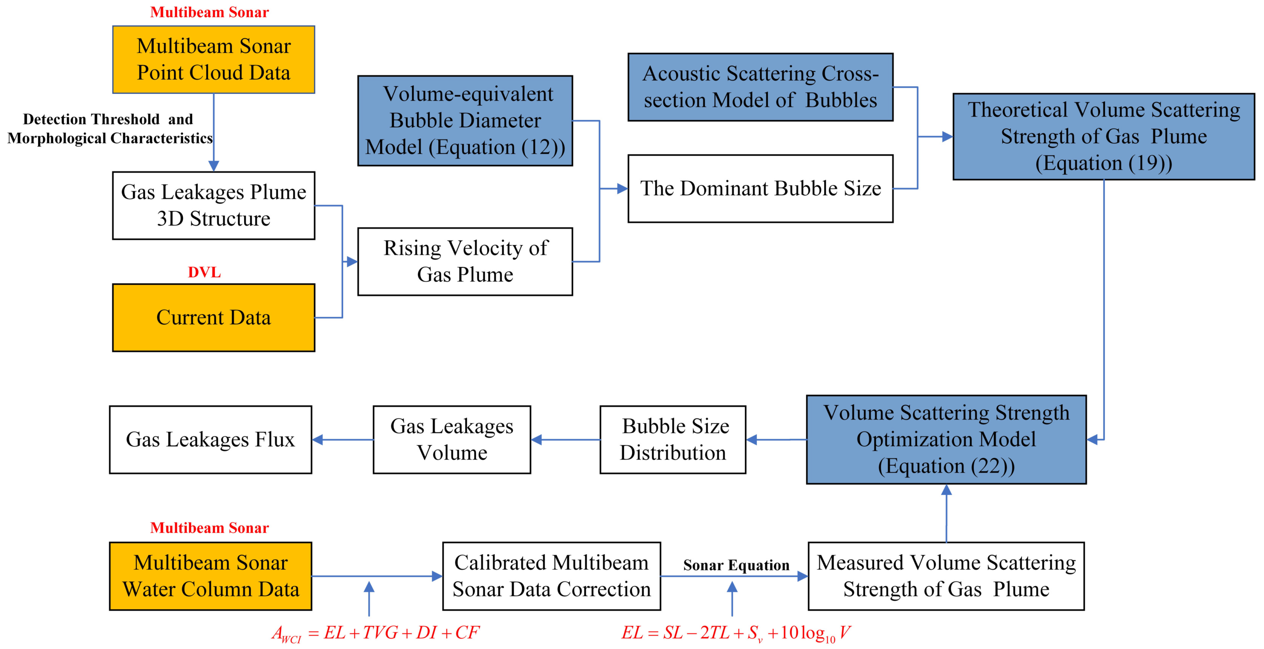
3.3. Gas Leakage Quantitation

The acoustic quantitation flowchart of the gas leakage is shown in Figure 9. The multibeam sonar point cloud data were processed using the detection threshold and morphological characteristics to obtain a 3D structure of the leaking gas plume. Meanwhile, the current data were obtained by DVL. Then, the dominant bubble size was estimated by the volume-equivalent bubble diameter model using Equation (12). By using the acoustic scattering cross-section model of the bubbles, the theoretical volume scattering strength of the gas plume was obtained. In addition, the multibeam sonar water column data and multibeam sonar calibration parameters were used to obtain the measured gas plume’s volumetric scattering intensity with the sonar equation. The theoretical and measured values of the volume-scattering strength were used to construct a volume-scattering strength optimization model. Finally, the bubble radius distribution was estimated, and the leakage flux was quantified.

Assuming that all gas leakage bubbles were of an approximately spherical shape or could be approximated to the spherically shaped bubbles, the contribution of multiple scatterings to the volume scattering of gas leakage bubbles was neglected. Accordingly, the modeled volume-scattering strength of the sample volume was regarded as a sum of single backscattering strengths generated by gas leakage bubbles. The volume-scattering strength obtained from a sample volume was calculated by

$$s_v=\underset{a_1}{\overset{a_2}{\int }}N\left(a\right){\sigma }_{bs}\left(a\right)da,$$

(19)

where a is the bubble radius, ${\sigma }_{bs}\left(a\right)$ denotes the backscattering cross-section of a bubble with a radius a, $N\left(a\right)$ represents the distribution of gas leakage bubbles as a function of the bubble radius, and $a_1$ and $a_2$ are the lower and upper limits of the bubble size distribution, respectively.

For artificial bubble leaks, the bubble size distribution can be approximately parametrized by a log-normal probability density function (PDF) [16], which can be expressed by

$$N\left(a\right)=\frac{1}{a\sqrt{2\pi }\sigma }{e}^{\left[-\frac{1}{2{\sigma }^2}{\left(lna-\mu \right)}^2\right]},a>0,$$

(20)

where

$$\left\{\begin{array}{c}\mu =ln\left[E\left(a\right)\right]-\frac{1}{2}ln\left[1+\frac{D\left(a\right)}{E{\left(a\right)}^2}\right]\hfill \\ \sigma =\sqrt{ln\left[1+\frac{D\left(a\right)}{E{\left(a\right)}^2}\right]}\hfill \end{array}\right.,$$

(21)

where $E\left(a\right)$ represents the expectation for the bubble radius and $D\left(a\right)$ denotes the variance in the bubble radius.

The modeled volume-scattering strength is mainly affected by two parameters ($\mu$ and $\sigma$) in the log-normal probability density function of gas leakage bubble sizes and the total number of bubbles inside the sample volume $N_0$. Therefore, a volume-scattering strength optimization model was constructed to estimate these three parameters. This model is defined as follows:

$$\left[\widehat{\mu },\widehat{\sigma },{\widehat{N}}_0\right]=\underset{\mu ,\sigma ,N_0}{argmin}{∥y-f\left(\mu ,\sigma ,N_0\right)∥}_2,$$

(22)

where $argmin$ is a function that returns the variable value when the objective function reaches the minimum value, y is the measured volume scattering strength, $f\left(\mu ,\sigma ,N_0\right)$ is the modeled volume-scattering strength, and ${\parallel \parallel }_2$ is the $L2$ norm.

The nonlinear least squares problem can be solved by the direct search method or the numerical iterative method. However, since it is challenging to find the gradient of function f, the numerical iterative method could not be used in this study. Thus, the estimated parameters (i.e., $\widehat{\mu }$, $\widehat{\sigma }$, and ${\widehat{N}}_0$) were obtained by the direct search method. The direct search method’s steps were as follows: $\mu$ had a range of 0.1–1.2 in steps of 0.05, $\sigma$ had a range of 0.01–0.4 in steps of 0.01, and the total number of bubbles per volume sampling unit $N_0$ was initialized from the volume of the sampling unit. Next, the three parameters were substituted into Equation (22). Finally, the three estimated parameters, which minimized the objective function, were obtained. Based on the estimated bubble size distribution and the total number of bubbles, the gas leakage volume was approximated to be

$$\widehat{V}=\sum _{j=1}^{N_t}\sum _{i=a_1}^{a_2}\frac{4}{3}\pi N_{ij}{a_{ij}}^3,$$

(23)

where $a_{\left(ij\right)}$ is the bubble radius of size i in the jth sample volume, $a_1$ and $a_2$ are the lower and upper limits of the bubble size distribution, respectively, $N_{\left(ij\right)}$ is the number of bubbles with a radius size i in the jth sample volume, and $N_t$ is the total number of the sample volumes.

Then, the gas flux $\widehat{F}$ (L/min) can be obtained based on the estimated gas leakage volume $\widehat{V}$ and the bubble’s rising velocity $v_v$, which can be calculated by Equation (13) as follows:

$$\widehat{F}=\frac{\widehat{V}}{h_p}\overline{v_v},$$

(24)

where $h_p$ is the height of the gas leakage plume and $\overline{v_v}$ is the mean rising velocity of the bubbles in the plume.

4. Experimental Results and Discussion

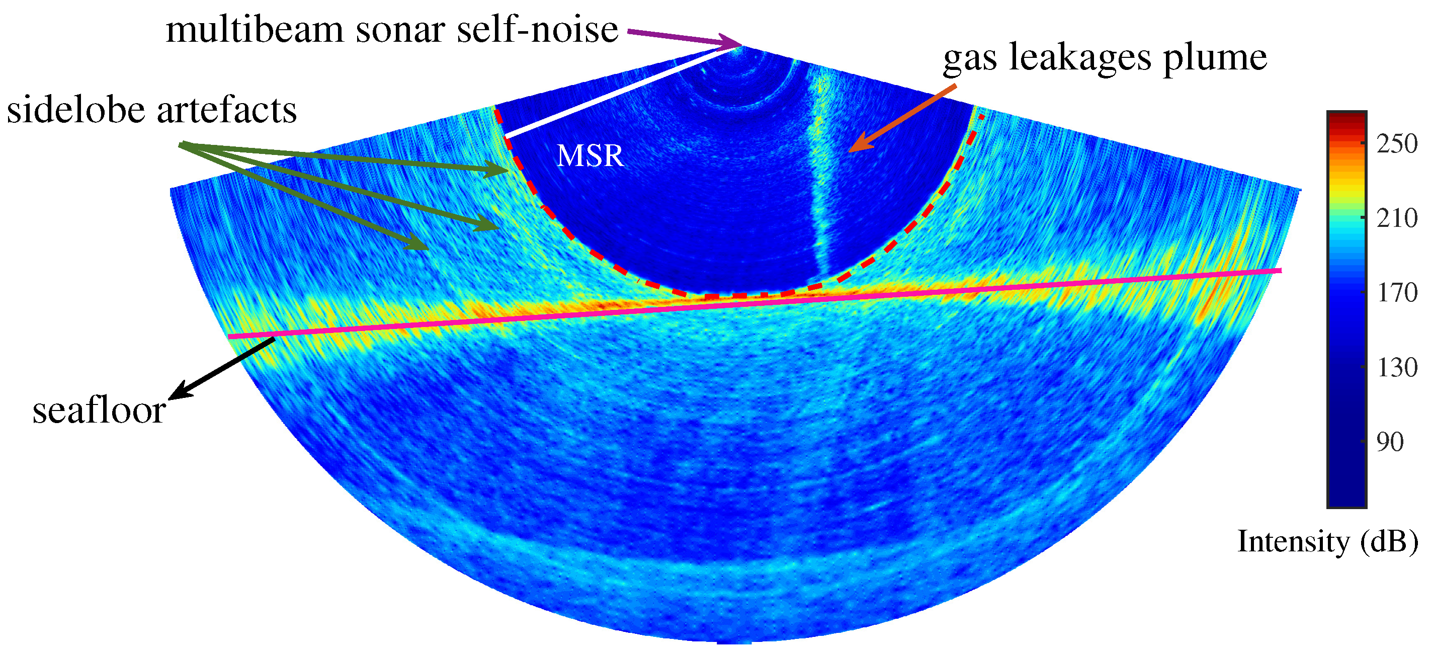
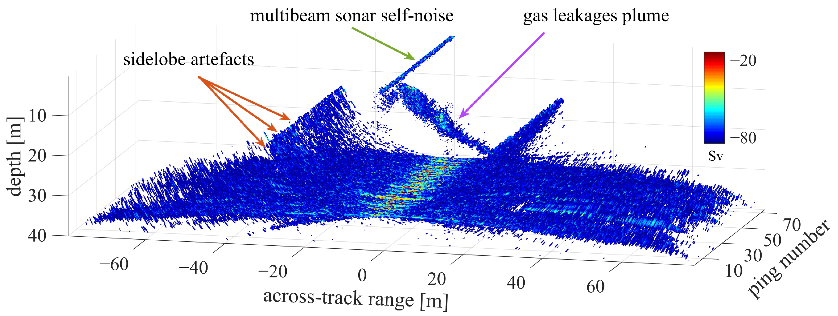
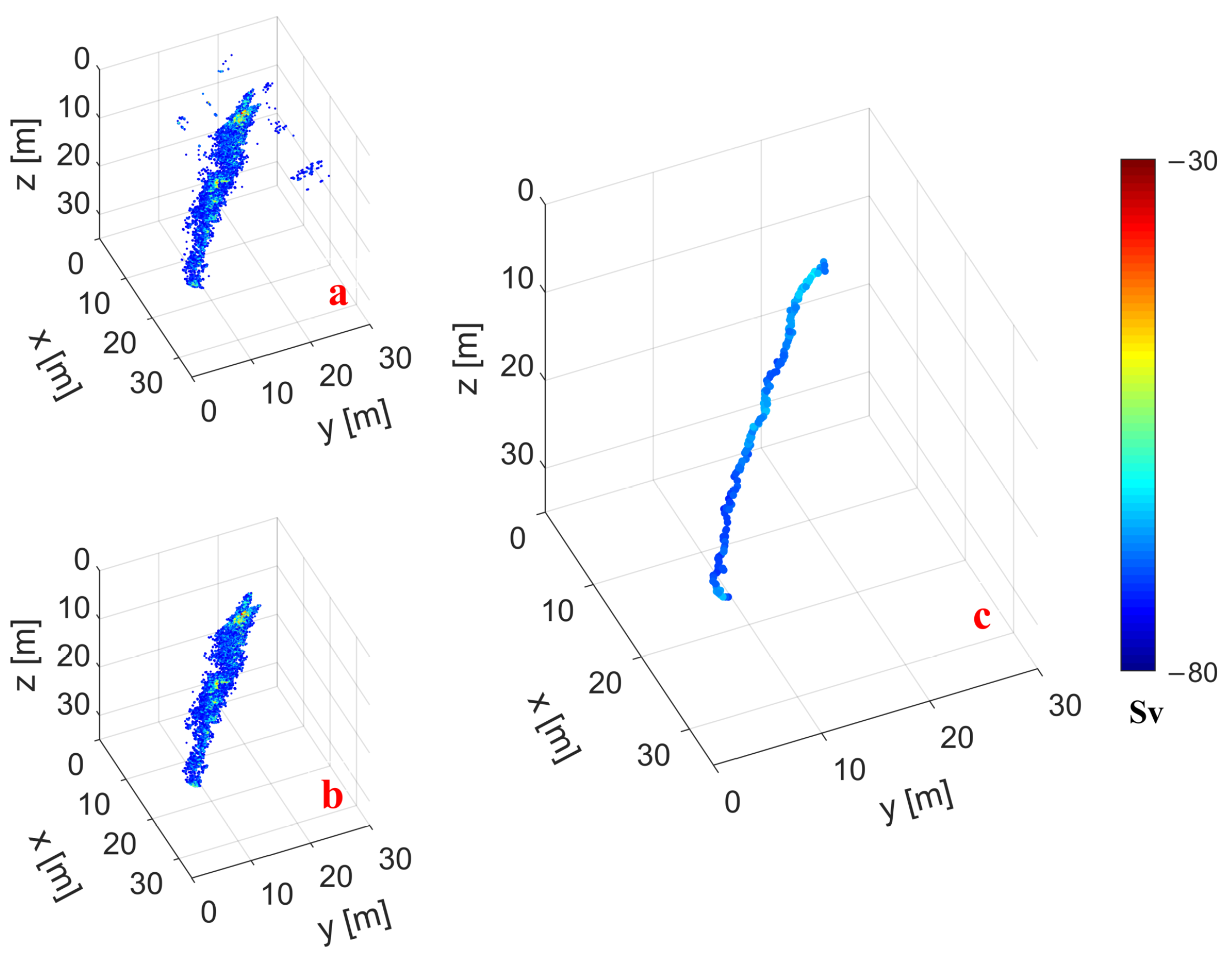
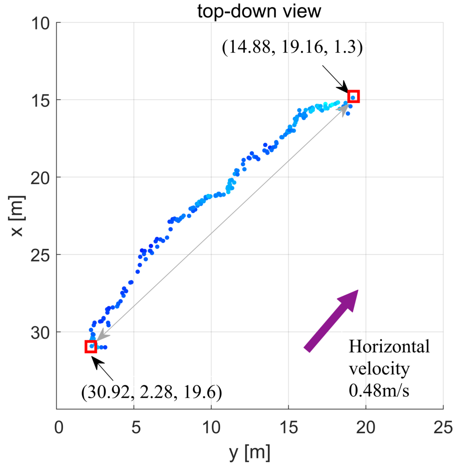
4.1. Gas Leakage Localization

Multibeam data reflecting the gas bubbles that form plume flares in the water column are presented in Figure 10. In the multibeam sonar images, gas leakage usually appears in the flare shape, but noises appear as discrete points. Therefore, the aspect ratio (i.e., the maximum depth extent divided by the maximum extent across the track) of the gas leakage was different from that of the noise or seafloor multiple. Gas leakage usually rises from the seafloor and reaches the surface (in shallow water) or dissolves during the rising process (in deep water) [2]. To distinguish gas leakage from other objects in an underwater environment, such as fish and suspended solids, this study used a specific threshold of $S_v$ inside the selected area and morphological characteristics including the height, width, and aspect ratio. The thresholds of the parameters were selected as follows: height (10–40 m), width (1–2 m), and aspect ratio (5–40). Installation error and motion compensation (pitch, roll, yaw, and heave) were considered during data processing. For each ping multibeam sonar WCI dataset, the detection threshold of the volume-scattering strength and statistical filtering were used to remove the noise and unwanted backscattering from the data. After data cleaning, 3D point cloud data were extracted from 120 consecutive WCIs. Finally, the leakage gas plume was identified.

Using a steered narrow beam of a multibeam sonar allows precise determination of echo sources and therefore provides accurate positioning of the gas leakage site on the seafloor. When the offset of the gas leakage caused by the sea current rises, the gas leakage plume is mostly inclined. Along the AUV track, a detailed 3D multibeam sonar image can be obtained by a sequence of WCIs. As shown in Figure 11, a 3D structure of a gas leakage plume can be reconstructed by clouds of strong scatter points and described in physical terms, such as the position and volume. In addition, sidelobe artifacts and unfiltered noise are also output to the 3D space and appear as strong 3D structures that interfere with the 3D structure of a gas leakage plume. To address this problem, artifacts and noise need to be excluded and removed from the 3D point cloud data. Furthermore, sidelobe-induced interferences can be excluded by eliminating data that have been recorded beyong the minimum slant range (i.e., the shortest radial distance between the multibeam sonar and the seafloor).

As illustrated in Figure 12a, all data beyond the minimum slant range were excluded, and the gas leakage plume could be detected in 3D point clouds. For the 3D point cloud data of the multibeam sonar, the noise points were generally far away from the target point cloud. The distance between the noise point and the neighbor point was larger than the distance between the target point cloud and the neighboring point. Statistical filtering was used to clean the leakage flare, as shown in Figure 12b. Based on the k-nearest neighbor search in the KD tree, each point in the point cloud chose an appropriate neighborhood and computed the average distance from the center point to all neighboring points. Points whose average distances were outside the standard range were defined as outlier noise points and eliminated from the data by statistical analysis, using the global distance as a judging criterion [38]. However, when the acoustic signals of the gas leakage plume were beyond the minimum slant range, the source location of the gas leakage site at the seafloor could not be determined. Therefore, to position the center of the gas leakage accurately, this study sorted the measured volume-scattering strength values of the gas leakage plume, where each layer had a width of 0.2 m. The volume-scattering strength values corresponding to each layer were geometrically averaged to obtain the representative volume-scattering strength value for the strength of the gas leakage. As shown in Figure 12c, the geometric mean was calculated for each set of volume-scattering values for a certain depth range, providing a line with only one position per depth range, which was denoted as the gas leakage spine. The source point of the gas leak can be identified as the lowermost point of the gas leakage spine when it is located just on the seafloor; otherwise, the source point can be estimated by the gas leakage’s spine slope value. A top-down view of the gas leakage spine is displayed in Figure 13. Due to the effect of the sea current, the gas leakage spine was displaced by 23.29 m in the horizontal direction. The average horizontal velocity of the current was measured by the DVL, and it was approximately 0.48 m/s.

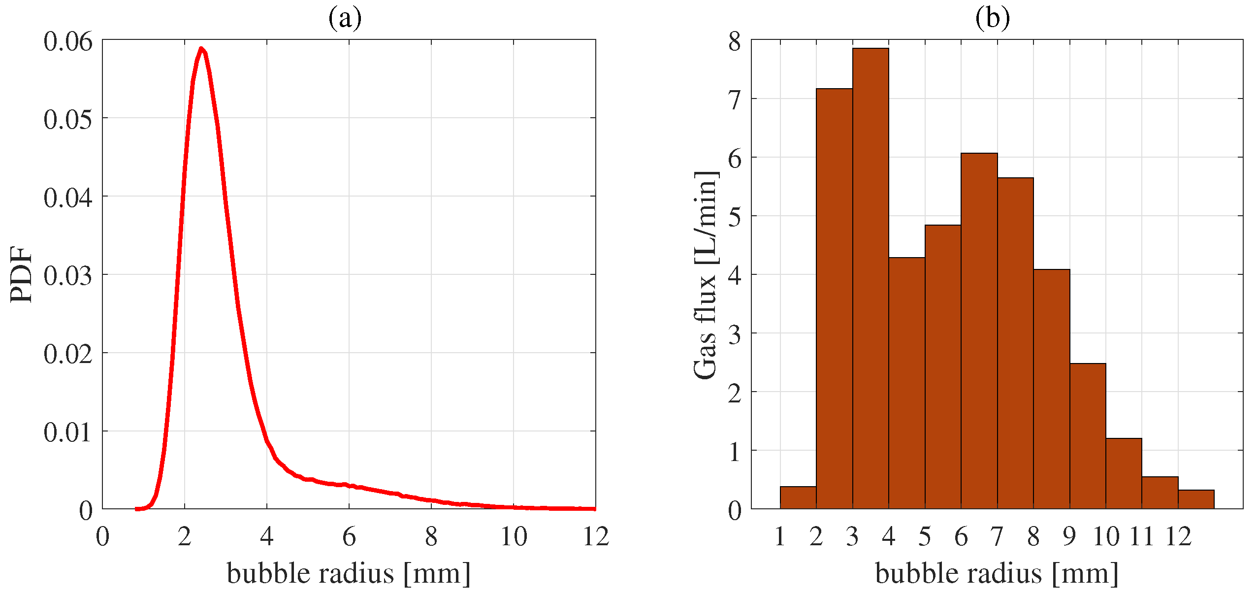
4.2. Bubble Size Distribution

The bubble size distribution is one of the most important factors for quantitating the gas flow rate. Based on the relationship between the upward velocity of the gas leakage plume and the bubble size, the bubble size distribution was determined, and it followed the log-normal distribution. Then, the bubble size distribution was estimated using the volume-scattering strength optimization model.

Due to the influence of ocean currents, bubbles moved laterally through the water column. In the experiment, ocean currents were measured, with the speed varying from 0.32 m/s to 0.61 m/s and having a mean of 0.48 m/s. According to the estimated result of the volume-scattering strength optimization model (Equation (22)), the bubbles in the gas plume had radii ranging from 1 mm to 12 mm with a mean value of 3 mm, as shown in Figure 14a.

4.3. Flow Rate Estimation

Obviously, the gas flux is of primary importance. However, to compute the gas flux, it is necessary to know the depth and volume of a gas leakage plume. Using the water column image data obtained from the multibeam data, the 3D plume was reconstructed.

In this study, the volume of the gas leakage plume was determined using the estimated bubble size distribution. Using the measured depth of the gas leakage plume and horizontal current speed, it was obtained that the gas leakage flux ranged from 29.39 L/min to 56.43 L/min, having a mean value of 44.21 L/min, which was obtained by Equation (24). Due to the constant deflation and inflation process during the operation of the air compressor, the flowmeter value fluctuated between 32 L/min and 67 L/min, having a mean value of 47.34 L/min, which was calculated by the total gas flux and time. The error of the estimated results was −6.61%. The estimated results of the gas flux were roughly in agreement with the experimental data. Additionally, the relative gas flux contribution for each size interval of bubbles was obtained through the calculation of the gas flux for each bubble size interval. As shown in Figure 14b, bubbles with a radius of 2–9 mm accounted for roughly 90% of the gas flux. In particular, bubbles with a radius of 3–4 mm contributed to the gas flux the most, accounting for 17.76%, and they were followed by the bubbles with a radius of 2–3 mm, accounting for 16.21% of the gas flux.

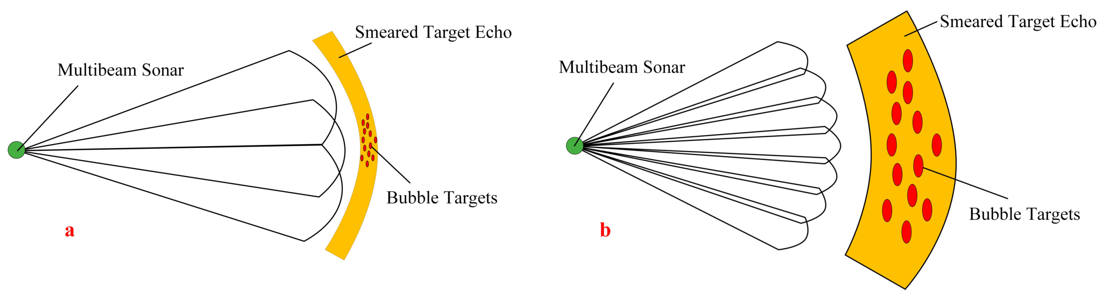
4.4. Seabed Sidelobe Effect and Smearing Effect in Multibeam Sonar

The smearing effect and the seabed sidelobe effect on the estimation of volume scattering strength in multibeam sonar were also analyzed.

For the seabed sidelobe interference, there has been a wide range of high-resolution beam-forming methods, including the multiple signal classification algorithm (MUSIC) [39], the minimum variance distortionless response (MVDR) [40], and their variants [41,42]. These algorithms provide narrow beam widths and low sidelobe levels, which improve interference rejection and enable the detection of targets with small bearing separations. However, they have poor performance in a nonstationary environment [43]. The deconvolved beam-forming algorithm can obtain a high bearing resolution and a low sidelobe [8], but there still will be insufficient or excessive sidelobe suppression. Another method to handle the seabed sidelobe interference is to consider the WCI data only inside the minimum slant range (MSR) [3,44]. However, gas bubbles submerged in the seabed sidelobes cannot be detected through the threshold of the volume-scattering strength. To solve this problem, this study used the aspect ratio to eliminate the effect of seabed sidelobes on the estimation of the volume-scattering strength.

Dinner [45] reported the smearing effect in the school extension measured by multibeam sonar. This scenario is similar to the case considered in this work, where the volume scattering strength of the gas bubbles estimated from multibeam data was biased due to the beam width-related effects. The results indicated that the estimated volume of the gas bubbles increased due to the boundary effects associated with a finite beamwidth. As shown in Figure 15, when a beam partially encountered gas bubbles, the image of the bubbles was spread throughout the beam’s full cross-section. Different from the school targets, in this study, the gas bubbles tended to be partially located within a few beams. This resulted in a smaller measured volume-scattering strength of bubbles, affecting the detection threshold of the volume-scattering strength. Furthermore, since the effect of overlapping beams has been found to be insignificant in practice [46], it is not discussed in this paper.

4.5. Proposed Method Limitations

Recently, methods for monitoring gas leaks from an anthropogenic viewpoint in lakes and oceans have developed significantly in terms of reliability and accuracy. These methods have been applied to both the detection of gas emissions and the quantitation of gas fluxes. It should be noted that optical equipment could not be used in this study because of the turbid water in the South China Sea. The proposed method for gas flow rate quantitation should be validated using a gas collection device and visual measurements. In future works, the effectiveness of the proposed method could be verified for pools or clear lakes.

In the insonified volume unit, echo data of a multibeam sonar are generated considering the contribution of the backscattering produced by several individual targets. A set of assumptions is adopted to develop the proposed method. For the volume-scattering strength, the fundamental assumption is that the total scattered intensity from the insonified volume is equal to the sum of the scattered intensities from each individual target. For gas leakage bubbles, the assumption defining that bubbles are spherical and isotropic scatterers holds. Meanwhile, this study assumed that gas leakage bubbles follow a log-normal distribution. However, these assumptions can lead to large uncertainties because of their idealized real conditions. Still, the acoustic scattering models for irregularly shaped bubbles are very complex. In addition, the shape of the bubbles changes as they rise in the water. It should be noted that without optical equipment, the bubble shape cannot be accurately determined. As a result, it is necessary to simplify the relationship between the bubble shape and the rising velocity by volume-equivalent spherical bubbles. Despite the fact that the proposed method involves simplifications, which can potentially induce uncertainties in the gas leakage flux calculation, it provides a reasonable approximation of the gas leakage flux rate, achieving results that agreed with the experimental results.

5. Conclusions

Gas leakage from pipelines of a realistic size that generate enough bubbles to be observed remotely can be detected and quantitated using multibeam sonar. Mobile platforms equipped with multibeam sonar, such as AUVs, are very convenient for mapping the gas leakage sites and investigating their 3D structures. Compared with other quantitation methods, such as bubble capturing in funnel-like chambers or optical observations, the proposed acoustic quantitation method of the gas leakage plume has important advantages. Namely, remote investigation using an AUV equipped with a multibeam sonar does not disturb the fluid system (e.g., by deploying a heavy device on top of a leak location), and it can investigate a considerably broader region than optical systems.

This study introduces a method for gas leakage plume detection and quantitation based on an AUV equipped with a 300-kHz multibeam sonar. The feasibility of investigating gas leakages using a multibeam sonar was tested in the northern South China Sea. The results show that the escaping gas formed a sloping plume in the water column under the influence of the horizontal ocean current. The presented method employs a volume-scattering strength optimization model to estimate the bubble size distribution. The results indicate that the gas leakage plume radius ranged from 1 mm to 12 mm. In addition, the average leaking gas flux was calculated to be approximately between 29.39 L/min and 56.43 L/min, and it was shown that the bubbles with radii of 3 mm–4 mm contributed the most to the gas flux.

The gas leakage quantitation using multibeam sonar and the proposed method can achieve reasonable gas flux values without any prior knowledge about the bubble size distribution or using a complex scattering cross-section model for irregular bubbles. However, it should be noted that in this study, a simple general multibeam sonar was used. Further improvements could be achieved by observing the shape and behavior of gas bubbles precisely using optical sensors or applying a more accurate multibeam sonar calibration technique fitted to a specific system and natural environment. Furthermore, in future work, a real subsea pipeline leakage detection test could be conducted on the subsea pipeline development demonstration platform of the China National Offshore Oil Corporation. Finally, a real-time detection algorithm could be employed to realize the engineering significance.

References

1. Leighton, T.G.; White, P.R. Quantification of undersea gas leaks from carbon capture and storage facilities, from pipelines and from methane seeps, by their acoustic emissions. Proc. R. Soc. Math. Phys. Eng. Sci. 2012, 468, 485–510. [Google Scholar] [CrossRef]
2. Veloso, M.; Greinert, J.; Mienert, J.; Batist, M.D. A new methodology for quantifying bubble flow rates in deep water using splitbeam echosounders: Examples from the Arctic offshore NW-Svalbard. Limnol. Oceanogr. Methods 2015, 13, 267–287. [Google Scholar] [CrossRef]
3. Urban, P.; Kevin, K.; Greinert, J. Processing of multibeam water column image data for automated bubble/seep detection and repeated mapping. Limnol. Oceanogr. Methods 2017, 15, 1–21. [Google Scholar] [CrossRef]
4. Li, J.; Roche, B.; Bull, J.M.; White, P.R.; Leighton, T.G.; Provenzano, G.; Dewar, M.; Henstock, T.J. Broadband acoustic inversion for gas flux quantification—Application to a methane plume at Scanner Pockmark, central North Sea. J. Geophys. Res. Oceans 2020, 125, e2020JC016360. [Google Scholar] [CrossRef]
5. Zhao, J.; Mai, D.; Zhang, H.; Wang, S. Automatic Detection and Segmentation on Gas Plumes from Multibeam Water Column Images. Remote Sens. 2020, 12, 3085. [Google Scholar] [CrossRef]
6. Xu, C.; Wu, M.; Zhou, T.; Li, J.; Du, W.; Zhang, W.; White, P.R. Optical Flow-Based Detection of Gas Leaks from Pipelines Using Multibeam Water Column Images. Remote Sens. 2020, 12, 119. [Google Scholar] [CrossRef]
7. Minelli, A.; Tassetti, A.N.; Hutton, B.; Pezzuti Cozzolino, G.N.; Jarvis, T.; Fabi, G. Semi-Automated Data Processing and Semi-Supervised Machine Learning for the Detection and Classification of Water-Column Fish Schools and Gas Seeps with a Multibeam Echosounder. Sensors 2021, 21, 2999. [Google Scholar] [CrossRef]
8. Huang, J.; Zhou, T.; Du, W.; Shen, J.; Zhang, W. Smart Ocean: A New Fast Deconvolved Beamforming Algorithm for Multibeam Sonar. Sensors 2018, 18, 4013. [Google Scholar] [CrossRef]
9. Nikolovska, A.; Sahling, H.; Bohrmann, G. Hydroacoustic methodology for detection, localization, and quantification of gas bubbles rising from the seafloor at gas seeps from the eastern Black Sea. Geochem. Geophys. Geosyst. 2008, 9, 1–13. [Google Scholar] [CrossRef]
10. Prosperetti, A. Thermal effects and damping mechanisms in the forcedradial oscillations of gas bubbles in liquids. J. Acoust. Soc. Am. 1977, 61, 17–27. [Google Scholar] [CrossRef]
11. Stanton, T.K. Simple approximate formulas for backscattering of sound by spherical and elongated objects. J. Acoust. Soc. Am. 1989, 86, 1499–1510. [Google Scholar] [CrossRef]
12. Thuraisingham, R.A. New expressions of acoustic cross-sections of a single bubble in the monopole bubble theory. Ultrasonics 1997, 35, 407–409. [Google Scholar] [CrossRef]
13. Medwin, H.; Clay, C.S. Fundamentals of Acoustical Oceanography; Academic Press: Cambridge, MA, USA, 1998; pp. 287–344. [Google Scholar]
14. Ainslie, M.A.; Leighton, T.G. Review of scattering and extinction cross-sections, damping factors, and resonance frequencies of a spherical gas bubble. J. Acoust. Soc. Am. 2011, 130, 3184–3206. [Google Scholar] [CrossRef]
15. Bergès, B.J.P.; Leighton, T.G.; White, P.R. Passive acoustic quantification of gas fluxes during controlled gas release experiments. Int. J. Greenh. Gas Control 2015, 38, 64–79. [Google Scholar] [CrossRef]
16. Leblond, I.; Scalabrin, C.; Berger, L. Acoustic monitoring of gas emissions from the seafloor. Part I: Quantifying the volumetric flow of bubbles. Mar. Geophys. Res. 2014, 35, 191–210. [Google Scholar] [CrossRef]
17. Padilla, A.M.; Weber, T.C. Acoustic backscattering observations from non-spherical gas bubbles with ka between 0.03 and 4.4. J. Acoust. Soc. Am. 2021, 149, 2504–2519. [Google Scholar] [CrossRef]
18. Bergès, B.J.P. Acoustic Detection of Seabed Gas Leaks, with Application to Carbon Capture and Storage (CCS), and lEak Prevention Forthe Oil and Gas Industry. Ph.D. Dissertation, University of Southampton, Southampton, UK, 2015. [Google Scholar]
19. Feuillade, C. Animations for visualizing and teaching acoustic impulse scattering from spheres. J. Acoust. Soc. Am. 2004, 115, 1893–1904. [Google Scholar] [CrossRef]
20. Ryuzo, T.; Koji, I.; Tohru, M.; Yasushi, N. Measurement of Fish School Backscattering Strength Directivity Using Omnidirectional Scanning Sonar. J. Mar. Acoust. Soc. Jpn. 2016, 43, 145–160. [Google Scholar]
21. Kim, H.; Kang, D.; Jung, S.W.; Kim, M. High-frequency acoustic backscattering characteristics for acoustic detection of the red tide species Akashiwo sanguinea and Alexandrium affine. J. Oceanol. Limnol. 2019, 37, 1268–1276. [Google Scholar] [CrossRef]
22. Innangi, S.; Bonanno, A.; Tonielli, R.; Gerlotto, F.; Innangi, M.; Mazzola, S. High resolution 3-D shapes of fish schools: A new method to use the water column backscatter from hydrographic MultiBeam Echo Sounders. Appl. Acoust. 2016, 111, 148–160. [Google Scholar] [CrossRef]
23. Weber, T.C.; Mayer, L.; Beaudoin, J.; Jerram, K.; Malik, M.; Shedd, B.; Rice, G. Mapping Gas Seeps with the Deepwater Multibeam Echosounder on Okecmos Explorer. Oceanography 2012, 25, 54–55, 62, 63. [Google Scholar]
24. Colbo, K.; Ross, T.; Brown, C.; Weber, T. A review of oceanographic applications of water column data from multibeam echosounders. Estuar. Coast. Shelf Sci. 2014, 145, 41–56. [Google Scholar] [CrossRef]
25. Dupré, S.; Berger, L.; Le Bouffant, N.; Scalabrin, C.; Bourillet, J.F. Fluid emissions at the Aquitaine Shelf (Bay of Biscay, France): A biogenic origin or the expression of hydrocarbon leakage? Cont. Shelf Res. 2014, 88, 24–33. [Google Scholar] [CrossRef]
26. Schneider von Deimling, J.; Linke, P.; Schmidt, M.; Rehder, G. Ongoing methane discharge at well site 22/4b (North Sea) and discovery of a spiral vortex bubble plume motion. Mar. Pet. Geol. 2015, 68, 718–730. [Google Scholar] [CrossRef]
27. Weber, T.C. A CFAR Detection Approach for Identifying Gas Bubble Seeps with Multibeam Echo Sounders. IEEE J. Ocean. Eng. 2021, 46, 1346–1355. [Google Scholar] [CrossRef]
28. Ainslie, M.A.; Leighton, T.G. Near resonant bubble acoustic cross-section corrections, including examples from oceanography, volcanology, and biomedical ultrasound. J. Acoust. Soc. Am. 2009, 126, 2163–2175. [Google Scholar] [CrossRef]
29. Anderson, V.C. Sound Scattering from a Fluid Sphere. J. Acoust. Soc. Am. 1950, 22, 426–431. [Google Scholar] [CrossRef]
30. Greinert, J.; Artemov, Y.; Egorov, V.; Batist, M.D.; McGinnis, D. 1300-m-high rising bubbles from mud volcanoes at 2080 m in the Black Sea: Hydroacoustic characteristics and temporal variability. Earth Planet. Sci. Lett. 2006, 244, 1–15. [Google Scholar]
31. Taylor, D.G. The Mechanics of Large Bubbles Rising through Extended Liquids and through Liquids in Tubes. Proc. R. Soc. Lond. 1950, 200, 375–390. [Google Scholar]
32. Grace, J.R. Shapes and velocities of bubbles rising in infinite liquids. Trans. Inst. Chem. Eng. 1973, 51, 116–120. [Google Scholar]
33. Bozzano, G.; Dente, M. Shape and terminal velocity of single bubble motion: A novel approach. Comput. Chem. Eng. 2001, 25, 571–576. [Google Scholar] [CrossRef]
34. Park, S.H.; Park, C.; Lee, J.Y.; Lee, B. A Simple Parameterization for the Rising Velocity of Bubbles in a Liquid Pool. Nucl. Eng. Technol. 2017, 49, 692–699. [Google Scholar] [CrossRef]
35. Urick, R.J. Principles of Underwater Sound, 3rd ed.; Peninsula Publishing: Newport Beach, CA, USA, 1983; pp. 17–28. [Google Scholar]
36. Li, J.; White, P.R.; Bull, J.M.; Leighton, T.G. A noise impact assessment model for passive acoustic measurements of seabed gas fluxes. Ocean Eng. 2019, 183, 294–304. [Google Scholar] [CrossRef]
37. Wilson, W.D. Equation for the Speed of Sound in Sea Water. J. Acoust. Soc. Am. 1960, 32, 1357. [Google Scholar] [CrossRef]
38. Ren, Y.; Li, T.; Xu, J.; Hong, W.; Zheng, Y.; Fu, B. Overall Filtering Algorithm for Multiscale Noise Removal From Point Cloud Data. IEEE Access 2021, 9, 110723–110734. [Google Scholar] [CrossRef]
39. Schmidt, R. Multiple emitter location and signal parameter estimation. IEEE Trans. Antennas Propag. 1986, 57, 276–280. [Google Scholar] [CrossRef]
40. Capon, J. High-resolution frequency-wavenumber spectrum analysis. Proc. IEEE. 1969, 57, 1408–1418. [Google Scholar] [CrossRef]
41. Speiser, J.M.; Bromley, K.; Miceli, W.J. Progress in eigenvector beamforming. Real-Time Signal Process. VIII 1986, 564, 2–8. [Google Scholar]
42. Li, J.; White, P.R.; Bull, J.M.; Leighton, T.G.; Roche, B.; Davis, J.W. Passive acoustic localisation of undersea gas seeps using beamforming. Int. J. Greenh. Gas Control 2021, 108, 103316. [Google Scholar] [CrossRef]
43. Baggeroer, B. Passive sonar limits upon nulling multiple moving ships with large aperture arrays. In Proceedings of the Conference Record of the Thirty-Third Asilomar Conference on Signals, Systems, and Computers, Pacific Grove, CA, USA, 24–27 October 1999; pp. 103–108. [Google Scholar]
44. Hughes Clarke, J.E. Applications of multibeam water column imaging for hydrographic survey. Hydrogr. J. 2006, 120, 3–15. [Google Scholar]
45. Diner, N. Correction on school geometry and density: Approach based on acoustic image simulation. Aquat. Living Resour. 2001, 14, 211–222. [Google Scholar] [CrossRef]
46. Vatnehol, S.; Pena, H.; Ona, E. Estimating the volumes of fish schools from observations with multi-beam sonars. ICES J. Mar. Sci. 2017, 74, 813–821. [Google Scholar] [CrossRef]
Figure 1. Target strength of a single gas bubble under (a) a relatively small k a value and (b) a relatively large k a value.
Remotesensing 14 04301 g001
Figure 2. Target strength of a single gas bubble with a different radius at the acoustic frequency ranging from 10 kHz to 1 MHz: (a) radius of 0.01–0.2 mm and (b) 1–20 mm.
Remotesensing 14 04301 g002
Figure 3. Two solutions used to calculate the target strength of a single gas bubble: (a) modal solution and (b) Thuraisingham solution.
Remotesensing 14 04301 g003
Figure 4. Comparison results of the two models for target strength calculation of a single bubble. It should be noted that multiple scattering between bubbles was ignored, and the volume backscattering strength of the bubbles was contributed by each bubble and computed using Equations (10) and (11).
Remotesensing 14 04301 g004
Figure 5. The rising velocities for bubbles with different shapes.
Remotesensing 14 04301 g005
Figure 6. Study area, equipment, and survey lines. (a) Autonomous underwater vehicle (AUV) equipped with multibeam sonar. (b) Survey lines (black lines) of the AUV in the study area, where the red star indicates the location of the gas leakage site. (c) Position of the study area in the South China Sea, where the red rectangle indicates the multibeam sonar survey area.
Remotesensing 14 04301 g006
Figure 7. A photograph of the HT300 QY multibeam sonar equipped with an AUV.
Remotesensing 14 04301 g007
Figure 8. The sound speed profile measured by the RBRconcerto CTD at the study area in the northern South China Sea.
Remotesensing 14 04301 g008
Figure 9. The gas leakage acoustic quantitation flowchart, where orange blocks represent the input data obtained from the multibeam sonar and doppler velocity log (DVL), and blue blocks denote the applied models.
Remotesensing 14 04301 g009
Figure 10. The water column image obtained by multibeam sonar. A gas leakage plume can be observed in this image, where it appears as a plume flare. The sidelobe artifacts are related to the strong reflection signal from the seafloor, and they affect the gas leakage detection beyond the minimum slant range (MSR). The presented intensities represent uncalibrated relative intensities.
Remotesensing 14 04301 g010
Figure 11. The three-dimensional (3D) point cloud data extracted from 120 consecutive water column images. A 3D gas leakage plume can be observed in this image, and it is tilted due to the horizontal current. The sidelobe artifacts and unfiltered noise also exist in the 3D space, and they appear as strong 3D structures that interfere with the 3D structure of a gas leakage plume. The presented intensities denote relative intensities.
Remotesensing 14 04301 g011
Figure 12. The 3D illustration of the processing steps’ results of the gas leakage flare, where 3D results of the gas leakage flare obtained from (a) uncleaned data, (b) cleaned data, and (c) gas leakage flare spine results calculated by the geometric mean.
Remotesensing 14 04301 g012
Figure 13. A top-down view of the gas leakage spine illustrating the current effect on the horizontal displacement (23.29 m) of bubbles. The average horizontal velocity of the current was measured by the DVL to be approximately 0.48 m/s.
Remotesensing 14 04301 g013
Figure 14. (a) Bubble radius distribution obtained by the volume-scattering strength optimization model. According to the estimation results, the bubble radius was in the range of 1–12 mm. (b) Gas leakage flux results for each bubble radius range. The highest gas leakage flux was contributed by bubbles with a radius from 3 mm to 4 mm.
Remotesensing 14 04301 g014
Figure 15. (a) Smearing effect at long range. Bubble targets were partially located in three adjacent beams, and the echo trace was smeared over the three beams. (b) Smearing effect at short range. Bubble targets were located in several beams and partially in the border beams. The target’s echo was smeared across all beams.
Remotesensing 14 04301 g015