
Shipborne HFSWR Target Detection in Clutter Regions Based on Multi-Frame TFI Correlation

1
College of Engineering, Ocean University of China, Qingdao 266100, China
2
Department of Education, Ocean University of China, Qingdao 266100, China
*
Author to whom correspondence should be addressed.
†
These authors contributed equally to this work.
Remote Sens. 2022, 14(17), 4192; https://doi.org/10.3390/rs14174192
Submission received: 20 July 2022
/
Revised: 23 August 2022
/
Accepted: 24 August 2022
/
Published: 25 August 2022
(This article belongs to the Special Issue Feature Paper Special Issue on Ocean Remote Sensing - Part 2)
Abstract
:High-frequency surface wave radar (HFSWR) is an important marine monitoring technology, and this new regime of radar plays an important role in large-scale, continuous early-warning monitoring at sea. In particular, shipborne HFSWR has wider applications in detecting interesting sea areas, with the advantages of flexible deployment and extended detection capability. Due to the large amount of sea clutter accompanying the echo signals of shipborne HFSWR and the spread of sea clutter due to platform motion, the detection of targets in clutter regions is extremely difficult. In this paper, a multi-frame time-frequency (TF) analysis–based target-detection method is proposed. First, the sea clutter spreading area in the HFSWR echo signal is modeled, and the effects of platform motion and currents on the sea clutter spread are analyzed to determine the sea clutter coverage area; this paper focuses on frequency modeling. Then the TF image (TFI) of each range cell is obtained by TF analysis of the cells within a certain range of the echo signal, and the range cells of possible target points are determined by binary classification of the TFI through a convolutional neural network. Finally, the location of the final target point is obtained by correlation of multi-frame TFIs. Shipborne HFSWR field experiments show that the proposed detection method performs well in detecting targets concealed by sea clutter.
1. Introduction
High-frequency surface-wave radar (HFSWR) plays an important role in marine surveillance and vessel target detection due to its capability for all-weather and large-scale, over-the-horizon monitoring [1]. In comparison with land-based HFSWRs, shipborne HFSWRs offer greater flexibility and a wider detection range. However, the motion of the platform, including six-degree-of-freedom (6-DOF) motion and forward motion, leads to the spread of ship targets and a corresponding broadening of sea clutter in the range-Doppler (RD) spectrum [2], making target detection very difficult.
Walsh et al. [3,4] derived the first- and second-order HFSWR sea surface scattering cross-sectional areas for an antenna mounted on a floating platform under the influence of a wobbling motion. In their simulations, they showed that additional peaks appear in the Doppler spectrum when the antenna is subjected to wobble. Later, Ma et al. [5] analyzed the first- and second-order sea surface scattering cross-sectional areas of HFSWR under the influence of pitch and roll movements of a floating platform and found that the motion-induced peaks appeared symmetrically in the Doppler frequencies. Meanwhile, Yao et al. [6] derived the sea surface scattering cross-sectional area for first- and second-order HFSWR on the basis of a 6-DOF oscillatory motion model. The results showed that 6-DOF oscillatory motions can generate additional symmetrically distributed peaks in the radar spectrum. The location and intensity of these peaks depends on the angular frequency and amplitude of each one-dimensional oscillatory motion. Simulation results in [6] have also shown that the Doppler spectrum expands due to the forward movement of the ship, which is detrimental to target detection. Gill et al. [7] proposed a method based on ocean backscatter for mitigating the effect of antenna motion in the Doppler spectrum of high-frequency radars. Zhang et al. [8] modeled the spatio-temporal distribution of sea echoes from a shipborne radar platform under variable speed and analyzed the relationship between platform velocity and sea clutter propagation. However, the focus of these studies was solving the sea clutter propagation problem, not the target detection problem. In 2021, Yang et al. [9] determined the effects of platform motion and sea current on target echo by modeling and analyzing the effects of platform 6-DOF, forward movement, and sea current on echo delay, and verified the validity of the model through simulation experiments and actual measurement.
Time-frequency (TF) analysis methods in HFSWR target detection have major advantages over traditional CFAR detection and peak detection in terms of accuracy and false-alarm rate. Classical linear methods, such as the short-time Fourier transform (STFT) and wavelet transform (WT) [10], can extend one-dimensional time-series signals to the two-dimensional TF plane, but the TF representations generated by traditional analysis methods are usually ambiguous due to the limitations of Heisenberg’s inaccuracy measurement principle. To overcome the drawbacks of traditional methods, in 2016, Huang et al. [11] proposed the synchrosqueezing transform (SST) based on the STFT and WT for signal redistribution and synchronous compression. Simulations have shown that the synchronous compression transform can improve the resolution of the TF representation, but for linear frequency modulation signals the SST method cannot produce a focused TF representation. Therefore, in 2019 Yu et al. [12] proposed a multisynchrosqueezing transform (MSST) TF analysis method based on the SST, and the simulation showed that although the TF representation was still sufficient in energy after several iterations, it remained limited for more complex cases. Inspired by the SST, in 2017 Yu et al. [13] proposed a TF analysis method based on the STFT post-processing technique, the synchroextracting transform (SET), which compresses all TF coefficients into the instantaneous frequency (IF) trajectory. Unlike the SST compression, the main idea of SET is to retain only the TF information of the STFT results that are most relevant to the time-varying features of the signal, and to remove most of the smeared TF energy, greatly increasing the energy concentration of the new TF representation. In 2021, Cai et al. [14] applied the SET method to the azimuth detection of HFSWR and showed through simulation experiments that the method is significantly better than CFAR detection for improving detection efficiency and reducing directional errors, especially in the case of a low signal-to-noise ratio (SNR).
In terms of target detection, in 2017 Li et al. [15] proposed a TF analysis motion target detection algorithm based on spectral refinement and wavelet-scale rearrangement. The simulation and experimental results showed better detection for vessel targets with small differences in Doppler frequencies and for targets near sea clutter. Chen et al. [16], also in 2017, proposed a two-dimensional multi-signal classification method based on sparse recovery to improve the target-detection capability of HFSWR. The above methods all detect targets away from sea clutter or near its edges. In 2018, Wang et al. [17] proposed a method for detecting targets within the sea clutter zone using in situ sea state information, but this was shown through experiments to be useful for target detection only in specific scenarios. In 2021, Wu et al. [18] proposed an algorithm for target detection under the occlusion of strong clutter and a complex interference environment, which uses a Faster R-CNN network to localize the clutter and interference region and then a two-stage cascade algorithm to detect the region. Experiments have shown that the method has good results for detecting targets obscured by clutter and interference areas, but its performance degrades when detecting targets completely obscured by sea clutter.
The aim of this paper is to establish a platform-motion model to mathematically analyze the effects of platform motion on echo signals and to focus mainly on the sea clutter spreading in order to locate the target in the sea clutter coverage area for the next step. Both simulations and field experiments verified the validity of this model. One TFI is obtained by using the SET on the clutter region, and a convolutional neural network (CNN) is designed to bifurcate the TFI to obtain the location of the suspected target. Eventually, the exact location of the target is determined by multi-frame correlation.
The structure of this paper is as follows. Section 1 gives a brief introduction to the existing research results related to this paper. In Section 2, the differences between shore−based HFSWR and shipborne HFSWR are compared, and the difficulties of shipborne HFSWR in the target side are pointed out. At the same time, the process framework of this article is given. In Section 3, we model the frequency direction of the HFSWR on the ship platform, and carry out theoretical analysis and finally obtain the sea clutter widening area. In Section 4, the time-frequency analysis is carried out according to the sea clutter broadening area determined in the previous section, and the TF map is classified by CNN to obtain the classification results. Section 5 uses the multi-frame correlation method to remove the false alarm target and the exact position of the real target point. Finally, Section 6 gives the conclusion.
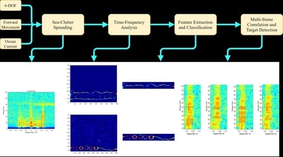
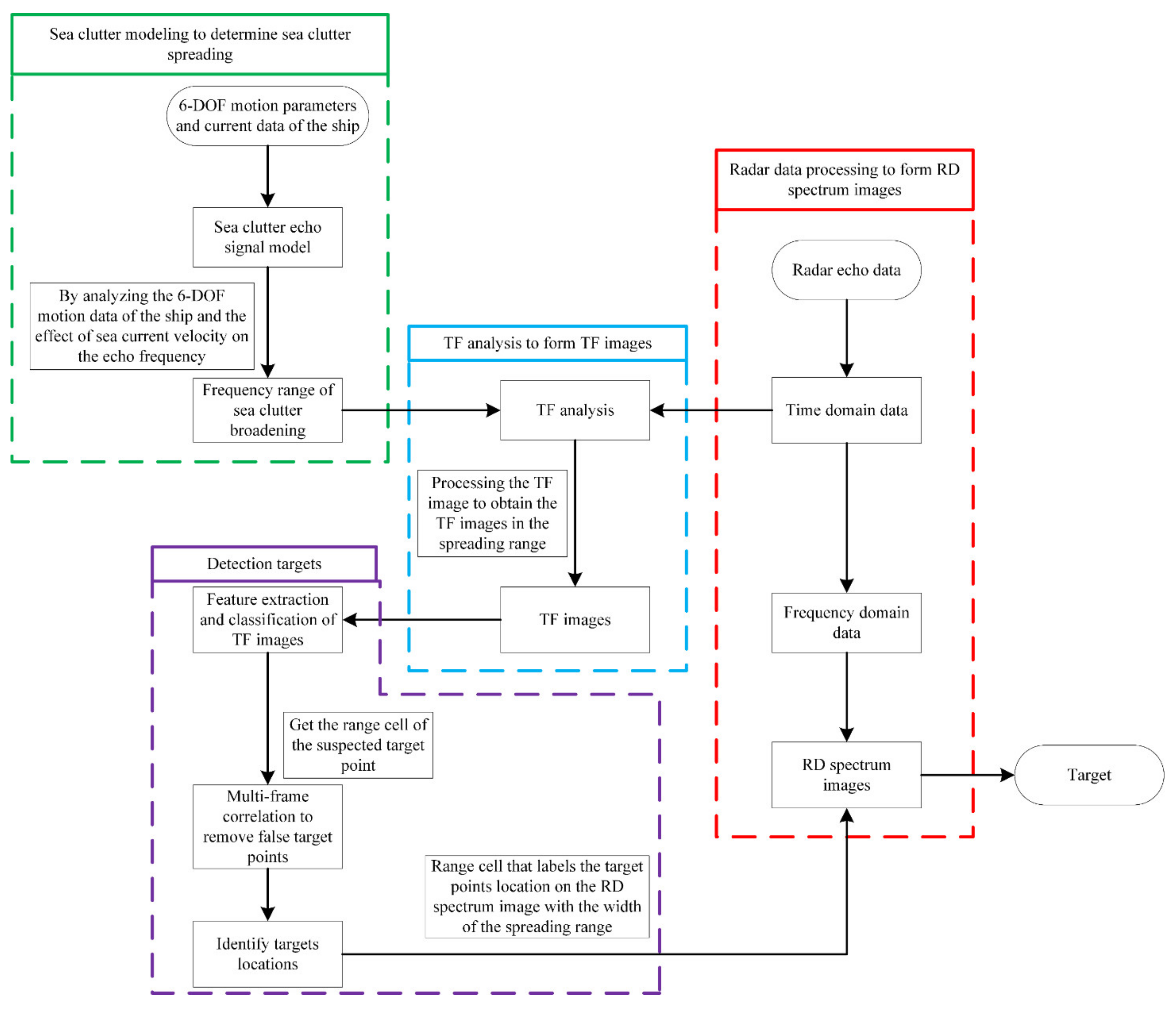
2. Detection Framework
2.1. RD Spectrum of Shipborne HFSWR
The HFSWR echo signal contains signals reflected from vessels along with clutter and interference, including sea clutter, radio-frequency interference, ionospheric clutter, and ground clutter. For shore−based HFSWR, the ground clutter is easy to deal with, as it is at zero frequency. For shipborne HFSWR, the ground clutter is greatly expanded and shifted, which makes target detection difficult. Furthermore, the sea clutter is obviously expanded in the RD spectrum, causing more targets to be submerged in clutter, and the SNR of the echo signal decreases sharply. Therefore, the accuracy of target detection decreases significantly in this situation, and a new detection method for targets concealed in clutter is needed, which is great importance in HFSWR applications.
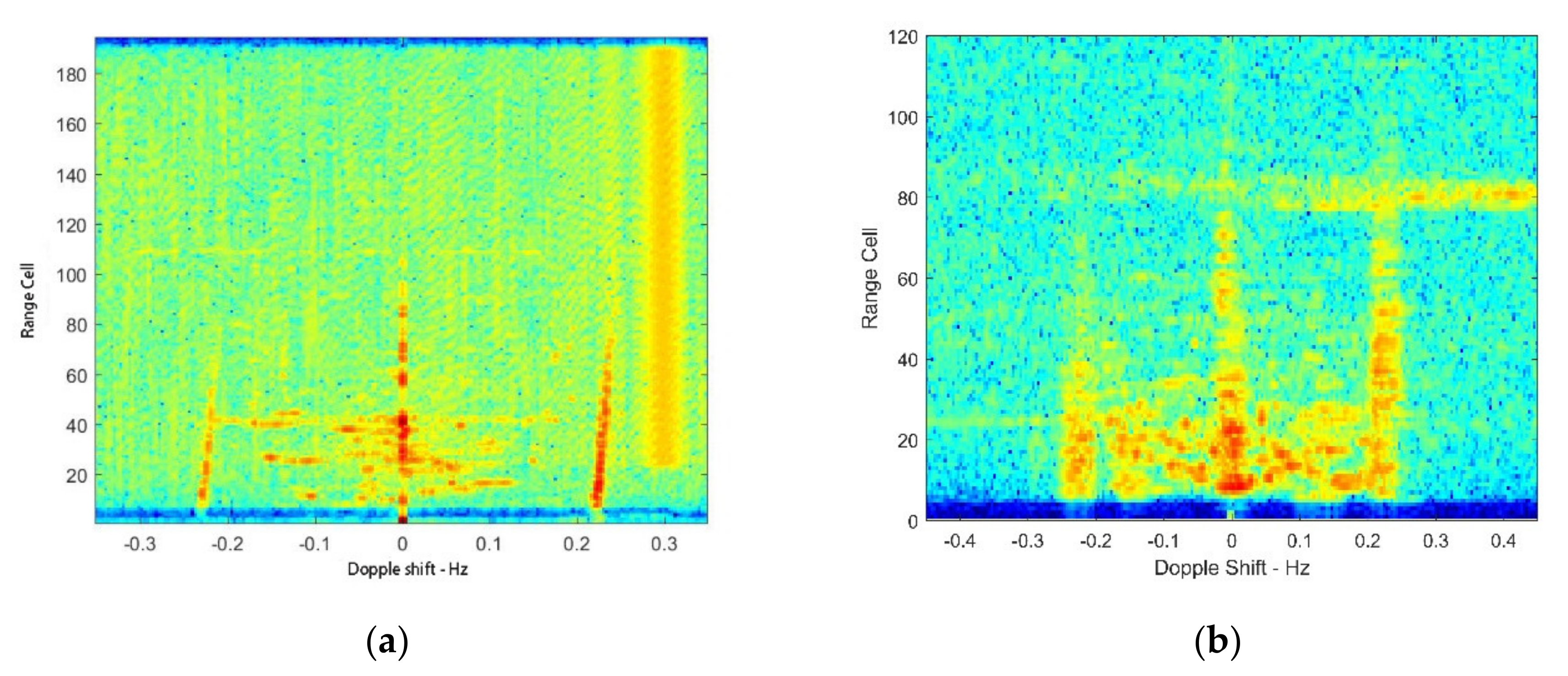
In comparison with land-based HFSWR, the first-order sea clutter region of shipborne HFSWR is significantly wider due to the influence of platform movement and the current, resulting in an increased coverage area, which makes it more difficult to detect targets in the region. Figure 1 shows the RD spectrum of HFSWR. It can be seen that the first-order sea clutter broadening is serious, and the interference signal also appears at the edge of the broadening, so this paper first determines the sea clutter broadening range by theoretical derivation to make the detection of targets concealed in first-order sea clutter feasible.
2.2. Detection Framework
From Figure 1b, it can be seen that the sea clutter spreading of shipboard HFSWR is serious. In this complex situation, a new detection method of target detection in clutter is proposed with the overall framework shown in Figure 2. First, the sea clutter spreading range under the influence of platform motion is obtained by modeling the floating platform and analyzing its influence on the radar echo signal. Field data experiments have verified the validity of the model, in which the TF spectrum for each range cell can be obtained by TF analysis of the determined sea clutter spreading range. The TFI is sent into the trained CNN to classify the potential positions of the target, and the final position of the target is determined by correlating the multi-frame TFIs.
3. Problem Formulation
3.1. Spreading of Sea Clutter
Shipborne HFSWR emits electromagnetic waves to the sea surface, and these are resonantly scattered by the waves to form a sea surface return spectrum. Under the influence of certain radar system parameters and sea surface factors, a first-order scattering model of the sea surface is constructed. The simulation model of the echo signal of the i-th antenna [19,20] is constructed by considering the effect of the 6-DOF of the platform as follows:
where is the background noise, F is the ground wave propagation attenuation coefficient, is the transmitter power, and are the transmitting and receiving antenna gain, respectively, is the wavelength of the electromagnetic wave emitted by the radar, is the distance, is the first-order scattering cross-sectional area at the sea surface, is the antenna discharge image function, is the guide vector and amplitude of the i-th antenna, and is the orientation range of the target scattering region with respect to the observation point [–90°, 90°].
In Equation (1), the first-order scattering cross-sectional area of the sea surface can be expressed as
where is the Bragg frequency in the simulated echo signal, calculated as follows:
where is the theoretical Bragg frequency, is the frequency effect due to currents, and is the frequency effect due to platform motion.
The antenna pattern function in Equation (1) is given by
where is the number of electromagnetic waves, is the length of the antenna, is the roll angle, and is the pitch angle.
The array steering vector in Equation (1) is calculated as
where the magnitude is normalized. and are calculated as follows:
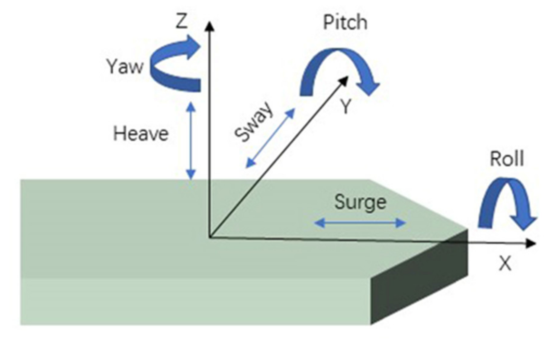
where is the yaw angle, is the distance between the antenna and the platform centerline, is the surge displacement, y is the sway displacement, z is the heave displacement, is the distance from the platform’s center of gravity to its top surface, is the array element spacing, and is the number of array element antennas.
3.2. Modeling of Platform Movement and Motion Due to Ocean Currents
For the generality of the model, a fixed right-handed Cartesian coordinate system is established with the platform’s center of gravity as the coordinate origin O and its forward direction as the x-axis shown in Figure 3. The velocity of the current, the forward movement of the platform, and the velocity in each of the 6-DOF are modeled in Figure 3.
3.2.1. Forward Movement and the Motion from Ocean Currents
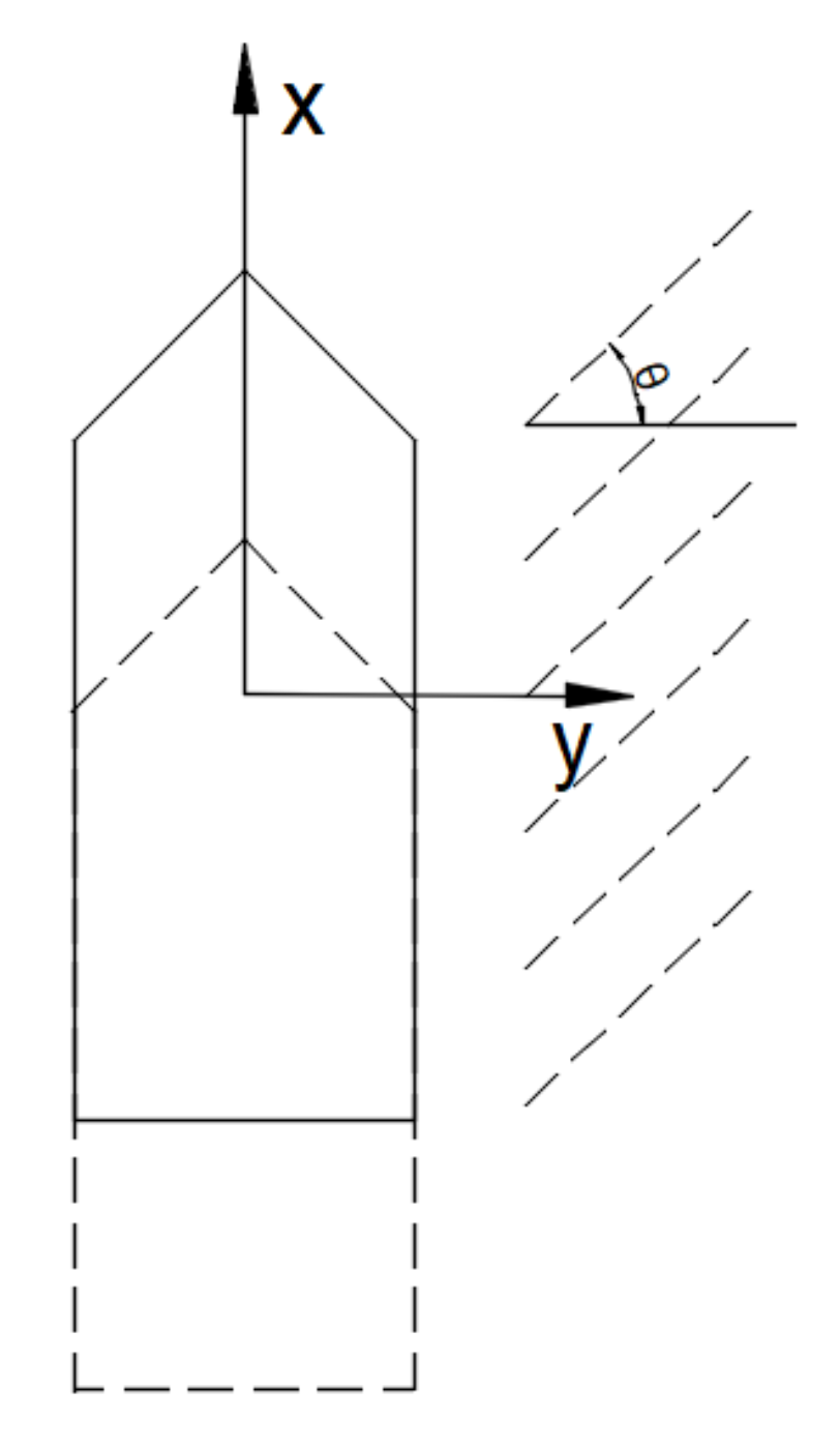
A schematic diagram of the forward movement of the platform and the effect of the current is shown in Figure 4. Let the forward speed of the platform be , the velocity of the current be , and the angle between the direction of the incoming wave and the axis normal to x be . is the angle between the direction of the current and the x-axis. Therefore, the effect of the velocities of the current and the platform’s forward movement on the echo frequency is as follows:
where the speed of the current is obtained by the equipment on board. Because the speed of the platform in the experiment changes relatively slowly, it is approximated by its average speed during that time.
3.2.2. Heave Movement
Droop can be seen as a superposition of sinusoidal motion in the vertical direction. Walsh et al. [3,4] showed that vertical antenna motion does not produce additional Doppler effects because it does not have a component in the direction of wave propagation. Therefore, vertical oscillation has no effect on echo signal frequency.
3.2.3. Sway and Surge Movements
Because the sway and surge movements are translational in the direction of the x- and y-axes, the average velocities of the sway and surge movements are set at and , respectively, and the magnitudes of both can be obtained from the motion data of the platform over a period of time. The effect of sway and surge movements on the echo frequency is therefore as follows:
3.2.4. Roll Movement
The roll movement of the platform can be decomposed into two components, in the directions of y- and z-axes. Because the motion in z-direction has no effect on echo frequency, the effect of the roll movement on the echo frequency is as follows:
3.2.5. Pitch Movement
The pitch movement is synthesized from the movements in the x- and z-directions, so it can be decomposed into movements in those two directions, from which the effect of the echo frequency of the pitch-movement term can be obtained as follows:
3.2.6. Yaw Movement
The yaw movement of the platform can be seen that the bow rocking is a synthesis of movement in the directions of the horizontal x- and y-axes, so the effect of the bow rocking on the echo frequency can be decomposed into those two directions, as follows:
The total effect of the platform’s 6-DOF motion and the currents on the frequency of the radar echo signal are therefore as follows:
Substituting Equation (20) into Equation (3) gives the Bragg frequency in the echo signal , and substituting the Bragg frequency into Equation (2) yields the first-order scattering cross-sectional area of the sea surface in the actual signal.
3.3. Simulation and Verification of Sea Clutter Spreading
To verify the validity of the model, the echo signals were simulated using MATLAB software. The data for the simulation were taken from the ship’s inertial navigation system. The simulation parameters are shown in Table 1, where the velocities of all six degrees of freedom have been replaced by the average velocity over a period of time and the speed of the sea current is obtained by the equipment on board.
4. Time-Frequency Analysis
4.1. Time-Frequency Method
The sea clutter in the spreading range can be further analyzed by using TF analysis. This is an important class of methods for dealing with non-stationary signals in terms of two-dimensional functions of time and frequency. In this paper, the SET is applied as a post-processing method of the STFT and generates a more energetically focused TF representation than the classical TF analysis methods.
A synchronous extraction operator (SEO) is built on top of the original TF representation, calculated with the STFT to extract only the TF coefficients in the instantaneous frequency trajectory. Let the STFT of the input signal be Ge(t, f). Then the SET of the signal can be expressed as follows:
where is the instantaneous frequency of the STFT and is the SEO:
So,
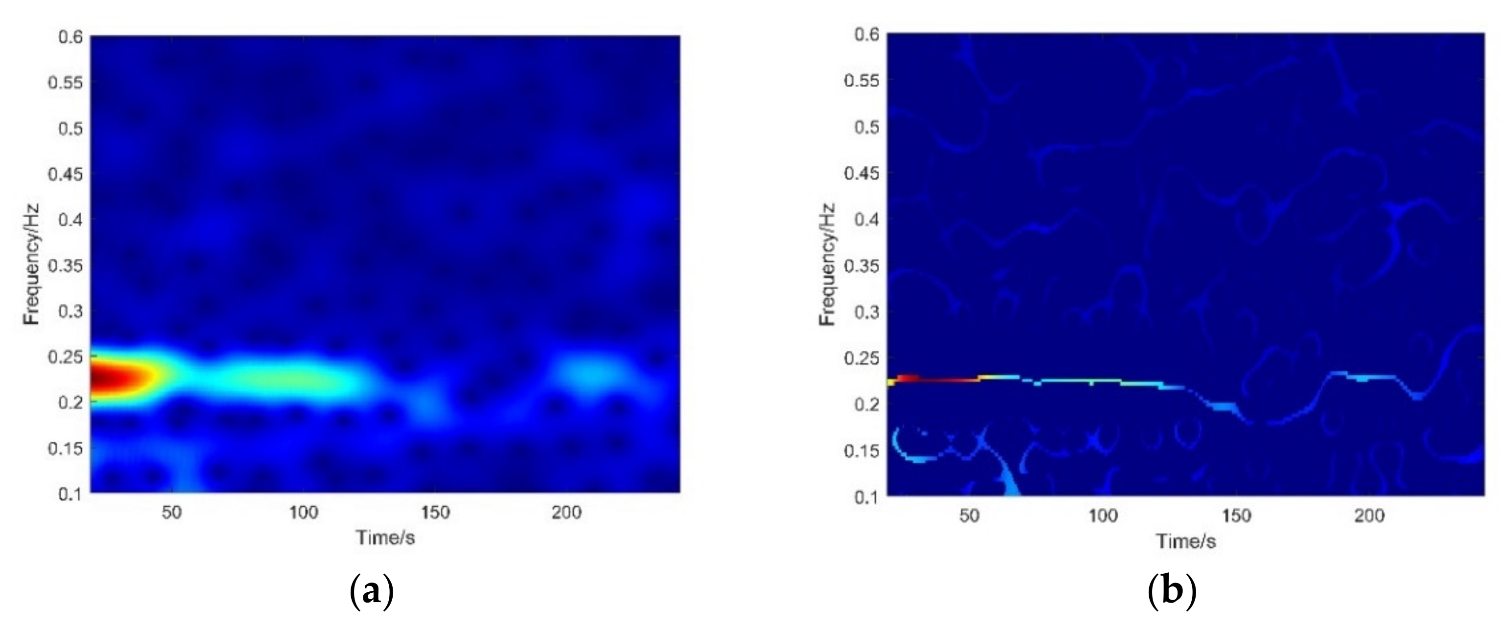
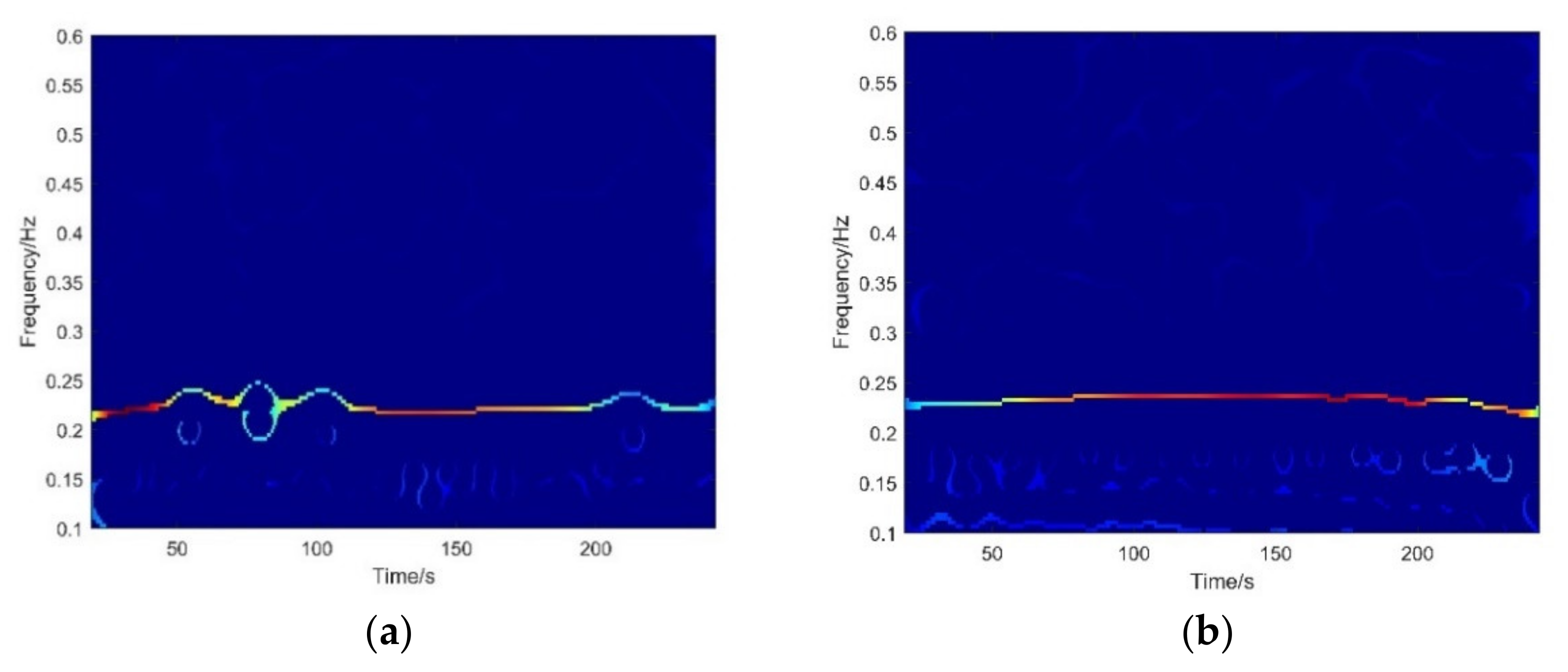
As can be seen from Equation (23), the SEO only performs coefficient extraction on the STFT instantaneous frequency trajectory, which can be more energy focused than the original STFT results, and the resolution of the instantaneous frequencies can be greatly improved, as shown in Figure 6.
If we use a linear frequency modulated interrupted continuous wave (FMICW) signal as an echo signal for an HFSWR, we can think of the radar’s echo signal as a superposition of harmonic signals of multiple frequencies. At the same time, the echo signal usually contains a variety of clutter and interference.
When the input signal contains only sea clutter, as compared to the case when it contains both sea clutter and the target signal, the frequency composition of the echoes will be different. Figure 7 shows the TFI obtained by performing an SET on the radar echo at a certain time.
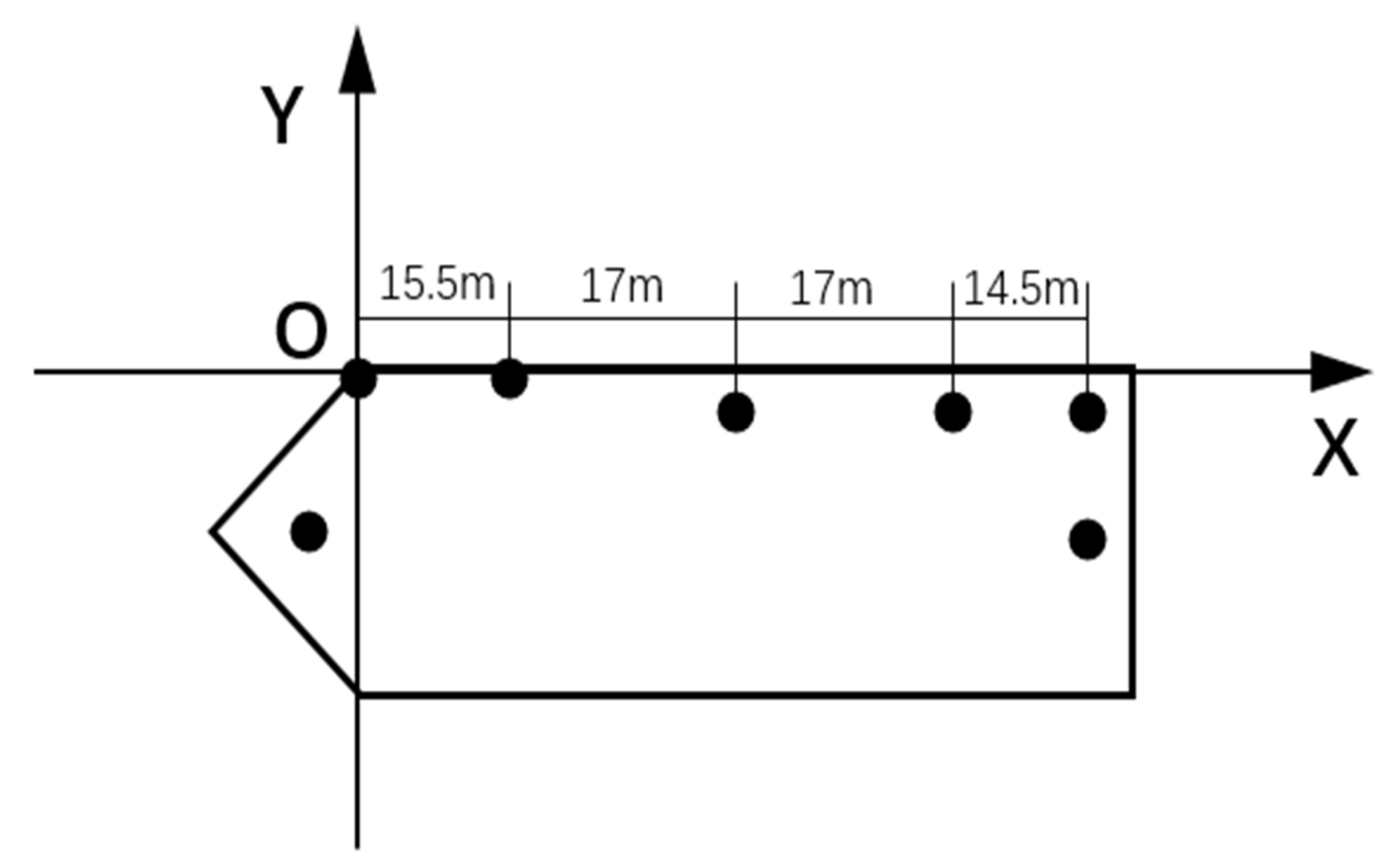
The shipborne HFSWR parameters are shown in Table 3. The antenna array used in the experiment has two transmitting antennas and multiple receiving antennas. In the field shipborne HFSWR experiment, as shown in Figure 8, due to the space restriction on the platform, the antenna array cannot be installed linearly. We establish a coordinate to represent the position of the five antennas. Five receiving antenna placement position coordinates are (0, 0), (15.5, 0), (32.5, 1), (49.5, 1), (64, 1), and the two transmitting antennas are (−3, −1.5), (64, −3). From these coordinates, the steering vector of the non-uniform array can be computed to determine the azimuth of the target.
4.2. Feature Extraction and Classification
In this section, feature extraction and classification are performed for the TFIs of each range cell via the SET method. The neural network chosen is GoogLeNet [21]. In comparison with previous neural networks, such as AlexNet [22] and VGGNet [23], GoogLeNet is the first large-scale CNN formed by stacking inception modules. The GoogLeNet neural network was designed in the dropout layer with a 30% discarding probability due to more distinctive features. Specific details of the auxiliary classifier are as follows: the average pooling layer was designed with a filter size of 5 × 5, a stride size of 1; an output of 14 × 14 × 512 for (4a) and 14 × 14 × 528 for (4d); the fully connected layer with 1024 units and corrected linear activation; the dropout layer with a dropped output ratio of 60%; and the linear layer uses the softmax loss as a classifier. The network structure is shown in Table 4.
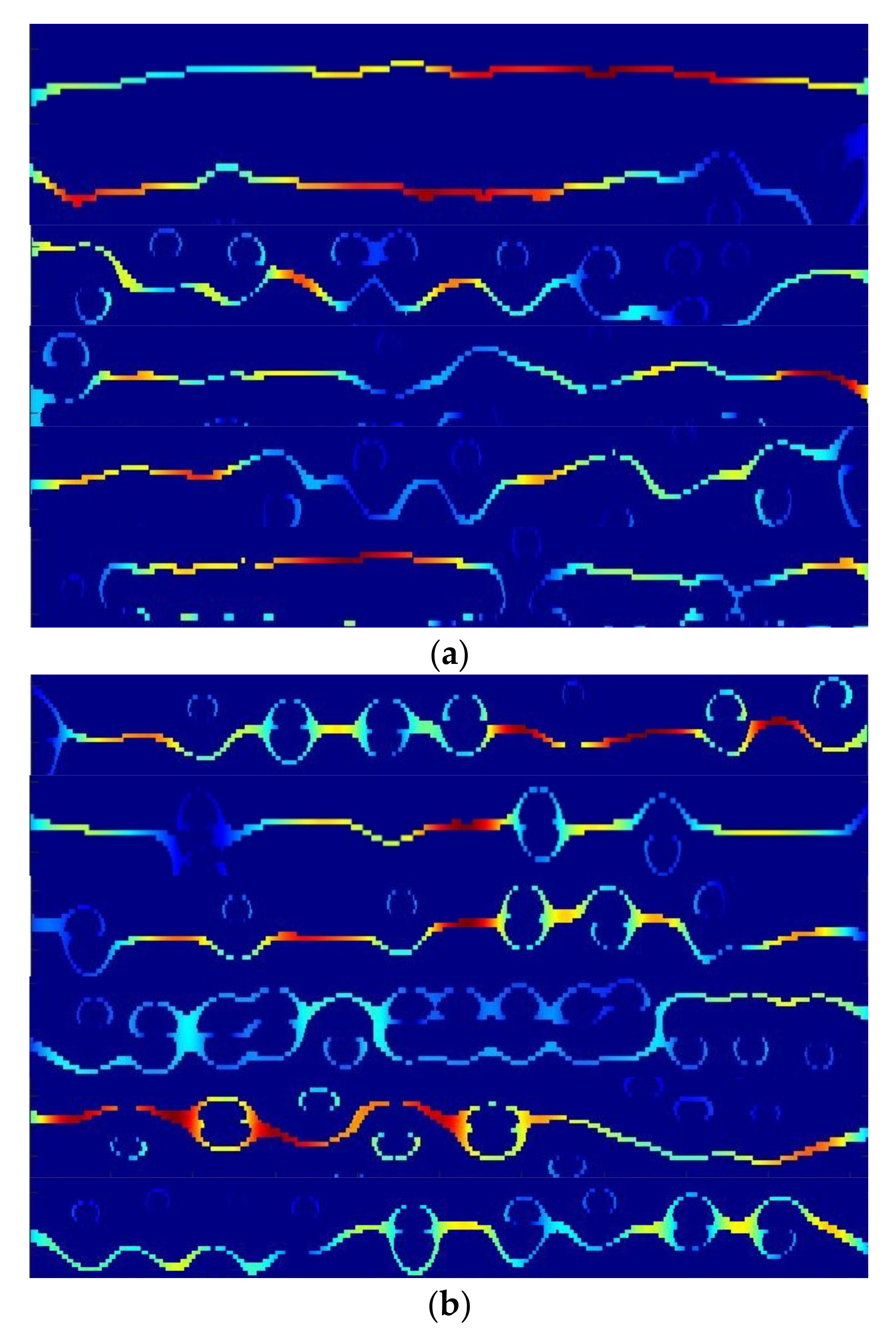
The TF analysis of the HFSWR echo data is performed using the SET to obtain a TFI for each range cell, and the resulting TFI is included for the construction of the dataset. The spread of the target point in the shipborne HFSWR echo signal can lead to features similar to the target point in nearby cells, so attention should be paid to this issue when creating the dataset. The dataset constructed here consists of 1000 pure sea clutter instances and 600 targets with sea clutter. The training and testing samples are split in a ratio of 7:3. The resulting sample dataset is then labeled with two categories: targets with clutter and pure sea clutter, both illustrated in Figure 9. Another batch of data was taken for testing using several CNN models trained to compare the test results, as shown in Table 5. It can be seen that the method used here is more accurate than the AlexNet and VGG-16 networks.
5. Target Detection
5.1. Multi-Frame Correlation and Target Detection
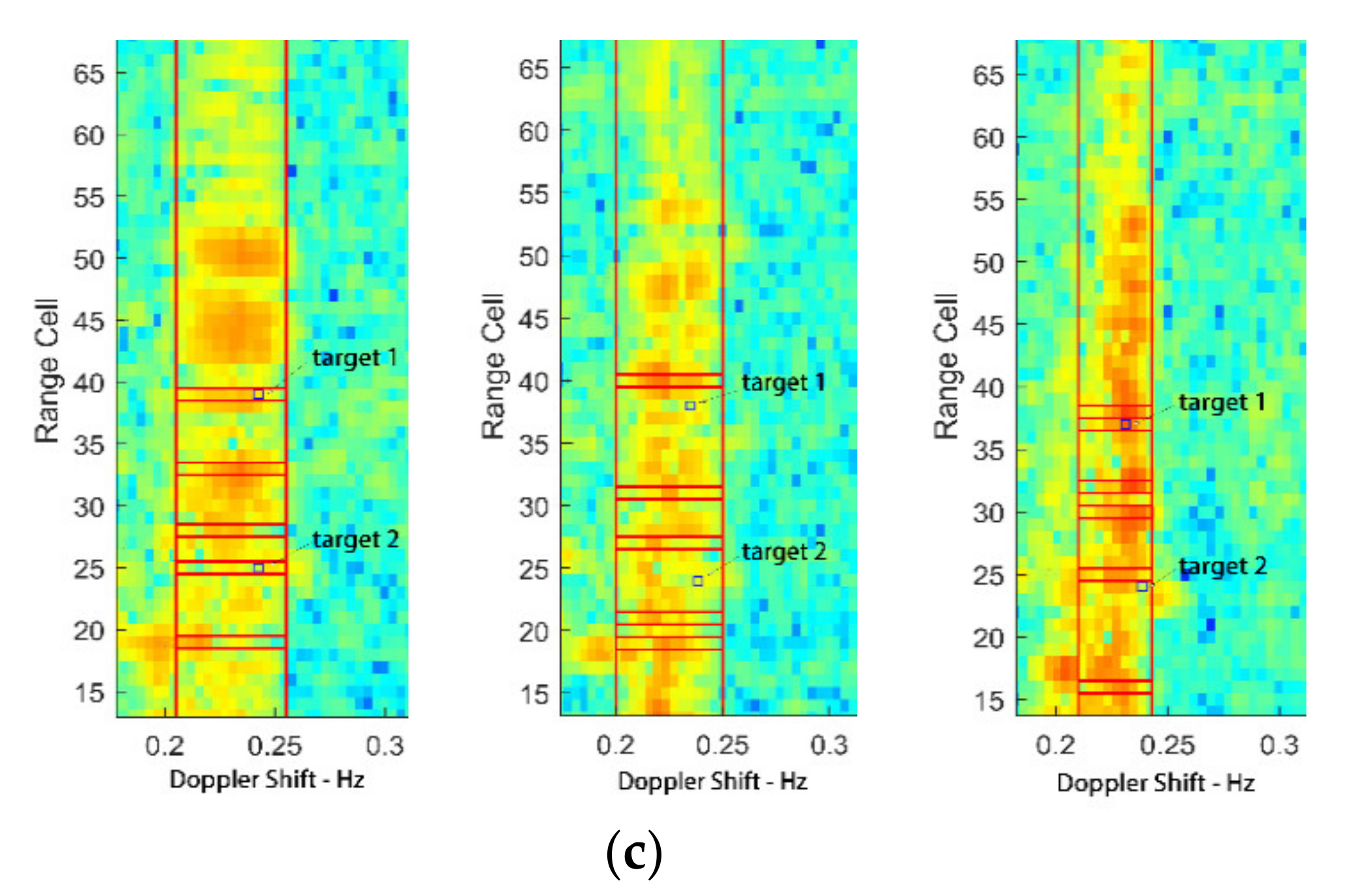
The diffusion of the target point in the HFSWR echo signal will cause the TFIs of one or two range cells above and below the target point to show similar features. If no subsequent processing is performed, the detection of Figure 10a–c will result in a high false-alarm rate. To improve detection, this paper proposes a novel scheme via the correlation of multiple frames of the RD spectrums of several range cells by accumulating the signal through a coherent accumulation time of five minutes. On the basis of the velocity range of the vessels, three batches of data are obtained every five minutes for correlation detection. The target point in the radar echo signal will appear diffuse in this situation, and the continuous data diffusion will affect detection accuracy, so if a certain range cell appears to be the target, then the adjacent distance unit will also appear to have similar characteristics and thus be detected as a target. In the correlation process, a false alarm will appear, but the false-alarm rate will be greatly reduced.
From the above situation, three batches of interrelated field shipborne HFSWR data from a certain sea trip are taken for detection, and the single-batch detection results are shown in Figure 10a–c. It can be seen that each batch of data has a high false-alarm rate. However, after three batches are correlated to obtain the results in Figure 10d, the rate is greatly reduced and the accuracy of target detection is greatly improved.
5.2. Field Experiment
Following the above detection rules, three continuous batches of field data from the shipborne HFSWR were taken for detection. The field shipborne HFSWR experiment were conducted at Huanghai, China, with 5-antenna array radar at working frequency 4.7 MHz. The results of each batch and of the correlated three batches are shown in Figure 10. Each batch of data has a large false-alarm rate, but after three batches are correlated, the rate has been greatly reduced and the accuracy of target detection has been greatly improved.
Figure 11 compares the results of the improved CFAR method, the CNN method [18], and the proposed method. The CNN and improved CFAR methods are not ideal for detecting the submerged targets due to sea clutter diffusion and low SNR, and the proposed method is better for target detection in the sea clutter–covered area.
In the tracking detection of vessel targets 1 and 2, a batch of data were taken every five minutes for fifty minutes and transformed to obtain RD spectrum images with a total of 20 target points. The results of the detection of RD spectra by three methods were evaluated by detection rate , false-alarm rate , and missed-alarm rate , in Table 6 The equations for calculating the three indicators are as follows:
where TP is the detected real target points, FN is the undetected target points, TP + FN is the total number of target points, and FP is the detected false target points.
From Table 6, it can be seen that the improved CFAR method is less effective in low SNR conditions, and the accuracy of CNN has improved over that of the improved CFAR, but the false-alarm rate is still significantly higher than that of the proposed method. The proposed method performs better than the other two methods in having a lower false-alarm rate and a higher detection rate.
6. Conclusions
In this paper, we have modeled the factors affecting the frequency of the shipborne HFSWR echo signal, including the platform’s 6-DOF motion, forward motion, and sea currents, and we obtained the width of the sea clutter spread in the radar echoes under the influence of these factors. The accuracy of the model in predicting the sea clutter spreading area was verified by both simulation and the in situ measured shipborne HFSWR data. The TF analysis method SET was applied to obtain the TFI of the area covered by the sea clutter, which showed different TF characteristics, to determine whether the area contained target points. On the basis of the sea clutter identification results, the target locations were classified by CNN to judge whether the clutter region contained targets. Finally, the location of the target was determined by correlating multiple frames of RD spectra. The proposed method was verified to be effective in detecting targets in regions covered by sea clutter through field shipborne HFSWR experimental data, which showed that the method performed better than the conventional detection methods, having a higher detection rate and a lower false-alarm rate.
Author Contributions
Conceptualization: L.Z.; methodology: T.W. and G.L.; software: T.W.; validation: T.W. and L.Z.; writing—original draft preparation: L.Z. and T.W.; writing—review and editing: G.L., T.W. and L.Z. are co-first authors and contribute equally to this work. All authors have read and agreed to the published version of the manuscript.
Funding
This project is sponsored by the National Natural Science Foundation of China (No. 51979256).
Conflicts of Interest
The authors declare no conflict of interest. The funders had no role in the design of the study; the collection, analyses, or interpretation of data; the writing of the manuscript; or the decision to publish the results.
References
- Zhang, L.; Mao, D.; Niu, J.; Wu, Q.M.J.; Ji, Y. Continuous Tracking of Targets for Stereoscopic HFSWR Based on IMM Filtering Combined with ELM. Remote Sens. 2020, 12, 272. [Google Scholar] [CrossRef]
- Xie, J.; Yuan, Y.; Liu, Y. Experimental analysis of sea clutter in shipborne HFSWR. IEE Proc. Radar Sonar Navig. 2001, 148, 67–71. [Google Scholar] [CrossRef]
- Walsh, J.; Huang, W.; Gill, E. The First-Order High Frequency Radar Ocean Surface Cross Section for an Antenna on a Floating Platform. IEEE Trans. Antennas Propag. 2010, 58, 2994–3003. [Google Scholar] [CrossRef]
- Walsh, J.; Huang, W.; Gill, E. The second-order high frequency radar ocean surface cross section for an antenna on a floating platform. IEEE Trans. Antennas Propag. 2012, 60, 4804–4813. [Google Scholar] [CrossRef]
- Ma, Y.; Gill, E.W.; Huang, W. High Frequency Radar Cross Sections of the Ocean Surface Incorporating Pitch and Roll Motions of a Floating Platform. In Proceedings of the 2018 OCEANS-MTS/IEEE Kobe Techno-Oceans (OTO), Kobe, Japan, 28–31 May 2018; pp. 1–4. [Google Scholar]
- Yao, G.; Xie, J.; Huang, W. First-order ocean surface cross-section for shipborne HFSWR incorporating a horizontal oscillation motion model. IET Radar Sonar Navig. 2018, 12, 973–978. [Google Scholar] [CrossRef]
- Gill, E.W.; Ma, Y.; Huang, W. Motion compensation for high-frequency surface wave radar on a floating platform. IET Radar Sonar Navig. 2018, 12, 37–45. [Google Scholar] [CrossRef]
- Zhang, X.; Yang, Q.; Sun, J.; Deng, W. A Space-Time Model of Sea Echo with Shipborne HFSWR Platform Under Varying Velocity Motion. In Proceedings of the 2018 International Symposium on Antennas and Propagation (ISAP), Busan, Korea, 23–26 October 2018; pp. 1–2. [Google Scholar]
- Yang, K.; Zhang, L.; Niu, J.; Ji, Y.; Wu, Q.M.J. Analysis and Estimation of Shipborne HFSWR Target Parameters Under the Influence of Platform Motion. IEEE Trans. Geosci. Remote Sens. 2021, 59, 4703–4716. [Google Scholar] [CrossRef]
- Xiao, Z.; Yan, Z. Radar Emitter Identification Based on Novel Time-Frequency Spectrum and Convolutional Neural Network. IEEE Commun. Lett. 2021, 25, 2634–2638. [Google Scholar] [CrossRef]
- Huang, Z.-L.; Zhang, J.; Zhao, T.-H.; Sun, Y. Synchrosqueezing S-Transform and Its Application in Seismic Spectral Decomposition. IEEE Trans. Geosci. Remote Sens. 2016, 54, 817–825. [Google Scholar] [CrossRef]
- Yu, G.; Wang, Z.; Zhao, P. Multisynchrosqueezing Transform. IEEE Trans. Ind. Electron. 2019, 66, 5441–5455. [Google Scholar] [CrossRef]
- Yu, G.; Yu, M.; Xu, C. Synchroextracting Transform. IEEE Trans. Ind. Electron. 2017, 64, 8042–8054. [Google Scholar] [CrossRef]
- Cai, J.; Zhou, H.; Huang, W.; Wen, B. Ship Detection and Direction Finding Based on Time-Frequency Analysis for Compact HF Radar. IEEE Geosci. Remote Sens. Lett. 2021, 18, 72–76. [Google Scholar] [CrossRef]
- Li, Q.; Zhang, W.; Li, M.; Niu, J.; Jonathan Wu, Q.M. Automatic Detection of Ship Targets Based on Wavelet Transform for HF Surface Wavelet Radar. IEEE Geosci. Remote Sens. Lett. 2017, 14, 714–718. [Google Scholar] [CrossRef]
- Chen, Z.; He, C.; Zhao, H.; Xie, F. Enhanced multi-target detection for HFSWR by sparse-recovery-based 2-D MUSIC. In Proceedings of the OCEANS 2017-Anchorage, Anchorage, AK, USA, 18–21 September 2017; pp. 1–5. [Google Scholar]
- Wang, Y.; Mao, X.; Zhang, J.; Ji, Y. Detection of Vessel Targets in Sea Clutter Using In Situ Sea State Measurements With HFSWR. IEEE Geosci. Remote Sens. Lett. 2018, 15, 302–306. [Google Scholar] [CrossRef]
- Wu, M.; Zhang, L.; Niu, J.; Wu, Q.M.J. Target Detection in Clutter/Interference Regions Based on Deep Feature Fusion for HFSWR. IEEE J. Sel. Top. Appl. Earth Obs. Remote Sens. 2021, 14, 5581–5595. [Google Scholar] [CrossRef]
- Chang, G.; Li, M.; Xie, J.; Zhang, L.; Yu, C.; Ji, Y. Ocean Surface Current Measurement Using Shipborne HF Radar: Model and Analysis. IEEE J. Ocean. Eng. 2016, 41, 970–981. [Google Scholar] [CrossRef]
- Chang, G.; Li, M.; Zhang, L.; Ji, Y.; Xie, J. Measurements of ocean surface currents using shipborne High-Frequency radar. In Proceedings of the IEEE Radar Conference, Cincinnati, OH, USA, 19–23 May 2014. [Google Scholar] [CrossRef]
- Szegedy, C.; Liu, W.; Jia, Y.; Sermanet, P.; Reed, S.; Anguelov, D.; Erhan, D.; Vanhoucke, V.; Rabinovich, A. Going deeper with convolutions. In Proceedings of the 2015 IEEE Conference on Computer Vision and Pattern Recognition (CVPR), Boston, MA, USA, 7–12 June 2015; pp. 1–9. [Google Scholar] [CrossRef]
- Krizhevsky, A.; Sutskever, I.; Hinton, G.E. ImageNet classification with deep convolutional neural networks. Commun. ACM 2017, 60, 84–90. [Google Scholar] [CrossRef]
- Simonyan, K.; Zisserman, A. Very Deep Convolutional Networks for Large-Scale Image Recognition. Comput. Sci. 2014, preprint. [Google Scholar] [CrossRef]
Figure 1.
RD spectra of HFSWR. (a) RD spectra of shore−based HFSWR. (b) RD spectra of shipborne HFSWR.
Figure 1.
RD spectra of HFSWR. (a) RD spectra of shore−based HFSWR. (b) RD spectra of shipborne HFSWR.

Figure 2.
Detection framework for targets concealed in clutter regions with shipborne HFSWR.

Figure 3.
Schematic diagram of the platform’s 6-DOF motion.

Figure 4.
Schematic diagram of forward movement and motion due to ocean currents.

Figure 5.
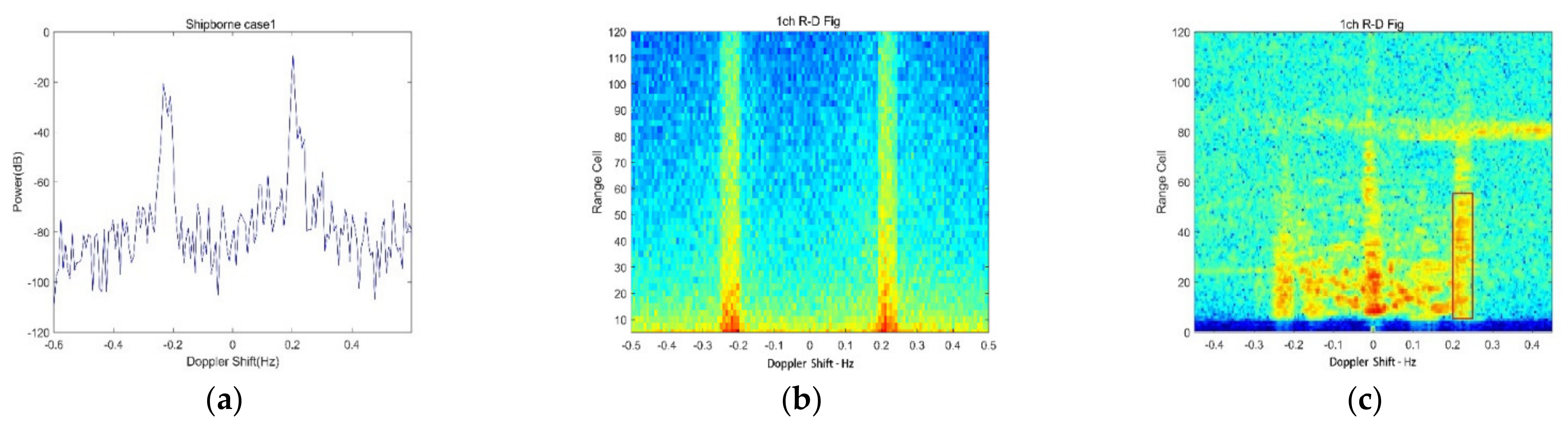
Simulation and measured results. (a) Frequency-domain result of simulated sea clutter. (b) Simulation of RD spectrum. (c) Measured RD spectrum results.
Figure 5.
Simulation and measured results. (a) Frequency-domain result of simulated sea clutter. (b) Simulation of RD spectrum. (c) Measured RD spectrum results.

Figure 6.
TF image. (a) STFT TF image. (b) SET TF image.

Figure 7.
(a) SET of targets with sea clutter. (b) SET of pure sea clutter.

Figure 8.
Schematic diagram of transmitting and receiving antenna positions.

Figure 9.
(a) TFI of sea clutter. (b) TFI of targets with sea clutter.

Figure 10.
(a–c) Single−batch test results. (d) Final test result after correlation.

Figure 11.
(a) Proposed method test result. (b) CNN test result. (c) Improved CFAR test result.


Table 1.
6-DOF, forward movement and current simulation parameters.
| Parameter Name | Numerical Values | Unit |
|---|---|---|
| Roll angle | 0.2410 | rad |
| Pitch angle | 1.1807 | rad |
| Declination angle | 49.2000 | rad |
| Sway speed | 0.2000 | m/s |
| Surge speed | 0.2000 | m/s |
| Roll speed | 0.1000 | m/s |
| Pitch speed | 0.0900 | m/s |
| Yaw Speed | 0.1700 | m/s |
| Forward movement speed | 0.2000 | m/s |
| Current speed | 0.3448 | m/s |
Table 2.
Results of sea-wave spreading.
| Pattern | Width (Hz) |
|---|---|
| Theoretical Calculations | 0.050 |
| Simulation Result | 0.050 |
| Measured Result | 0.048 |
Table 3.
Shipborne HFSWR Parameters.
| Parameters | Values |
|---|---|
| Transmit signal | FMICW |
| Operating frequency (MHz) | 4.7 |
| Coherent integration time (s) | 300 |
| Number of antennas | 5 |
| Antenna spacing | Non-uniform array |
Table 4.
GoogLeNet network structure.
| Type | Patch Size/Stride | Output Size | Depth | #1 × 1 | #3 × 3 Reduce | #3 × 3 | #5 × 5 Reduce | #5 × 5 | Pool Proj | Params | Ops |
|---|---|---|---|---|---|---|---|---|---|---|---|
| convolution | 7 × 7/2 | 112 × 112 × 64 | 1 | 2.7 K | 34 M | ||||||
| max pool | 3 × 3/2 | 56 × 56 × 64 | 0 | ||||||||
| convolution | 3 × 3/1 | 56 × 56 × 192 | 2 | 64 | 192 | 112 K | 360 M | ||||
| max pool | 3 × 3/2 | 28 × 28 × 192 | 0 | ||||||||
| Inception(3a) | 28 × 28 × 256 | 2 | 64 | 96 | 128 | 16 | 32 | 32 | 159 K | 128 M | |
| Inception(3b) | 28 × 28 × 480 | 2 | 128 | 128 | 192 | 32 | 96 | 64 | 380 K | 304 M | |
| Max pool | 3 × 3/2 | 14 × 14 × 480 | 0 | ||||||||
| Inception(4a) | 14 × 14 × 512 | 2 | 192 | 96 | 208 | 16 | 48 | 64 | 364 K | 73 M | |
| Inception(4b) | 14 × 14 × 512 | 2 | 160 | 112 | 224 | 24 | 64 | 64 | 437 K | 88 M | |
| Inception(4c) | 14 × 14 × 512 | 2 | 128 | 128 | 256 | 24 | 64 | 64 | 463 K | 100 M | |
| Inception(4d) | 14 × 14 × 528 | 2 | 112 | 144 | 288 | 32 | 64 | 64 | 580 K | 119 M | |
| Inception(4e) | 14 × 14 × 832 | 2 | 256 | 160 | 320 | 32 | 128 | 128 | 840 K | 170 M | |
| Max pool | 3 × 3/2 | 7 × 7 × 832 | 0 | ||||||||
| Inception(5a) | 7 × 7 × 832 | 2 | 256 | 160 | 320 | 32 | 128 | 128 | 1072 K | 54 M | |
| Inception(5b) | 7 × 7 × 1024 | 2 | 384 | 192 | 384 | 48 | 128 | 128 | 1388 K | 71 M | |
| Avg pool | 7 × 7/1 | 1 × 1 × 1024 | 0 | ||||||||
| Dropout(30%) | 1 × 1 × 1024 | 0 | |||||||||
| Linear | 1 × 1 × 1000 | 1 | 1000 K | 1 M | |||||||
| Softmax | 1 × 1 × 1000 | 0 |
Table 5.
Detection results of the classification methods.
| Network Structure | GoogLeNet | AlexNet | VGG-16 |
|---|---|---|---|
| Total number of tests | 26 | 26 | 26 |
| Detected correctly | 22 | 20 | 21 |
| Time | 1.269 | 0.6 | 2.8 |
| Accuracy | 84.6% | 76.9% | 80.77% |
Table 6.
Comparison of the three methods with several indexes over ten RD spectra in half an hour.
| Method | Our Method | CNN | Improved CFAR |
|---|---|---|---|
| Target total number of tests | 20 | 20 | 20 |
| Detected correctly | 18 | 13 | 16 |
| 10% | 53.57% | 54.55% | |
| 10% | 35% | 25% | |
| 90% | 65% | 75% |
Publisher’s Note: MDPI stays neutral with regard to jurisdictional claims in published maps and institutional affiliations. |
© 2022 by the authors. Licensee MDPI, Basel, Switzerland. This article is an open access article distributed under the terms and conditions of the Creative Commons Attribution (CC BY) license (https://creativecommons.org/licenses/by/4.0/).
Share and Cite
MDPI and ACS Style
Wang, T.; Zhang, L.; Li, G. Shipborne HFSWR Target Detection in Clutter Regions Based on Multi-Frame TFI Correlation. Remote Sens. 2022, 14, 4192. https://doi.org/10.3390/rs14174192
AMA Style
Wang T, Zhang L, Li G. Shipborne HFSWR Target Detection in Clutter Regions Based on Multi-Frame TFI Correlation. Remote Sensing. 2022; 14(17):4192. https://doi.org/10.3390/rs14174192
Chicago/Turabian StyleWang, Tao, Ling Zhang, and Gangsheng Li. 2022. "Shipborne HFSWR Target Detection in Clutter Regions Based on Multi-Frame TFI Correlation" Remote Sensing 14, no. 17: 4192. https://doi.org/10.3390/rs14174192
Note that from the first issue of 2016, this journal uses article numbers instead of page numbers. See further details here.